NCrystal : a library for thermal neutron transport

Abstract

An open source software package for modelling thermal neutron transport is presented. The code facilitates Monte Carlo-based transport simulations and focuses in the initial release on interactions in both mosaic single crystals as well as polycrystalline materials and powders. Both coherent elastic (Bragg diffraction) and incoherent or inelastic (phonon) scattering are modelled, using basic parameters of the crystal unit cell as input.

Included is a data library of validated crystal definitions, standalone tools and interfaces for C++, C and Python programming languages. Interfaces for two popular simulation packages, Geant4 and McStas, are provided, enabling highly realistic simulations of typical components at neutron scattering instruments, including beam filters, monochromators, analysers, samples, and detectors. All interfaces are presented in detail, along with the end-user configuration procedure which is deliberately kept user-friendly and consistent across all interfaces.

An overview of the relevant neutron scattering theory is provided, and the physics modelling capabilities of the software are discussed. Particular attention is given here to the ability to load crystal structures and form factors from various sources of input, and the results are benchmarked and validated against experimental data and existing crystallographic software. Good agreements are observed.

PROGRAM SUMMARY

Manuscript Title: NCrystal : a library for thermal neutron transport
Authors: X.-X. Cai and T. Kittelmann
Program Title: NCrystal
Journal Reference:
Catalogue identifier:
Licensing provisions: Apache License, Version 2.0 (for core NCrystal).
Programming language: C++, C and Python
Operating system: Linux, OSX, Windows
Keywords:
Thermal neutron scattering, Simulations, Monte Carlo, Crystals, Bragg diffraction
Classification: 4, 7.6, 8, 17
External routines/libraries: Geant4, McStas
Nature of problem:
Thermal neutron transport in structured materials is inadequately supported in popular Monte Carlo transport applications, preventing simulations of a range of otherwise interesting setups.
Solution method:
Provide models for thermal neutron transport in flexible open source library, to be used standalone or as backend in existing Monte Carlo packages. Facilitate validation and work sharing by making it possible to share material configurations between supported applications.

1 Introduction

The modelling of neutron transport through matter dates back to the efforts aimed at tackling neutron diffusion problems in the middle of the twentieth century, closely tied to the introduction of general purpose computers and the inception of the method of Monte Carlo simulations [1]. Since then, the needs for transport simulations involving neutrons have expanded, with a wide range of applications in radiation protection, reactor physics, radiotherapy, and scattering instruments at spallation or reactor sources. To facilitate such simulations a plethora of Monte Carlo simulation applications exists today, which for the purposes here can be divided into two categories: general purpose applications [2, 3, 4, 5, 6, 7, 8, 9, 10, 11], capable of modelling a variety of particle types in flexible geometrical layouts, and specialised applications [12, 13, 14, 15, 16, 17] dealing with the design of neutron scattering instruments. Applications in the latter group is focused on aspects of individual scatterings of thermal neutrons, but generally lack capabilities for dealing with arbitrarily complex geometries and the inclusion of physics of particles other than thermalised neutrons.

On the other hand, the general purpose Monte Carlo applications are typically oriented towards use-cases in fields such as reactor physics, high energy physics, and radiation protection, and as a rule neglect all material structure and effects of inter-atomic bindings – resorting instead to the approximation of treating all materials as a free gas of unbound atoms with no mutual interactions. This approximation is suitable at higher incident energies, but for neutrons it breaks down at the thermal scale where their wavelengths and kinetic energies are comparable to the typical distances and excitational energies resulting from inter-atomic bindings. The only presently available option for improved modelling of thermal neutron interactions involves the utilisation of specially prepared data files of differential cross section data. These “scattering kernels” are only readily available in neutron evaluation libraries, e.g. [18], for the dozen or so materials which have traditionally played an important role for shielding or moderation purposes at nuclear facilities. For other materials, scattering kernels must be carefully crafted using non-trivial procedures (like the application of delicate and computationally expensive molecular dynamics models [19]) and in practice this is rarely done. Furthermore, some aspects of thermal neutron scatterings are in practice ignored when modelling is exclusively based on scattering kernels: since nuclear reactor physics has historically mostly been focused on inelastic and multiple-scattering phenomena, it is usually not possible to include a precise model of the a priory highly significant process of Bragg diffraction into the setup for crystalline materials. At thermal energies, Bragg diffraction is the dominant process for many relevant materials, and although it is an elastic scattering process which does not change the neutron energy, it sends neutrons to characteristic solid angles and can therefore critically influence the geometrical reach of neutrons through a given geometry.

It is thus not currently straight-forward to carry out simulations which at the same time incorporate consistent and realistic physics models for neutrons at both high and low energy scales in general materials, while simultaneously supporting flexible geometrical layouts and the treatment of particles other than neutrons. Such simulations would nonetheless be remarkably useful, in particular when considering aspects of neutron scattering instruments [20, 21]. Here, precise modelling of individual neutron scatterings is crucial in all beam-line components, while detailed understanding of background levels, the effects of shielding, or the workings of neutron detectors, require incorporation of detailed geometrical layouts and additional physics such as modelling of gammas, fast neutrons, and energy depositions resulting from secondary particles released upon neutron capture. Other examples include the design of advanced moderators or reflectors for novel reactors or neutron spallation sources, and proton or neutron-based radiotherapy, in which adverse irradiation from neutrons are abundant and an increasing concern [22, 23].

The NCrystal toolkit presented here is aimed at remedying the situation. Rather than introducing an entirely new application, it is designed as a flexible backend, able to plug the gaps where existing Monte Carlo applications are lacking in capabilities for treating thermal neutrons in structured materials. It was originally developed to facilitate the design and optimisation of neutron detectors for the European Spallation Source, presently under construction in Lund, Sweden [24, 25, 26, 27, 20], but is intended to be as widely useful as possible – not only as a service to the community, but also to ultimately ensure a higher level of quality for the toolkit itself due to feedback and validation from a larger potential userbase. Although dedicated utilities for calculating various properties of thermal neutrons exists [28, 29, 30, 31], the scope of NCrystal is different, delivering at the same time an ambitious set of physics models, a flexible object oriented design, multiple interfaces and bindings, an open approach to development, and not the least a user-friendly method of configuration. The core functionality is implemented as an open source and highly portable C++ library with no third-party dependencies, and comes with language bindings for all versions of C++, C or Python in widespread usage today. The current code is released with version number 1.0.0 and under a highly liberal open source license [32]. Included in the release is additionally tools, examples, data files, and a configuration file for CMake [33] with which everything can be built and installed. A website [34] has been set up for the NCrystal project, on which users will be able to interact with developers, locate future updates, and access relevant documentation.

Concerning NCrystal’s capabilities for physics simulations, the work has so far focused on facilitating realistic simulations of both inelastic and elastic physics of thermal neutrons as they scatter in certain common bulk crystalline materials. Namely those which can be described in terms of a statistical arrangements of microscopic perfect crystals, and for which the neutron’s interaction probabilities are not so strong as to break down the Born approximation. Additionally, material configuration can be carried out based simply on a brief description of the crystal structures. All together, the framework thus provides realistic thermal neutron physics in a large range of powdered, polycrystalline or mosaic single crystals readily used at neutron scattering facilities in beam filters, monochromators, analysers, samples, detectors, and shielding. What is currently not supported, given the mentioned constraints, is surface effects, materials that are either non-crystalline or textured, and effects related to a break-down of the Born approximation including the strong reflections found in neutron guide systems, or the strong diffraction effects encountered in certain macroscopic crystal systems such as synthetically grown Silicon. Future developments might address some of those deficiencies, depending on community interest and resources.

The present paper will present the NCrystal framework itself, including interfaces, configuration, and data input options. Although a brief overview of physics capabilities will be provided, detailed discussions of the implementation of actual thermal neutron scattering models are beyond the scope of the present paper, and will be the subject of dedicated publications at a later date. After a review of the relevant theoretical concepts in Section 2, the design and implementation of the core NCrystal code is presented in Section 3. Section 4 presents the capabilities for initialising relevant parameters of modelled crystals from various data sources, introduces the library of data files included with NCrystal and discusses how the loaded results have been validated. Section 5 presents the uniform method for material configuration intended for most end-users, and an overview of the existing language bindings and application interfaces is provided in Section 6. Finally, a discussion of future directions and planned improvements is carried out in Section 7.

2 Theoretical background

Rather than intending to be an exhaustive treatment, this section will provide a brief overview of crystals and neutron scattering, introducing relevant concepts, models and terminology needed for the purposes of the present discussions of NCrystal. Naturally, relevant references to more extensive background literature are provided for readers seeking more information.

2.1 Crystals

Although support for other types of materials is likely to be added eventually, the present scope of NCrystal is restricted to crystals. Consequently, a few basic concepts will be introduced in the following. Further details can be found in [35, 36, 37, 38].

Informally, a crystal can be described as an arrangement of bound atoms which is built up by the periodic repetition of a basic element in all three spatial directions. This repeated element is known as the unit cell and is typically chosen such that it is the smallest such cell that reflects the symmetry of the structure. In an idealised setting, the crystal structure would be infinite, but in practice it is sufficient that the unit cell is much smaller than the entire structure. The choice of unit cell for a given crystal is not always unique, but it is always possible to select one which is a parallelepiped spanned by three linearly independent basis vectors $\vec{a}$, $\vec{b}$ and $\vec{c}$. By convention they are defined by their respective lengths, $a$, $b$, and $c$, and the angles between them: $\alpha\equiv\angle(\vec{b},\vec{c})$, $\beta\equiv\angle(\vec{a},\vec{c})$, and $\gamma\equiv\angle(\vec{a},\vec{b})$. The crystal structure is completed by the additional specification of the contents of the unit cell, often provided in coordinates $(x,y,z)$ relative to the crystal axes. The position of the $i$th constituent in the unit cell is thus given by:

$$\vec{p}_{i}=x_{i}\vec{a}+y_{i}\vec{b}+z_{i}\vec{c},\qquad x_{i},y_{i},z_{i}\in[0,1)$$ (1)

Crystals exhibit a discrete symmetry under spatial translation with the vectors:

$$\vec{R}_{mno}=m\vec{a}+n\vec{b}+o\vec{c},\qquad m,n,o\in\mathbb{Z}$$ (2)

Apart from a trivial global offset, coordinates of all constituents in the entire crystal are given by $\vec{R}_{mno}+\vec{p}_{i}$ for all combinations of $mno$ and $i$. The translational symmetry means that any function representing features of the crystal system (such as particle densities) will obey:

$$f(\vec{r})=f(\vec{r}+\vec{R}_{mno})$$ (3)

Additional symmetries under rotations, reflections or inversions are possible, depending on the detailed shape and contents of the unit cell. The symmetry properties of a crystal are described by the concept of space groups, and it is possible to describe any spatial crystal symmetry by one of only 230 such groups. These groups can be divided into 7 general classes of crystal systems. Loosely ordered from lowest to highest symmetry they are: triclinic, monoclinic, orthorhombic, tetragonal, trigonal, hexagonal, and cubic. The space groups are defined and described exhaustively in [38].

The space group of a given crystal structure naturally depends on the unit cell positions of constituents, $\vec{p}_{1},\ldots,\vec{p}_{N}$. Conversely, it is possible to construct the full list of these positions by applying the symmetry operators of a given space group to a smaller number of so-called Wyckoff positions [39]. It is indeed very common to find crystal structures defined solely in terms of their space group, unit cell shape and dimensions, and a list of elements and associated Wyckoff positions.

The set of points at positions $\vec{R}_{mno}$ for all integers $m$, $n$, and $o$, constitutes the crystal lattice. In each such lattice, there exist an infinite number of families of evenly spaced parallel planes passing through the lattice points. Each such family of lattice planes is described by a common plane normal $\hat{n}$ and an interplanar distance $d$ (also known as the $d$-spacing), with planes passing through the points $jd\hat{n}$ for all $j\in\mathbb{Z}$. Particle diffraction in a crystal occurs in the form of reflections from such families of lattice planes. The task of finding and classifying these families is often done in the so-called reciprocal lattice in momentum-space, which is the Fourier transform of the direct lattice. The basis vectors of the reciprocal lattice are given by:

$$\vec{\tau}_{a}=\frac{2\pi}{V_{\text{uc}}}\left(\vec{b}\times\vec{c}\right),\quad\vec{\tau}_{b}=\frac{2\pi}{V_{\text{uc}}}\left(\vec{c}\times\vec{a}\right),\quad\vec{\tau}_{c}=\frac{2\pi}{V_{\text{uc}}}\left(\vec{a}\times\vec{b}\right)$$ (4)

Where $V_{\text{uc}}=\vec{a}\cdot(\vec{b}\times\vec{c})$ is the unit cell volume. The points in the reciprocal lattice are thus given by:

$$\vec{\tau}_{hkl}=h\vec{\tau}_{a}+k\vec{\tau}_{b}+l\vec{\tau}_{c},\qquad h,k,l\in\mathbb{Z}$$ (5)

As will be motivated in Section 2.3, it can be shown that each point in the reciprocal lattice corresponds to a family of equidistant lattice planes in the direct lattice. The family of planes corresponding to $\vec{\tau}_{hkl}$ will be indexed by the $hkl$ value (known as its Miller index), and has interplanar spacing $d_{hkl}=2\pi/\tau_{hkl}$ and normal $\hat{n}=\hat{\tau}_{hkl}=\vec{\tau}_{hkl}/\tau_{hkl}$.

In most real systems, regions in which the crystal lattice is continuous and the defining translational invariance of Eq. 3 is unbroken, exists only at the microscopic scale. Macroscopic crystals are then built up from these independently oriented grains of perfect crystals (also known as “crystallites”), and the actual distribution of orientations will not only be related to various macroscopic material properties, but will influence interaction probabilities when the system is probed with impinging particles. As long as the grain sizes are small compared to the regions of material being probed, these effects can be accounted for in a statistical manner – for instance by integrating microscopic interaction cross sections over the distribution of crystallite orientations in order to arrive at effective macroscopic cross sections. Such integrations are particularly trivial to perform in the extreme case where the orientation of individual crystallites are completely independent and uniformly distributed over all solid angles. This model, known as the powder approximation, is not only suitable for modelling actual powdered crystalline samples, but can also be used to approximate interactions in polycrystalline materials like metals or ceramics – especially when the level of correlation in crystallite orientation (“texture”) is low or when the setup involves sufficiently large geometries or spread in incoming particles that effects due to local correlations are washed out. An example of this would be the case where polycrystalline metal support structures are placed in various places throughout a neutron instrument. On the other hand, interactions in a highly textured polycrystalline sample placed in a tightly focused beam of probe particles might not be very well described by the powder approximation.

In another extreme, all crystallites are almost co-aligned in so-called mosaic crystals, with the exact distribution around the common axis of alignment given by the mosaicity distribution. In the simple isotropic case, this distribution is a Gaussian function of the angular displacement, with the corresponding width (referred to as the mosaicity of the crystal) having typical values anywhere from a few arc seconds to a few degrees. In NCrystal, such Gaussian mosaic crystals are referred to as “single crystals”, due to the large degree of crystallite alignment throughout the material.

Some materials are better described by other mosaicity distributions, including anisotropic ones where the distribution is not symmetric with respect to all axes. A particular anisotropic distribution supported by NCrystal is one in which crystallites are aligned around one particular axis, but appearing with random rotations around the same axis. Such distributions occur in stratified or layered crystals, like pyrolytic graphite, in which certain planes of atoms tend to have strongly aligned normals in all crystallites, but no strong alignment for the rotation of the same planes around their normals.

2.2 Scattering theory

The theory of thermal neutron scatterings in condensed matter is thoroughly treated in the literature, see for instance [40, 41, 42]. The discussion in the present and following sections is to a large degree inspired by [40, 41].

Scattering in materials by thermal neutrons, taken here to loosely mean energies below or at the $\text{\,}\mathrm{eV}\text{/}$ scale or wavelengths above or at the $\text{\,}\mathrm{nm}\text{/}$ scale, can be described via point-like neutron-nuclei interactions or magnetic dipole interactions between the neutron and any unpaired electrons in the target material. For unpolarised neutrons and samples, the latter can be largely ignored [43] and the current discussion will not concern itself with such magnetic interactions, nor are they currently modelled in NCrystal – although there is nothing fundamental preventing their inclusion in the future.

Thermal neutrons carry such low energy that in practice no emission of secondary particles occurs during pure scattering interactions. As a consequence, scattering of unpolarised neutrons can be completely described in terms of the differential cross section for scattering the incident neutron with wavevector $\vec{k}_{i}$ into the wavevector $\vec{k}_{f}$. Based on the Born approximation or Fermi’s golden rule, this differential cross section is related to quantum mechanical transition amplitudes by the so-called master equation for thermal neutron scattering:

$$\frac{d^{2}\sigma_{\vec{k}_{i}\Rightarrow\vec{k}_{f}}}{d\Omega_{f}dE_{f}}=\frac{k_{f}}{k_{i}}\frac{(2\pi)^{4}m^{2}}{\hbar^{4}}\sum_{\eta_{i},\eta_{f}}{p(\eta_{i})|\langle\eta_{f},\vec{k}_{f}|\boldsymbol{V}|\eta_{i},\vec{k}_{i}\rangle|^{2}\delta(\hbar\omega+{\Delta}E_{\eta})}$$ (6)

Here $m$ is the neutron mass, indices $i$ and $f$ denotes initial and final states respectively, ${\eta_{j}}$ represents a complete set of eigenstates of the target system, $p(\eta_{i})$ represents the initial occupation levels of target states, and $\boldsymbol{V}$ is the interaction potential. Furthermore, $\hbar\omega=E_{f}-E_{i}$ and ${\Delta}E_{\eta}\equiv E_{\eta_{f}}-E_{\eta_{i}}$ represents the total energy change of the neutron and target system respectively. At this point it might be useful to recall that in addition to wavenumber, $k=|\vec{k}|$, the energy state of a non-relativistic neutron might equally be characterised in terms of energy $E$, momentum $p$, velocity $v$, or wavelength $\lambda$, related by $p={\hbar}k$, $2E=mv^{2}=p^{2}/m$, and $\lambda=2\pi/k$.

Before continuing with the evaluation of Eq. 6, it is important to understand its validity and applicability. Based on the Born approximation, the perturbation experienced by the initial neutron wave function during the scattering is assumed to be small, so it is possible to neglect secondary scattering of waves created as a result of the primary scattering. The sum in Eq. 6 implies that the resulting cross sections will grow with the size of the target system, and therefore the validity of the equation will eventually break down as the size of the target system grows and the probability for secondary scattering becomes non-negligible. In reality this issue is circumvented in the context of Monte Carlo transport simulations in which neutron transport is modelled in a series of steps between independent scatterings, with each simulated step length depending on the actual mean free path length predicted by the cross section in Eq. 6. High cross sections will automatically lead to small step lengths, and therefore only a small part of the sample will be traversed for each application of Eq. 6. Simulations employing such stepping will therefore to some degree account for multiple scattering phenomena like extinction effects in crystal diffraction. This effective subdivision of a target system into smaller decoherent systems is, however, only possible if the linear scale over which any symmetries in the material structure exists is small compared to the mean free path lengths involved, so wavefunctions originating from scattering in separate subsystems will be mutually incoherent. As described in Section 2.1 most real macroscopic crystals consists of independently aligned microscopic crystal grains, and in practice this ensures the necessary decoherence between different parts of the macroscopic system. The exception is the case of perfect macroscopic crystals (or mosaic crystals with vanishing mosaic spread) like some synthetic silicon crystals. For an excellent and detailed discussion about these issues, refer to [41, Sec. 11.5].

In order to proceed with the evaluation of Eq. 6, one must provide suitable representations of both interaction potential $\boldsymbol{V}$ and distributions of target states, $p(\eta_{i})$. When dealing with thermal neutrons and their relatively long wavelength, the short-range neutron-nuclei interactions can effectively be described as being point-like. An effective potential which describes them as such was introduced by Fermi [44]. For a collection of $N$ nuclei located at positions $\vec{R}_{j}$ it looks like:

$$V(\vec{r})=\frac{2\pi\hbar^{2}}{m}\sum^{N}_{j=1}b_{j}\delta(\vec{r}-\vec{R}_{j})$$ (7)

Here $b_{j}$ is the scattering length of the $j$th nucleus, an effective parameter capturing the details of the neutron-nucleus interaction which must be determined through measurements. The term scattering length stems from the fact that the corresponding cross section for scattering from a single fixed nucleus is $4{\pi}b^{2}$, equal to the classical cross section of a hard sphere of radius $2|b|$. In the presence of nuclear resonances, the scattering length becomes strongly dependent on the neutron energy. However, at the energy scale of thermal neutrons, resonances only exist for a few rare isotopes – and even then mostly at the high end of the thermal scale [45]. For the present purposes, the scattering length thus attain constant values, specific to each type of nuclei. It is additionally possible to use non-zero imaginary components of scattering lengths to represent absorption physics, however in many contexts – including the present – the two types of interactions are dealt with separately and the scattering lengths will therefore be treated as real and constant numbers. Such separation between scattering and absorption processes is valid at the $\mathcal{O}(${10}^{-4}$)$ level for thermal neutrons [46], which is considered acceptable. In fact, as the current scope of NCrystal does not cover physics of nuclear resonances, absorption processes will be dealt with using the simple – but in most cases accurate [45] – model of absorption cross sections being inversely proportional to the neutron velocity. This $1/v$ scaling can be intuitively interpreted as having the probability of absorption by a given nucleus proportional to the time spent by the neutron near the nucleus, but also follows from more careful reasoning [46, 47, 48].

It is possible to bring Eq. 6 into a form in which the sum over final states of the target system is removed and the potential is replaced with its Fourier transform. This is particularly convenient for potentials involving $\delta$-functions like Eq. 7, as these transform into constants. The resulting form is:

$$\frac{d^{2}\sigma_{\vec{k}_{i}\Rightarrow\vec{k}_{f}}}{d\Omega_{f}dE_{f}}=\frac{k_{f}}{k_{i}}S(\vec{Q},\omega)$$ (8)

where $\vec{Q}$ is the momentum transfer, $\vec{Q}\equiv\vec{k}_{f}-\vec{k}_{i}$, and $S(\vec{Q},\omega)$ is the scattering function defined by:

$$S(\vec{Q},\omega)\equiv\frac{1}{2\pi\hbar}\sum_{j,j^{\prime}=1}^{N}{b_{j}b_{j^{\prime}}}\int_{-\infty}^{\infty}dt\langle e^{-i\vec{Q}\cdot\vec{\boldsymbol{R}}_{j^{\prime}}(0)}e^{i\vec{Q}\cdot\vec{\boldsymbol{R}}_{j}(t)}\rangle e^{-i\omega t}$$ (9)

The $\langle\dots\rangle$ notation is here used to donate operator expectation values in the target system, $\langle{f}(\boldsymbol{A})\rangle=\sum_{\eta_{i}}p(\eta_{i})\langle\eta_{i}|f(\boldsymbol{A})|\eta_{i}\rangle$, with the target state weights, $p(\eta_{i})$, usually defined by a requirement for the target system to be in thermal equilibrium. The expectation value under the integral in Eq. 9 correlates the position of the nucleus $j$ at time $t$ with the position of the nucleus $j^{\prime}$ at time $0$, and will here be abbreviated as:

$$\langle{j}^{\prime},j\rangle\equiv\langle{e}^{-i\vec{Q}\cdot\vec{\boldsymbol{R}}_{j^{\prime}}(0)}e^{i\vec{Q}\cdot\vec{\boldsymbol{R}}_{j}(t)}\rangle$$ (10)

Leading to the shorter expression for the scattering function:

$$S(\vec{Q},\omega)\equiv\frac{1}{2\pi\hbar}\sum_{j,j^{\prime}=1}^{N}{b_{j}b_{j^{\prime}}}\int_{-\infty}^{\infty}dt\langle j^{\prime},j\rangle e^{-i\omega t}$$ (11)

This definition of the scattering function contains a sum over the target system under consideration (which as discussed must be of a linear size compatible with the applied Born approximation). Most such systems of interests can be divided into a number of statistically equivalent subsystems. That this is possible for crystals is obvious, since each unit cell forms such a subsystem, but subdivisions are generally possible in almost all systems, be they liquid, polymeric or gaseous in nature. The scattering function for a subsystem can be expressed as:

$$S(\vec{Q},\omega)\equiv\frac{1}{2\pi\hbar}\sum_{j,j^{\prime}=1}^{N}{\overline{b_{j}b_{j^{\prime}}}}\int_{-\infty}^{\infty}dt\langle j^{\prime},j\rangle e^{-i\omega t}$$ (12)

where now $N$ refers to the subsystem size and might for instance represent the number of nuclei in a crystal unit cell, and $\overline{b_{j}b_{j^{\prime}}}$ represents an average performed over an ensemble of equivalent subsystems. Now, neutron-nuclei scattering has the peculiarity that the scattering lengths are isotope and spin-state dependent, whereas the positions of scatterers, the nuclei, are determined by chemical properties, depending on the nuclear charge but otherwise independent of isotope or spin state. This independence means that the ensemble average of products of scattering lengths found at positions $j$ and $j^{\prime}$ obeys:

$$\overline{b_{j}b_{j^{\prime}}}=\begin{cases}\overline{b_{j}}\cdot\overline{b_{j^{\prime}}},&\text{for}\ j\neq j^{\prime}\\ \overline{b^{2}_{j}},&\text{for}\ j=j^{\prime}\end{cases}$$ (13)

With this, Eq. 12 can be written as the sum of two distinct contributions:

$$S(\vec{Q},\omega)=\, S_{\text{coh}}(\vec{Q},\omega)+S_{\text{inc}}(\vec{Q},\omega)$$ (14)

$$S_{\text{coh}}(\vec{Q},\omega)\equiv\, \frac{1}{2\pi\hbar}\sum_{j,j^{\prime}=1}^{N}{\overline{b_{j}}\cdot\overline{b_{j^{\prime}}}}\int_{-\infty}^{\infty}dt\langle j^{\prime},j\rangle e^{-i\omega t}$$ (15)

$$S_{\text{inc}}(\vec{Q},\omega)\equiv\, \frac{1}{2\pi\hbar}\sum_{j=1}^{N}{\left(\overline{b_{j}^{2}}-\left(\overline{b_{j}}\right)^{2}\right)}\int_{-\infty}^{\infty}dt\langle j,j\rangle e^{-i\omega t}$$ (16)

The terms in the coherent scattering function $S_{\text{coh}}(\vec{Q},\omega)$ directly depend on material structure as they involve pair correlations between nuclei at all positions in the material, whereas the incoherent scattering function $S_{\text{coh}}(\vec{Q},\omega)$ solely contains self-correlations terms. The effective scattering length used for the nuclei at position $j$ in $S_{\text{coh}}(\vec{Q},\omega)$ is equal to the statistical average of the scattering lengths at the position $j$ in the entire ensemble, and is referred to as the coherent scattering length, $b_{\text{coh}}$. The corresponding effective scattering length in $S_{\text{inc}}(\vec{Q},\omega)$ is instead given as the statistical spread of the scattering lengths at the position $j$ in the entire ensemble, and is referred to as the incoherent scattering length, $b_{\text{inc}}$. Using $\sigma=4{\pi}b^{2}$, one might also talk about the related coherent and incoherent cross sections. Coherent and incoherent scattering lengths or cross sections are defined for each natural element (or any other well defined composition of isotopes), and can be directly applied to target systems in which a given position $j$ is always occupied by a nuclei of the same element in all subsystem replicas. It can be shown that for thermal neutrons, the sum of the incoherent and coherent scattering cross sections is to a good approximation equal to the unbound scattering cross section, $\sigma_{\text{free}}$, for which the total scattering cross section will converge at shorter wavelengths [46].

The main difficulty in the evaluation of the scattering functions in Eqs. 15 and 16 is the integral over states in $\langle{j}^{\prime},j\rangle$ implicit in Eq. 10, whose evaluation in principle relates to the potentially complicated time-dependent distribution of nuclei in the target system. In a crystal, the nuclear positions can be decomposed in terms of displacements $\vec{\boldsymbol{u}}$ from equilibrium positions $\vec{d}$:

$$\vec{\boldsymbol{R}}_{j}(t)=\vec{d}_{j}+\vec{\boldsymbol{u}}_{j}(t)$$ (17)

And thus:

$$\langle{j}^{\prime},j\rangle=\, \langle{e}^{-i\vec{Q}\cdot\left(\vec{d}_{j^{\prime}}+\vec{\boldsymbol{u}}_{j^{\prime}}(0)\right)}e^{i\vec{Q}\cdot\left(\vec{d}_{j}+\vec{\boldsymbol{u}}_{j}(t)\right)}\rangle$$

$$=\, {e}^{-i\vec{Q}\cdot\left(\vec{d}_{j^{\prime}}-\vec{d}_{j}\right)}\langle{e}^{-i\vec{Q}\cdot\vec{\boldsymbol{u}}_{j^{\prime}}(0)}e^{i\vec{Q}\cdot\vec{\boldsymbol{u}}_{j}(t)}\rangle$$ (18)

Under the assumption that displacements are small compared to inter-atomic distances, motion of nuclei can be described with potentials which are quadratic functions of the displacements. In this so-called harmonic approximation, nuclei are essentially described as being pulled towards their equilibrium positions by linear spring-like forces, with resulting harmonic vibrations. Working in this approximation, it is possible to show that:

$$\langle j,j^{\prime}\rangle={e}^{-i\vec{Q}\cdot\left(\vec{d}_{j^{\prime}}-\vec{d}_{j}\right)}{e}^{-W_{j^{\prime}}(\vec{Q})}{e}^{-W_{j}(\vec{Q})}{e}^{\langle(\vec{Q}\cdot\vec{\boldsymbol{u}}_{j^{\prime}}(0))(\vec{Q}\cdot\vec{\boldsymbol{u}}_{j}(t))\rangle}$$ (19)

where the Debye-Waller function gives a measure of the time-independent average squared displacement of nuclei $j$ along $\vec{Q}$:

$$W_{j}(\vec{Q})\equiv\tfrac{1}{2}\langle(\vec{Q}\cdot\vec{\boldsymbol{u}}_{j}(0))^{2}\rangle$$ (20)

The time dependence in Eq. 19 enters exclusively in the last exponential factor, which thus involves nuclear motion and can be expanded in a Taylor series as:

$${e}^{\langle(\vec{Q}\cdot\vec{\boldsymbol{u}}_{j^{\prime}}(0))(\vec{Q}\cdot\vec{\boldsymbol{u}}_{j}(t))\rangle}=\sum_{n=0}^{\infty}{\frac{1}{n!}\left(\langle(\vec{Q}\cdot\vec{\boldsymbol{u}}_{j^{\prime}}(0))(\vec{Q}\cdot\vec{\boldsymbol{u}}_{j}(t))\rangle\right)^{n}}$$ (21)

The expectation value $\langle(\vec{Q}\cdot\vec{\boldsymbol{u}}_{j^{\prime}}(0))(\vec{Q}\cdot\vec{\boldsymbol{u}}_{j}(t))\rangle$ correlates linear displacements along $\vec{Q}$ of two nuclei at different times. It is possible to show that this is directly related to an interaction in which the neutron exchanges energy and momentum with a phonon state, and the expansion in Eq. 21 thus lends itself to physics interpretation in the phonon picture, with the $n$th term corresponding to $n$-phonon interactions. At lower displacements or $Q$ values the expansion converges more rapidly, and accordingly multi-phonon physics will be less important at lower neutron energies or material temperatures.

2.3 Elastic scattering

The first term in the expansion of Eq. 21 gives rise to elastic ($\vec{k}_{i}=\vec{k}_{f}$) scattering when inserted into Eq. 15 or Eq. 16, since:

$$\int_{-\infty}^{\infty}dte^{-i\omega t}=2\pi\hbar\delta(\hbar\omega)=2\pi\hbar\delta(E_{f}-E_{i})$$ (22)

With this, the partial differential cross section for incoherent elastic scattering can be immediately found:

$$\frac{d^{2}\sigma^{\text{inc,el}}_{\vec{k}_{i}\Rightarrow\vec{k}_{f}}}{d\Omega_{f}dE_{f}}=\frac{k_{f}}{k_{i}}S^{\text{el}}_{\text{inc}}(\vec{Q},\omega)=\sum_{j=1}^{N}{\left(\overline{b_{j}^{2}}-\left(\overline{b_{j}}\right)^{2}\right)}{e}^{-2W_{j}(\vec{Q})}\delta(\hbar\omega)$$ (23)

The only directional dependency enters here in the Debye-Waller factor, ${e}^{-2W_{j}(\vec{Q})}$, which approaches unity when the neutron wavelength is much larger than the atomic displacements, implying isotropic scattering. At higher neutron energies or temperatures this approximation breaks down, and the scattering will be increasingly focused in the forward direction at low values of the scatter angle $\theta$, since for elastic scattering $Q=2k_{i}\sin(\theta/2)$.

The coherent scattering terms involve correlations between pairs of nuclei and their evaluation will therefore be considerably more complex. In a crystal the sum $\sum_{j}$ over all nuclei can be rewritten as a sum over unit cells first and unit cell contents second: $\sum_{\vec{l}}\sum_{i}$. Here the index $\vec{l}$ assumes all $\vec{R}_{mno}$ values from Eq. 2 and the index $i$ runs over all nuclei in the unit cell. Thus, the equilibrium positions formerly denoted $d_{j}$ now becomes $\vec{l}+\vec{p}_{i}$, with $\vec{p}_{i}$ the positions defined in Eq. 1. Reordering sums appropriately and proceeding as for the incoherent case, the expression for coherent elastic scattering in crystals becomes:

$$S^{\text{el}}_{\text{coh}}(\vec{Q},\omega)=\, \delta(\hbar\omega)\sum_{\vec{l},\vec{l}^{\prime}}{e}^{-i\vec{Q}\cdot\left(\vec{l}^{\prime}-\vec{l}\right)}\sum_{i,i^{\prime}}\overline{b_{i}}\cdot\overline{b_{i^{\prime}}}{e}^{-W_{i^{\prime}}(\vec{Q})}{e}^{-W_{i}(\vec{Q})}{e}^{-i\vec{Q}\cdot\left(\vec{p}_{i^{\prime}}-\vec{p}_{i}\right)}$$

$$=\, \delta(\hbar\omega)\left(\sum_{\vec{l},\vec{l}^{\prime}}{e}^{-i\vec{Q}\cdot\left(\vec{l}^{\prime}-\vec{l}\right)}\right)\left|F(\vec{Q})\right|^{2}$$ (24)

Where the form factor of the unit cell have been introduced:

$$F(\vec{Q})\equiv\sum_{i}\overline{b_{i}}{e}^{-W_{i}(\vec{Q})}{e}^{i\vec{Q}\cdot\vec{p}_{i}}$$ (25)

The parenthesised factor in Eq. 24 accounts for interference between different unit cells. Given that all $\vec{l}^{\prime}=\vec{R}_{mno}$ for suitable choice of integers $m$, $n$ and $o$, the translational invariance of Eq. 3 implies:

$$\sum_{\vec{l},\vec{l}^{\prime}}{e}^{-i\vec{Q}\cdot\left(\vec{l}^{\prime}-\vec{l}\right)}=\sum_{\vec{l}^{\prime}}\sum_{\vec{l}}{e}^{-i\vec{Q}\cdot\left(\vec{l}^{\prime}-\vec{l}\right)}=N_{\text{uc}}\sum_{\vec{l}}{e}^{i\vec{Q}\cdot\vec{l}}$$ (26)

Where $N_{\text{uc}}$ is the number of unit cells in the crystal, which can be removed by adopting the convention of providing cross sections normalised per unit cell. The remaining factor can be investigated further by expressing $\vec{Q}$ in terms of the basis vectors of the reciprocal lattice from Eq. 4, $\vec{Q}=q_{a}\vec{\tau}_{a}+q_{b}\vec{\tau}_{b}+q_{c}\vec{\tau}_{c}$:

$$\sum_{\vec{l}}{e}^{i\vec{Q}\cdot\vec{l}}=\, \sum_{m}\sum_{n}\sum_{o}{e}^{i(q_{a}\vec{\tau}_{a}+q_{b}\vec{\tau}_{b}+q_{c}\vec{\tau}_{c})\cdot(m\vec{a}+n\vec{b}+o\vec{c})}$$

$$=\, \left(\sum_{m}{e}^{i2{\pi}q_{a}m}\right)\left(\sum_{n}{e}^{i2{\pi}q_{b}n}\right)\left(\sum_{o}{e}^{i2{\pi}q_{c}o}\right)$$ (27)

Using:

$$\sum^{\infty}_{n=-\infty}e^{i2{\pi}xn}=\sum^{\infty}_{k=-\infty}\delta(x-k)$$ (28)

Eq. 27 becomes:

$$\left(\sum^{\infty}_{h=-\infty}\delta(q_{a}-h)\right)\left(\sum^{\infty}_{k=-\infty}\delta(q_{b}-k)\right)\left(\sum^{\infty}_{l=-\infty}\delta(q_{c}-l)\right)$$ (29)

Thus, coherent elastic scattering occurs only when the momentum transfer, $\vec{Q}$, is exactly identical to one of the points in the reciprocal lattice, $\vec{\tau}_{hkl}$, corresponding to interaction with the associated family of lattice planes. The fact that $\vec{Q}=\vec{\tau}_{hkl}$ further supports the interpretation of reflection by lattice planes with normal along $\vec{\tau}_{hkl}$, since elastic specular reflection by a mirror will always have the normal proportional to the transferred momentum. As $(\vec{\tau}_{a},\vec{\tau}_{b},\vec{\tau}_{c})$ constitutes an orthogonal but not an orthonormal base:

$$\delta(x\vec{\tau}_{a} +y\vec{\tau}_{b}+z\vec{\tau}_{c})=\delta(x|\vec{\tau}_{a}|\hat{\tau}_{a}+y|\vec{\tau}_{b}|\hat{\tau}_{b}+z|\vec{\tau}_{c}|\hat{\tau}_{c})$$

$$=\delta(x|\vec{\tau}_{a}|)\delta(y|\vec{\tau}_{b}|)\delta(z|\vec{\tau}_{c}|)=(|\vec{\tau}_{a}||\vec{\tau}_{b}||\vec{\tau}_{c}|)^{-1}\delta(x)\delta(y)\delta(z)$$

$$=|\vec{\tau}_{a}\cdot(\vec{\tau}_{b}\times\vec{\tau}_{c})|^{-1}\delta(x)\delta(y)\delta(z)=\frac{V_{\text{uc}}}{(2\pi)^{3}}\delta(x)\delta(y)\delta(z)$$ (30)

Where the last equality was found by inserting the definitions from Eq. 4 and evaluating the resulting cross product of two cross products with the $BAC$–$CAB$ rule. With this result, the coherent elastic scattering function (normalised to the unit cell) can be written more compactly:

$$S^{\text{el}}_{\text{coh}}(\vec{Q},\omega)=\, \frac{(2\pi)^{3}\delta(\hbar\omega)}{V_{\text{uc}}}\sum_{hkl}\delta(\vec{Q}-\vec{\tau}_{hkl})\left|F(\vec{\tau}_{hkl})\right|^{2}$$ (31)

The Debye-Waller factors will tend to suppress the form factors at high momenta, equivalent to large absolute values of $h$, $k$, and $l$. The summation range of these indices can therefore in practice be limited to a region around 0. This will be explored further in Section 4.1 where the impact on total coherent elastic cross sections due to a lower bound, $d_{\text{cut}}$, on $d_{hkl}$ (corresponding to upper bounds on $|\vec{\tau}_{hkl}|$) is investigated systematically for a large number of crystals. For the $hkl$ values selected for consideration it is then possible to pre-calculate the form factors, at the corresponding $hkl$ indices. As will be discussed in sections Sections 3 and 4, the initialisation of crystal structures in NCrystal indeed involves the preparation of lists of $hkl$ indices with corresponding $d$-spacings and pre-calculated form factors. The Debye-Waller functions in the form factors are evaluated using the Debye model presented in Section 2.5.

The scattering described by Eq. 31 is usually referred to as Bragg diffraction. Reflections from the family of lattice planes indexed by $hkl$ requires $Q=|\vec{Q}|=|\vec{\tau}_{hkl}|=2\pi/d_{hkl}$. Since the scattering is elastic $|\vec{k}_{i}|=|\vec{k}_{f}|=2\pi/\lambda$ and $Q=2k_{i}\sin(\theta/2)$ where $\theta$ is the scattering angle. The maximal value of $Q$ is found when $\theta=\pi$ and is $2k_{i}$. Thus, reflection is impossible unless (the Bragg condition):

$$2k_{i}\geq|\vec{\tau}_{hkl}|\quad\Leftrightarrow\quad\lambda\leq 2d_{hkl}$$ (32)

And the scattering angle $\theta$ will satisfy the Bragg equation:

$$\lambda=2d_{hkl}\sin(\theta/2)$$ (33)

Often the above equation will be stated using the Bragg angle, defined as $\theta_{\text{B}}\equiv\theta/2$. It also often contains on the left hand side an integer factor, $n\geq 1$, denoting the so-called scattering order. However, this is merely a convenient manner in which to include multiple co-oriented lattice plane families in a single equation, utilising the fact that $\vec{\tau}_{nh,nk,nl}\propto\vec{\tau}_{hkl}$ and $d_{nh,nk,nl}=d_{hkl}/n$.

For a crystal powder, in which crystal grains appear with uniformly randomised orientations, the total coherent elastic cross section for scattering on a given family of lattice planes satisfying Eq. 32, can be found as an isotropic average over the orientation of $\vec{\tau}_{hkl}$ with respect to $\vec{k}_{i}$. Considering just the $\delta$-functions, denoting the cosine of the angle between $\vec{\tau}_{hkl}$ and $\vec{k}_{i}$ with $\mu$, and dropping the $hkl$ indices for brevity, this isotropic average gives:

$$\frac{1}{4\pi}\int d\Omega_{\tau}\int d\Omega_{f}\int dE_{f}\delta(\vec{Q}-\vec{\tau})\delta(\hbar\omega)=\,\int d\Omega_{\tau}\frac{\delta(\tau^{2}+2k_{i}\tau\mu)}{2\pi\left|\vec{k}_{i}+\vec{\tau}\right|}$$

$$=\,2\pi\int^{1}_{-1}d\mu\frac{\delta(\tau^{2}+2k_{i}\tau\mu)}{2\pi\left|\vec{k}_{i}+\vec{\tau}\right|}=\,\frac{1}{2k_{i}^{2}\tau}=\frac{\lambda^{2}d}{16\pi^{3}}$$ (34)

Where it was used that $\int{}d\Omega\delta(\vec{r}-\vec{a})=2a^{-1}\delta(r^{2}-a^{2})$. Inserting the omitted factors from Eq. 31 in Eq. 34, it is evident that the complete coherent elastic cross section of a crystal powder can be written as the following sum over all lattice plane families satisfying Eq. 32:

$$\sigma^{\text{powder}}_{\text{el,coh}}(\lambda)=\, \frac{\lambda^{2}}{2V_{\text{uc}}}\sum^{\lambda\leq 2d_{hkl}}_{hkl}d_{hkl}\left|F(\vec{\tau}_{hkl})\right|^{2}$$ (35)

In case of a scattering event, the relative probability for it to happen on a particular $hkl$ plane will depend on its contribution to the sum in Eq. 35, and the scattering angle $\theta$ will subsequently be determined by Eq. 33. The azimuthal scattering angle around the direction of $\vec{k}_{i}$ is, however, not constrained and all such angles contribute equally to the cross section. Thus, $\vec{k}_{f}$ will be distributed uniformly in a cone around $\vec{k}_{i}$ with opening angle $\theta$. Such cones are known as Debye-Scherrer cones, and are a prominent feature at any powder diffractometer.

2.4 Inelastic scattering

The $n\geq 1$ terms in the expansion of Eq. 21 can be interpreted as inelastic scatterings in which the incoming neutron exchanges energy and momentum with $n$ phonon states. The evaluation of these terms can in principle be very complicated depending on the material in question and the required precision. For the purposes of the present publication, inelastic processes play only a minor role, and the details of the implementations of such processes in NCrystal is reserved for a future dedicated publication, with just a brief overview provided here.

For non-oriented materials like liquids and crystal powders, rotational symmetry implies that the scatter functions $S(\vec{Q},\omega)$ become independent of the direction of $\vec{Q}$ around $\vec{k}_{i}$, and thus become two-dimensional: $S(\vec{Q},\omega)=S(Q,\omega)$. As inelastic scattering terms do not include the factors of $\delta(\hbar\omega)$ found in elastic terms, $S(Q,\omega)$ will generally be sufficiently smooth that it is possible to interpolate it from its values on a discrete grid in $(Q,\omega)$-space. Such grids of tabulated values, usually referred to as scattering kernels in the context of Monte Carlo applications like MCNP, can in principle provide a high degree of detail, but their construction and subsequent validation require significant efforts. One appealing option is to directly measure $S(Q,\omega)$ in a neutron scattering experiment, which has obvious advantages but also disadvantages depending on experimental precision and coverage of $(Q,\omega)$ space, as well as access to an appropriate neutron instrument in the first place. The other option is theoretical calculations, which usually must employ some approximations due to the complexity involved in an ab initio approach. One such powerful if computationally expensive numerical approach is molecular dynamics simulations in which semi-classical modelling of atomic trajectories are used to provide expectation values for atomic displacements and correlations [19].

On the other end of the accuracy spectrum is the usage of various empirical closed form expressions [49, 50, 51] describing the total inelastic cross section as a function of neutron energy or wavelength. Not only do such formulas not provide details on scatter angles or energy transfers, they usually require additional tuned parameters and tend to be valid either at very long or very short neutron wavelengths. Although it is possible to patch two such formulas together [31, 52] in order to cover both ends of the wavelength spectrum, the resulting behaviour at intermediate wavelengths tends in general to be highly inaccurate.

Returning to Eq. 21, it is possible to employ various approximations in order to extract results. This approach is in particular useful at longer neutron wavelengths, where the single-phonon ($n=1$) term dominates, and indeed experimental techniques like neutron spectroscopy tend to focus on using the single-phonon term to access information about the dynamics of investigated samples, with contributions from multi-phonon terms ($n\geq 2$) usually seen as unwanted background to be estimated and subtracted.

It is planned for NCrystal to support the modelling of inelastic scattering with enhanced data like scattering kernels or phonon density histograms when available, and prototype code with novel capabilities for precision sampling already exist [53]. It is nonetheless desirable that reasonably accurate modelling of inelastic scattering components should be provided by NCrystal even for materials where no more data than that required for Bragg diffraction is provided. Thus, an iterative procedure suggested in [54] has been adopted for NCrystal, in which the contribution to the scatter function involving $n$ phonons are estimated from the contribution involving $n-1$ phonons, starting from single-phonon contributions determined by the Debye model (cf. Section 2.5). Additionally working under the so-called incoherent approximation [55], in which off-diagonal elements of $\langle{j},j^{\prime}\rangle$ are assumed to cancel each other out in coherent inelastic scattering, allows the prescribed method to estimate both coherent and incoherent components of inelastic scattering.

2.5 The Debye model

It is clear from the discussion so far that any actual evaluation of scattering functions or cross sections involves evaluation of the Debye-Waller function defined in Eq. 20, which is not surprising since this function captures the dynamics of the system due to thermal fluctuations. In principle the evaluation requires highly non-trivial material-specific information, either based on theory, numerical work, measurements, or a combination of those. In order to be able to provide meaningful results for user defined materials which might lack such specialised information, NCrystal code is currently evaluating the Debye-Waller factors using a simplified model, in which expected displacements are isotropic around the equilibrium positions and whose dynamics are otherwise governed by a model introduced by Debye [56]. The Debye model assumes that phonons in crystals always propagate at a fixed velocity (neglecting certain effects like anisotropy and polarisation) and only exist below some frequency threshold, $\omega_{\text{D}}$, with the associated Debye temperature, $T_{\text{D}}=\hbar\omega_{\text{D}}/k_{\text{B}}$, corresponding to the temperature of the most energetic phonon. Loosely speaking, a high Debye temperature indicates a strongly bound material structure and vice versa. The model is additionally based on derivations by Glauber [57], who applied the Debye model in order to estimate non-isotropic displacements.

With $\alpha$ denoting a Cartesian coordinate and averaging over phonon polarisations, [57, Eqs. 4-5] in the notation of the present paper implies:

$$\langle\boldsymbol{u}^{2}_{\alpha}\rangle=\, \sum_{i}\frac{\hbar}{2NM\omega_{i}}\left(\frac{2}{\exp(\hbar\omega_{i}/{k_{\text{B}}}T)-1}+1\right)$$

$$=\, \sum_{i}\frac{\hbar}{2NM\omega_{i}}\coth(\hbar\omega_{i}/2{k_{\text{B}}}T)$$ (36)

Where the index $i$ runs over all phonon states, $N$ is the number of phonon states, $M$ is the atomic mass and $T$ is the material temperature. The sum over phonon states can be replaced by an integral with the state density, $\rho(\hbar\omega)=N^{-1}\sum_{i}\delta(\hbar\omega-\hbar\omega_{i})$:

$$\langle\boldsymbol{u}^{2}_{\alpha}\rangle=\, \int^{\hbar\omega_{D}}_{0}\frac{\hbar}{2M\omega}\coth(\hbar\omega/2{k_{\text{B}}}T)\rho(\hbar\omega)d(\hbar\omega)$$ (37)

Now, as phonons in the Debye model propagate at constant velocity, the frequency of a phonon will be proportional to its momentum. Assuming that phonon states carry momenta distributed uniformly in momentum space, this implies $\rho(\hbar\omega)\propto\omega^{2}$. Fixing the normalisation $\int^{\hbar\omega_{\text{D}}}_{0}\rho(\hbar\omega)d(\hbar\omega)=1$ yields $\rho(\hbar\omega)=3\omega^{2}/\hbar\omega^{3}_{\text{D}}$. Inserting into Eq. 37 and changing the integration variable from $\hbar\omega\rightarrow{u}$ to $u\equiv\hbar\omega/{k_{\text{B}}}T$, this can be written as:

$$\langle\boldsymbol{u}^{2}_{\alpha}\rangle=\frac{3\hbar^{2}}{M{k_{\text{B}}}T_{\text{D}}}f(T/T_{\text{D}})$$ (38)

Where:

$$f(x)=\, x^{2}\int^{1/x}_{0}\coth\left(\frac{u}{2}\right)\frac{u}{2}du$$

$$=\, x^{2}\int^{1/x}_{0}\left(1+\frac{2}{e^{u}-1}\right)\frac{u}{2}du$$

$$=\, \frac{1}{4}+x^{2}\int^{1/x}_{0}\frac{udu}{e^{u}-1}$$ (39)

A result which is identical to [57, Eq. 11]. It is interesting to note that the displacements predicted by Eq. 38 do not vanish at $0\text{\,}\mathrm{K}\text{/}$, which is a quantum mechanical effect related to the wave functions in the ground states. For a given atomic mass, temperature and Debye temperature, it is straight-forward to evaluate $f(T/T_{\text{D}})$ numerically and thus approximate the Debye-Waller function as:

$$W_{j}(\vec{Q})\equiv\tfrac{1}{2}\langle(\vec{Q}\cdot\vec{\boldsymbol{u}}_{j}(0))^{2}\rangle\approx\tfrac{1}{2}Q^{2}\delta^{2}_{j}$$ (40)

where $\delta^{2}_{j}$ is the (isotropic) mean-squared displacement provided by Eq. 38. In principle the Debye temperature could be allowed to vary for each site $j$ in the unit cell, but in practice it is usual to allow it to be specified for each type of element found in the crystal and NCrystal accordingly supports the specification of Debye temperatures either globally or per type of element. It is often the case that Debye temperatures for a given crystal can be found in the literature (e.g. [58, 59]). If not, one might instead be able to obtain values for mean-squared displacements, which can then be used with Eq. 38 to estimate the Debye temperature, or one might alternatively return to the original purpose of the Debye model and determine the global Debye temperature for the material from its heat capacity.

Figure 1 shows the displacements predicted by the Debye model as a function of temperature for a number of crystals. Indeed, as required by the harmonic approximation, it is generally true that the predicted displacements are much smaller than typical inter-atomic distances, although the validity is strongest at lower temperatures.

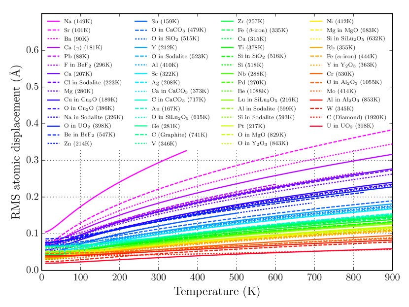
Figure 1: Root-mean-squared atomic displacements in a number of crystals predicted by the Debye model as discussed in the text. The applied Debye temperatures are indicated in parentheses, and curves are terminated at the melting points where relevant.

3 Core framework overview

At its core, all capabilities of the NCrystal toolkit are implemented in an object oriented manner in a C++ library, providing both clearly defined interfaces for clients and internal separation between code implementing physics models, code loading data, and code providing infrastructure needed for integration into final applications. As will be discussed in further detail in Sections 5 and 6, it should be noted that while it is certainly possible to use the C++ classes discussed in the present section directly, typical users are expected to use other more suitable interfaces for their work – employing also a simpler and generic approach to material configuration.

In Figure 2 is shown the most important classes available in the release of NCrystal presented here, along with their internal inheritance relationships. At the root of the tree sits a few infrastructure classes not directly related to actual physics modelling, starting with the universal base class RCBase, which provides reference counted memory management for all derived classes. One level below this sits the CalcBase class, from which all classes actually implementing physics modelling code must inherit. The main feature of CalcBase is currently that it provides derived classes with access to pseudo-random numbers, in a manner which can be configured either globally or separately for each CalcBase instance. In order to do so, each CalcBase instance keeps a reference to an instance of a class deriving from RandomBase – a class which provides a generic interface for pseudo-random number generation. The primary purpose of this setup is to let NCrystal code use external sources of random numbers when embedded into existing frameworks managing their own random number generators, like those discussed in Sections 6.3 and 6.4. If no particular random generator is otherwise enabled, the system will fall back to using a xoroshiro128+ [60] generator implemented in the RandXRSR class.

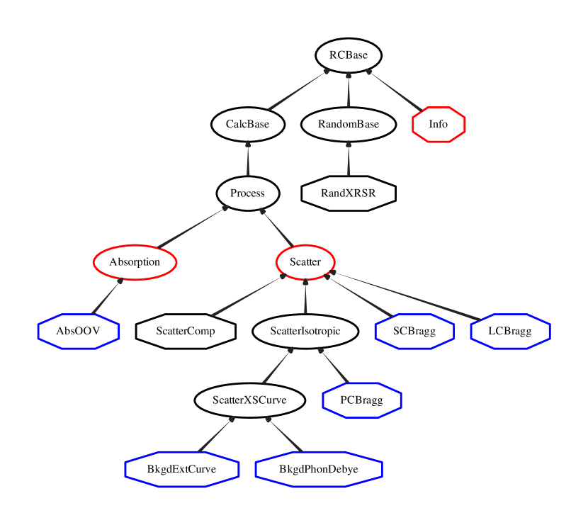
Figure 2: NCrystal class hierarchy. Abstract classes are indicated with rounded edges while concrete classes are shown in octagons. The most important interfaces providing end-user results are indicated in red and final classes providing physics modelling are shown in blue. Internal utility and factory classes are not shown.

Currently, the only class deriving directly from CalcBase is Process. This is an abstract class representing a physics process, specifying a general interface for calculation of cross sections as a function of incident neutron state. The returned cross section values are normalised to the number of atoms in the sample, and the neutron states are specified in terms of kinetic energy ($E_{i}$) and direction ($\hat{k}_{i}$), which is equivalent to providing $\vec{k}_{i}$ but using parameters typically available in general purpose Monte Carlo applications without conversions. Additionally, for reasons of convenience and computational efficiency, it is possible for processes to indicate if they are only relevant for a given energy range (domain), and processes are divided into those that are oriented in the sense that they actually depend on $\hat{k}_{i}$ and those (isotropic) ones that do not. For the latter, one can access the cross section without specifying a direction. For reference, the precise methods available via the Process interface can be seen in Table 1.

Methods available via the Process interface:
bool isOriented() const;
double crossSection(double ekin, const double (&indir)[3] ) const;
double crossSectionNonOriented( double ekin ) const;
void domain(double& ekin_low, double& ekin_high) const;
Additional methods available via the Scatter interface:
void generateScattering( double ekin, const double (&indir)[3],
double (&outdir)[3], double& delta_ekin ) const;
void generateScatteringNonOriented( double ekin, double& angle,
double& delta_ekin ) const;

Table 1: C++ methods provided on the Process and Scatter interface classes.

Two abstract classes further specialise the Process interface, with roles indicated by their names: Absorption and Scatter. The Absorption class does not currently provide any functionality over the Process class, since the current scope of NCrystal does not include any particular description of absorption reactions apart from their cross sections. In principle it would of course be possibly to extend this class in the future, should the need ever arise for NCrystal to be able to model the actual outcome of such events in terms of secondary particles produced.

The Scatter class does on the other hand extend the Process interface, adding methods for random sampling of final states, as can also be seen in Table 1. Specifically, this sampling generates both energy transfers, $E_{f}-E_{i}$, and final direction of the neutron, $\hat{k}_{f}$. In the case of isotropic processes, only the energy transfer and the polar scattering angle, $\theta$, from $\hat{k}_{i}$ to $\hat{k}_{f}$ will depend on the actual physics implemented, and will itself be independent of $\hat{k}_{i}$. The azimuthal scattering angle will be independent and uniformly distributed in $[0,2\pi)$. For isotropic processes, it is thus again possible if desired to avoid the methods with full directional vectors and instead sample energy transfer and polar scatter angle given just the kinetic energy. The specialised base class ScatterIsotropic is provided for developers in order to simplify implementation of isotropic scatter processes. This somewhat complicated design was chosen in order to make it straight-forward to accommodate both oriented and isotropic scatter processes in the same manner, avoiding unnecessary duplication of code and interfaces while still making it possible to retain full computational efficiency allowed by the symmetries in the isotropic cases. The next class in Figure 2, ScatterXSCurve, exists in order to facilitate scatter models which only provide cross sections, adding simple fall-back models for sampling of final states. Rounding up the scattering infrastructure, ScatterComp is a wrapper class playing a special role, representing the composition of multiple Scatter objects into a single one. It is used whenever multiple independent components representing partial cross sections must be combined in order to fully describe the scattering process of interest – such as when a Bragg diffraction component is combined with a component providing inelastic or incoherent scattering. At the bottom of the class hierarchy in Figure 2 sits classes actually implementing physics models of absorption or scattering, shown in blue. They will be discussed in further detail in Section 3.1.

Finally, the Info class is a data structure containing information about crystal structure at the microscopic scale of crystallites. As illustrated in Figure 3, the Info class serves the role of separating sources of crystal definitions from the physics models using the data as input. The data fields available on the Info class are provided in Table 2. Not all input sources will be able to provide all the data fields shown, nor will a particular physics modelling algorithm require all fields to be available. Thus, to ensure maximal flexibility for both providers and consumers of Info objects, all data fields are considered optional. If a given physics algorithm does not find the information it needs, it should simply indicate a configuration error, by throwing an appropriate C++ exception. When configuring materials via the recommended method for end-users (cf. Section 5), the factory code will generally try to avoid triggering undesired errors when the user intent seems obvious: if for instance the input data does not provide any information out of which it would be possible to provide cross sections for inelastic scattering processes, it is most likely that the user is simply only interested in elastic physics and no instantiation of inelastic processes will be attempted.

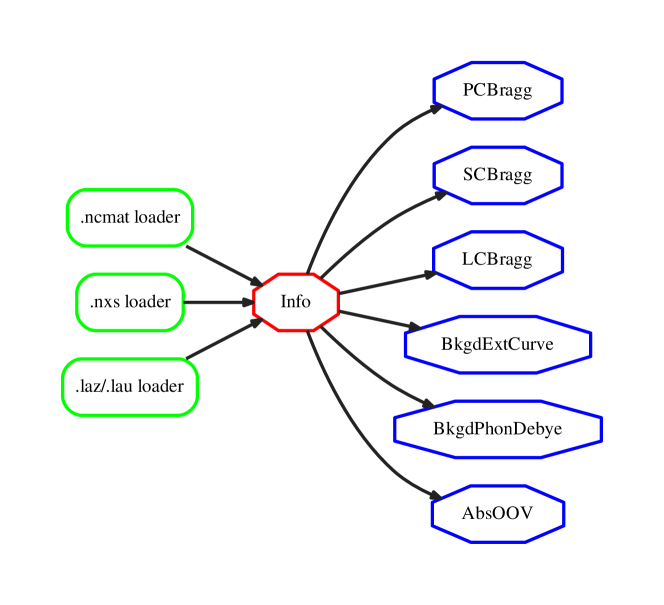
Figure 3: Flow of crystal data in NCrystal. Different factories are responsible for turning crystal definitions from a variety of sources into full-fledged instantiations of the Info class, which is then consumed by various physics models.

Field	Contents	Units
StructureInfo	Basic info about unit cell:
	Lattice parameters ($a$, $b$, $c$, $\alpha$, $\beta$, $\gamma$)	$\text{\,}\mathrm{\SIUnitSymbolAngstrom}\text{/}$, $\text{\,}\mathrm{\SIUnitSymbolDegree}\text{/}$
	Volume	$\text{\,}{\mathrm{\SIUnitSymbolAngstrom}}^{3}\text{/}$
	Number of atoms
	Space group number†
AtomInfo (list)	List of atoms in unit cell, each with:
	Atomic number (Z)
	Number per unit cell
	Per-element Debye temperature†	$\text{\,}\mathrm{K}\text{/}$
	Mean squared displacement†	$\text{\,}\mathrm{\SIUnitSymbolAngstrom}\text{/}$
	List of element positions†
HKLInfo (list)	List of $hkl$ families, each with:
	$hkl$ value (representative)
	$d$-spacing	$\text{\,}\mathrm{\SIUnitSymbolAngstrom}\text{/}$
	Form factor, $|F(\vec{\tau}_{hkl})|^{2}$	$\text{\,}\mathrm{b}\text{/}$
	Multiplicity (family size)
	List of all $hkl$ values in family†
	List of all normals in family†
$d_{\text{cut}}$	Threshold $d$-spacing value for $hkl$ list	$\text{\,}\mathrm{\SIUnitSymbolAngstrom}\text{/}$
$\sigma_{\text{abs}}$	Absorption cross section at $2200\text{\,}\mathrm{m}\mathrm{/}\mathrm{s}$	$\text{\,}\mathrm{b}\text{/}$
$\sigma_{\text{free}}$	Unbound scattering cross section	$\text{\,}\mathrm{b}\text{/}$
$\sigma_{\text{bkgd}}(\lambda)$	Cross section curve for inelastic/incoh.	$$\text{\,}\mathrm{\SIUnitSymbolAngstrom}\text{/}$\to$\text{\,}\mathrm{b}\text{/}$$
	scattering components (function object)
Temperature	Material temperature	$\text{\,}\mathrm{K}\text{/}$
Debye temperature	Global Debye temperature of material	$\text{\,}\mathrm{K}\text{/}$
Density	Material density	$\text{\,}\mathrm{g}\text{/}{\mathrm{cm}}^{3}$

Table 2: Data fields of Info objects. A field can represent either a scalar value or a block of related data, and the availability of all fields is optional. Additionally, some parameters inside block fields might themselves be optional, as indicated with $\dagger$’s. Cross sections are given as per-atom values, averaged over the atoms of the unit cell. An “$hkl$ family” is here a group of $hkl$ indices for which form factors and $d$-spacings have identical values.

This scheme of decoupling data loading code from physics models allows NCrystal to easily support data read from a variety of input files, and makes it simple to add support for additional input sources in the future. If desired, it would even be possible to specify the information directly in program code or load it from a database. Currently supported data sources are discussed in Section 4.

In Listing 1 is shown an example of C++ code loading a crystal definition and constructing objects able to model absorption and scattering in a polycrystalline or powdered material. The example illustrates in practice how some of the classes discussed in this section are used, but also indicates the complexity arising out of the need to provide model-specific parameters. In Section 5, a more convenient method for initialisation and configuration will be introduced.

Listing 1: C++ code loading a crystal definition and creating related NCrystal objects.

⬇

#include "NCrystal/NCrystal.hh"

namespace NC = NCrystal;//alias for convenience

int main() {

//Create crystal Info based on a datafile and other

//parameters (here temperature and d-spacing cutoff):

std::string datafile = "somefile.ncmat";

double temp_kelvin = 400;

double dcutoff_angstrom = 0.5;

const NC::Info * info = NC::loadNCMAT( datafile,

temp_kelvin,

dcutoff_angstrom );

//Compose Scatter and Absorption objects, passing the Info

//object and other parameters as needed:

bool bkgd_thermalise = true;

NC::ScatterComp * scat = new NC::ScatterComp();

scat->addComponent(new NC::PCBragg(info));

scat->addComponent(new NC::BkgdPhonDebye( info,

bkgd_thermalise ));

NC::Absorption * absn = new NC::AbsOOV(info);

// ...

// code here using info, scat and absn pointers

// ...

return 0;

}

3.1 Physics models

At the heart of NCrystal is the actual modelling of specific physics processes, provided via the classes shown with blue outlines in Figure 2. The only modelling of absorption cross sections presently available is provided in the AbsOOV class, which implements the $1/v$ scaling model discussed in Section 2.2, by scaling the value of $\sigma_{\text{abs}}$ given at the reference velocity of $2200\text{\,}\mathrm{m}\mathrm{/}\mathrm{s}$ (cf. Table 2). Despite being implemented with a simple model, absorption cross sections are nonetheless provided in NCrystal for completeness, in order to carry out validation against data from measurements of total cross sections like those presented in Section 4.4 or to facilitate the creation of plugins for Monte Carlo simulations like the one presented in Section 6.4. Additionally, it is important to reiterate that for most nuclear isotopes, the $1/v$ modelling is actually remarkably accurate at thermal neutron energies (cf. Section 2.2).

The remaining physics models all concern scattering processes. Three processes implement the coherent elastic physics of Bragg diffraction discussed in Section 2.3, differing by which distribution of crystallite grains they assume as discussed in Section 2.1. PCBragg implements an ideal powder model, with cross sections given by Eq. 35 and scattering into Debye-Scherrer cones. It can be used to model powders and polycrystalline materials. SCBragg implements a model for single crystals with isotropic Gaussian mosaicity, and LCBragg provides a special anisotropic model of layered crystals similar to pyrolytic graphite. For reasons of scope, the three models of Bragg diffraction will be presented in detail in a future dedicated publication, covering details of both theory, implementation and validation.

Two models currently provide incoherent and inelastic physics: BkgdExtCurve and BkgdPhonDebye. The former is a simple wrapper of externally provided $\sigma_{\text{bkgd}}(\lambda)$ cross section curves (cf. Table 2), and exists mostly for reference, allowing nxslib-provided cross section curves to be exposed via NCrystal when using .nxs files (cf. Section 4.2). Unless selected explicitly, the factories discussed in Section 5 will always prefer the more accurate model provided by BkgdPhonDebye. This improved model relies on the incoherent approximation and the iterative procedure discussed in Section 2.4, and will be presented in detail in a future dedicated publication. In the current release of NCrystal it does not provide any detailed sampling of scatter angles or energy transfers, and hence like BkgdExtCurve it derives from the ScatterXSCurve class. When asked to generate a scattering, ScatterXSCurve will scatter isotropically and either model energy transfers as absent (i.e. elastic), or as “fully thermalising”. In the latter case, the energy of the outgoing neutron will be sampled from a thermal (Maxwell) energy distribution specified solely by the temperature of the material simulated. Both of these choices use well defined distributions, but are clearly lacking in realism. It is the plan to improve this situation in the future, in order to provide a complete and consistent treatment of all components involved in thermal neutron scattering. For most materials, this will be achieved by adopting proper sampling models in BkgdPhonDebye, still based on the currently used iterative procedure for cross section estimation. As already discussed in Section 2.4, it is additionally planned to allow even higher accuracy and reliability when modelling inelastic scattering in select materials, by introducing data-driven models which are able to utilise pre-tabulated scatter-kernels or phonon state densities, if available.

4 Crystal data initialisation

Currently, NCrystal supports the loading of crystal information from four different file formats: the native and recommended .ncmat format which will be introduced in Section 4.1, and the existing .nxs, .laz, and .lau formats which will be discussed in Sections 4.2 and 4.3. The latter formats are mostly supported as a service to the neutron scattering community already using these, for instance in the context of configuring instrument simulations in McStas [12, 13] or VitESS [14, 15]. Support for direct loading of CIF (“Crystallographic Information File”) files [61] was considered as they are readily available in online databases [62, 63], but ultimately abandoned due to the flexible nature of such files, many of which were found in practice to not contain suitable information for the purposes of NCrystal. Manually selected CIF files were, however, read with [64] and used to assemble a library of .ncmat files which is shipped with NCrystal. These files, providing the crystal structures listed in Table 3, first and foremost describe many materials of interest to potential NCrystal users, serving both as a convenient starting point and point of reference. Moreover, the library encompasses six of the seven crystal systems, includes mono- and poly-atomic crystals, and includes materials with large variations in quantities like Debye temperatures, neutron scattering lengths and number of atoms per unit cell. Thus, it provides a convenient ensemble for benchmarking and validating NCrystal code. Additionally, where not prevented for technical reasons like usage of per-element Debye temperatures in poly-atomic systems, .nxs files were automatically generated from the provided .ncmat files. Section 4.4 will describe the validation carried out as concerns both the data files themselves, as well as the code responsible for loading crystal information from them. Naturally, it is fully expected that the list of files in Table 3 will be expanded in the future, in response to requests from the user community.

Crystal	Space group	References	Formats	Validations
Ag	225 (Cubic)	[63, 11135][65][58]	.ncmat, .nxs	N$\overline{\text{T}}$
Al2O3 (Corundum)	167 (Trigonal)	[63, 09327][66]	.ncmat	$\overline{\text{N}}$$\overline{\text{T}}$GF
Al	225 (Cubic)	[63, 11136][65][58]	.ncmat, .nxs	NT
Au	225 (Cubic)	[63, 11140][65][58]	.ncmat, .nxs	N$\overline{\text{T}}$
Ba	229 (Cubic)	[63, 11207][65][58]	.ncmat, .nxs	NF
BeF2 (Be. fluoride)	152 (Trigonal)	[67]	.ncmat	$\overline{\text{N}}$F
Be	194 (Hexagonal)	[63, 11165][65][58]	.ncmat, .nxs	NT
C (Pyr. graphite)	194 (Hexagonal)	[63, 14675][68]	.ncmat	NTF
C (Diamond)	227 (Cubic)	[63, 11242][65][58]	.ncmat, .nxs	NF
CaCO3 (Aragonite)	62 (Orthorhombic)	[63, 06300][69]	.ncmat	$\overline{\text{N}}$GF
Ca	225 (Cubic)	[63, 11141][65][58]	.ncmat, .nxs	N$\overline{\text{T}}$
Ca ($\gamma$-calcium)	229 (Cubic)	[63, 11208][65][58]	.ncmat, .nxs	NF
Cr	229 (Cubic)	[63, 11209][65][58]	.ncmat, .nxs	NT
Cu2O (Cuprite)	224 (Cubic)	[63, 09326][66]	.ncmat	$\overline{\text{N}}$F
Cu	225 (Cubic)	[63, 11145][65][58]	.ncmat, .nxs	NT
Fe ($\alpha$-iron)	229 (Cubic)	[63, 11214][65][58]	.ncmat, .nxs	N$\overline{\text{T}}$
Fe ($\beta$-iron)	229 (Cubic)	[63, 11215][65][58]	.ncmat, .nxs	NF
Ge	227 (Cubic)	[63, 11245][65][58]	.ncmat, .nxs	NT
MgO (Periclase)	225 (Cubic)	[63, 00501][70]	.ncmat	$\overline{\text{N}}$F
Mg	194 (Hexagonal)	[63, 11183][65][58]	.ncmat, .nxs	N$\overline{\text{T}}$
Mo	229 (Cubic)	[63, 11221][65][58]	.ncmat, .nxs	NT
Na	229 (Cubic)	[63, 11223][65][58]	.ncmat, .nxs	NF
Na4Si3Al3O12Cl (Sodalite)	218 (Cubic)	[63, 06211][71]	.ncmat	$\overline{\text{N}}$F
Nb	229 (Cubic)	[63, 11224][65][58]	.ncmat, .nxs	NT
Ni	225 (Cubic)	[63, 11153][65][58]	.ncmat, .nxs	NT
Pb	225 (Cubic)	[63, 11154][65][58]	.ncmat, .nxs	N$\overline{\text{T}}$
Pd	225 (Cubic)	[63, 11155][65][58]	.ncmat, .nxs	N$\overline{\text{T}}$
Pt	225 (Cubic)	[63, 11157][65][58]	.ncmat, .nxs	N$\overline{\text{T}}$
Rb	229 (Cubic)	[63, 11228][65][58]	.ncmat, .nxs	NF
Sc	194 (Hexagonal)	[63, 11192][65][58]	.ncmat, .nxs	N$\overline{\text{T}}$
SiLu2O5	15 (Monoclinic)	[72]	.ncmat	$\overline{\text{N}}$RF
SiO2 (Quartz)	154 (Trigonal)	[63, 06212][71]	.ncmat	$\overline{\text{N}}$GF
Si	227 (Cubic)	[63, 11243][65][58]	.ncmat, .nxs	NT
Sn	141 (Tetragonal)	[63, 11248][65][58]	.ncmat, .nxs	NT
Sr	225 (Cubic)	[63, 11161][65][58]	.ncmat, .nxs	NF
Ti	194 (Hexagonal)	[63, 11195][65][58]	.ncmat, .nxs	N$\overline{\text{T}}$
UO2 (Uraninite)	225 (Cubic)	[63, 11728][65][59]	.ncmat, .nxs	NT
V	229 (Cubic)	[63, 11235][65][58]	.ncmat, .nxs	N$\overline{\text{T}}$
W	229 (Cubic)	[63, 11236][65][58]	.ncmat, .nxs	N$\overline{\text{T}}$
Y2O3 (Ytr. oxide)	206 (Cubic)	[73]	.ncmat	$\overline{\text{N}}$GF
Y	194 (Hexagonal)	[63, 11199][65][58]	.ncmat, .nxs	NT
Zn	194 (Hexagonal)	[63, 11200][65][58]	.ncmat, .nxs	NT
Zr	194 (Hexagonal)	[63, 11201][65][58]	.ncmat, .nxs	N$\overline{\text{T}}$

Table 3: Crystal definitions currently shipped with NCrystal. Structures and Debye temperatures were obtained from the listed references, with specific database IDs for [63]. The last column indicates validations, as discussed in Section 4.4: checks with nxslib of symmetries and form factors (N,$\overline{\text{N}}$); with experimental total cross sections (T,$\overline{\text{T}}$); with standard refinement software on simulated powder patterns (G,F); with measured form factors (R).

4.1 NCrystal material files (.ncmat)

Intended to be straight-forward to parse algorithmically, while at the same time being directly legible to scientists with crystallographic knowledge, the layout of NCrystal material files is deliberately kept both simple and intuitive, as illustrated with the sample file in Listing 2. These simple text files always begin with the keyword NCMAT and the version of the format. Next comes optionally a number of #-prefixed lines with free-form comments, intended primarily as a place to document the origin, purpose or suitability of the file. The data itself follows after this introduction, and is placed in four clearly denoted sections as shown in the listing. The @CELL and @ATOMPOSITIONS sections define the unit cell layout directly, and the definition must be compatible with the space group number which can optionally be provided in the @SPACEGROUP section. Finally, the @DEBYETEMPERATURE section contains the effective Debye temperature of the crystal (cf. Section 2.5) – either a single global value, or as per-element values, indicated with the name of each element (for mono-atomic crystals, there is of course no difference between specifying a per-element or a global value). Where relevant, values are specified in units of $\mathrm{\SIUnitSymbolAngstrom}\text{/}$, $\mathrm{K}\text{/}$ and degrees for lengths, temperature and angles respectively.

Listing 2: Sample .ncmat file defining the face-centred cubic structure of a pure aluminium crystal, with lattice lengths of $4.049\,58\text{\,}\mathrm{\SIUnitSymbolAngstrom}\text{/}$ and a Debye temperature of $410.35\text{\,}\mathrm{K}\text{/}$.

⬇

NCMAT v1

#Converted from the CIF file of the entry 0011136 in the AMCSD

#reference: Wyckoff R W G, Crystal Structures, vol. 1, p. 7-83,

#1963. The Debye temperature is derived from the Debye-Waller

#factor at 293K compiled in the supplement of Acta Cryst., A52,

#p. 456-470, 1996.

@CELL

lengths 4.04958 4.04958 4.04958

angles 90. 90. 90.

@SPACEGROUP

225

@ATOMPOSITIONS

Al 0. 0.5 0.5

Al 0. 0. 0.

Al 0.5 0.5 0.

Al 0.5 0. 0.5

@DEBYETEMPERATURE

Al 410.35

The atomic positions are specified using relative lattice coordinates (cf. Eq. 1), and the name of an element is also required at each such position. It is not necessary, nor currently possible, to specify element-specific data such as masses, cross sections or scattering lengths. Instead, NCrystal currently includes an internal database of such numbers for all natural elements with $Z\leq 92$, based on [74, 75, 76]. Although somewhat inflexible, this scheme provides a high level of convenience, consistency and robustness by significantly lowering the amount of parameters required in each .ncmat file. It is envisioned that a future version of NCrystal would support more specialised use-cases by supporting not only the optional specification of element- and isotope-specific data in .ncmat files, but also to allow for specification of features like chemical disorder, impurities, doping or enrichment.

With the information parsed directly from the .ncmat file and the specification of a material temperature, the remaining information shown in Table 2 will be derived numerically at initialisation time (with the exception of $\sigma_{\text{bkgd}}(\lambda)$ which is not relevant for .ncmat files). The involved calculations are mostly trivial, with one exception being the atomic mean-squared displacements which are calculated based on the isotropic Debye model discussed in Section 2.5. The other exception is the creation of the $hkl$ lists (HKLInfo) and the associated $d$-spacing threshold, $d_{\text{cut}}$. For a given value of $d_{\text{cut}}$, all $hkl$ points in the reciprocal lattice with $d_{hkl}\geq{d}_{\text{cut}}$ are considered. The number of such points can be considerable, as shown in Figure 4, and considerable care is taken to control the initialisation time. At each given $hkl$ point the squared form factors, $|F(\vec{\tau}_{hkl})|^{2}$, are calculated directly via a numerical evaluation of Eq. 25, requiring relatively expensive sine and cosine function evaluations with the phase specific to each atomic position, $\vec{\tau}_{hkl}\cdot\vec{p}_{i}$. Naturally, the $\overline{b_{i}}{e}^{-W_{i}(\vec{Q})}$ factors are computed just once and reused, and half of the $hkl$ points are dealt with by using the symmetry $|F(\vec{\tau}_{hkl})|^{2}=|F(-\vec{\tau}_{hkl})|^{2}$. Additionally, entries with squared form factors less than a fixed threshold value of $f_{\text{cut}}=${10}^{-5}\text{\,}\mathrm{b}\text{/}$$ are discarded. This keeps forbidden $hkl$ entries out of the final lists, i.e. those which for reasons of symmetry should have vanishing form factors in the strict mathematical sense, but which nevertheless acquire tiny non-zero but negligible values during the numerical evaluations. More importantly, the non-zero value of $f_{\text{cut}}$ enables significant improvements in initialisation time through an early-abort technique. Specifically, an upper bound on the squared form factor value can be calculated without any looping over atom positions or expensive trigonometric function evaluations, by replacing all involved sines and cosines calls with $1$. This can make it possible to predict without expensive calculations that a value $f_{\text{cut}}$ is unreachable. In fact, only $hkl$ points near the origin of the reciprocal lattice need detailed consideration, because the Debye-Waller factors suppress entries with smaller $d$-spacings (cf. Eq. 40): $\exp(-W_{i}(\vec{\tau}_{hkl}))=\exp(-2\pi^{2}\delta^{2}_{i}/d^{2}_{hkl})$. In particular, it means that the time required for $hkl$ list initialisation practically tends towards a constant as $d_{\text{cut}}$ is decreased to ever smaller values. This behaviour is much preferable to the $\mathcal{O}(1/d^{3}_{\text{cut}})$ behaviour of an implementation without such an early-abort.

In addition to the calculation of squared form-factors at all considered $hkl$ points, points must also be sorted into families of points sharing $d$-spacing and squared form-factor values. This is done with a map-based $\mathcal{O}(\log(d_{\text{cut}}))$ algorithm. All together, the final result is an $hkl$ list initialisation algorithm which is fast enough that the trade-off between accuracy and initialisation time inherent in the choice of $d_{\text{cut}}$ is not very severe.

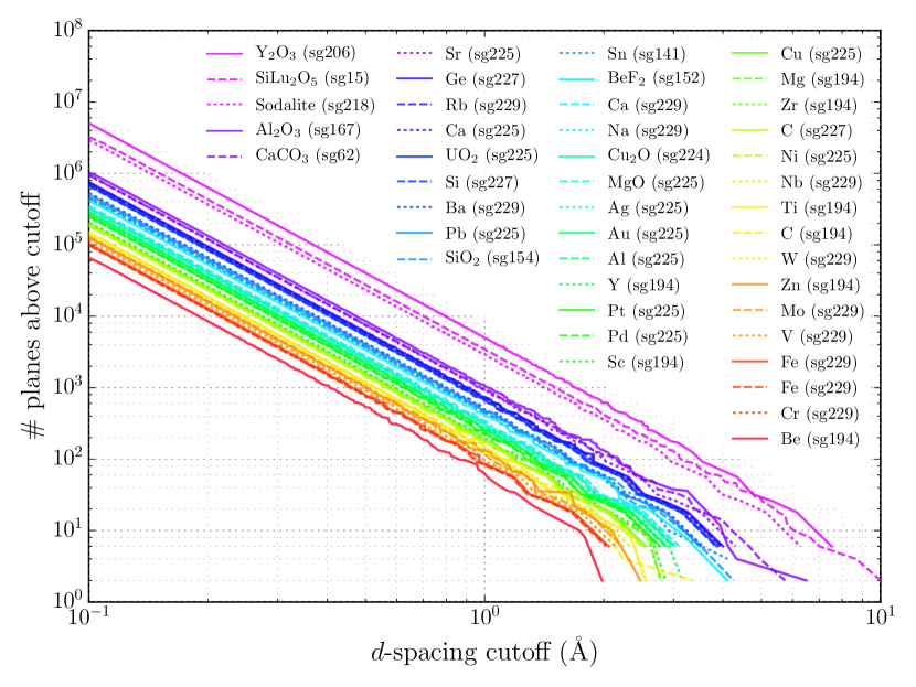
Figure 4: Number of $hkl$ planes above a given $d$-spacing threshold for crystal structures in the NCrystal data library.

The value of $d_{\text{cut}}$ can always be set directly by the users, but in order to determine appropriate default values for the majority of users who are not expected to do so, the impact on Bragg diffraction cross sections in the powder approximation (cf. Eq. 35) was investigated. Although most powder diffraction experiments would concentrate on wavelengths longer than $2d_{\text{cut}}$, and therefore not be directly affected by it, the total cross section for diffraction in a powder is still a meaningful benchmark. After all, if a too high cut-off value is chosen, too many planes would be left out and the total cross section would be underestimated at shorter wavelengths – with corresponding degradation of realism in a simulation of for instance beam filters or shielding based on powders or polycrystalline materials. Thus, Figure 5 shows the relative impact of $d_{\text{cut}}$ on the cross section in the limiting case $\lambda\rightarrow 0$. The impact levels gauged in this limit are clearly very conservative, since at this wavelength all omitted planes satisfy Eq. 32 resulting in a large relative impact, while the factor of $\lambda^{2}$ in Eq. 35 removes any absolute impact. Still, to be conservative, a fairly aggressive default value of $d_{\text{cut}}=$0.1\text{\,}\mathrm{\SIUnitSymbolAngstrom}\text{/}$$ was chosen. This is a sensible choice, since the typical initialisation time of most materials with this value range from a few milliseconds to approximately one second, depending on unit cell complexity. Two of the tested materials in the data library stood out, however, with initialisation times of $6\text{\,}\mathrm{s}\text{/}$ (SiLu₂O₅) and $31\text{\,}\mathrm{s}\text{/}$ (Y₂O₃) respectively. These crystal structures are distinguished by their large unit cell volumes and number of atoms per unit cell, 64 and 80 respectively. In order to keep default load times at approximately $1\text{\,}\mathrm{s}\text{/}$ or less, a number which is unlikely to cause concern for casual users, the default value is raised to $d_{\text{cut}}=$0.25\text{\,}\mathrm{\SIUnitSymbolAngstrom}\text{/}$$ for materials with more than 40 atoms in the unit cell.

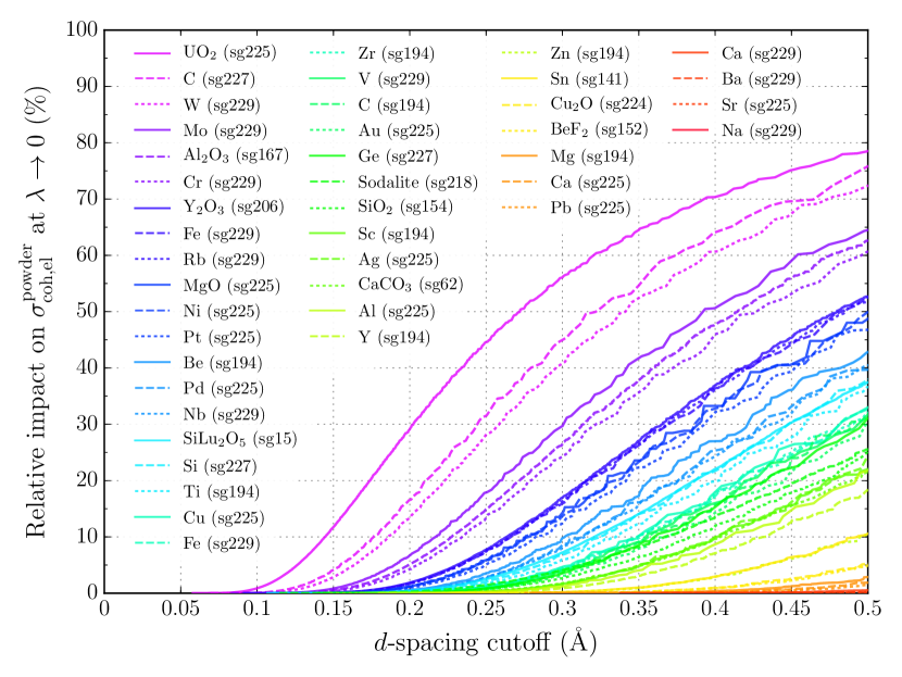
Figure 5: Relative impact in the short-wavelength limit of $d$-spacing threshold on the cross section for Bragg diffraction in a powder, for crystal structures in the NCrystal data library.

The resulting impact on the cross section curve of both thresholds applied by default, $f_{\text{cut}}=${10}^{-5}\text{\,}\mathrm{b}\text{/}$$ and $d_{\text{cut}}=$0.1\text{\,}\mathrm{\SIUnitSymbolAngstrom}\text{/}$$ or $0.25\text{\,}\mathrm{\SIUnitSymbolAngstrom}\text{/}$, is shown in Figure 6. For most materials the effect is completely negligible, and even in the worst case of yttrium-oxide, the effect exists only at very short wavelengths and is hardly noticeable.

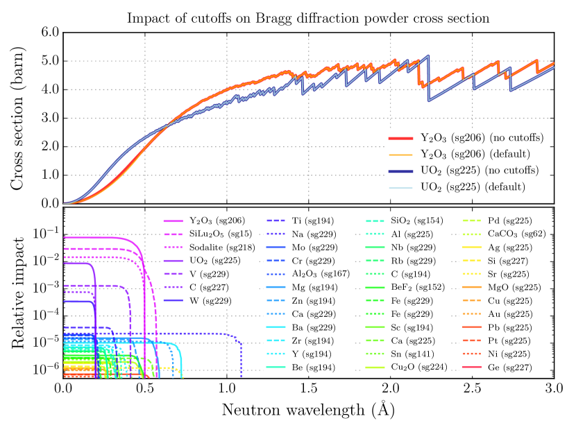
Figure 6: Impact of the default thresholds ($f_{\text{cut}}=${10}^{-5}\text{\,}\mathrm{b}\text{/}$$ and $d_{\text{cut}}=$0.1\text{\,}\mathrm{\SIUnitSymbolAngstrom}\text{/}$$ or $0.25\text{\,}\mathrm{\SIUnitSymbolAngstrom}\text{/}$) on the cross section for Bragg diffraction in a powder, for crystal structures in the NCrystal data library. The plot on top compares cross section curves directly for two of the most affected materials, while the plot below shows the relative impact for all structures in the NCrystal data library.

4.2 .nxs file loader

Routines in the nxs library [30, 77, 78], used in McStas [12, 13], VitESS [14, 15] and NXSG4 [31] to provide cross sections in crystal powders, comes with an associated text-based file format for crystal structure definition, recognised by the extension .nxs. The file format, described in [31], contains information similar to that in the .ncmat file of Listing 2 with a few notable differences. The first one is that element-specific cross sections and masses must be specified directly in the files themselves, and the second is that the files do not contain the full list of atomic positions in the unit cell, but rather just the Wyckoff positions of the atoms. Finally, only a global Debye temperature can be specified, meaning that per-element Debye Temperatures in poly-atomic systems are unsupported. Upon loading the file, the nxs library creates the full list of atomic positions in the unit cell by application of the relevant symmetry operators of the specified crystal space group, which is carried out through an internal dependency on the SgInfo [79] library. Support of the .nxs format in NCrystal thus introduce dependencies on these two external libraries, each with their own unique open source license. In order to ensure that only users actually interested in .nxs file support would be exposed to these extra license requirements, the NCrystal code implementing the support for .nxs file loading is kept clearly separated from the rest, and it is straight-forward to build NCrystal without it.

Upon loading .nxs files, most information shown in Table 2 will be loaded directly from the input file. The $hkl$ lists in the HKLInfo section are, however, provided by calculations in the nxs library, and are not calculated directly in NCrystal code. On one hand this ensures that users loading .nxs files will get the exact same form factors when loading their files with NCrystal as when loading them elsewhere. More importantly, however, it makes it possible to perform meaningful cross checks of the results of loading equivalent .ncmat and .nxs files by comparing the resulting form factors with those resulting from loading an equivalent .nxs file. As the nxs library evaluates Debye-Waller factors using a model [80] which is based on the same underlying approximations of isotropic displacements and the Debye Model (cf. Section 2.5), the resulting form factors should be directly comparable. However, as the $hkl$ list creation in the nxs library relies on application of space group symmetries, employing selection rules and starting from Wyckoff positions rather than the full list of atomic positions, such comparisons are highly non-trivial, validating both the compared files and the code loading them. The result of such validations are discussed in Section 4.4.

An important detail in the construction of $hkl$ lists is that the nxs library does not directly support a specification of a $d$-spacing threshold, instead limiting the range of Miller indices probed by specification of a parameter $N_{\text{max}}$, resulting in the consideration of all $hkl$ points for which $|h|,|k|,|l|\leq{N}_{\text{max}}$. Consequently, the $d$-spacing threshold is implemented on the NCrystal side by first calculating the value of $N_{\text{max}}$ needed to contain all points withing $d_{\text{cut}}$, and subsequently ignoring all entries inevitably generated with a $d$-spacing beyond this value. As the nxs library code for grouping $hkl$ entries into families is implemented with a relatively slow linear algorithm (resulting in an overall algorithmic complexity of $\mathcal{O}(N^{4}_{\text{max}})$), the $d_{\text{cut}}$ value selected by default for .nxs files is somewhat higher than for .ncmat files. It is chosen so as to correspond to $N_{\text{max}}=20$ but with $d_{\text{cut}}$ at most $0.5\text{\,}\mathrm{\SIUnitSymbolAngstrom}\text{/}$ and at least $0.1\text{\,}\mathrm{\SIUnitSymbolAngstrom}\text{/}$. To prevent perceived programme lockups, it will result in an error if a user requests a $d_{\text{cut}}$ value which requires $N_{\text{max}}>50$.

Another important point is that the nxs code was not written to support single crystal modelling, and therefore the loaded HKLInfo objects will contain no lists of normals or $hkl$ indices. However, when $hkl$ family composition corresponds to symmetry equivalence groups (as is indeed the case for .nxs files), the NCrystal single crystal code is able to reconstruct such lists of normals on demand if absent, and it will therefore still be possible to use .nxs files for single crystal simulations in NCrystal. Finally, the nxs library provides estimates of inelastic/incoherent scattering cross sections based on various empirical formulas, and these will be provided in the $\sigma_{\text{bkgd}}(\lambda)$ field of Info objects when an .nxs file is loaded. By default, the cross section curve provided is similar to the one discussed in [31], representing an ad hoc combination of empirical formulas due to Freund [49] and Cassels [50]. As discussed in Section 3.1, these curves are provided for reference: the native NCrystal algorithms provide more robust predictions for inelastic/incoherent cross sections and is used by default also when working with .nxs files.

4.3 .laz and .lau file loader

Due to the widespread usage in various McStas components for modelling of Bragg diffraction, NCrystal also supports the loading of .laz file from [81] and .lau files from [82]. Both of these very similar text-based file formats can be generated from a CIF file by the cif2hkl application, part of iFit [83], and their most notable feature is that they directly contain $hkl$ lists with $d$-spacings and form factors. Typically, .laz files are used in the context of powder diffraction, while .lau files can be used to deal with single crystal diffraction as well. This distinction implies that the latter files are larger, since they break down each $hkl$ family into multiple lines of data, in order to provide enough information that all plane normals associated with a given family can be directly inferred.

The NCrystal code loading such files is rather simple, since no special calculations are needed to fill the HKLInfo section. By default, no thresholds are applied upon loading the $hkl$ information from the file, but if desired it is of course possible to specify a custom $d$-spacing threshold in order to ignore some $hkl$ families in the file. Other information in Table 2 loaded from information at the beginning of the files are StructureInfo, $\sigma_{\text{abs}}$, and density. Finally, it is also possible to specify the temperature when loading the file, but it is important to note that since form factors are hard-coded in the file itself, their values are unaffected by the actual value provided. All in all, the loaded information is sufficient for modelling of Bragg diffraction, but absent is information which could be used to model inelastic or incoherent components. Thus, the factories described in Section 5 will create processes without such components for .laz or .lau files.

4.4 Validation

In order to simultaneously validate not only the code responsible for initialising crystal structure information from .ncmat and .nxs files, but also the individual data files provided with NCrystal, multiple approaches were pursued. One particular concern is the code responsible for creating $hkl$ lists with $d$-spacings and squared form factors from .ncmat files. Another is the fact that the crystal symmetry in .ncmat files is contained implicitly in the full list of atomic unit cell positions, as opposed to .nxs or CIF files in which the symmetry is expressed explicitly in terms of space group number and Wyckoff positions. The optional inclusion of the space group number in .ncmat files is mostly cosmetic, and there is currently no guarantee that the indicated space group actually corresponds to the symmetries expressed by the unit cell shape and atomic position.

The first validation carried out for all files requires that the atomic positions in a given .ncmat file are compatible with those generated by nxslib from the Wyckoff positions in the corresponding .nxs file – which behind the scenes implements symmetry operations for the indicated space group via the SgInfo library. Next, as discussed in Section 4.2, the $hkl$ lists created from the two files are also compared systematically. This validates the Debye model and direct approach utilised in the custom $hkl$ list creation code used for .ncmat files against the corresponding but different implementation in nxslib, which relies on symmetry information from the SgInfo library for selection rules and multiplicities. All provided files were validated in this manner, as indicated with N or $\overline{\text{N}}$ in the last column of Table 3. Files marked with $\overline{\text{N}}$ are poly-atomic crystals with per-element Debye temperatures, which is not supported in .nxs files and which accordingly had to be compared using files in which a global Debye temperature was substituted.

Next, the $hkl$ lists created from .ncmat files are validated again by using them to generate artificial powder diffraction spectrums and testing them with software which is normally used to decode crystal structures from such spectrums at real powder diffraction experiments. First, a simple neutron diffraction instrument was simulated with McStas (cf. Section 6.4), using NCrystal and the relevant .ncmat file to model a crystal powder sample. As a result, a powder spectrum was produced for each of the four tested materials – marked with G in the last column of Table 3. These spectra were then used as input to GSAS-II [84], which in all cases managed to recover the crystal structure which was present in the original CIF file from which the relevant .ncmat file was produced. As an example, Figure 7 shows a refinement for a powder spectrum with $9.1\text{\times}{10}^{7}$ simulated neutrons collected in the detector array after interaction with a sapphire sample, and Table 4 shows the corresponding parameters extracted by GSAS-II, which in addition to space group and atomic (Wyckoff) positions also include atomic mean-squared displacements. The goodness-of-fit is provided by GSAS-II in terms of $R$-factor, which in all cases was less than 1.9%, indicating a very high degree of compatibility. Due to the usage of a full-scale simulation with actual NCrystal components enabled, these comparisons incidentally validate features of NCrystal beyond just the initialisation of crystal structure information – but dedicated future publications will document additional validations performed for these more thoroughly.

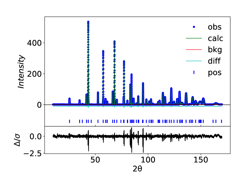
Figure 7: Comparison of sapphire (corundum) powder diffraction pattern simulated by McStas and NCrystal (“obs”) and refined curves from GSAS-II. Refined peak positions are shown in the middle section of the plot and differences (normalised to peak widths) are shown at the bottom. Plot generated by GSAS-II.

	Original	Refined
Lattice $a$ ($\text{\,}\mathrm{\SIUnitSymbolAngstrom}\text{/}$)	4.757	4.75701
Lattice $c$ ($\text{\,}\mathrm{\SIUnitSymbolAngstrom}\text{/}$)	12.9877	12.98773
Al position $x$	0.0	0.00000
Al position $y$	0.0	0.00000
Al position $z$	0.35218	0.35221
O position $x$	0.30625	0.30613
O position $y$	0.0	0.00000
O position $z$	0.25	0.25000
Al MSD ($\text{\,}{\mathrm{\SIUnitSymbolAngstrom}}^{2}\text{/}$)	0.002644	0.00259
O MSD ($\text{\,}{\mathrm{\SIUnitSymbolAngstrom}}^{2}\text{/}$)	0.003167	0.00305
$R$-factor		0.82%

Table 4: Original parameters and refined results from GSAS-II for sapphire (corundum).

In addition to performing a full-blown instrument simulation with McStas, an idealised diffraction spectrum for a given neutron wavelength can be constructed directly from the $d$-spacings, multiplicities and squared form factors in a given $hkl$ list by referring to Eqs. 33 and 35. Furthermore, geometrical coverage of a typical array of detector tubes at a powder diffractometer is accounted for by the introduction of an acceptance factor of $1/\sin\theta$ – and all other effects related to sample size, beam spread and divergence, etc. are modelled in a simplistic manner by replacing the ideal $\delta$-function line shapes with Gaussian distributions of $0.1\text{\,}\mathrm{\SIUnitSymbolDegree}\text{/}$ fixed width. Despite the simplicity, the resulting artificial powder spectra are sufficiently realistic that it is possible to extract the crystal structure from them using FullProf [85]. For the 17 materials tested in this manner, marked with F in the last column of Table 3, FullProf was able to precisely recover their crystal structures – returning $R$-factors which were in all cases better than 2.7%. Figure 8 shows an example of a powder spectrum fitted with FullProf and Table 5 the corresponding extracted parameters.

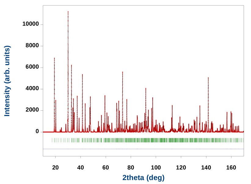
Figure 8: Comparison of artificial aragonite (CaCO₃) powder diffraction pattern constructed based on NCrystal $hkl$ lists (red) and refined curves from FullProf (black). Below are shown refined peak positions (green) and differences between input and refined patterns (blue). Plot generated by FullProf.

	Original	Refined
Lattice $a$ ($\text{\,}\mathrm{\SIUnitSymbolAngstrom}\text{/}$)	4.96062	4.960621
Lattice $b$ ($\text{\,}\mathrm{\SIUnitSymbolAngstrom}\text{/}$)	7.97006	7.970061
Lattice $c$ ($\text{\,}\mathrm{\SIUnitSymbolAngstrom}\text{/}$)	5.74181	5.741809
Ca position $x$	0.25000	0.25000
Ca position $y$	0.41500	0.41500
Ca position $z$	0.75960	0.75960
C position $x$	0.25000	0.25000
C position $y$	0.76190	0.76190
C position $z$	-0.08490	-0.08490
Oa position $x$	0.25000	0.25000
Oa position $y$	0.92240	0.92240
Oa position $z$	-0.09560	-0.09560
Ob position $x$	0.47380	0.47380
Ob position $y$	0.68040	0.68040
Ob position $z$	-0.08710	-0.08710
Ca MSD ($\text{\,}{\mathrm{\SIUnitSymbolAngstrom}}^{2}\text{/}$)	0.0079889	0.00800
C MSD ($\text{\,}{\mathrm{\SIUnitSymbolAngstrom}}^{2}\text{/}$)	0.007991	0.00799
Oa MSD ($\text{\,}{\mathrm{\SIUnitSymbolAngstrom}}^{2}\text{/}$)	0.0124836	0.012482
Ob MSD ($\text{\,}{\mathrm{\SIUnitSymbolAngstrom}}^{2}\text{/}$)	0.0124836	0.012482
$R$-factor		1.96%

Table 5: Original parameters and refined results from FullProf for aragonite.

As another independent validation of squared form factor predictions, measured and refined values for the only monoclinic crystal structure in the considered files (dilutetium silicon pentaoxide, SiLu₂O₅) were taken from [72] (entry 2012009 in [62]), and directly compared against the ones predicted by NCrystal. The result for $d$-spacings larger than $1.5\text{\,}\mathrm{\SIUnitSymbolAngstrom}\text{/}$ is shown in Figure 9, indicating a good agreement. Accordingly, this material is marked with R in the last column of Table 3.

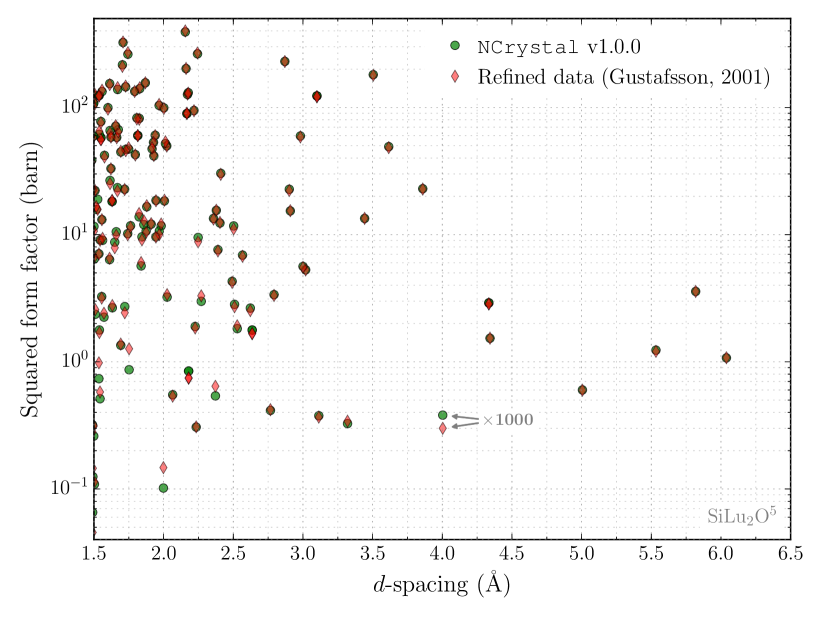
Figure 9: Refined measured squared form factors for monoclinic dilutetium silicon pentaoxide (SiLu₂O₅) [72] compared against those predicted by NCrystal. Note that for visualisation purposes, the weak reflection plane at approximately $4.0\text{\,}\mathrm{\SIUnitSymbolAngstrom}\text{/}$ is shown after multiplication with a factor of 1000.

As a final validation, experimental measurements of energy-dependent total cross sections were obtained from EXFOR [86] where available and tested against predictions from NCrystal. This tests not only .ncmat files and the associated crystal initialisation code, but also partly the implemented physics processes for powders. Most materials were validated in this manner, as indicated with T or $\overline{\text{T}}$ in the last column of Table 3. Where files are marked with $\overline{\text{T}}$, it indicates a rather weak validation of the resulting Bragg edges – either due to low quality data or because that material has a relatively weak coherent elastic component, making the cross section dominated by inelastic or absorption physics. For reasons of space, all resulting validation plots are provided on the Data Library sub-section of [34], with just a few examples included here.

First, Figures 10, 11, and 12 shows comparisons for molybdenum, nickel, and zinc respectively. In all cases, some experimental data sets clearly support the predicted cross sections, but occasionally some data sets provide inconsistent results – in mutual contradiction with not only NCrystal but also other data sets. This underlines the inherent difficulty in performing such validations with pre-existing measurements which might have been performed under different or unclear conditions, with textured samples, etc. Nonetheless, the general agreement with the predictions of NCrystal is clear – and it is interesting to note that it is particularly good for the magnetic material, Nickel. This seems to support the validity of ignoring magnetic interactions in the modelling, as long as both the sample and the incident neutrons themselves are unpolarised. Figure 13 shows another good agreement, this time for a poly-atomic crystal: uranium oxide. Finally, the plot for tin in Figure 14 is interesting in that it confirms a good agreement of Bragg edges and single phonon scattering (despite some unclear result from one data set from an unpublished measurement which could be due to texture). But around $1.3\text{\,}\mathrm{eV}\text{/}$, effects of a nuclear resonance can be seen, which is not currently included in the modelling provided by NCrystal.

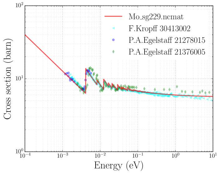
Figure 10: Validation of the total interaction cross section of molybdenum with experimental data from EXFOR [86].

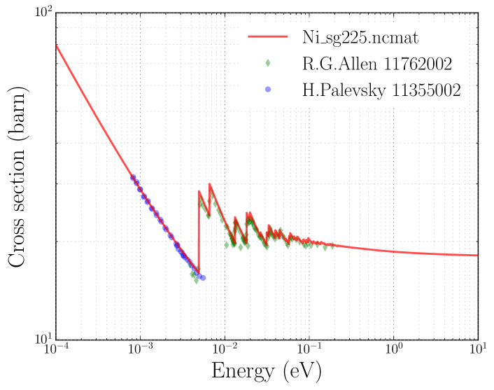
Figure 11: Validation of the total interaction cross section of nickel with experimental data from EXFOR [86].

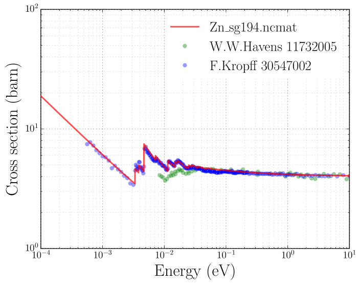
Figure 12: Validation of the total interaction cross section of zinc with experimental data from EXFOR [86].

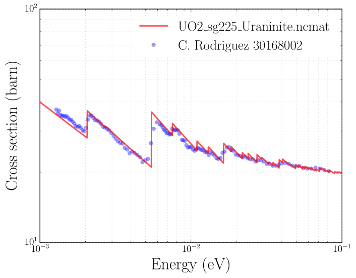
Figure 13: Validation of the total interaction cross section of uranium oxide with experimental data from EXFOR [86].

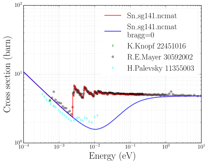
Figure 14: Validation of the total interaction cross section of tin with experimental data from EXFOR [86].

5 Factories and unified configuration

The object oriented implementation of NCrystal in a C++ class hierarchy described in Section 3, provide a high degree of flexibility. This flexibility is an advantage for experts wishing to extend or customise NCrystal, benefiting from low-level access to the various classes and utilities exposed to developers as part of the NCrystal API. However, as demonstrated by the example in Listing 1, this flexibility comes at a cost of complexity which it is desirable to contain. Not only in order to make the usage of NCrystal simpler and less error prone for non-expert users, but also because it is possible to use NCrystal in a variety of different contexts, including several different programming languages and Monte Carlo simulation frameworks as discussed in Section 6. The burden of having to expose, support, document, validate and maintain all customisation options of the core C++ class library in all of these would be highly non-trivial.

Thus, a simplified method for high-level material configuration was adapted for NCrystal and employed in a consistent manner across all supported interfaces and plugins. Specifically, it takes the form of a simple string in which the name of a data file is combined with other parameters as needed. Not only is it technically trivial to accept and pass around such a string in essentially any programming language or user interface, but it is also by definition easily persistifiable and shareable between different users and frameworks. Furthermore, as NCrystal evolves and new material parameters are introduced, existing interfaces and plugins will not require corresponding updates, since they will simply continue to pass along any specified strings to the NCrystal library just as before. The strings are composed according to the following syntax, in which a file name is optionally followed by a semicolon separated list of parameter assignments:

<FILENAME>[;ignorefilecfg][;PARNAME1=VAL1][..][;PARNAMEN=VALN]

Unless the filename is given as an absolute path, NCrystal will first search the current working directory for the data file, then any directory indicated with the environment variable NCRYSTAL_DATADIR, before finally looking in the directory where data files from the data library shipped with NCrystal itself were copied as part of the NCrystal installation procedure. The optional and rarely used ignorefilecfg keyword indicates to NCrystal that it should not search the data files themselves for additional parameter settings. This is needed, because NCrystal allows users to embed default parameter values directly inside the input files (usually in comments), by placing them inside square braces following the keyword NCRYSTALMATCFG. Currently, the only data file in the data library shipped with NCrystal employing this is the file C_sg194_pyrolytic_graphite.ncmat, which contains a comment embedding the following contents:

NCRYSTALMATCFG[lcaxis=0,0,1]

Due to this, the configuration of a single crystal material from that file will result in the anisotropic mosaicity distribution appropriate for pyrolytic graphite to be used rather than the standard isotropic one.

Table 6 documents the configuration parameters most likely to be of interest to typical NCrystal users, but for clarity a few example strings and their implications will be presented in the following.

Parameter	Default	Description	Units (†=default)
temp	$293.15\text{\,}\mathrm{K}\text{/}$	Temperature of material.	K†, C, F
dcutoff	$0$	Value of $d$-spacing threshold, $d_{\text{cut}}$. A value of 0 im-	Aa†, nm, mm, cm, m
		plies automatic threshold selection.
bragg	true	Disable to exclude Bragg diffraction.
bkgd	"best"	Influence incoherent/inelastic models chosen by fac-
		tories. The default, "best", implies most realistic
		available model, while a value of "none" or "0" ex-
		cludes such processes. Other values allow advanced
		users to select or tune models.
Powders only:
packfact	$1.0$	Powder packing factor.
Single crystals only:
mos		Gaussian spread in mosaic crystals (FWHM).	rad†, deg, arcmin, arcsec
dir1		Primary orientation of crystal given by specifying
		directions in both crystal and lab frames with the
		syntax: "@crys:cx,cy,cz@lab:lx,ly,lz".
		Alternatively, the crystal direction can be specified
		in reciprocal lattice space rather than direct space
		as "@crys_hkl:ch,ck,cl@lab:lx,ly,lz".
dir2		Secondary orientation of crystal, specified using the
		same syntax as for the dir1 parameter. Only com-
		ponents of dir2 orthogonal to dir1 will actually
		influence the orientation (but see dirtol).
dirtol	${10}^{-4}\text{\,}\mathrm{rad}\text{/}$	Specification of dir1 and dir2 are accepted only if	rad†, deg, arcmin, arcsec
		the angle between dir1 and dir2 is similar in crys-
		tal and lab frames within this tolerance.
lcaxis		Symmetry axis of anisotropic layered crystals simi-
		lar to pyrolytic graphite (as vector, e.g. "0,0,1").

Table 6: Some of the most important parameters available in NCrystal configuration strings.

• "Al_sg225.ncmat", "Al_sg225.nxs", or "Al.laz"
  Polycrystalline or powdered aluminium at room temperature, using appropriate code for loading .ncmat, .nxs or .laz files respectively. Although in principle representing the same material, the realism will depend on the type of input file, as NCrystal automatically selects the most realistic modelling possible while also considering issues like load times. In this particular case, the scattering models based on the .laz file will not contain any incoherent or inelastic components, and the Bragg diffraction based on the .nxs file will contain fewer reflection planes at shorter $d$-spacings than the one based on the .ncmat file (cf. Section 4.2).

• "Be_sg194.ncmat;temp=100K"
  Polycrystalline or powdered beryllium at a low temperature, useful for modelling of beryllium filters.

• "Be_sg194.ncmat;temp=100K;bkgd=phonondebye:elastic"
  The same beryllium, but forcing the modelling of inelastic scattering with the BkgdPhonDebye class to neglect energy transfers (cf. Section 3.1).

• "Be_sg194.ncmat;bkgd=0;temp=100K"
  The same beryllium again, but this time the only scattering being modelled is that of Bragg diffraction. While clearly decreasing the modelled realism, avoiding incoherent or inelastic scatterings is occasionally useful for reasons of clarity or validation.

• "SiO2_sg154_Quartz.ncmat;packfact=0.7"
  Loosely packed quartz powder.

• "C_sg227_Diamond.ncmat"
  Powdered diamond.

• "Cu_sg225.ncmat;mos=0.5deg;
   dir1=@crys_hkl:2,2,0@lab:0,0,1;dir2=@crys_hkl:0,0,1@lab:0,1,0"
  Setup for modelling of a Cu220 monochromator with mosaicity 0.5°.

• "Ge_sg227.ncmat;mos=40.0arcsec;dirtol=180deg;dcutoff=0.5Aa;bkgd=0;
   dir1=@crys_hkl:5,1,1@lab:0,0,1;dir2=@crys_hkl:1,0,0@lab:1,0,0"
  Setup for modelling of a Ge511 monochromator with mosaicity 40″. The user was not overly concerned with the secondary direction of the crystal in this case and just decided to align the unspecified parts of the first crystal axis with the laboratory $x$-axis, increasing the dirtol parameter in order to allow this. Furthermore, the modelling was made faster at the cost of realism by increasing the $d$-spacing cutoff and disabling incoherent and inelastic components with bkgd=0.

• "C_sg194_pyrolytic_graphite.ncmat;mos=3deg;
   dir1=@crys_hkl:0,0,1@lab:0,0,1;dir2=@crys_hkl:1,1,0@lab:0,1,0"
  Setup for modelling of a highly ordered pyrolytic graphite (HOPG) single crystal. Note that as discussed above, the lcaxis=0,0,1 parameter is embedded into the file itself, enabling the proper anisotropic mosaicity distribution.

• "C_sg194_pyrolytic_graphite.ncmat;ignorefilecfg;mos=3deg;
   dir1=@crys_hkl:0,0,1@lab:0,0,1;dir2=@crys_hkl:1,1,0@lab:0,1,0"
  The same as the previous material, but ignoring the embedded lcaxis parameter, resulting in an isotropic Gaussian mosaicity distribution.

• "Al2O3_sg167_Corundum.ncmat;bragg=0;temp=-50C"
  Setup for modelling a cooled sapphire crystal without any Bragg diffraction. This approximation could be useful in order to efficiently model a single crystal sapphire filter in a beam, assumed to be positioned such that the Bragg condition is unsatisfied for all planes.

6 Interfaces and bindings

The method of material configuration presented in Section 5 facilitates the usage of NCrystal in a variety of contexts, consistently employing the same configuration strings and data files everywhere. This allows the sharing of material configurations between applications and users, and implies a freedom of choice when tuning or validating such configurations – irrespective of which Monte Carlo application is ultimately used to study a given problem. Accordingly, Section 6.1 will present a tool for quick inspection and tuning of material configurations, while Section 6.2 will present language bindings available to advanced users needing direct access to NCrystal functionality – including the case of developers wishing to create new NCrystal plugins for Monte Carlo applications. Finally, the raison d’etre of NCrystal, Sections 6.3 and 6.4 respectively presents plugins for Geant4 and McStas. Although not discussed further here, it should be noted that at present NCrystal can additionally be used in ANTS2 [87] thanks to work by A. Morozov (University of Coimbra, Portugal), and work is in progress by J.I. Márquez Damián (Centro Atómico Bariloche, CNEA, Argentina) to enable its usage with OpenMC [11] and NJOY [29] as well.

6.1 Command-line inspection

A command-line utility, ncrystal_inspectfile, which can be used to inspect and tune material configurations, is included in the NCrystal release. It accepts one or more NCrystal configuration strings as arguments, and either plots or prints relevant information in response. Detailed instructions are available on demand by specification of the --help flag, but a few usage examples will be provided here for illustration.

First of all, when providing just one configuration string, the corresponding material will be created as a powder, and two plots will be produced: the components of the resulting neutron cross sections and a distribution of randomly sampled scatter angles. For instance, the following command can be used to inspect a sapphire powder with default settings for temperature, packing-factor, $d$-spacing cut-off, etc.:

⬇

ncrystal_inspectfile -a Al2O3_sg167_Corundum.ncmat

The resulting plots are shown in Figure 15. Figure 15.a shows the components of the total interaction cross section, including absorption since the -a flag was specified. Figure 15.b shows a two-dimensional scatter-plot: at each neutron wavelength, scatterings are sampled with statistics proportional to the scattering cross section at that wavelength and the resulting scatter angles shown.

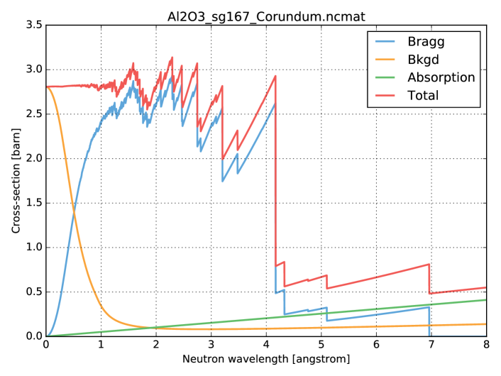
(a)

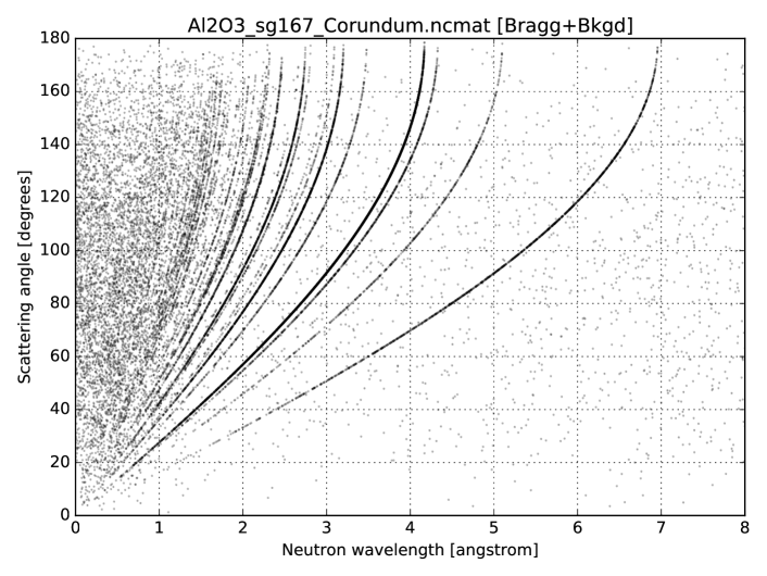
(b)

Figure 15: Plots produced by invoking ncrystal_inspectfile -a on a single configuration string (here "Al2O3_sg167_Corundum.ncmat").

By supplying the --dump flag, the graphical plotting will be replaced with a printout of loaded crystal information. For instance, the command:

⬇

ncrystal_inspectfile --dump "Cu2O_sg224_Cuprite.ncmat;dcutoff=1Aa"

results in the printout shown in Listing 3.

Listing 3: Printout produced by invoking ncrystal_inspectfile --dump on a single configuration string (here "Cu2O_sg224_Cuprite.ncmat;dcutoff=1Aa"). Refer to Table 2 for an explanation of the listed parameters.

⬇

---------------------------------------------------------

Space group number : 224

Lattice spacings [Aa] : 4.2685 4.2685 4.2685

Lattice angles [deg] : 90 90 90

Unit cell volume [Aa^3] : 77.7725

Atoms / unit cell : 6

---------------------------------------------------------

Atoms per unit cell (total 6):

2 O atoms [T_Debye=385.668K, MSD=0.0187741Aa^2]

4 Cu atoms [T_Debye=189.192K, MSD=0.0189719Aa^2]

---------------------------------------------------------

Atomic coordinates:

O 0 0 0

O 0.5 0.5 0.5

Cu 0.25 0.25 0.25

Cu 0.25 0.75 0.75

Cu 0.75 0.25 0.75

Cu 0.75 0.75 0.25

---------------------------------------------------------

Density : 6.11036 g/cm3

---------------------------------------------------------

Temperature : 293.15 kelvin

---------------------------------------------------------

Neutron cross-sections:

Absorption at 2200m/s : 2.52006 barn

Free scattering : 6.43997 barn

---------------------------------------------------------

HKL planes (d_lower = 1 Aa, d_upper = inf Aa):

H K L d_hkl[Aa] Multiplicity FSquared[barn]

0 1 -1 3.01829 12 1.2426

1 -1 -1 2.46442 8 8.42503

0 0 2 2.13425 6 3.14444

1 -2 -1 1.74261 24 1.056

0 2 -2 1.50914 12 13.0016

0 1 -3 1.34982 24 0.897427

1 -3 -1 1.287 24 6.06387

2 -2 -2 1.23221 8 2.25851

1 -3 -2 1.1408 48 0.762663

0 0 4 1.06713 6 9.36659

0 3 -3 1.0061 36 0.648137

---------------------------------------------------------

Figure 16 shows how specifying more than one configuration string at a time leads results in a plot comparing the resulting cross sections. Figure 16.a shows the total interaction cross section of thermal neutrons in a range of polycrystalline metals – which might for instance be considered for a support structure in some parts of a neutron instrument – and is the result of the command (all on one line):

⬇

ncrystal_inspectfile -a Al_sg225.ncmat Fe_sg229_Iron-alpha.ncmat

Cu_sg225.ncmat Ti_sg194.ncmat

Figure 16.b shows a similar plot, this time for a Beryllium powder at various temperatures, indicating the significance of beam filter cooling. It is the result of the command (all on one line):

⬇

ncrystal_inspectfile -a "Be_sg194.ncmat;temp=100K"

"Be_sg194.ncmat;temp=200K"

"Be_sg194.ncmat;temp=300K"

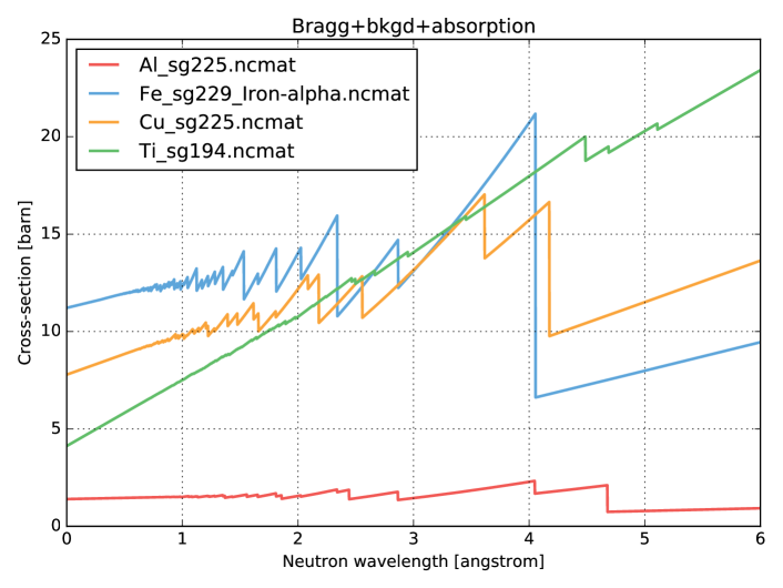
(a)

(b)

Figure 16: Plots produced by invoking ncrystal_inspectfile -a on multiple configuration strings. As a result, total interaction cross sections are shown for four different metals in (a), and for three beryllium powders at different temperatures in (b).

Finally, the command ncrystal_inspectfile --test can be used to validate a given installation of NCrystal. Although ncrystal_inspectfile already provides a useful set of functionality, it is expected that additional standard tools will be added in the future. In particular it would be useful with more options for plot creation and with utilities for assisting with the creation of configuration strings involving the alignment of single crystals, for instance to assist in the configuration of simulations involving neutron monochromators.

6.2 C++, C and Python bindings

Using the configuration strings presented in Section 5, the somewhat complicated C++ code in Listing 1 can be significantly simplified as shown in Listing 4: not only is it fewer lines, but the only material-specific code is the one defining the configuration string variable named cfg. It is thus straight-forward to create C++ applications or plugins which use NCrystal as a backend, but lets users provide the configuration strings in whichever frontend is relevant to the task at hand. The lingua franca of software is, however, the C programming language, and most modern programming languages contain some facility for interfacing with such code. In order to make NCrystal as widely useful as possible and able to support applications like McStas (cf. Section 6.4), a C interface is thus provided in the header file ncrystal.h, and the C equivalent of Listing 4 is shown in Listing 5. Although C does not support classes, an object-oriented paradigm is still achieved by providing the C code with handles instead of class instance pointers. Most C programmers should be familiar with such a scheme, as it is also encountered elsewhere, for instance in the form of file handles for file I/O. Although not quite as convenient as the C++ interface, C code using the created NCrystal handles essentially follow the same pattern as the equivalent C++ code. For instance, after retrieving the absn handle in Listing 5, it can be used in the following manner to provide a cross section in the variable xs, here for a $1.8\text{\,}\mathrm{\SIUnitSymbolAngstrom}\text{/}$ neutron incident along the $z$-axis:

⬇

double ekin = ncrystal_wl2ekin(1.8);

double dir[3] = {0.0, 0.0, 1.0};

double xs;

ncrystal_crosssection(absn, ekin, dir, &xs);

C does not support exceptions, so when using the C interface, any exceptions thrown internally in the NCrystal library due to errors will by default result in an appropriate error message being printed and the program terminated. For further details and a list of available functions, please refer to the header file ncrystal.h.

Listing 4: C++ code using a configuration string to create related NCrystal objects.

⬇

#include "NCrystal/NCrystal.hh"

namespace NC = NCrystal;//alias for convenience

int main() {

//Create objects based on a universal configuration string:

std::string cfg = "somefile.ncmat;temp=400K;dcutoff=0.5Aa;"

"bkgd=phonondebye:elastic";

const NC::Info * info = NC::createInfo(cfg);

const NC::Scatter * scat = NC::createScatter(cfg);

const NC::Absorption * absn = NC::createAbsorption(cfg);

// ...

// code here using info, scat and absn pointers

// ...

return 0;

}

Listing 5: C code using a configuration string to create related NCrystal object handles.

⬇

#include "NCrystal/ncrystal.h"

int main() {

/* Create objects based on a universal configuration string: */

const char * cfg = "somefile.ncmat;temp=400K;dcutoff=0.5Aa;"

"bkgd=phonondebye:elastic";

ncrystal_info_t info = ncrystal_create_info(cfg);

ncrystal_scatter_t scat = ncrystal_create_scatter(cfg);

ncrystal_absorption_t absn = ncrystal_create_absorption(cfg);

/* ... */

/* code here using info, scat and absn handles */

/* ... */

return 0;

}

Finally, it is possible to use NCrystal directly from Python [88], which mostly exists as a feature to support the usage of NCrystal for advanced scripting, analysis and plotting work. Python and C++ share concepts like classes and exceptions, and Python code using NCrystal thus ends up being similar and possibly even simpler than the corresponding C++ code, as can be seen in the Python equivalent of Listing 4, shown in Listing 6. Additionally, for efficiency and convenience, the Python interface supports vectorised access through Numpy [89] arrays. For a simple example using this, Listing 7 illustrates how to create a Matplotlib [90] plot of the scattering cross section as a function of neutron wavelengths between $0\text{\,}\mathrm{\SIUnitSymbolAngstrom}\text{/}$ and $10\text{\,}\mathrm{\SIUnitSymbolAngstrom}\text{/}$.

Listing 6: Python code using a configuration string to create related NCrystal objects.

⬇

import NCrystal as NC

cfg = """somefile.ncmat;temp=400K;dcutoff=0.5Aa;

bkgd=phonondebye:elastic"""

info = NC.createInfo(cfg)

scat = NC.createScatter(cfg)

absn = NC.createAbsorption(cfg)

# ...

# code here using info, scat and absn objects

# ...

Listing 7: Python code using the support in NCrystal for vectorised access through Numpy arrays, in order to plot scattering cross sections with Matplotlib.

⬇

#Create NCScatter object:

import NCrystal as NC

scat = NC.createScatter("<some-cfg-here>")

#Then plot via Numpy and Matplotlib:

import numpy

import matplotlib.pyplot as plt

wl = numpy.linspace( 0.0, 10.0, num=10000 )

xs = scat.crossSectionNonOriented( NC.wl2ekin( wl ) )

plt.plot(wl,xs)

plt.show()

As for any other Python module, documentation of the NCrystal module is built in and accessible via the help() function. Behind the scenes, the Python interface is implemented via the C interface using the ctypes Python module to call directly into the binary NCrystal library. Thus, no additional software dependencies are introduced by this interface – beyond naturally the Python interpreter itself.

6.3 Geant4 interface

Assuming Geant4 is configured to use a physics list which include the so-called HP (high precision) models for neutron physics, almost all comparisons between cross sections in Geant4 and NCrystal are qualitatively equivalent to the ones shown in Figure 17 for a magnesium powder. Starting around the $\text{\,}\mathrm{keV}\text{/}$ scale, Geant4 provides detailed modelling of higher energy effects such as those related to nuclear resonances. At lower energies, the cross section curves are, however, completely smooth and featureless due to the free-gas approximation used. NCrystal, on the other hand, provides detailed structure-dependent scattering physics at the sub-$\text{\,}\mathrm{eV}\text{/}$ scale – but has no capacity for modelling physics at the $\text{\,}\mathrm{keV}\text{/}$ scale. At intermediate energy scales, neither nuclear resonance physics or material structure-dependent physics introduce significant features, and there is an overlap in predictions between NCrystal and Geant4. For absorption processes, material structure is unimportant, and the predictions from NCrystal and Geant4 are in perfect agreement over the range covered by NCrystal, due to the validity of the simple $1/v$ scaling of such cross sections (cf. Section 2.2). However, unlike NCrystal, Geant4 provides detailed modelling of the secondary particles produced in absorption reactions. Consequently, the NCrystal plugin for Geant4 does not touch the absorption physics at all, instead focusing on replacing just the scattering physics for low energy neutrons. Presently this is done with a global hard-coded cross over point of $5\text{\,}\mathrm{eV}\text{/}$, but the exact transition model might be revisited in the future, since a few rare isotopes have nuclear resonances lower than this. As an example, the experimental data in Figure 14 indicates a resonance around $1.3\text{\,}\mathrm{eV}\text{/}$.

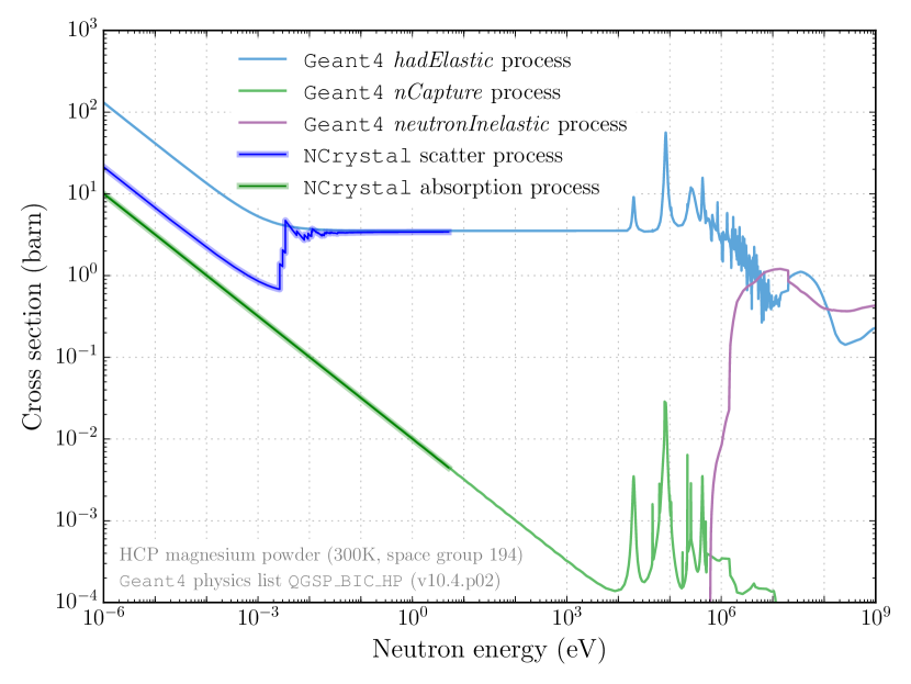
Figure 17: Neutron interaction cross sections in a magnesium powder, as predicted by Geant4 and NCrystal. At thermal neutron energies, absorption in Geant4 is handled by the Geant4 process named “nCapture”, while scattering (both elastic and inelastic) is handled by the process named “hadElastic”.

Geant4 user code requires very few changes in order to enable NCrystal modelling of scattering for low energy neutrons. First of all, the G4NCrystal.hh header file must be included. Next, materials for which it is desired to use NCrystal to provide scattering physics for thermal neutrons should be identified. Instances of G4Material for these materials must then be created by providing appropriate NCrystal configuration strings:

⬇

G4Material * mat =

G4NCrystal::createMaterial("Al_sg225.ncmat;temp=200K");

This creates a new G4Material, with relevant settings for standard parameters including atomic compositions, density and temperature, but additionally an NCrystal Scatter class instance is attached as a property. Created instances of G4Material must of course be subsequently inserted into the simulation geometry in the usual fashion for Geant4. For oriented materials, i.e. single crystals, it is the local orientation of the neutron with respect to the Geant4 volume which is passed to NCrystal. Thus, rotating volumes at the Geant4 level will also rotate the contained material structures, in line with what one might intuitively expect.

Finally, the Geant4 class instances representing physics processes must be modified, in order to ensure that the embedded Scatter instances are queried at the correct points during the simulations. This is presently done via a dynamic modification of the already loaded physics list, with code similar to:

⬇

runManager->Initialize();//Initialise G4RunManager

G4NCrystal::install();//Install NCrystal into G4 physics list

runManager->BeamOn(1000);//simulate 1000 events

This run-time modification of the physics list allows the usage of NCrystal with any existing physics list in which HP models have been activated. Although highly flexible, it is planned to also allow NCrystal to be used in a manner more customary in Geant4, hard-coding it into physics lists at compilation time. Additionally, it is intended that NCrystal should eventually be integrated into Geant4 releases, making the combined functionality available out of the box.

As an illustration, Figure 18 shows a visualisation of a Geant4 simulation in which the NCrystal plugin has been used to set up a single crystal monochromator. Although the simplistic example does not do justice to the capabilities of Geant4 to support arbitrarily complicated geometries, the novel potential for physics modelling with the setup is clear: the orientation of the crystal ensures that those neutrons in the incoming white beam possessing a compatible wavelength, will be reflected at exactly $135\text{\,}\mathrm{\SIUnitSymbolDegree}\text{/}$ in the $xy$-plane, which is the defining feature of a single crystal neutron monochromator. Multiple scattering and geometrical boundaries are naturally accounted for, and the reflected neutrons exhibit a characteristic “zig-zag” walk, and corresponding shifts in positions before leaving the crystal. Additionally featured are realistic processes such as both inelastic scatterings and absorption processes which results in the emission of energetic gamma particles, with a few subsequent Compton scatterings and pair conversions adding electrons and positrons into the mix.

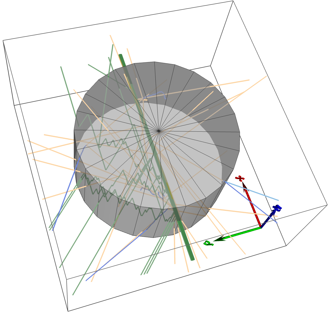
Figure 18: Simulation with Geant4 and NCrystal in which a polychromatic beam of neutrons (green), travelling along the $x$-axis, enters a cylindrical silicon crystal of radius $1\text{\,}\mathrm{mm}\text{/}$, oriented such that neutrons with $\lambda\approx$5.79\text{\,}\mathrm{\SIUnitSymbolAngstrom}\text{/}$$ will be scattered by $135\text{\,}\mathrm{\SIUnitSymbolDegree}\text{/}$ in the $xy$-plane by the lattice plane with Miller index $111$. Other particles appearing are gammas (yellow), electrons (blue), and positrons (light blue). Visualisation created with viewer from [20, 27] and used Geant4 physics list QGSP_BIC_HP (v10.0.p03).

Another example is shown in Figure 19, where it is illustrated how scattering of a monochromatic pencil beam of neutrons in an (untextured) polycrystalline sample changes qualitatively when NCrystal is enabled: instead of diffuse scattering due to the free-gas approximation, proper scattering into Debye-Scherrer cones by crystal planes is observed.

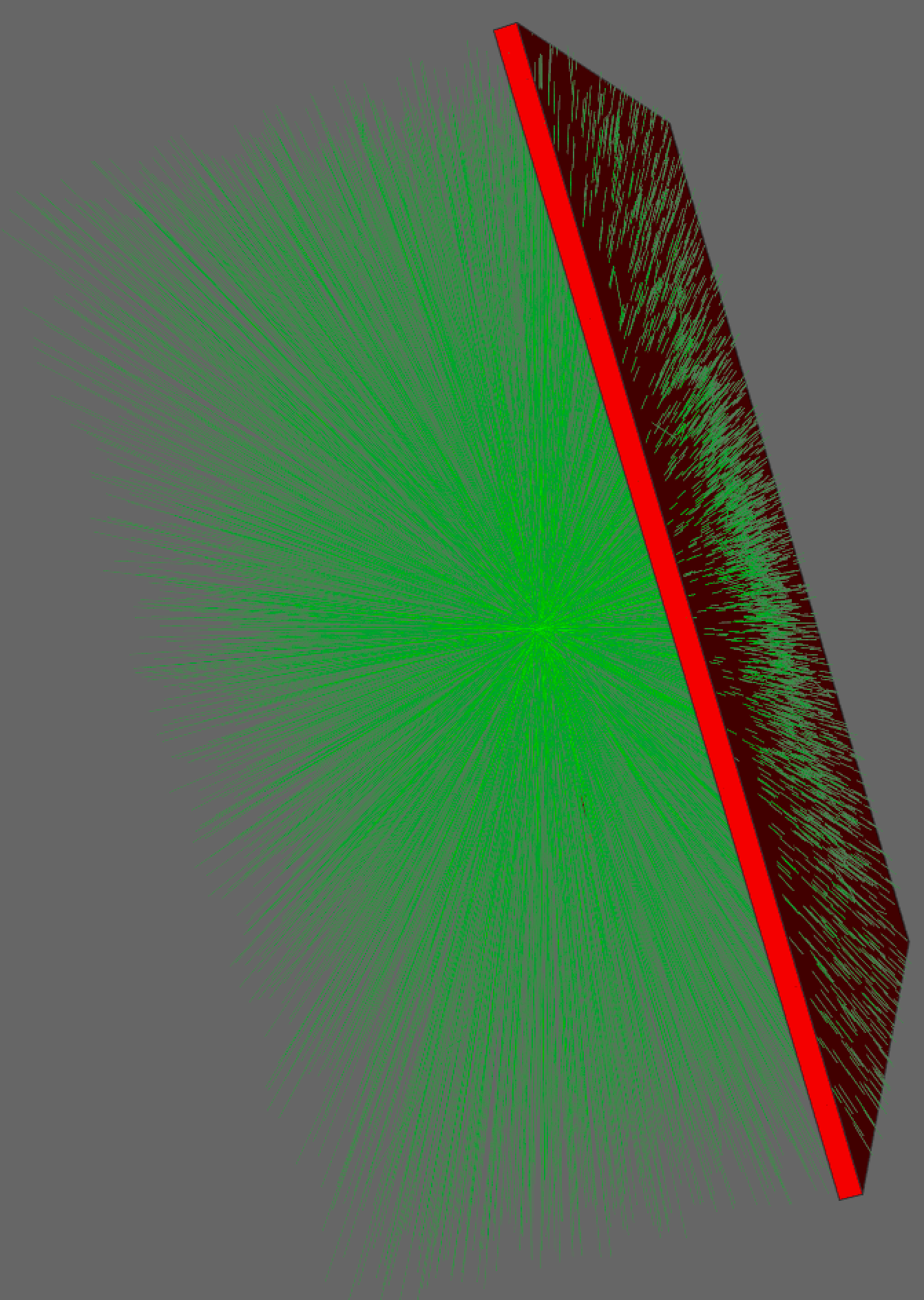
(a)

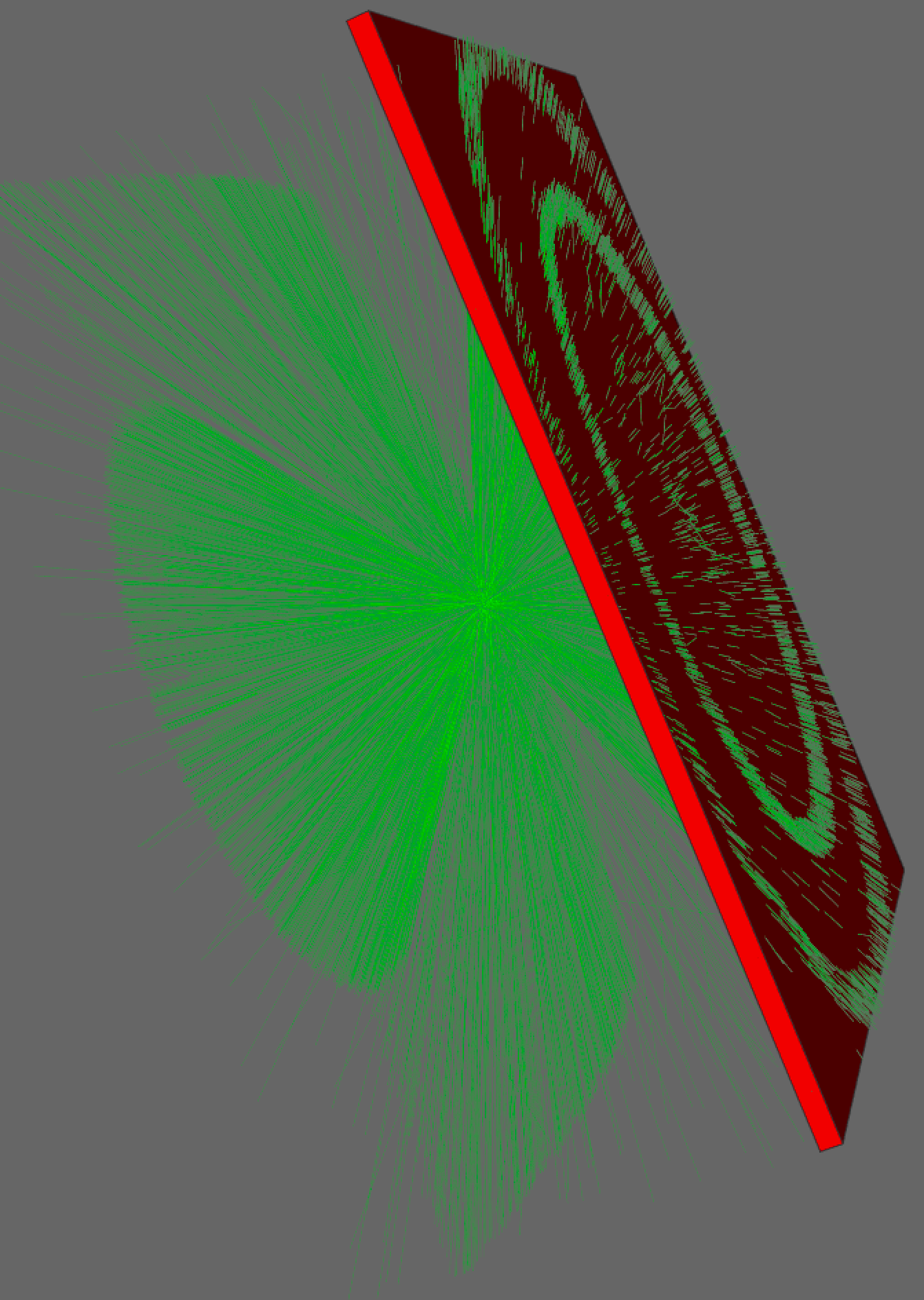
(b)

Figure 19: Simulation with Geant4 in which a monochromatic beam of neutrons (green), with wavelength $2.2\text{\,}\mathrm{\SIUnitSymbolAngstrom}\text{/}$, enters from the left and interacts with a small sample of polycrystalline aluminium. For clarity, other particle types such as gamma particles created as by-product of absorption events, are not shown. In (a) is shown the diffuse scattering resulting from the free-gas approximation when using Geant4 out of the box with physics list QGSP_BIC_HP (v10.0.p03). In (b) is shown the more realistic scattering into Debye-Scherrer cones, resulting from using NCrystal to provide polycrystalline structure to the sample. Visualisation created with viewer from [20, 27].

6.4 McStas interface

In McStas simulations, thermal neutrons are passed through an ordered list of components configured by users in a so-called instrument file. Components typically represent actual in-beam elements found at the modelled neutron instrument such as: source, optical guides, choppers, filters, monochromators, analysers, samples, or detectors. Each component is responsible for modelling both geometrical and physics effects, and in addition to scattering, absorption physics can be implemented either by trajectory termination or intensity reduction.

The NCrystal plugin for McStas is provided as a component with the name NCrystal_sample, but it can be used to model a variety of elements in addition to samples, including filters, monochromators, and analysers. For now, it accepts a single configuration string for NCrystal and implements a material in either a spherical, cylindrical, or box-shaped geometry. By default it implements absorption via intensity reduction and allows for multiple scattering interactions, but both of these aspects are configurable. Full usage instructions are available via the usual mcdoc documentation system of McStas. The component is implemented by using the C bindings for NCrystal.

Listing 8 shows an example of a McStas instrument file in which neutrons from a simplistic source model are reflected onto a cylindrical NCrystal sample of yttrium-oxide powder by a box-shaped NCrystal copper monochromator aligned to reflect on the $hkl=002$ plane. Finally, neutrons reflected by the powder sample are recorded by a “banana-shaped” detector array. The beam-monochromator setup is tuned to provide a $90\text{\,}\mathrm{\SIUnitSymbolDegree}\text{/}$ scatter angle ($\theta_{\text{B}}=$45\text{\,}\mathrm{\SIUnitSymbolDegree}\text{/}$$), when the incident neutron wavelength fulfils the Bragg condition $\lambda=2d_{002}\sin\theta_{\text{B}}$, evaluating to $2.556\,16\text{\,}\mathrm{\SIUnitSymbolAngstrom}\text{/}$ when using a value $d_{002}=$1.807\,48\text{\,}\mathrm{\SIUnitSymbolAngstrom}\text{/}$$ – which could have been extracted programmatically but for simplicity it was in this case determined by the user via the interactive tool described in Section 6.1. Figure 20 shows a 3D visualisation of the resulting simulation using McStas 2.4.1, while Figure 21 shows the corresponding diffraction pattern observed in the modelled detector array.

Listing 8: Simple McStas instrument file using NCrystal for monochromator and sample.

⬇

DEFINE INSTRUMENT example()

TRACE

COMPONENT origin = Progress_bar()

AT (0,0,0) RELATIVE ABSOLUTE

COMPONENT source = Source_div

( lambda0 = 2.55616, dlambda = 0.01, xwidth = 0.001,

yheight = 0.001, focus_aw = 0.4, focus_ah = 0.4 )

AT (0,0,0.3) RELATIVE origin

COMPONENT arm1 = Arm()

AT (0,0,0.5) RELATIVE source ROTATED (0,45,0) RELATIVE source

COMPONENT monochromator = NCrystal_sample

( xwidth = 0.05, yheight = 0.05, zdepth = 0.003,

cfg = "Cu_sg225.ncmat;mos=0.3deg;bkgd=0"

";dir1=@crys_hkl:0,0,2@lab:0,0,1"

";dir2=@crys_hkl:1,0,0@lab:0,1,0" )

AT (0,0,0) RELATIVE arm1

COMPONENT arm2 = Arm()

AT (0,0,0) RELATIVE arm1 ROTATED (0,-90,0) RELATIVE source

COMPONENT powder_sample = NCrystal_sample

( yheight = 0.03, radius = 0.01,

cfg = "Y2O3_sg206_Yttrium_Oxide.ncmat;packfact=0.8" )

AT (0,0,0.4) RELATIVE arm2

COMPONENT detectors = Monitor_nD

( options = "banana, angle limits=[10 170], bins=500",

radius = 0.2, yheight = 0.2 )

AT (0,0,0) RELATIVE powder_sample

END

Figure 20: McStas visualisation of the simulation resulting from the instrument file shown in Listing 8. Neutrons impinge on the monochromator box (light-blue) from the right, and are reflected in the horizontal plane towards the cylindrical powder sample (also light-blue). The detector array (yellow) captures parts of the Debye-Scherrer cones created by reflections in the sample.

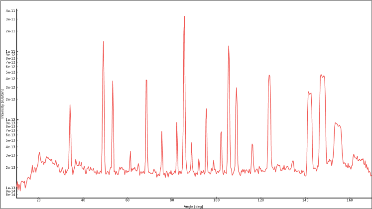
Figure 21: McStas diffraction pattern resulting from a simulation of ${10}^{7}$ source neutrons using the instrument file shown in Listing 8. The shown intensity in each of the 500 bins corresponds to a source flux of $1\text{\,}\mathrm{n}\mathrm{e}\mathrm{u}\mathrm{t}\mathrm{r}\mathrm{o}\mathrm{n}\mathrm{/}\mathrm{s}\mathrm{/}\mathrm{{}^{2}}\mathrm{c}\mathrm{m}\mathrm{/}\mathrm{sr}\mathrm{/}\mathrm{\SIUnitSymbolAngstrom}$.

In addition to benefiting from future improvements to the NCrystal library, it is foreseen that the NCrystal_sample McStas component itself might also be further enhanced at a later state. In particular, it would be desirable to implement variance reduction techniques, at least in terms of making it possible to focus outgoing neutrons towards the next down-stream component. It is also likely that use-cases for more advanced geometrical layouts will arise, and the code has consequently been structured in a way which makes it straight-forward to add such features.

7 Outlook

The presented toolkit for thermal neutron transport is arguably unique in its attention to interfaces and capability for integration into various technical contexts and is already in version 1.0.0 very capable in terms of modelling of interactions in single crystals and crystal powders, and has already been used to enable a range of interesting studies (e.g. [20, 53, 91, 92, 93, 94, 95, 96, 97]).

Nonetheless, work has already begun on several improvements to both physics models and the framework itself. Firstly, as mentioned in Section 2.4, the capabilities for modelling of inelastic and incoherent scattering should see significant enhancements – with the possibility of supporting liquids or polymers to some extent. These models, and those implementing Bragg diffraction, will be described in detail in future dedicated publications.

Next, it is the plan to carry out framework extensions and refactorisations which will allow NCrystal to support enhanced material realism, by making the exact composition of materials and crystals more customisable. Once implemented, it should on one hand become possible to support multi-phase materials – needed for realistic multi-phase metal alloys or crystal powders suspended in liquids – and on the other hand the composition of each phase should become more flexible as well, allowing for enriched materials or chemical disorder. That would enable modelling of crystals in which some sites are not fully occupied in all cells – or occasionally occupied with elements playing the role of contaminants or dopants.

Several more technical developments are envisioned as well: planned interface extensions will enable better support of multi-threaded applications (such as ANTS2 or multi-threaded builds of Geant4), and several use-cases have been identified where it would be advantageous to be able to initialise crystal data directly from process memory rather than needing on-disk files. In the longer run, once all relevant platforms and applications support it, it is also planned to drop the support for the C++98 standard, in order to better benefit from modern C++ features and better cross platform support introduced in C++11 and beyond.

Beyond that, the future directions will depend on resources and community interest. At the very least the library of data files and the list of Monte Carlo applications with NCrystal support are both expected to expand. But given sufficient interest and contributions new ambitious physics models could be added, ranging from treatment of texture, bent crystals and new anisotropic mosaicity models to better facilities for dealing with nuclear resonances or branching into new areas like magnetic spin-dependent interactions or support of X-ray physics. Input, feedback, ideas or contributions are gratefully received via the NCrystal website [34].

References

References

- Metropolis [1987] N. Metropolis, Los Alamos Science 15 (1987) 125–130.
- Waters et al. [2007] L. S. Waters, et al., AIP Conf. Proc. 896 (2007) 81–90. doi:10.1063/1.2720459.
- X-5 Monte Carlo Team [2003] X-5 Monte Carlo Team, MCNP - A General N-Particle Transport Code, Version 5, Technical Report, Los Alamos National Laboratory, 2003. Volume II: User’s Guide, LA-CP-03-0245.
- Goorley et al. [2013] J. Goorley, et al., Initial MCNP6 Release Overview - MCNP6 version 1.0, Technical Report LA-UR-13-22934, Los Alamos National Laboratory, 2013.
- Agostinelli et al. [2003] S. Agostinelli, et al., Nucl. Instrum. Meth. A506 (2003) 250–303. doi:10.1016/S0168-9002(03)01368-8.
- Allison et al. [2006] J. Allison, et al., IEEE Trans. Nucl. Sci. 53 (2006) 270. doi:10.1109/TNS.2006.869826.
- Allison et al. [2016] J. Allison, et al., Nucl. Instrum. Meth. A835 (2016) 186 – 225. doi:10.1016/j.nima.2016.06.125.
- Böhlen et al. [2014] T. T. Böhlen, et al., Nucl. Data Sheets 120 (2014) 211 – 214. doi:10.1016/j.nds.2014.07.049.
- Sato et al. [2018] T. Sato, et al., J. Nucl. Sci. Technol. 55 (2018) 684–690. doi:10.1080/00223131.2017.1419890.
- Leppänen et al. [2015] J. Leppänen, et al., Ann. Nucl. Energy 82 (2015) 142 – 150. doi:10.1016/j.anucene.2014.08.024.
- Romano et al. [2015] P. K. Romano, et al., Ann. Nucl. Energy 82 (2015) 90 – 97. doi:10.1016/j.anucene.2014.07.048.
- Lefmann and Nielsen [1999] K. Lefmann, K. Nielsen, Neutron News 10 (1999) 20–23. doi:10.1080/10448639908233684.
- Willendrup et al. [2004] P. Willendrup, et al., Physica B: Condensed Matter 350 (2004) E735 – E737. doi:10.1016/j.physb.2004.03.193.
- Zsigmond et al. [2002] G. Zsigmond, et al., Neutron News 13 (2002) 11–14. doi:10.1080/10448630208218488.
- Lieutenant et al. [2004] K. Lieutenant, et al., Proc. SPIE 5536 (2004). doi:10.1117/12.562814.
- Šaroun and Kulda [1997] J. Šaroun, J. Kulda, Physica B: Condensed Matter 234-236 (1997) 1102 – 1104. doi:10.1016/S0921-4526(97)00037-9.
- Seeger et al. [2002] P. A. Seeger, et al., Neutron News 13 (2002) 20–23. doi:10.1080/10448630208218490.
- Brown et al. [2018] D. Brown, et al., Nucl. Data Sheets 148 (2018) 1 – 142. doi:10.1016/j.nds.2018.02.001.
- Damián et al. [2014] J. M. Damián, et al., Ann. Nucl. Energy 65 (2014) 280 – 289. doi:10.1016/j.anucene.2013.11.014.
- Kanaki et al. [2018] K. Kanaki, et al., Physica B: Condensed Matter 551 (2018) 386 – 389. doi:10.1016/j.physb.2018.03.025.
- Cherkashyna et al. [2014] N. Cherkashyna, et al., J. Phys: Conf. Ser. 528 (2014) 012013. doi:10.1088/1742-6596/528/1/012013.
- Xu et al. [2008] X. G. Xu, et al., Phys. Med. Biol. 53 (2008) R193. doi:10.1088/0031-9155/53/13/R01.
- Newhauser and Durante [2011] W. D. Newhauser, M. Durante, Nature Reviews Cancer 11 (2011) 438–448. doi:10.1038/nrc3069.
- Garoby et al. [2018] R. Garoby, et al., Phys. Scripta 93 (2018) 014001. doi:10.1088/1402-4896/aa9bff.
- Peggs et al. [2012] S. Peggs, et al., ESS Conceptual Design Report, ESS 2012-001, 2012.
- Peggs et al. [2013] S. Peggs, et al., ESS Technical Design Report, ESS 2013-001, 2013.
- Kittelmann et al. [2014] T. Kittelmann, et al., J. Phys: Conf. Ser. 513 (2014) 022017. doi:10.1088/1742-6596/513/2/022017.
- Kropff and Granada [1977] F. Kropff, J. R. Granada, CRIPO: A Fast Computer Code for the evaluation of in Polycrystalline materials, 1977. Instituto Balseiro, Bariloche, Argentina (Unpublished report).
- MacFarlane et al. [2012] R. E. MacFarlane, et al., The NJOY Nuclear Data Processing System, Version 2012, Technical Report LA-UR-12-27079, Los Alamos National Laboratory, 2012.
- Boin [2012] M. Boin, J. Appl. Cryst. 45 (2012) 603–607. doi:10.1107/S0021889812016056.
- Kittelmann and Boin [2015] T. Kittelmann, M. Boin, Comput. Phys. Commun. 189 (2015) 114 – 118. doi:10.1016/j.cpc.2014.11.009.
- The Apache Software Foundation [2004] The Apache Software Foundation, Apache License, Version 2.0, January 2004. URL: http://www.apache.org/licenses/LICENSE-2.0.html.
- Martin and Hoffman [2015] K. Martin, B. Hoffman, Mastering CMake: A Cross-Platform Build System, Kitware Inc, 2015.
- Cai and Kittelmann [2018] X.-X. Cai, T. Kittelmann, Website of NCrystal: a library for thermal neutron transport, 2018. URL: https://mctools.github.io/ncrystal/. doi:10.5281/zenodo.853186.
- Sands [1993] D. Sands, Introduction to Crystallography, Dover Books on Chemistry Series, Dover Publications, 1993. Orig. publ.: W.A. Benjamin, 1969 (corr. 1975).
- Kittel [2004] C. Kittel, Introduction to Solid State Physics, 8th ed., Wiley, 2004.
- Waseda et al. [2011] Y. Waseda, et al., X-Ray Diffraction Crystallography: Introduction, Examples and Solved Problems, Springer, 2011.
- Hahn and of Crystallography [2002] T. Hahn, I. U. of Crystallography, International Tables for Crystallography, Space-Group Symmetry, International Tables for Crystallography, Wiley, 2002.
- Wyckoff [1922] R. W. G. Wyckoff, The Analytical Expression of the Results of the Theory of Space-groups, Carnegie Institution of Washington, 1922.
- Squires [2012] G. L. Squires, Introduction to the Theory of Thermal Neutron Scattering, 3 ed., Cambridge University Press, 2012. doi:10.1017/CBO9781139107808.
- Schober [2014] H. Schober, J. Neutron Res. 17 (2014) 109–357. doi:10.3233/JNR-140016.
- Marshall and Lovesey [1971] W. Marshall, S. W. Lovesey, Theory of thermal neutron scattering: the use of neutrons for the investigation of condensed matter, Clarendon Press Oxford, 1971.
- Sears [1986] V. F. Sears, Phys. Rep. 141 (1986) 281 – 317. doi:10.1016/0370-1573(86)90129-8.
- Fermi [1936] E. Fermi, La Ricerca Scientifica 7 (1936) 13–52.
- van Sluijs et al. [2015] R. van Sluijs, et al., J Radioanal. Nucl. Ch. 306 (2015). doi:10.1007/s10967-015-4134-1.
- Sears [1984] V. Sears, Thermal-neutron scattering lengths and cross sections for condensed-matter research, Technical Report AECL–8490, Chalk River Nuclear Laboratories, Canada, 1984.
- Breit and Wigner [1936] G. Breit, E. Wigner, Phys. Rev. 49 (1936) 519–531. doi:10.1103/PhysRev.49.519.
- Bethe [1935] H. A. Bethe, Phys. Rev. 47 (1935) 747–759. doi:10.1103/PhysRev.47.747.
- Freund [1983] A. Freund, Nucl. Instr. Meth. 213 (1983) 495–501. doi:10.1016/0167-5087(83)90447-7.
- Cassels [1950] J. Cassels, Prog. Nucl. Phys. 1 (1950) 185 – 215.
- Binder [1970] K. Binder, Phys. Stat. Sol. 41 (1970) 767–779. doi:10.1002/pssb.19700410233.
- Adib and Fathalla [2007] M. Adib, M. Fathalla, Egyptian Nuclear Physics Association (ENPA), Egyptian Atomic Energy Authority (EAEA), 6th Conference on Nuclear and Particle Physics, Luxor (Egypt) 642 (2007) 39–54.
- Cai et al. [2019] X.-X. Cai, et al., J. Comput. Phys. 380 (2019) 400 – 407. doi:10.1016/j.jcp.2018.11.043.
- Sjölander [1958] A. Sjölander, Arkiv För fysik 14 (1958) 315–371.
- Placzek [1952] G. Placzek, Phys. Rev. 86 (1952) 377–388. doi:10.1103/PhysRev.86.377.
- Debye [1912] P. Debye, Annalen der Physik 344 (1912) 789–839. doi:10.1002/andp.19123441404.
- Glauber [1955] R. J. Glauber, Phys. Rev. 98 (1955) 1692. doi:10.1103/PhysRev.98.1692.
- Peng et al. [1996] L.-M. Peng, et al., Acta Crystallogr. A 52 (1996) 456–470. doi:10.1107/S010876739600089X.
- Wang et al. [2013] B.-T. Wang, et al., Phys. Rev. B 88 (2013) 104107. doi:10.1103/PhysRevB.88.104107.
- Blackman and Vigna [2018] D. Blackman, S. Vigna, Scrambled linear pseudorandom number generators, 2018. URL: http://arxiv.org/abs/1805.01407.
- Hall et al. [1991] S. R. Hall, et al., Acta Crystallogr. A 47 (1991) 655–685. doi:10.1107/S010876739101067X.
- Gražulis et al. [2009] S. Gražulis, et al., J. Appl. Cryst. 42 (2009) 726–729. doi:10.1107/S0021889809016690.
- Downs and Hall-Wallace [2003] R. T. Downs, M. Hall-Wallace, Am. Mineral. 88 (2003) 247.
- Larsen et al. [2017] A. H. Larsen, et al., Journal of Physics: Condensed Matter 29 (2017) 273002. doi:10.1088/1361-648X/aa680e.
- Wyckoff [1963] R. Wyckoff, Crystal Structures, volume 1, Wiley, 1963.
- Kirfel and Eichhorn [1990] A. Kirfel, K. Eichhorn, Acta Crystallogr. A 46 (1990) 271–284. doi:10.1107/S0108767389012596.
- Ghalsasi and Ghalsasi [2011] P. Ghalsasi, P. S. Ghalsasi, Inorg. Chem. 50 (2011) 86–89. doi:10.1021/ic101248g.
- Trucano and Chen [1975] P. Trucano, R. Chen, Nature 258 (1975) 136 – 137. doi:10.1038/258136a0.
- Antao and Hassan [2009] S. M. Antao, I. Hassan, Can. Mineral. 47 (2009) 1245. doi:10.3749/canmin.47.5.1245.
- Hazen [1976] R. M. Hazen, Am. Mineral. 61 (1976) 266 – 271.
- Antao et al. [2008] S. M. Antao, et al., Can. Mineral. 46 (2008) 1501. doi:10.3749/canmin.46.5.1501.
- Gustafsson et al. [2001] T. Gustafsson, et al., Acta Crystallogr. C 57 (2001) 668–669. doi:10.1107/S0108270101005352.
- Park et al. [2011] W. B. Park, et al., J. Mater. Chem. 21 (2011) 5780–5785. doi:10.1039/C0JM03538F.
- Jericha and Hainbuchner [2001] E. Jericha, M. Hainbuchner, Neutron Scattering Lengths, 2001. URL: http://www.ati.ac.at/~neutropt/scattering/table.html.
- Rauch and Waschkowski [2000] H. Rauch, W. Waschkowski, 6 Neutron scattering lengths, Springer, Berlin, Heidelberg, 2000, pp. 1–29. doi:10.1007/10499706_6.
- Koester et al. [1991] L. Koester, et al., Atom. Data Nucl. Data 49 (1991) 65 – 120. doi:10.1016/0092-640X(91)90012-S.
- Boin et al. [2011] M. Boin, et al., J. Appl. Cryst. 44 (2011) 1040–1046. doi:10.1107/S0021889811025970.
- Boin et al. [2012] M. Boin, et al., J. Phys: Conf. Ser. 340 (2012) 012022. doi:10.1088/1742-6596/340/1/012022.
- Grosse-Kunstleve [1998] R. W. Grosse-Kunstleve, SgInfo, a Comprehensive Collection of ANSI C Routines for the Handling of Space Groups, http://cci.lbl.gov/sginfo/, 1998.
- Vogel [2000] S. Vogel, A Rietveld-Approach for the Analysis of Neutron Time-Of-Flight Transmission Data, Ph.D. thesis, Christian-Albrecht-Univ. Kiel, 2000.
- Yvon et al. [1977] K. Yvon, et al., J. Appl. Cryst. 10 (1977) 73–74. doi:10.1107/S0021889877012898.
- Siegrist [1997] T. Siegrist, J. Appl. Cryst. 30 (1997) 418–419. doi:10.1107/S0021889897003026.
- Farhi et al. [2014] E. Farhi, et al., J. Neutron Res. 17 (2014) 5–18. doi:10.3233/JNR-130001.
- Toby and Von Dreele [2013] B. H. Toby, R. B. Von Dreele, J. Appl. Cryst. 46 (2013) 544–549. doi:10.1107/S0021889813003531.
- Rodríguez-Carvajal [1993] J. Rodríguez-Carvajal, Physica B: Condensed Matter 192 (1993) 55 – 69. doi:10.1016/0921-4526(93)90108-I.
- Otuka et al. [2014] N. Otuka, et al., Nucl. Data Sheets 120 (2014) 272 – 276. doi:10.1016/j.nds.2014.07.065.
- Morozov et al. [2016] A. Morozov, et al., J. Instrum. 11 (2016) P04022. doi:10.1088/1748-0221/11/04/P04022.
- van Rossum and Drake [2011] G. van Rossum, F. L. Drake, The Python Language Reference Manual, Network Theory Ltd., 2011.
- Oliphant [06 ] T. Oliphant, NumPy: A guide to NumPy, Trelgol Publishing, 2006–. URL: http://www.numpy.org/.
- Hunter [2007] J. D. Hunter, Comput. Sci. Eng. 9 (2007) 90–95. doi:10.1109/MCSE.2007.55.
- Santoro et al. [2015] V. Santoro, et al., J. Neutron Res. 18 (2015) 135–144. doi:10.3233/JNR-160034.
- Dian et al. [2017] E. Dian, et al., in: 2017 IEEE Nuclear Science Symposium and Medical Imaging Conference (NSS/MIC), pp. 1–3. doi:10.1109/NSSMIC.2017.8532930.
- Messi et al. [2017] F. Messi, et al., The neutron tagging facility at Lund University, 2017. URL: http://arxiv.org/abs/1711.10286.
- Kanaki et al. [2018] K. Kanaki, et al., J. Instrum. 13 (2018) P07016. doi:10.1088/1748-0221/13/07/P07016.
- Mauri et al. [2018] G. Mauri, et al., J. Instrum. 13 (2018) P03004. doi:10.1088/1748-0221/13/03/P03004.
- Galgóczi et al. [2018] G. Galgóczi, et al., J. Instrum. 13 (2018) P12031. doi:10.1088/1748-0221/13/12/P12031.
- Dian et al. [2019] E. Dian, et al., J. Instrum. 14 (2019) P01021. doi:10.1088/1748-0221/14/01/p01021.