Modeling the large-scale power deficit
with smooth and discontinuous primordial spectra

Abstract

We study primordial power spectra with a large-scale power deficit and their effect on the standard $\Lambda$CDM cosmology. The standard power-law spectrum is subject to long-wavelength modifications described by some new parameters, resulting in corrections to the anisotropies in the cosmic microwave background. The new parameters are fitted to different datasets: Planck 2015 data for temperature and for both temperature and polarization, the low-redshift determination of $H_{0}$, and distances derived from baryonic acoustic oscillations. We discuss the statistical significance of the modified spectra, from both frequentist and Bayesian perspectives. Our analysis suggests motivations for considering models that break scalar-tensor consistency, or models with negligible power in the far super-Hubble limit. We present what appears to be substantial evidence, according to the Jeffreys’ scale, for a new length scale around 2200 Mpc ($k^{-1}\sim 350$ Mpc) above which the primordial (scalar) power spectrum is sharply reduced by about 20%.

I Introduction

Cosmological data is now accumulating at such a rate that the phrase ‘precision cosmology’ is often used to describe our current understanding of the primordial universe Peter and Uzan (2013). As is well known, the largest scales show features whose significance is unclear and which remain controversial Schwarz et al. (2016). In particular, the existence or otherwise of a large-scale power deficit remains an open question. A natural way to address this, explored in the present paper, is to postulate that the primordial power spectrum is suppressed at large scales by some as-yet-unknown physical mechanism Chluba et al. (2015). Assuming a phenomenological parametrization of the modification, which we shall from now on refer to as a deficit function, we may then analyze the available data and evaluate the statistical significance of any proposed modified spectrum.

A previous similar analysis of the Planck data from the cosmic microwave background (CMB) was carried out by the Planck team Planck Collaboration et al. (2014a); Ade et al. (2016), specifically for their temperature and polarization data. They considered, among other possibilities, two modifications of the primordial power spectrum with suppressed power on large scales modeled by two extra parameters. They concluded that “neither of these two models with two extra parameters is preferred over the base $\Lambda$CDM model”. In a more recent analysis Planck Collaboration et al. (2018), other models (and features) based on inflationary scenarios were also considered, for which they again found no supporting evidence. Even so, observations and statistical tests of this deficit have a much longer history. The first hint of a large-scale power deficit was already present in the first detection of the CMB anisotropies by the COBE DMR experiment (see the four-year results summary in Ref.  Bennett et al. (1996)). This feature was later observed by WMAP Bennett et al. (2003), and in Ref. Spergel et al. (2003) they introduced the statistic $S_{1/2}$ to measure the lack of power at large angular scales ($>60{}^{\circ}$) for the angular two-point correlation function and obtained a moderate-to-strong significance for the low power (only $0.15\%$ of the simulations had the same low power). Following the WMAP result, several different approaches were proposed to model and/or to test for low power at large scales (see for example Contaldi et al. (2003); Bridle et al. (2003); Efstathiou (2003a, b); Kawasaki and Takahashi (2003); de Oliveira-Costa et al. (2004); Martin and Ringeval (2004)). These included spatially curved models Park and Ratra (2018), modified inflation, and purely phenomenological modifications of the primordial power spectrum (PPS), among others. Besides the low power at large angular scales, other so-called anomalies have also been considered (see for example Ref.  Muir et al. (2018) for a summary of these anomalies and tests of their statistical significance). While statistical analysis of “anomalies” can shed light on their significance, these a posteriori methods tend to overestimate the significance. A statistical test including the whole fit provides a clearer picture of the significance of the proposed anomaly (see for example Refs.  Contaldi et al. (2003); Bennett et al. (2011)).

The purpose of this paper is to revisit the Planck team’s conclusions by considering a wider set of possible deficit functions together with a wider set of cosmological data – specifically including the low-redshift determination of $H_{0}$ Riess et al. (2016) (leading to $H_{0}=73.24\pm 1.74\,\hbox{km}\cdot\hbox{s}^{-1}\cdot\hbox{Mpc}^{-1}$ which is in tension with the Planck result $H^{\mathrm{Planck}}_{0}\sim 67.3\,\hbox{km}\cdot\hbox{s}^{-1}\cdot\hbox{Mpc}^{-1}$) and the distances derived from baryonic acoustic oscillations (BAO). In particular we extend the exponential cutoff model used in Refs. Planck Collaboration et al. (2014a); Ade et al. (2016) by including a maximum-deficit parameter, which leads us to new results as we will see below.

In our original motivating model for a physical large-scale power deficit, the primordial perturbations are produced in a preinflationary radiation-dominated phase Wang and Ng (2008) that is in a state of “quantum nonequilibrium” Colin and Valentini (2015, 2016, 2013) (resulting in violations of the usual Born rule, a possibility that is allowed in the de Broglie-Bohm pilot-wave formulation of quantum mechanics Valentini (2010)). Dynamical relaxation to quantum equilibrium (that is, to the Born rule) is found to be suppressed at very large wavelengths, thereby naturally producing a dip in the primordial power spectrum at large scales. If we add the simplifying assumption that the spectrum is unchanged by the transition from preinflation to inflation, we obtain a three-parameter modification of the CMB spectrum (noting that quantum relaxation may be shown to not take place during inflation itself Valentini (2010)). In this paper we extend the modification to four parameters in order to be able to compare with the cases studied by the Planck team.

We have found that Planck data (temperature only, with no polarization) combined with the low-redshift determination of $H_{0}$ and the distances derived from baryonic oscillations are able to constrain two of the new parameters fairly well, yielding a moderate improvement at the $2-3\sigma$ level in favor of our quantum relaxation model (in particular for the combination of temperature data with $H_{0}$ alone). However, the significance of the fits tends to decrease when polarization data are added. We then seem driven to the conclusion that our starting point for a modified power spectrum yields statistically inconclusive results. Alternatively, however, peculiarities of the fit when polarization data are added suggest that a better fit might be obtained in a model that allows for a breaking of scalar-tensor consistency. Our analysis suggests a motivation for considering such models, which arise naturally in quantum relaxation scenarios. Our results also suggest a motivation for considering models with negligible power in the far super-Hubble limit.

Additionally, in the course of our analysis we found that the fitting process led naturally to a preference for an extreme case of our (scalar) deficit function. The best fit seems to be obtained with a simple two-parameter sharp decrease in the power spectrum, with a statistical significance ranging from substantial to strong (according to Jeffreys’ scale given in Ref. (Jeffreys, 1998, Appendix B)). We find a good account of the data with a sudden dip of about 20% at a characteristic scale of around $2\pi k^{-1}\approx 2200~{}\mathrm{Mpc}~{}(k^{-1}\approx 350~{}\mathrm{Mpc})$; a first analysis leading to a similar effect was discussed in Ref. Hazra et al. (2013) for the Planck 2013 data. Whether or not this provides a new physically relevant scale in other areas of cosmology is left for future investigation.

In Sec. II we present our cosmological model and our parametrizations of the modified power spectrum. In Sec. III we describe the methodology for our statistical data analysis. Our numerical approach is summarized in Sec. IV. Our results are presented and discussed in detail in Sec. V. The significance and properties of the sudden jump deficit function are discussed in Section V.3. A possible breaking of scalar-tensor consistency is briefly addressed in Sec. V.4. The implications of our results for future work on quantum relaxation scenarios are summarized in Sec. VI. Our conclusions are drawn in Sec. VII. These are followed by two appendices. Appendix A discusses the cosmology library used in our numerical analysis, while Appendix B provides more details of our data analysis.

II Cosmological Model

Even though the CMB anisotropies depend strongly on the primordial power spectrum, they also depend on other aspects of the cosmological model which are unrelated to the origin of the primordial perturbations. For this reason, we start by specifying the complete cosmological model that we use to calculate the CMB anisotropies theoretically.

II.1 Deficit functions

In what follows we do not adopt a particular inflationary model (or any reasonable alternative one might consider Peter and Pinto-Neto (2008); Battefeld and Peter (2015); Brandenberger and Peter (2017); Bacalhau et al. (2018)) but only a simple power-law model of the fiducial power spectrum as best fitted by all currently available data. We also assume, again in accordance with known data, that only the adiabatic mode is present. We do not consider any contribution from gravitational waves. In such a framework, all the information about the primordial perturbations is contained in the fiducial power spectrum (with “_plaw” denoting “power-law”)

$$\mathcal{P}_{\mathrm{F}}(k)=\mathcal{P}_{\mathrm{plaw}}(k)\equiv\mathcal{A}_{\mathrm{s}}\left(\frac{k}{k_{\star}}\right)^{n_{\mathrm{s}}-1},$$ (1)

where $k_{\star}$ is the pivotal mode chosen (following the Planck analysis) to be $k_{\star}=0.05\,\mathrm{Mpc}^{-1}$, $\mathcal{A}_{\mathrm{s}}$ is the amplitude of the adiabatic mode measured at $k_{\star}$, and $n_{\mathrm{s}}$ is the spectral index. The modified power spectrum may then be described by a deficit function $\xi(k)$, or alternatively $\chi(k)\equiv 1-\xi(k)$, defined by

$$\mathcal{P}(k)=\xi(k)\mathcal{P}_{\mathrm{F}}(k)=\left[1-\chi(k)\right]\mathcal{P}_{\mathrm{F}}(k).$$ (2)

Here $\mathcal{P}(k)$ is the effective (to be estimated) power spectrum and $\lim_{k\gg k_{\mathrm{c}}}\chi(k)=0$ for some physical wave number $k_{\mathrm{c}}$ to be determined by the data. This power spectrum approximates the fiducial one at small scales ($k\gg k_{\mathrm{c}}$, where $\xi\to 1$) and modifies it at large scales ($k\ll k_{\mathrm{c}}$). Note that this approach does not model the primordial mechanism in play Chluba et al. (2015) but merely assumes a phenomenological form for the resulting spectrum.

As will be made explicit below, the phenomenological deficit function depends not only on the scale $k$ but also on a set of parameters $\theta_{\xi}$, so that, in principle, one should write $\xi(k,\theta_{\xi})$ instead of $\xi(k)$ in Eq. (2). In order to simplify the notation, we shall instead consider specific choices for the deficit function, whose name then encodes the relevant set of parameters (as defined in what follows).

References Planck Collaboration et al. (2014a); Ade et al. (2016) considered two phenomenological models of the CMB power deficit at low multipoles. The first is the so-called exponential cutoff Contaldi et al. (2003), referred to by a subscript _expc in what follows, which we modify slightly to include the possibility of a large-scale renormalization:

$$\chi_{\mathrm{expc}}(k)=1-\xi_{\mathrm{expc}}(k)=(1-\beta)\exp\left[-\left(\frac{k}{k_{\mathrm{c}}}\right)^{\lambda}\right],$$ (3)

where $k_{\mathrm{c}}$ explicitly controls the cutoff wavelength that was implicit in (2), $\lambda$ provides a transition rate, and $\beta$ is introduced to mimic the large-scale behavior of our more general model (given below) and it acts as a maximum deficit. This parametrization indeed leaves the small scales unchanged: $\lim_{k\gg k_{\mathrm{c}}}\chi_{\mathrm{expc}}(k)=0$. For the large-scale limit we obtain

$$\xi_{\mathrm{expc}}(k)\underset{k\ll k_{\mathrm{c}}}{\approx}\beta+(1-\beta)\left(\frac{k}{k_{\mathrm{c}}}\right)^{\lambda},$$

so that for $\beta\neq 0$ the spectrum is merely rescaled by the constant $\beta$. On the other hand, when $\beta=0$ (as in the original study by the Planck team) the power spectrum becomes

$$\mathcal{P}(k)\underset{k\ll k_{\mathrm{c}}}{\approx}\left(\frac{k_{\star}}{k_{\mathrm{c}}}\right)^{\lambda}\mathcal{A}_{{}_{\mathrm{S}}}\left(\frac{k}{k_{\star}}\right)^{n_{\mathrm{s}}+\lambda-1}.$$ (4)

This expression adds freedom (at large scales) to the spectral index through the parameter $\lambda$, which at the same time controls the transition rate and the large-scale power-law behavior. In the following we employ three different choices of parameter sets: expc3, which labels the model with all the parameters ($k_{\mathrm{c}}$, $\lambda$, $\beta$) freely varying, expc2 (which coincides with the model used the Planck team) where we set $\beta=0$, and expc1 where in addition to $\beta=0$ we impose the further constraint $\lambda=\frac{1}{2}$.

The second model introduced in Ref. Ade et al. (2016) consists of a broken power law:

$$\xi_{\mathrm{bpl}}(k)=\begin{cases}\left(\displaystyle\frac{k}{k_{\mathrm{c}}}\right)^{\lambda}&\hbox{for}\ \ \ \ k\leq k_{\mathrm{c}},\\ 1&\hbox{for}\ \ \ \ k\geq k_{\mathrm{c}}.\end{cases}$$ (5)

We shall refer to this single parametrization, with both parameters $k_{\mathrm{c}}$ and $\lambda$ freely varying, as bpl.

A more general parametrization has been obtained in the framework of quantum nonequilibrium initial conditions Valentini (2010). In this setting one assumes that the quantum wave functional is the usual vacuum, but the actual field variables take values whose variance is smaller than the usual quantum variance (a feature that is possible in the de Broglie-Bohm formulation of quantum mechanics). If some fluctuations exit the Hubble scale while still in a nonequilibrium state, they may be stuck with a low-variance distribution until they become classical. To obtain a prediction, Ref. Colin and Valentini (2015) considered quantum relaxation (from initial nonequilibrium) for a spectator scalar field during a preinflationary radiation-dominated phase and calculated the resulting power spectrum. Adding the simplifying assumption that the spectrum is unchanged during the transition from preinflation to inflation, a “quantum relaxation” deficit function $\xi_{\mathrm{neq}}(k)$ was found which, after generalizing from a fixed index $\lambda=1$ to an arbitrary index $\lambda$, reads

$$\xi_{\mathrm{neq}}(k)=1-\alpha\left\{\frac{\pi}{2}-\arctan\left[\left(\frac{k}{k_{\mathrm{c}}}\right)^{\lambda}+b\right]\right\}.$$ (6)

The parameter $b$ is constrained by the physical requirement that $\xi_{\mathrm{neq}}(k)>0$ for all $k$. In the limit $k\to 0$ this requires

$$b>\tan\left(\frac{\pi}{2}-\frac{1}{\alpha}\right)$$

to avoid the spectrum becoming negative. As before the parameters $\alpha$ and $\lambda$ as well as the characteristic scale $k_{\mathrm{c}}$ must be positive definite. While the latter three constraints are mostly harmless, the condition on $b$ presents a challenge. Dealing with such a constrained parameter space is often impractical when performing a statistical analysis, and we therefore avoid it by introducing a new parameter $\beta$ defined implicitly by

$$b\left(\alpha,\;\beta\right)\equiv\tan\left(\frac{\pi}{2}-\frac{|1-\beta|}{\alpha}\right).$$ (7)

The constraint on $b$ may be recast as the simpler requirements

$$0<\beta<2,\qquad 1-\alpha\pi<\beta<1+\alpha\pi,$$

where the second one arises from the domain restriction of $\tan$. Finally we further simplify the constraints by imposing $\alpha>1/\pi$, yielding the complete set

$$0<\beta<2,\quad\frac{1}{\pi}<\alpha,\quad 0<\lambda.$$

The quantum relaxation deficit function $\xi_{\mathrm{neq}}(k)$ now spans a simpler space which does not pose any serious numerical threat. It reads, explicitly,

$$\chi_{\mathrm{neq}} =\text{sign}(1-\beta)\alpha\left\{\frac{\pi}{2}-\arctan\left[\left(\frac{k}{k_{\mathrm{c}}}\right)^{\lambda}+b\left(\alpha,\;\beta\right)\right]\right\}$$

$$\equiv 1-\xi_{\mathrm{neq}}(k).$$ (8)

A few examples are shown in Fig. 1, which also emphasizes that the parameter $\alpha$ does not play a very important role.

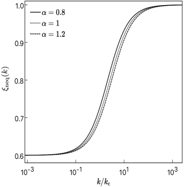
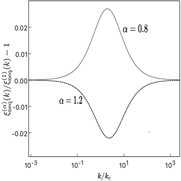
Figure 1: Effect of the parameter $\alpha$ on $\xi_{\mathrm{neq}}(k)$ as defined through Eq. (8) for $\beta=0.6$ and $\lambda=1$. The left panel shows the function $\xi_{\mathrm{neq}}(k)$ for different values of $\alpha$ while the right panel exhibits the fractional difference from the fiducial with $\alpha=1$. For the relevant range (see the fits below), the effect is at best of order a few percent.

The deficit function (8) shares many properties with the Planck-exponential and broken-power laws. To begin with, the long-wavelength limit is

$$\lim_{k\to 0}\xi_{\mathrm{neq}}(k)=\beta,$$ (9)

so that on large scales ($k\ll k_{\mathrm{c}}$) we have

$$\mathcal{P}(k)\underset{k\ll k_{\mathrm{c}}}{\approx}\beta\mathcal{A}_{{}_{\mathrm{S}}}\left(\frac{k}{k_{\star}}\right)^{n_{\mathrm{s}}-1}.$$ (10)

Thus $\xi_{\mathrm{neq}}(k)$ behaves asymptotically like a step function that modifies the spectrum by multiplying it by $\beta$ on large scales and leaving it unchanged on small scales.

The shape of the transition itself depends on both $\alpha$ and $\beta$, which in principle act independently. However, by plotting $\xi_{\mathrm{neq}}(k)$ for different values of $\alpha$ (see Fig. 1) it is easy to see that varying $\alpha$ modifies $\xi_{\mathrm{neq}}(k)$ only during the transition ($k\approx k_{\mathrm{c}}$) and even then only slightly. Figure 1 illustrates this for three values of $\alpha$, specifically 0.8, 1.0 and 1.2 (and with $\beta=0.6$), leading to a difference of at most $\approx 2\%$ in the transition region. We also investigated this effect for other values of $\beta$. For the most extreme cases, namely $\beta\ll 1$ and $\alpha>1.5$ or $\alpha<0.5$, we obtained a maximum difference of order $50\%$ at the transition point.

The additional index $\lambda$ included in (8) permits two different effects (similarly to the expc case). First, in the limit $\beta\to 0$ one finds

$$\xi_{\mathrm{neq}}(k)\big{|}_{\beta\to 0}\underset{k\ll k_{\mathrm{c}}}{\approx}\alpha\sin^{2}\left(\frac{1}{\alpha}\right)\left(\frac{k}{k_{\mathrm{c}}}\right)^{\lambda}.$$ (11)

For this choice of parameters the deficit function $\xi_{\mathrm{neq}}(k)$ changes the spectral index by adding $\lambda$ to the power of $k$. In other words, for large scales $\mathcal{P}(k\to 0)\propto k^{n_{\mathrm{s}}+\lambda-1}$ and we recover the large-scale behavior of the broken power law.

The second effect of $\lambda$ is that it controls the rate of the transition between large and small scales, that is, how many decades it takes for $\xi_{\mathrm{neq}}(k)$ to become approximately constant (numerically saturated to machine precision) for $k>k_{\mathrm{c}}$ and $k<k_{\mathrm{c}}$. For example, the left panel of Fig. 1 shows that $\xi_{\mathrm{neq}}(k)$ is essentially constant as soon as $k/k_{c}\lesssim 10^{-2}$ or $k/k_{c}>10^{2}$. The greater the value of $\lambda$, the faster the transition takes place (this transition is discussed in detail in Appendix B.1). In fact$-$and this will play an important role in our analysis$-$in the limit $\lambda\gg 1$ and with $\beta\not=0$ the deficit function becomes a step function and thus induces a sharp jump in the primordial power spectrum.

In short, using the final parametrization we have the following parameter space

$$(k_{\mathrm{c}},\;\lambda,\;\alpha,\;\beta).$$

The first parameter $k_{\mathrm{c}}$ sets the physical scale at which the transition occurs, $\lambda$ controls the transition rate (and if $\beta=0$ the broken power-law behavior), $\beta$ represents the amplitude of the drop of the power-law spectrum, and $\alpha$ parametrize the shape of the transition (although very weakly).

Given the precision with which the current data (see Refs.Planck Collaboration et al. (2014a); Ade et al. (2016)) can constrain the PPS, we consider three different regions of the parameter space. First we consider the entire space, which we call atan4, and fit all four parameters to the data (following the same nomenclature as for the cases above). In the second parametrization atan3 we restrict attention to the subset $\lambda=1$, so we measure only the position, the rescaling and the shape of the power-law modification. Next we additionally fix $\alpha=1$, yielding the atan2 parametrization with the shape parameter removed. Finally, in the fourth parametrization atan1, we keep $\lambda=1$ and $\alpha=1$ and we additionally impose $\beta=0$, thus measuring only the transition point $k_{\mathrm{c}}$. This last case, as discussed above, shares many characteristics with the broken power law.

When we consider models with some parameters fixed, this is akin to setting a very strong prior (essentially a delta function). Strictly speaking this should be done only in the context of a well-defined theoretical framework. In a purely phenomenological description, it is important to note that results for such restricted models are only illustrative and their statistical significance should not be taken too literally. As we shall see, some of the restricted models perform comparatively well, but their significance might not necessarily be physically meaningful. In general, such restricted fits merely serve to test if a given dataset is able to constrain a given parameter. From the results presented in Tables 1 to 12, we see that for some data combinations all of the parameters are relevant in the sense that leaving them unconstrained improves the fit (showing that the data are sensitive to these parameters), while for other data combinations the extra parameters are irrelevant in the sense that leaving them unconstrained does not improve the fit (showing that the data are not sensitive to these parameters, or equivalently that these parameters are not constrained by the data). In an overall evaluation of the fits, we should avoid the risk of underestimating the $p-$values by considering $p-$values only for models with parameters that the data are actually able to constrain (as studied in detail below).

To complete this overview of the phenomenological models considered in the following analysis, we mention the final one appearing in Tables 1 to 12, which we have dubbed jump. This is a limiting case of the atan function with the rate of transition so large ($\lambda>40,\;\beta\neq 0$) that numerically, at double precision, the transition appears almost discontinuous. This model was not originally included in our list of models. It was added because fitting the quantum relaxation deficit function (8) with a freely-varying sharpness parameter $\lambda$ (as originally suggested in the Planck papers Planck Collaboration et al. (2014a); Ade et al. (2016) for the exponential cutoff and for the broken power-law) led to a value of $\lambda$ much larger than one ($\lambda\gg 1$). Furthermore, starting from a large value $\lambda\approx 50$ the fit was found to be stable for larger values of $\lambda$. This led us to consider a deficit function with a sharp transition, since the function $\xi_{\mathrm{neq}}(k)$ with $\lambda\geq 50$ acts numerically like a discontinuous jump at $k_{c}$. The resulting jump model is then described by the following two-parameter deficit function:

$$\xi_{\mathrm{jump}}(k)=\begin{cases}\beta&\hbox{for}\ \ \ \ k\leq k_{\mathrm{c}},\\ 1&\hbox{for}\ \ \ \ k\geq k_{\mathrm{c}}.\end{cases}$$ (12)

This is the deficit function employed in the tables under the label jump. It has some interesting properties which we discuss in Sec. V.3 below. It is worth emphasising that this new parametrization was found as an extreme case of the atan and expc parametrizations, where the latter as originally introduced in Ref. Contaldi et al. (2003) did not have our extra parameter $\beta$ (where $\beta$ is necessary to obtain the jump model).

II.2 $\Lambda$CDM parameters

Apart from modifying the primordial power spectrum, our adopted cosmology is just the standard six-parameter $\Lambda$CDM model.

In the Planck analyses using CosmoMC Lewis et al. (2000); Lewis (2013), the sampler employs a parametrization with $100\theta_{\mathrm{MC}}$ and $\tau$ instead of $H_{0}$ and $z_{\mathrm{re}}$, since the former are less correlated with the other cosmological parameters. However, this is only an intermediate step. These parameters are then converted to the ones actually used in the numerical computation (this is explained in the CosmoMC documentation and can also be read directly in the code). In our analysis, both the best-fit finder and the Markov Chain Monte Carlo (MCMC) sampler are insensitive to strong correlations between parameters and for this reason we make direct use of the fundamental parametrization with $H_{0}$ and $z_{\mathrm{re}}$, avoiding unnecessary conversions between parametrizations. Note, however, that different parametrizations can have a real influence on the results of an MCMC analysis if flat priors are used. For this reason, when performing the MCMC analysis we used two priors on the parametric space that reduce to simple flat priors for $100\theta_{\mathrm{MC}}$ and $\tau$ when this parametrization is employed.

Apart from the irrelevant difference in parametrization, our cosmological model has the same ingredients as that of Ref. Ade et al. (2016), specifically:

• Hubble constant $H_{0}=100\,h\,\hbox{km}\cdot\hbox{s}^{-1}\cdot\hbox{Mpc}^{-1}$ (thereby defining $h$).

• Electromagnetic background radiation with a fixed temperature today $T_{\gamma 0}=2.7255\,\hbox{K}$.

• One massive neutrino with $m_{\nu}=0.06\,\mathrm{eV}$, vanishing chemical potential, $T_{\nu 0}=0.71611\,T_{\gamma 0}$, and the effective massless neutrino number $N_{\mathrm{eff}}=2.0328$. This configuration is such that when the massive neutrino turns ultra-relativistic, the effective number of massless species is the standard $3.046$.

• Cold dark matter density parametrized by $\Omega_{\mathrm{cdm}}h^{2}$.

• Baryon matter density parametrized by $\Omega_{\mathrm{b}}h^{2}$.

• Spatially flat model $\Omega_{\mathcal{K}}=0$.

• Instantaneous reionization with

  $$\Delta_{\mathrm{HeIII}}=\Delta_{\mathrm{HII}}=0.5,\quad\lambda_{\mathrm{H}}=3/2,$$

  where $\lambda_{\mathrm{H}}$ is the reionization exponent and $\Delta_{\mathrm{HII}}$ is the reionization width (for both HI$\to$HII and HeI$\to$HeII) and $\Delta_{\mathrm{HeIII}}$ is the width for HeII$\to$HeIII. The second reionization HeII$\to$HeIII redshift is kept fixed at $z_{\mathrm{HeIII}}=3.5$. The first reionization redshift is employed as a free parameter $z_{\mathrm{re}}$.

• The fiducial PPS of Eq. (1) with the two free parameters $\mathcal{A}_{{}_{\mathrm{S}}}$ and $n_{\mathrm{s}}$.

• We assume negligible contributions from tensor modes. In practice we set the tensor-to-scalar ratio $r$ to zero (on this point see, however, Sec. V.4).

To summarize, our $\Lambda$CDM model depends on the free parameters

$$\theta_{\Lambda\mathrm{CDM}}=\{H_{0},\;\Omega_{\mathrm{cdm}}h^{2},\;\Omega_{\mathrm{b}}h^{2},\;z_{\mathrm{re}},\;\mathcal{A}_{{}_{\mathrm{S}}},\;n_{\mathrm{s}}\},$$ (13)

in addition to which one must include the PPS modification (2) with the choices (3), (5), (8) or (12) for $\xi(k)$, thus extending the $\Lambda$CDM parameter space $\theta_{\Lambda\mathrm{CDM}}$ by the additional $\theta_{\xi}=\{k_{\mathrm{c}},\;\lambda,\;\alpha,\;\beta\}$ (depending on the case at hand).

As our last ingredient we need the Planck Foreground and Instruments (PFI) parameters (available in Refs. Planck Collaboration et al. (2014b, 2015)), yielding a final extended parameter space

$$\theta=\theta_{\Lambda\mathrm{CDM}}\cup\theta_{\xi}\cup\theta_{\mathrm{PFI}}.$$ (14)

III Methodology

The practical implementation of our methodology is based on specific datasets as detailed in Sec. III.1 together with a statistical analysis as detailed in Sec. III.2.

III.1 Datasets

In our analysis we employ three different CMB datasets (with the same nomenclature as in Ref. Planck Collaboration et al. (2015)). The likelihoods are split into low-$\ell$ [for $\ell\in(2,29)$] and high-$\ell$ (for $\ell\geq 30$). The software adopted is the Planck likelihood code Plik-2.0 (as in Ref. Planck Collaboration et al. (2015)), which implements the Planck likelihood as described in Ref. Planck Collaboration et al. (2016). Our three datasets are as follows:

• Planck $TT$: This refers to the low-$\ell$ and high-$\ell$ likelihoods for CMB temperature anisotropies only (that is, for $C_{\ell}^{TT}$ only). These two likelihoods are labeled by $L_{\mathrm{low}}$ and $L_{\mathrm{high}}$ respectively. The corresponding files for the likelihood code are:

  • low-$\ell$: commander_rc2_v1.1_l2_29_B.clik;

  • high-$\ell$: plik_dx11dr2_HM_v18_TT.clik;

• Planck $TT+$lowP: This includes the polarization data in addition to that of Planck $TT$ for the low-$\ell$ section, specifically $C_{\ell}^{TE}$, $C_{\ell}^{EE}$ and $C_{\ell}^{BB}$ for $\ell\in(2,29)$. Note that we use the symbol $L_{\mathrm{lowP}}$ to refer to the combination of temperature and polarization for low multipoles. The corresponding files for the likelihood code are:

  • low-$\ell$:
    lowl_SMW_70_dx11d_2014_10_03_v5c_Ap.clik;

  • high-$\ell$: plik_dx11dr2_HM_v18_TT.clik;

• Planck $TT$, $TE$, $EE$ + lowP: This includes, in addition to Planck $TT+$lowP, the polarization data $C_{\ell}^{TE}$ and $C_{\ell}^{EE}$ for the high-$\ell$ likelihood. We use the symbol $L_{\mathrm{highP}}$ to refer to this combination of temperature and polarization for high multipoles. The corresponding files for the likelihood code are:

  • low-$\ell$:
    lowl_SMW_70_dx11d_2014_10_03_v5c_Ap.clik;

  • high-$\ell$: plik_dx11dr2_HM_v18_TTTEEE.clik;

Besides the above data likelihoods, the PFI prior is labeled by $L_{\mathrm{PFI}}$ (for simplicity we also use the symbol $L$ here even though this is not a likelihood).

In addition to CMB data we also consider the 2.4% determination of the local value of the Hubble constant Riess et al. (2016). Here we use only their best estimate $H_{0}=73.24\pm 1.74\;\mathrm{km\,sec^{-1}\,Mpc^{-1}}$, labeling it as H0 and its likelihood as $L_{\mathrm{H0}}$. It is worth pointing out that, as discussed in Riess et al. (2016), their likelihood $L(D;H_{0})$ (where $D$ represent the actual data used in Riess et al. (2016)) is well-approximated by a Gaussian, thus in this sense, using a Gaussian prior on $H_{0}$, with the mean and variance as above, is equivalent to using their full dataset. In our analysis we also include BAO derived distances. Here we should stress that, differently from $H_{0}$, a Gaussian likelihood on the BAO derived distances is not equivalent to the full BAO analysis. We employ the Gaussian likelihoods on the distances obtained from the detected BAO signals on the large-scale correlation function as discussed in the papers below:

• galaxies from the 6dF Galaxy Survey (6dFGS) Beutler et al. (2011);

• galaxies with $z<0.2$ from the Sloan Digital Sky Survey (SDSS) Data Release 7 (DR7) Ross et al. (2015);

• galaxies from SDSS DR12 in the redshift interval $0.2<z<0.75$ Alam et al. (2017);

• $147,000$ quasars from the extended Baryon Oscillation Spectroscopic Survey (eBOSS) within $0.8<z<2.2$ Ata et al. (2018);

• $137,562$ quasars with redshifts $2.1\leq z\leq 3.5$ from the DR11 of the BOSS/SDSS-III Delubac et al. (2015);

• cross-correlation of quasars with the Lyman alpha forest absorption, using over 164,000 quasars from DR11 of the BOSS/SDSS-III Font-Ribera et al. (2014);

The combination of all BAO derived data is included in the likelihood $L_{\mathrm{BAO}}$.

III.2 Statistical analysis

In this paper we are interested in answering the following question: assuming that the true PPS is given by $\mathcal{P}_{\mathrm{F}}(k)$, what is the probability that an alternative PPS provides a better fit by pure chance? Our strategy is to calculate this probability considering the whole fit, even though the alternative PPS differs from the (assumed) true PPS mainly on large scales. We use the results of the full fit to study the model quality, including small scales and the other datasets. This avoids any kind of look-elsewhere effect and tackles the problem in a different way. There are many works in the recent literature modeling the large-scale behavior of the CMB anisotropies and trying to obtain a localized signature of a physical process (see for example Ref. Muir et al. (2018) and references therein), whereas in our analysis we also study the compatibility of the modifications with other datasets (as well as their significance).

To discriminate quickly between our models, we first address the problem in a frequentist framework adopting the Likelihood-Ratio Test (LRT) Craig (1984); Hoel (2003). We apply this test by first identifying the full parameter space $\theta$ (see Eq. (14)), where each parametrization of $\xi(k)$ introduced in Sec. II satisfies

$$\lim_{k_{\mathrm{c}}\to 0}\xi(k)=1\quad\Rightarrow\quad\lim_{k_{\mathrm{c}}\to 0}\mathcal{P}(k)=\mathcal{P}_{\mathrm{F}}(k).$$

(For the atan and expc models this also occurs for $\beta=1$). In other words, the fiducial model is nested in the parameter space $\theta$. In the fitting process we use the parameter $q_{\mathrm{c}}=\ln(k_{\mathrm{c}}\times 1\,\mathrm{Mpc})$ (that is numerically, in units of inverse Mpc) instead of $k_{\mathrm{c}}$. This speeds up the numerical fitting process since the parameter $k_{\mathrm{c}}$ can vary by orders of magnitude in a fit. Furthermore, for any value $q_{\mathrm{c}}\ll\ln(H_{0}/c\times 1\,\mathrm{Mpc})$ the deficit function $\xi(k)$ is close to one in the whole physical range of $k$ that influences the CMB anisotropies and is therefore numerically indistinguishable from being taken as exactly one. Thus the fiducial model corresponds to any value of $q_{\mathrm{c}}\ll\ln(H_{0}/c\times 1\,\mathrm{Mpc})$. The maximum likelihood estimator (MLE) for $\theta$ is given by

$$\hat{\theta}=\min_{\theta}\left\{-2\ln\left[L(D|\theta)\right]\right\},$$

where $D$ represents the dataset to be used (in our case Planck $TT$, Planck $TT+$lowP or Planck $TT$, $TE$, $EE$+lowP and their combinations with H0, BAO and H0+BAO), so that $L(D|\theta)$ is given by the appropriate product of

$$L_{\mathrm{low}},\;L_{\mathrm{high}},\;L_{\mathrm{lowP}},\;L_{\mathrm{highP}},\;L_{\mathrm{PFI}},\;L_{\mathrm{H0}},\;L_{\mathrm{BAO}}.$$

On the other hand the MLE for the fiducial subspace is given by

$$\hat{\theta}_{\mathrm{F}}=\min_{\theta_{\mathrm{F}}}\left\{-2\ln\left[L(D|\theta_{\mathrm{F}})\right]\right\},\quad\theta_{\mathrm{F}}\equiv\theta_{\Lambda\mathrm{CDM}}\cup\theta_{\mathrm{PFI}}.$$ (15)

We then introduce the LRT statistic

$$\Gamma\equiv-2\ln\left[\frac{L(D|\hat{\theta}_{\mathrm{F}})}{L(D|\hat{\theta})}\right].$$ (16)

It is easy to convince oneself that $\Gamma\geq 0$ since $L(D|\hat{\theta})\geq L(D|\hat{\theta}_{\mathrm{F}})$. To better understand the effects of $\xi$ in each likelihood we also define the individual ratios

$$\Gamma_{i}\equiv-2\ln\left[\frac{L_{i}(\hat{\theta}_{\mathrm{F}})}{L_{i}(\hat{\theta})}\right],$$ (17)

where $i$ denotes any of (low, lowP, high, highP, BAO, H0, PFI).

In principle if we know $P(\Gamma)$ – the probability distribution of $\Gamma$ – then all we need is to find $\hat{\theta}_{\mathrm{F}}$ and $\hat{\theta}$ in order to compute the probability of obtaining a better fit of $D$ in $\theta$ by chance. This probability is simply given by

$$\gamma=\int_{\Gamma}^{\infty}\mathrm{d}\Gamma^{\prime}P(\Gamma^{\prime}).$$ (18)

Note that we choose the right-hand tail since this corresponds to a $\hat{\theta}$ where the data is more probable than for $\hat{\theta}_{\mathrm{F}}$. In practice, unfortunately, $P(\Gamma)$ is not known and is hardly calculable as it would be impractical to obtain it from first principles given the complexity of the data likelihood. For this reason we must rely on Wilks’ theorem, which asserts that in the large-sample limit $\Gamma$ asymptotically follows a $\chi^{2}_{r}$ distribution (for a proof see Ref. van der Vaart (2000)), where $r$ is the difference in dimensionality between $\theta$ and $\theta_{\mathrm{F}}$. Wilks’ theorem requires the fiducial model to be contained within the parameter space. This is satisfied by the parameter $q_{\mathrm{c}}$ discussed above since the fiducial model requires only that $q_{\mathrm{c}}\ll\ln(H_{0}/c\times 1\,\mathrm{Mpc})$ and/or $\beta=1$. In our parametrizations, the number of free parameters of $\xi(k)$ is 4. We list the critical value of $\Gamma$ corresponding to a $2\sigma$ probability (that is, $95.45\%$) for the relevant cases:

$$\chi^{2}_{1}=4,\quad\chi^{2}_{2}=6.18,\quad\chi^{2}_{3}=8.02,\quad\chi^{2}_{4}=9.72.$$ (19)

In other words, with one extra parameter ($r=1$) a fit giving $\Gamma>4$ means that the fiducial model could only have generated a dataset giving this value of $\Gamma$ (or worse) with a probability below $4.55\%$, and so on for more parameters.

It is worth noting that the LRT has some specific features which are of interest in our case. First, it does not depend on the choice of variables to describe the parameter space $\theta$. Second, it naturally takes into account the difference in the number of parameters when comparing two nested models (see van der Vaart (2000)). An important caveat when using the $\chi^{2}_{r}$ distribution is that it relies on the asymptotic properties of the LRT.

Another aspect of the LRT worth mentioning is that it controls the type-I error, that is, cases where the fiducial model is true but is found to be false. For our choice of $2\sigma$ we would make a type-I error $4.55\%$ of the time. However there is also the type-II error, that is, cases where the alternative model is true but is found to be false. Unlike for the type-I error, the LRT does not provide a simple way to calculate the probability of a type-II error. We could derive this probability analytically if the likelihood was sufficiently simple. But in practice the likelihood is too complicated and one must resort to simulations. A set of simulations of the alternative model must then be produced and, for each simulation, a value of $\{\Gamma_{n}\}$ must be calculated. Using this empirical distribution of $\Gamma$, one can then calculate the probability of a type-II error. In this work we do not address this point. But it is important to bear in mind the possibility that, if a very small critical region is required, one may be significantly increasing the type-II error. This would be the case, for example, if one were requiring $5\sigma$ instead of $2\sigma$.

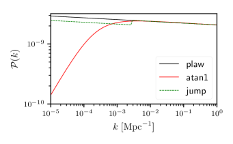
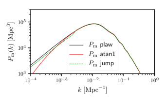
Figure 2: Upper panel: best-fit power spectra with the most successful deficit functions (see text). It is clear that for a smooth transition the relevant scale at which the deficit becomes significant is of order the Hubble radius, whereas in the almost discontinuous case (with a large value of $\lambda$) the transition scale is an order of magnitude smaller. Lower panel: the corresponding matter power spectra. Only the case of a sharp transition remains close to the case of a fiducial spectrum. It is an open question to understand if and how such a slight difference could be observable in future data. These fits are for the full Planck dataset.

As is clear from the above discussion, the difference in the number of parameters between the fiducial and alternative models is crucial in determining the significance of the result [see Eq. (19)]. Moreover, the use of a $\chi^{2}_{r}$ distribution is based on the large-sample asymptotic limit. For this reason we note that, if a parameter controls a region of the model where there are almost no data, then we do not expect the asymptotic regime to be attained. For example, consider the parameter $\alpha$ discussed in Sec. II. It modifies the PPS only in a rather narrow band of $k$ around $k_{\mathrm{c}}$, and it also modifies the PPS only slightly at this point. Consequently, we expect this parameter to be very degenerate and not to contribute much to the fit. In an extreme case where the alternative model has a parameter that does not modify the PPS fit at all, it is reasonable to assume that the current data are not able to shed any light on that aspect of the model. In such a case we also perform the statistical tests with the degenerate parameter removed from the analysis (keeping it fixed at some fiducial value), and we do not take that parameter into account when comparing the alternative and fiducial models. This ambiguity in the number of parameters is a natural feature of our phenomenological approach. Thus the two relevant questions are: what kind of modification of the fiducial model is the data able to fit, and what is the significance of this fit?

$\xi(k)$	$k_{\mathrm{c}}^{-1}[\mathrm{Gpc}]$	$\lambda$	$\beta$	$\alpha$	$h$	$n_{\mathrm{s}}$	$\ln(10^{10}\mathcal{A}_{{}_{\mathrm{S}}})$	$\tau$	$\Gamma$	$\Gamma_{\mathrm{low}}$	$\Gamma_{\mathrm{high}}$	$\gamma$
plaw	–	–	–	–	$0.69$	$0.98$	$3.2$	$0.15$	$0$	$0$	$0$	–
bpl	$2.9$	$7.9$	–	–	$0.69$	$0.98$	$3.2$	$0.14$	$2.7$	$2.9$	$-0.04$	$26$% ($1.1\sigma$) $[2]$
atan1	$3.6$	$1$	$0$	$1$	$0.7$	$0.97$	$3.3$	$0.18$	$5.5$	$4.4$	$1$	$1.9$% ($2.4\sigma$) $[1]$
atan2	$1.4$	$1$	$0.49$	$1$	$0.7$	$0.97$	$3.4$	$0.22$	$5.8$	$5.2$	$0.44$	$5.5$% ($1.9\sigma$) $[2]$
atan3	$1.7$	$1$	$0.47$	$0.94$	$0.7$	$0.97$	$3.3$	$0.2$	$5.9$	$5$	$0.7$	$12$% ($1.6\sigma$) $[3]$
atan4	$0.36$	$41$	$0.79$	$0.58$	$0.69$	$0.98$	$3.3$	$0.16$	$6.9$	$6.3$	$0.57$	$14$% ($1.5\sigma$) $[4]$
expc1	$2.1$	$0.5$	$0$	–	$0.69$	$0.98$	$3.3$	$0.18$	$5.6$	$4.7$	$0.8$	$1.8$% ($2.4\sigma$) $[1]$
expc2	$2.7$	$0.44$	$0$	–	$0.69$	$0.98$	$3.3$	$0.17$	$5.8$	$4.9$	$0.83$	$5.4$% ($1.9\sigma$) $[2]$
expc3	$0.33$	$14$	$0.78$	–	$0.69$	$0.98$	$3.3$	$0.17$	$6.7$	$6.2$	$0.43$	$8.1$% ($1.7\sigma$) $[3]$
jump	$0.36$	–	$0.78$	–	$0.69$	$0.98$	$3.3$	$0.17$	$6.8$	$6.3$	$0.34$	$3.4$% ($2.1\sigma$) $[2]$

Table 1: Best-fits and their significance obtained with the Planck $TT$ dataset. For each model we present the best-fit values of the cutoff scale $k_{\mathrm{c}}^{-1}$ in Gpc and the values of the dimensionless parameters $\lambda$, $\beta$ and $\alpha$. We also include the best-fit values of some of the $\Lambda$CDM parameters, namely, the dimensionless rescaled Hubble scale $h$, the spectral index $n_{\mathrm{s}}$ and amplitude $A_{\mathrm{s}}$ of the fiducial PPS (1), and finally the reionization optical depth $\tau$ derived from the best-fit. We present the significance in two ways: the LRT statistics $\Gamma$ defined by (16) (including the individual $\Gamma_{i}$ defined for each likelihood included in the final one) and (in the last column) the $p-$value $\gamma$ defined by (18) (where we also include the probability $\gamma$ translated into the corresponding number of one-dimensional Gaussian standard deviations).

$\xi(k)$	$k_{\mathrm{c}}^{-1}[\mathrm{Gpc}]$	$\lambda$	$\beta$	$\alpha$	$h$	$n_{\mathrm{s}}$	$\ln(10^{10}\mathcal{A}_{{}_{\mathrm{S}}})$	$\tau$	$\Gamma$	$\Gamma_{\mathrm{low}}$	$\Gamma_{\mathrm{high}}$	$\Gamma_{H0}$	$\gamma$
plaw	–	–	–	–	$0.7$	$0.98$	$3.2$	$0.16$	$0$	$0$	$0$	$0$	–
bpl	$2.8$	$7.6$	–	–	$0.7$	$0.99$	$3.2$	$0.16$	$2.6$	$2.3$	$0.03$	$0.3$	$27$% ($1.1\sigma$) $[2]$
atan1	$3$	$1$	$0$	$1$	$0.71$	$0.98$	$3.4$	$0.21$	$7.1$	$3.8$	$1.8$	$1.4$	$0.79$% ($2.7\sigma$) $[1]$
atan2	$1.3$	$1$	$0.5$	$1$	$0.71$	$0.97$	$3.4$	$0.23$	$8.3$	$4.8$	$1.6$	$1.8$	$1.6$% ($2.4\sigma$) $[2]$
atan3	$1.3$	$1$	$0.51$	$1$	$0.71$	$0.97$	$3.4$	$0.23$	$8.2$	$4.8$	$1.6$	$1.8$	$4.1$% ($2\sigma$) $[3]$
atan4	$1.3$	$1$	$0.51$	$0.99$	$0.71$	$0.97$	$3.4$	$0.23$	$8.3$	$4.8$	$1.6$	$1.8$	$8.1$% ($1.8\sigma$) $[4]$
expc1	$1.5$	$0.5$	$0$	–	$0.71$	$0.99$	$3.4$	$0.22$	$6.9$	$4.3$	$1$	$1.5$	$0.85$% ($2.6\sigma$) $[1]$
expc2	$1.6$	$0.36$	$0$	–	$0.72$	$0.98$	$3.4$	$0.24$	$8.6$	$4.8$	$1.4$	$2.2$	$1.4$% ($2.5\sigma$) $[2]$
expc3	$1.6$	$0.36$	$0.007$	–	$0.72$	$0.98$	$3.4$	$0.24$	$8.6$	$4.8$	$1.4$	$2.2$	$3.6$% ($2.1\sigma$) $[3]$
jump	$0.35$	–	$0.76$	–	$0.7$	$0.99$	$3.3$	$0.2$	$7.2$	$5.9$	$0.76$	$0.57$	$2.8$% ($2.2\sigma$) $[2]$

Table 2: The same as Table 1 but with Planck $TT$ + H0.

$\xi(k)$	$k_{\mathrm{c}}^{-1}[\mathrm{Gpc}]$	$\lambda$	$\beta$	$\alpha$	$h$	$n_{\mathrm{s}}$	$\ln(10^{10}\mathcal{A}_{{}_{\mathrm{S}}})$	$\tau$	$\Gamma$	$\Gamma_{\mathrm{low}}$	$\Gamma_{\mathrm{high}}$	$\Gamma_{\mathrm{BAO}}$	$\gamma$
plaw	–	–	–	–	$0.68$	$0.97$	$3.2$	$0.14$	$0$	$0$	$0$	$0$	–
bpl	$2.8$	$8$	–	–	$0.68$	$0.97$	$3.2$	$0.13$	$2.6$	$2.8$	$-0.13$	$-0.01$	$27$% ($1.1\sigma$) $[2]$
atan1	$3.5$	$1$	$0$	$1$	$0.69$	$0.97$	$3.3$	$0.18$	$4.6$	$4.1$	$0.41$	$-0.18$	$3.2$% ($2.1\sigma$) $[1]$
atan2	$2$	$1$	$0.48$	$1$	$0.69$	$0.96$	$3.3$	$0.18$	$5$	$5$	$0.09$	$-0.18$	$8.1$% ($1.7\sigma$) $[2]$
atan3	$2$	$1$	$0.48$	$1$	$0.69$	$0.96$	$3.3$	$0.18$	$5$	$5$	$0.09$	$-0.18$	$17$% ($1.4\sigma$) $[3]$
atan4	$0.35$	$48$	$0.77$	$0.51$	$0.69$	$0.98$	$3.3$	$0.18$	$5.5$	$6.5$	$-0.16$	$-1.1$	$24$% ($1.2\sigma$) $[4]$
expc1	$2.2$	$0.5$	$0$	–	$0.69$	$0.97$	$3.3$	$0.16$	$5.3$	$4.7$	$0.52$	$-0.02$	$2.1$% ($2.3\sigma$) $[1]$
expc2	$2.5$	$0.45$	$0$	–	$0.69$	$0.97$	$3.3$	$0.17$	$5.5$	$4.9$	$0.46$	$0.02$	$6.4$% ($1.9\sigma$) $[2]$
expc3	$0.33$	$20$	$0.79$	–	$0.69$	$0.97$	$3.3$	$0.16$	$6.7$	$6.4$	$0.14$	$-0.02$	$8.3$% ($1.7\sigma$) $[3]$
jump	$0.36$	–	$0.79$	–	$0.68$	$0.97$	$3.3$	$0.16$	$6.8$	$6.4$	$0.22$	$0.03$	$3.4$% ($2.1\sigma$) $[2]$

Table 3: The same as Table 1 but with Planck $TT$ + BAO.

$\xi(k)$	$k_{\mathrm{c}}^{-1}[\mathrm{Gpc}]$	$\lambda$	$\beta$	$\alpha$	$h$	$n_{\mathrm{s}}$	$\ln(10^{10}\mathcal{A}_{{}_{\mathrm{S}}})$	$\tau$	$\Gamma$	$\Gamma_{\mathrm{low}}$	$\Gamma_{\mathrm{high}}$	$\Gamma_{H0}$	$\Gamma_{\mathrm{BAO}}$	$\gamma$
plaw	–	–	–	–	$0.69$	$0.98$	$3.2$	$0.13$	$0$	$0$	$0$	$0$	$0$	–
bpl	$3$	$7.9$	–	–	$0.69$	$0.98$	$3.2$	$0.14$	$2.6$	$2.2$	$0.34$	$0.08$	$-0.05$	$27$% ($1.1\sigma$) $[2]$
atan1	$3.9$	$1$	$0$	$1$	$0.69$	$0.97$	$3.3$	$0.17$	$5.6$	$3.5$	$1.6$	$0.8$	$-0.53$	$1.8$% ($2.4\sigma$) $[1]$
atan2	$2.6$	$1$	$0.49$	$1$	$0.69$	$0.97$	$3.3$	$0.17$	$5.8$	$4$	$1.3$	$0.94$	$-0.62$	$5.6$% ($1.9\sigma$) $[2]$
atan3	$1.4$	$1$	$0.5$	$0.54$	$0.69$	$0.97$	$3.3$	$0.17$	$5.8$	$4$	$1.4$	$0.79$	$-0.5$	$12$% ($1.5\sigma$) $[3]$
atan4	$0.35$	$46$	$0.77$	$0.52$	$0.69$	$0.98$	$3.3$	$0.18$	$6.5$	$5.6$	$0.58$	$0.63$	$-0.46$	$16$% ($1.4\sigma$) $[4]$
expc1	$2.1$	$0.5$	$0$	–	$0.69$	$0.98$	$3.3$	$0.18$	$5.8$	$3.8$	$1.4$	$0.63$	$-0.37$	$1.6$% ($2.4\sigma$) $[1]$
expc2	$2.5$	$0.44$	$0$	–	$0.69$	$0.98$	$3.3$	$0.18$	$6$	$4.1$	$1.4$	$0.48$	$-0.2$	$4.9$% ($2\sigma$) $[2]$
expc3	$0.33$	$17$	$0.77$	–	$0.69$	$0.98$	$3.3$	$0.18$	$6.5$	$5.5$	$0.7$	$0.55$	$-0.38$	$8.8$% ($1.7\sigma$) $[3]$
jump	$0.35$	–	$0.77$	–	$0.69$	$0.98$	$3.3$	$0.18$	$6.7$	$5.6$	$0.76$	$0.31$	$-0.14$	$3.5$% ($2.1\sigma$) $[2]$

Table 4: The same as Table 1 but with Planck $TT$ + H0 + BAO.

$\xi(k)$	$k_{\mathrm{c}}^{-1}[\mathrm{Gpc}]$	$\lambda$	$\beta$	$\alpha$	$h$	$n_{\mathrm{s}}$	$\ln(10^{10}\mathcal{A}_{{}_{\mathrm{S}}})$	$\tau$	$\Gamma$	$\Gamma_{\mathrm{low}}$	$\Gamma_{\mathrm{high}}$	$\gamma$
plaw	–	–	–	–	$0.68$	$0.97$	$3.1$	$0.085$	$0$	$0$	$0$	–
bpl	$1.2$	$0.68$	–	–	$0.68$	$0.97$	$3.1$	$0.1$	$2.1$	$0.9$	$1.1$	$34$% ($0.95\sigma$) $[2]$
atan1	$5.3$	$1$	$0$	$1$	$0.68$	$0.96$	$3.2$	$0.11$	$3.5$	$2.3$	$1.1$	$6.2$% ($1.9\sigma$) $[1]$
atan2	$5.2$	$1$	$0.01$	$1$	$0.68$	$0.96$	$3.1$	$0.1$	$3.5$	$2.4$	$1.1$	$17$% ($1.4\sigma$) $[2]$
atan3	$3.7$	$1$	$0.009$	$0.52$	$0.68$	$0.96$	$3.1$	$0.1$	$3.6$	$2.1$	$1.4$	$30$% ($1\sigma$) $[3]$
atan4	$0.38$	$37$	$0.81$	$0.51$	$0.68$	$0.97$	$3.1$	$0.11$	$5$	$3$	$1.9$	$29$% ($1.1\sigma$) $[4]$
expc1	$2.9$	$0.5$	$0$	–	$0.68$	$0.97$	$3.2$	$0.11$	$3.9$	$1.8$	$1.9$	$5$% ($2\sigma$) $[1]$
expc2	$2.7$	$0.52$	$0$	–	$0.68$	$0.97$	$3.2$	$0.11$	$3.9$	$1.8$	$1.8$	$14$% ($1.5\sigma$) $[2]$
expc3	$0.35$	$14$	$0.8$	–	$0.68$	$0.97$	$3.2$	$0.11$	$4.7$	$2.5$	$1.9$	$19$% ($1.3\sigma$) $[3]$
jump	$0.37$	–	$0.81$	–	$0.68$	$0.97$	$3.1$	$0.1$	$5.1$	$3.1$	$1.7$	$8$% ($1.8\sigma$) $[2]$

Table 5: The same as Table 1 but with Planck $TT$ + lowP.

$\xi(k)$	$k_{\mathrm{c}}^{-1}[\mathrm{Gpc}]$	$\lambda$	$\beta$	$\alpha$	$h$	$n_{\mathrm{s}}$	$\ln(10^{10}\mathcal{A}_{{}_{\mathrm{S}}})$	$\tau$	$\Gamma$	$\Gamma_{\mathrm{lowP}}$	$\Gamma_{\mathrm{high}}$	$\Gamma_{H0}$	$\gamma$
plaw	–	–	–	–	$0.69$	$0.97$	$3.1$	$0.093$	$0$	$0$	$0$	$0$	–
bpl	$1.2$	$0.71$	–	–	$0.69$	$0.98$	$3.1$	$0.11$	$2.9$	$1$	$0.85$	$0.89$	$23$% ($1.2\sigma$) $[2]$
atan1	$5.6$	$1$	$0$	$1$	$0.69$	$0.97$	$3.2$	$0.11$	$3.8$	$1.6$	$1.6$	$0.49$	$5.1$% ($1.9\sigma$) $[1]$
atan2	$5.4$	$1$	$0.007$	$1$	$0.69$	$0.97$	$3.2$	$0.11$	$3.9$	$1.6$	$1.8$	$0.38$	$15$% ($1.5\sigma$) $[2]$
atan3	$3.6$	$1$	$0.003$	$0.5$	$0.69$	$0.97$	$3.2$	$0.12$	$4.1$	$1$	$2.4$	$0.5$	$25$% ($1.2\sigma$) $[3]$
atan4	$0.38$	$41$	$0.81$	$0.56$	$0.69$	$0.97$	$3.2$	$0.11$	$4.7$	$2$	$3.2$	$-0.68$	$32$% ($0.99\sigma$) $[4]$
expc1	$3.2$	$0.5$	$0$	–	$0.69$	$0.97$	$3.2$	$0.12$	$4$	$1.1$	$2.3$	$0.3$	$4.6$% ($2\sigma$) $[1]$
expc2	$2.7$	$0.57$	$0$	–	$0.69$	$0.97$	$3.2$	$0.12$	$4.1$	$1.1$	$2.3$	$0.41$	$13$% ($1.5\sigma$) $[2]$
expc3	$0.36$	$14$	$0.81$	–	$0.69$	$0.97$	$3.2$	$0.12$	$4.5$	$1$	$3.6$	$-0.44$	$21$% ($1.2\sigma$) $[3]$
jump	$0.37$	–	$0.81$	–	$0.69$	$0.97$	$3.2$	$0.12$	$4.6$	$1$	$2.9$	$0.3$	$10$% ($1.6\sigma$) $[2]$

Table 6: The same as Table 1 but with Planck $TT$ + lowP + H0.

$\xi(k)$	$k_{\mathrm{c}}^{-1}[\mathrm{Gpc}]$	$\lambda$	$\beta$	$\alpha$	$h$	$n_{\mathrm{s}}$	$\ln(10^{10}\mathcal{A}_{{}_{\mathrm{S}}})$	$\tau$	$\Gamma$	$\Gamma_{\mathrm{lowP}}$	$\Gamma_{\mathrm{high}}$	$\Gamma_{\mathrm{BAO}}$	$\gamma$
plaw	–	–	–	–	$0.68$	$0.97$	$3.1$	$0.088$	$0$	$0$	$0$	$0$	–
bpl	$1.2$	$0.63$	–	–	$0.68$	$0.97$	$3.1$	$0.096$	$2.3$	$1.2$	$1.1$	$0.06$	$31$% ($1\sigma$) $[2]$
atan1	$5.3$	$1$	$0$	$1$	$0.68$	$0.96$	$3.2$	$0.11$	$3.5$	$1.8$	$1.7$	$0.08$	$6$% ($1.9\sigma$) $[1]$
atan2	$5.3$	$1$	$0$	$1$	$0.68$	$0.96$	$3.2$	$0.11$	$3.5$	$1.8$	$1.7$	$0.08$	$17$% ($1.4\sigma$) $[2]$
atan3	$5.3$	$1$	$0$	$1$	$0.68$	$0.96$	$3.2$	$0.11$	$3.5$	$1.8$	$1.7$	$0.08$	$32$% ($1\sigma$) $[3]$
atan4	$0.37$	$46$	$0.82$	$0.52$	$0.68$	$0.97$	$3.2$	$0.11$	$4.6$	$2.4$	$1.9$	$0.14$	$33$% ($0.97\sigma$) $[4]$
expc1	$3$	$0.5$	$0$	–	$0.68$	$0.97$	$3.2$	$0.11$	$3.8$	$1.6$	$2$	$0.05$	$5$% ($2\sigma$) $[1]$
expc2	$3$	$0.53$	$0$	–	$0.68$	$0.97$	$3.1$	$0.11$	$3.9$	$2.1$	$1.6$	$0.08$	$14$% ($1.5\sigma$) $[2]$
expc3	$0.35$	$17$	$0.8$	–	$0.68$	$0.97$	$3.2$	$0.12$	$4.4$	$1.6$	$2.4$	$0.1$	$22$% ($1.2\sigma$) $[3]$
jump	$0.37$	–	$0.8$	–	$0.68$	$0.97$	$3.2$	$0.12$	$4.3$	$1.4$	$2.6$	$0.11$	$11$% ($1.6\sigma$) $[2]$

Table 7: The same as Table 1 but with Planck $TT$ + lowP + BAO.

$\xi(k)$	$k_{\mathrm{c}}^{-1}[\mathrm{Gpc}]$	$\lambda$	$\beta$	$\alpha$	$h$	$n_{\mathrm{s}}$	$\ln(10^{10}\mathcal{A}_{{}_{\mathrm{S}}})$	$\tau$	$\Gamma$	$\Gamma_{\mathrm{lowP}}$	$\Gamma_{\mathrm{high}}$	$\Gamma_{H0}$	$\Gamma_{\mathrm{BAO}}$	$\gamma$
plaw	–	–	–	–	$0.69$	$0.97$	$3.1$	$0.098$	$0$	$0$	$0$	$0$	$0$	–
bpl	$1.2$	$0.69$	–	–	$0.69$	$0.97$	$3.1$	$0.1$	$2.9$	$2.5$	$0.14$	$0.34$	$-0.12$	$24$% ($1.2\sigma$) $[2]$
atan1	$5.7$	$1$	$0$	$1$	$0.69$	$0.97$	$3.1$	$0.1$	$3.9$	$3.8$	$0.02$	$0.17$	$0.01$	$4.9$% ($2\sigma$) $[1]$
atan2	$5.7$	$1$	$0$	$1$	$0.69$	$0.97$	$3.1$	$0.1$	$3.9$	$3.8$	$0.02$	$0.17$	$0.01$	$14$% ($1.5\sigma$) $[2]$
atan3	$5.7$	$1$	$0$	$1$	$0.69$	$0.97$	$3.1$	$0.1$	$3.9$	$3.8$	$0.03$	$0.17$	$0.01$	$27$% ($1.1\sigma$) $[3]$
atan4	$0.38$	$42$	$0.82$	$0.52$	$0.69$	$0.97$	$3.2$	$0.11$	$5$	$3.5$	$1.1$	$0.43$	$-0.15$	$29$% ($1.1\sigma$) $[4]$
expc1	$3.1$	$0.5$	$0$	–	$0.69$	$0.97$	$3.2$	$0.11$	$4.2$	$2.9$	$1.1$	$0.17$	$0$	$4$% ($2\sigma$) $[1]$
expc2	$3.1$	$0.5$	$0$	–	$0.69$	$0.97$	$3.2$	$0.11$	$4.2$	$2.9$	$1.1$	$0.17$	$0$	$12$% ($1.6\sigma$) $[2]$
expc3	$0.36$	$16$	$0.81$	–	$0.69$	$0.97$	$3.2$	$0.12$	$4.7$	$2.6$	$1.7$	$0.3$	$-0.05$	$19$% ($1.3\sigma$) $[3]$
jump	$0.37$	–	$0.81$	–	$0.69$	$0.97$	$3.2$	$0.12$	$4.8$	$2.5$	$1.8$	$0.3$	$-0.04$	$9.2$% ($1.7\sigma$) $[2]$

Table 8: The same as Table 1 but with Planck $TT$ + lowP + H0 + BAO.

The standard Bayesian approach in this case uses the Bayes factor

$$B_{\textsc{fa}}=\frac{\displaystyle\int\mathrm{d}\theta\;L(D|\hat{\theta})P(\theta)}{\displaystyle\int\mathrm{d}\theta_{\mathrm{F}}\;L(D|\hat{\theta}_{\mathrm{F}})P_{\mathrm{F}}(\theta_{\mathrm{F}})},$$ (20)

where $P_{\mathrm{F}}$ and $P$ are the respective priors in the fiducial and alternative models. As in Ref. Ade et al. (2016), if we consider the same flat prior for both models ($P_{\mathrm{F}}(\theta_{\mathrm{F}})=1$ and $P(\theta)=1$, besides the PFI priors cited above), the LRT gives us a point estimate of the Bayes factor:

$$B_{\textsc{fa}}\approx\exp\left(\frac{\Gamma}{2}\right).$$

In this work we do not initially follow the Bayesian approach for all the models for two reasons. First, as we stated above, in this phenomenological study we want to understand the ability of the current data to inform us about different aspects of the model, whereas a Bayesian approach would simply tend to penalize any irrelevant extra parameters in the alternative model. Our initial interest is in determining if those extra parameters should be included in the analysis. The second reason why we initially perform a frequentist analysis stems, again, from the phenomenological nature of our approach: we may not have any theoretical reason to assume a specific prior for the extra parameters, and in fact even a flat prior would not be unambiguous since it depends on the choice of parameters. Note that the frequentist approach does not depend on the introduction of a measure in the model space (usually done through simple priors in the model parameters).

A frequentist approach does not answer the same questions as a Bayesian methodology. All we can know in a frequentist study is the ability of the current data to falsify the fiducial model (the null hypothesis). In other words, if an alternative model provides a better fit to the data$-$one that goes beyond the improvement expected from statistical fluctuations and from the addition of extra parameters$-$then we may say that the fiducial model is falsified. Since we will be evaluating a large number of cases, we chose to first follow the frequentist approach, thereby answering the simplest questions while avoiding the introduction of a measure in the model space. We then apply a follow-up Bayesian analysis to what appears to be the best competing model.

In our Bayesian approach we run a complete MCMC analysis of the posteriors of the fiducial and competing models using an ensemble sampler algorithm that was introduced in Ref. Goodman and Weare (2010) and which is here implemented in NumCosmo as described in Appendix A. From the results we produce a corner plot containing the marginal distributions and two-dimensional confidence regions for all relevant parameters. We then apply the modified harmonic mean, also described in Appendix A, to estimate the Bayes factor resulting from the comparison of the fiducial and competing models.

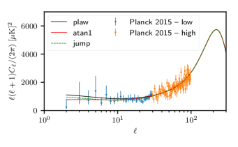
Figure 3: Examples of best-fit CMB anisotropies with the different deficit functions (see text), together with the Planck 2015 $TT$ data up to $\ell=100$ (this limit is chosen for aesthetic reasons). The smooth transition represented by atan1 results in a larger deficit at the lower multipoles ($\ell=$2–10), whereas jump results in a deficit which is smaller at these lower multipoles and larger at the higher multipoles $\ell=$20–30. This reveals the difference between the sharp and the smooth deficit. The latter improves the fit at the lowest multipoles only, while the former also affects the spectrum around $\ell=$20–30 where the cosmic variance is less important. These fits are for the full Planck dataset.

We emphasize that the main objective of this paper is to compute the value of $\Gamma$ for each alternative model (and $\Gamma_{i}$ for each component of the final likelihood). The value of $B_{\textsc{fa}}$ is computed only for the jump model. Naturally, we also obtain the best-fit parameters and (from the MCMC analysis) the full posterior. While a parameter-space analysis can be useful to understand the behavior of a model, this is not our main objective.

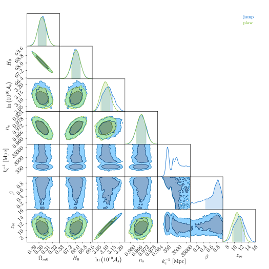
Figure 4: Corner plot for the MCMC results with plaw and jump using the full Planck dataset, H0 and BAO. The marginal distribution for $k_{\mathrm{c}}^{-1}$ has three modes: the first at $\sim 380$ Mpc, the second at $\sim 1450$ Mpc and the third at $\sim 3200$ Mpc. As expected the distribution for $k_{\mathrm{c}}^{-1}$ becomes flat for $k_{\mathrm{c}}^{-1}\gtrsim 3200\mathrm{Mpc}$, since at these values the jump mode is numerically equivalent to plaw. Furthermore, in this interval, the distribution for $\beta$ becomes completely degenerate as can be seen in the $k_{\mathrm{c}}^{-1}\times\beta$ confidence region. This is the reason why the short-distance mode appears to provide a definite set of values and may therefore be considered physically relevant, while the second and third (long-distance) modes are too degenerate in the actual value of the amplitude of the jump (not to mention that the scale induced is very close to the Hubble scale). Thus we do not consider these modes any further.

IV Numerical approach

The theoretical CMB anisotropies $C^{XY}_{\ell}$ do not depend on the Planck foreground and instrument parameters in $\theta_{\mathrm{PFI}}$. For this reason we divide the problem of finding the best fit into two steps. In the first step, we define the full Planck likelihood $L(D|\theta)$ as a function on the whole parameter space. Fixing the values of $\{\theta_{\Lambda\mathrm{CDM}},\theta_{\xi}\}$, we can cheaply calculate the likelihood for different points of $\theta_{\mathrm{PFI}}$ since we can re-use the same $C^{XY}_{\ell}$. We then define the PFI-Likelihood as

$$L_{\mathrm{PFI}}\left(D|\theta_{\Lambda\mathrm{CDM}},\theta_{\xi}\right)=\max_{\theta_{\mathrm{PFI}}}L(D|\theta).$$ (21)

In the second step, we find the maximum of $L_{\mathrm{PFI}}\left(D|\theta_{\Lambda\mathrm{CDM}},\theta_{\xi}\right)$. Since these two steps are mathematically equivalent (when the likelihood is $C^{\infty}$ in the parameters), we can use them to speed up significantly the finding of the best fit. Furthermore, in a multimodal likelihood (which is frequently the case for high-dimensional likelihoods) the fitting process can always stop prematurely for two reasons. First, if it finds a local maximum. Second, if it is moving in a plateau where the likelihood varies slowly (that is, where it has a very small gradient). There is no known algorithm that could guarantee that the true maximum has been found. Thus we have applied the usual checking method of starting the fitting process from different initial points in the parametric space in order to minimize this risk. The specific objects and methods used at this stage are described in Appendix A.

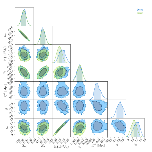
Figure 5: Corner plot for the MCMC results from plaw and jump using the full Planck dataset, H0 and BAO and removing the second and third modes (see Fig. 4). In this plot we use a linear scale for $k_{\mathrm{c}}^{-1}$. Note that once the second mode is removed, there is a shift in $\mathcal{A}_{\mathrm{s}}$ and $z_{\mathrm{re}}$. This was already present in Fig 4, in the $k_{\mathrm{c}}^{-1}\times\log(10^{10}\mathcal{A}_{\mathrm{s}})$ and $k_{\mathrm{c}}^{-1}\times z_{\mathrm{re}}$ confidence regions, where the one-sigma contour related to the second mode of $k_{\mathrm{c}}^{-1}$ is slightly shifted when compared to the first mode. In addition, we have a negative correlation for $k_{\mathrm{c}}^{-1}\times\beta$: a smaller jump scale $k_{\mathrm{c}}^{-1}$ implies a smaller jump amplitude ($\beta$ closer to unity).

For the computation of $C^{XY}_{\ell}$ we employed the Class back end of NumCosmo (see Refs. Blas et al. (2011); Lesgourgues (2011); Lesgourgues and Tram (2011)). The precision settings were increased compared to the default configuration; further details can be found in Appendix A. It suffices to note here that, in order to measure differences between primordial power spectra, we considered three different precision settings: low precision (LP) (equal to the default setting in CLASS, as in their version 2.5.0), medium precision (MP), and high precision (HP). Increasing the precision from low to medium changes the results in some cases (with $\Delta\Gamma\approx 0.5$), but the results then remain stable when the precision is further increased to the highest level. We therefore report results obtained with medium precision.

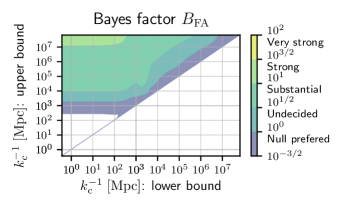
Figure 6: Bayesian evidence comparing jump and plaw models for various combinations of upper and lower bounds on the $k_{\mathrm{c}}^{-1}$ prior. This analysis used the full Planck dataset, H0 and BAO-derived distances. The white areas represent forbidden regions (lower bound greater than upper bound) or regions without enough points in the sample. To the right of the graph we include the evidence scale (Jeffreys’ scale) proposed in Ref. (Jeffreys, 1998, Appendix B).

V Results

We group our results according to which CMB data we are using. For a given CMB sample we discuss its results alone and in combination with the other samples H0, BAO and H0+BAO. We already know from previous studies (see for example Ade et al. (2016) and references therein) that there is a lack of power on large scales for the temperature data. However, studying this effect alone can be misleading as it is difficult to take into account the look-elsewhere effect when we are dealing with a large and heterogeneous body of data. We therefore compare the whole fit when using different datasets, and we also include the differences in the fit for each relevant part of the likelihood. This analysis of the significance of the different deficit models suggests that most of them are not sufficiently competitive to justify a complete MCMC analysis of their parametric space.

V.1 General considerations

We summarize our results in Tables 1 to 12. For each parametrization and dataset used, we show the best-fit values of the cutoff scale $k_{\mathrm{c}}^{-1}$ in Gpc and (when relevant) the values of the dimensionless parameters $\lambda$, $\beta$ and $\alpha$. The first ($\lambda$) measures the sharpness of the deficit function, the second ($\beta$) quantifies the deficit, while the third ($\alpha$) describes the shape of the transition. After these four new parameters we include the best-fit values of the four standard parameters: the dimensionless rescaled Hubble scale $h$, the spectral index $n_{\mathrm{s}}$ and amplitude $A_{\mathrm{s}}$ of the fiducial PPS (1), and finally the reionization optical depth $\tau$ (which is computed as a derived quantity from the best-fit values). To complete the tables we add the LRT statistics $\Gamma$ defined by (16) and (in the last column) the $p-$value $\gamma$ defined by (18). To the last column we add (in round brackets) the probability $\gamma$ translated into the corresponding number of one-dimensional Gaussian standard deviations, and also (in square brackets) the number of extra degrees of freedom. It is often assumed that a $p-$value of 5% indicates statistical significance. We shall here instead take the view that whenever a small value is found, this merely suggests a plausible new effect.

In the first line of Table 9 we reproduce the currently accepted values for the four standard-model parameters $h$, $n_{\mathrm{s}}$, $A_{\mathrm{s}}$ and $\tau$, where our fit matches that provided by the Planck team (see, however, App A).

The first conclusion one can draw from the tables is that the standard-model parameters are hardly affected by the inclusion of the deficit function, regardless of the choice of the latter. This shows that even if the lack of power is a true physical phenomenon, it cannot come from a strong effect as otherwise the analysis would have shown some instability when including this phenomenon in the description of the data. This also immediately shows that there is no chance of resolving the $H_{0}$ tension by taking the deficit function into account. Such a possibility might be considered upon examining Table 2, where we see that a reasonable amount of the significance is produced by a better fitting of the H0 data (see $\Gamma_{H0}$). However, this effect is severely reduced when polarization data are added. In other words, when fitting $TT$ data alone the extra freedom in the PPS seems to allow a better fit of the $TT$ + H0 data combination, but this does not hold when polarization data are added. On the contrary, comparing with the plaw fits including H0, we see that when polarization data (at both low-$\ell$ and high-$\ell$) are added we get $-2\ln(L_{H0})\approx 9$, which corresponds roughly to the well-known $3\sigma$ tension with the H0 data. For this reason, our results including H0 should be interpreted with caution.

V.2 The smooth deficit functions

Throughout the data, if we set the interval for the parameter $\lambda$ to be around unity (that is, if we impose a smooth transition), it is found that the best-fit value of the transition scale remains very close to the Hubble radius (in terms of $k^{-1}$, corresponding to a length scale one order of magnitude larger than the Hubble radius) – where the data are dominated by cosmic variance. As a result, these fits are only marginally significant (like those originally discussed by the Planck team). Adding data for polarization, H0 and the BAO’s does not change this trend, and in fact adding polarization actually reduces the significance.

Our weakly-significant fits neither support nor rule out the smooth deficit functions we have studied. Statistically speaking, according to our frequentist analysis, these functions are more or less as successful as the standard power-law model (taking into account the larger number of parameters). This result might be viewed as a modest success, in the sense that a smooth deficit could have been disfavored compared to no deficit but instead performs comparably well. On the other hand, the data we have studied are consistent with the apparent low power being a mere statistical fluctuation. In the absence of a significantly better fit for the models with a smooth deficit, it is also natural to invoke Ockham’s razor to favor the simpler model with no extra parameters (even if, strictly speaking, no such conclusion can be drawn on the basis of the significance of the fits).

Furthermore, the data we have studied certainly cannot constrain the shape of the smooth-deficit spectrum even if it exists. This seems to be so regardless of the functional form of the deficit function (expc, bpl or atan), and independently of the number of extra parameters and priors assumed. This conclusion is compatible with our result that the shape parameter $\alpha$ is essentially irrelevant. Roughly speaking, we found $\alpha$ ranging between $\frac{1}{2}$ and 1. As shown in Fig. 1, this amounts to hardly any variation at all in the actual spectrum. Thus it appears that the data cannot favor any particular shape.

$\xi(k)$	$k_{\mathrm{c}}^{-1}[\mathrm{Gpc}]$	$\lambda$	$\beta$	$\alpha$	$h$	$n_{\mathrm{s}}$	$\ln(10^{10}\mathcal{A}_{{}_{\mathrm{S}}})$	$\tau$	$\Gamma$	$\Gamma_{\mathrm{lowP}}$	$\Gamma_{\mathrm{highP}}$	$\gamma$
plaw	–	–	–	–	$0.67$	$0.97$	$3.1$	$0.082$	$0$	$0$	$0$	–
bpl	$0.21$	$0.14$	–	–	$0.67$	$0.96$	$3.1$	$0.1$	$4.7$	$2.6$	$1.9$	$9.6$% ($1.7\sigma$) $[2]$
atan1	$6.5$	$1$	$0$	$1$	$0.67$	$0.96$	$3.1$	$0.094$	$3.4$	$2.8$	$0.65$	$6.7$% ($1.8\sigma$) $[1]$
atan2	$6.5$	$1$	$0$	$1$	$0.67$	$0.96$	$3.1$	$0.094$	$3.4$	$2.8$	$0.82$	$19$% ($1.3\sigma$) $[2]$
atan3	$6.5$	$1$	$0.003$	$0.98$	$0.67$	$0.96$	$3.1$	$0.094$	$3.4$	$2.8$	$0.76$	$34$% ($0.96\sigma$) $[3]$
atan4	$0.38$	$31$	$0.82$	$0.7$	$0.67$	$0.96$	$3.1$	$0.091$	$5.7$	$4.3$	$1.3$	$22$% ($1.2\sigma$) $[4]$
expc1	$3.4$	$0.5$	$0$	–	$0.67$	$0.96$	$3.1$	$0.1$	$4$	$2.4$	$1.6$	$4.5$% ($2\sigma$) $[1]$
expc2	$2.7$	$0.57$	$0$	–	$0.67$	$0.96$	$3.1$	$0.099$	$4.2$	$2.3$	$1.8$	$13$% ($1.5\sigma$) $[2]$
expc3	$0.35$	$13$	$0.82$	–	$0.67$	$0.96$	$3.1$	$0.096$	$5.7$	$3.8$	$1.7$	$13$% ($1.5\sigma$) $[3]$
jump	$0.38$	–	$0.82$	–	$0.67$	$0.96$	$3.1$	$0.093$	$5.8$	$4.2$	$1.5$	$5.5$% ($1.9\sigma$) $[2]$

Table 9: The same as Table 1 but with Planck $TT$, $TE$, $EE$ + lowP.

$\xi(k)$	$k_{\mathrm{c}}^{-1}[\mathrm{Gpc}]$	$\lambda$	$\beta$	$\alpha$	$h$	$n_{\mathrm{s}}$	$\ln(10^{10}\mathcal{A}_{{}_{\mathrm{S}}})$	$\tau$	$\Gamma$	$\Gamma_{\mathrm{lowP}}$	$\Gamma_{\mathrm{highP}}$	$\Gamma_{H0}$	$\gamma$
plaw	–	–	–	–	$0.68$	$0.97$	$3.1$	$0.089$	$0$	$0$	$0$	$0$	–
bpl	$0.22$	$0.14$	–	–	$0.68$	$0.97$	$3.1$	$0.1$	$4.8$	$2.5$	$2.1$	$-0.01$	$9.2$% ($1.7\sigma$) $[2]$
atan1	$7.3$	$1$	$0$	$1$	$0.68$	$0.96$	$3.1$	$0.096$	$3.2$	$3$	$0.33$	$0.01$	$7.4$% ($1.8\sigma$) $[1]$
atan2	$6.8$	$1$	$0.022$	$1$	$0.68$	$0.96$	$3.1$	$0.098$	$3.2$	$2.9$	$0.66$	$-0.11$	$20$% ($1.3\sigma$) $[2]$
atan3	$4.8$	$1$	$0.005$	$0.51$	$0.68$	$0.96$	$3.1$	$0.094$	$3.3$	$3.2$	$0.23$	$0.02$	$35$% ($0.93\sigma$) $[3]$
atan4	$0.39$	$31$	$0.82$	$0.77$	$0.68$	$0.97$	$3.1$	$0.099$	$5.5$	$3.7$	$1.6$	$-0.06$	$24$% ($1.2\sigma$) $[4]$
expc1	$3.7$	$0.5$	$0$	–	$0.68$	$0.97$	$3.1$	$0.1$	$4.1$	$2.4$	$1.6$	$0.08$	$4.2$% ($2\sigma$) $[1]$
expc2	$2.8$	$0.58$	$0$	–	$0.68$	$0.97$	$3.1$	$0.1$	$4.2$	$2.3$	$1.6$	$0.2$	$12$% ($1.5\sigma$) $[2]$
expc3	$0.36$	$14$	$0.82$	–	$0.68$	$0.97$	$3.1$	$0.1$	$5.5$	$3.3$	$2.2$	$-0.32$	$14$% ($1.5\sigma$) $[3]$
jump	$0.39$	–	$0.82$	–	$0.68$	$0.97$	$3.1$	$0.095$	$5.3$	$4.1$	$0.99$	$0.08$	$7.1$% ($1.8\sigma$) $[2]$

Table 10: The same as Table 1 but with Planck $TT$, $TE$, $EE$ + lowP + H0.

$\xi(k)$	$k_{\mathrm{c}}^{-1}[\mathrm{Gpc}]$	$\lambda$	$\beta$	$\alpha$	$h$	$n_{\mathrm{s}}$	$\ln(10^{10}\mathcal{A}_{{}_{\mathrm{S}}})$	$\tau$	$\Gamma$	$\Gamma_{\mathrm{lowP}}$	$\Gamma_{\mathrm{highP}}$	$\Gamma_{\mathrm{BAO}}$	$\gamma$
plaw	–	–	–	–	$0.68$	$0.97$	$3.1$	$0.085$	$0$	$0$	$0$	$0$	–
bpl	$0.23$	$0.14$	–	–	$0.68$	$0.97$	$3.1$	$0.1$	$4.7$	$2.3$	$2.2$	$-0.03$	$9.4$% ($1.7\sigma$) $[2]$
atan1	$7$	$1$	$0$	$1$	$0.68$	$0.96$	$3.1$	$0.095$	$3.2$	$2.9$	$0.59$	$-0.08$	$7.4$% ($1.8\sigma$) $[1]$
atan2	$7$	$1$	$0.013$	$1$	$0.68$	$0.96$	$3.1$	$0.097$	$3.2$	$2.7$	$0.73$	$-0.15$	$20$% ($1.3\sigma$) $[2]$
atan3	$4.4$	$1$	$0.002$	$0.51$	$0.68$	$0.96$	$3.1$	$0.094$	$3.4$	$3$	$0.86$	$-0.25$	$33$% ($0.97\sigma$) $[3]$
atan4	$0.37$	$32$	$0.82$	$0.68$	$0.68$	$0.97$	$3.1$	$0.1$	$5.5$	$3.5$	$1.9$	$-0.06$	$24$% ($1.2\sigma$) $[4]$
expc1	$3.5$	$0.5$	$0$	–	$0.68$	$0.97$	$3.1$	$0.1$	$4.1$	$2.4$	$2$	$-0.28$	$4.3$% ($2\sigma$) $[1]$
expc2	$2.8$	$0.59$	$0$	–	$0.68$	$0.97$	$3.1$	$0.1$	$4.1$	$2.2$	$1.8$	$0.06$	$13$% ($1.5\sigma$) $[2]$
expc3	$0.35$	$14$	$0.81$	–	$0.68$	$0.97$	$3.1$	$0.1$	$5.4$	$3.4$	$1.8$	$0.09$	$15$% ($1.5\sigma$) $[3]$
jump	$0.38$	–	$0.83$	–	$0.68$	$0.97$	$3.1$	$0.093$	$5.3$	$4.2$	$1.1$	$-0.07$	$7.1$% ($1.8\sigma$) $[2]$

Table 11: The same as Table 1 but with Planck $TT$, $TE$, $EE$ + lowP + BAO.

$\xi(k)$	$k_{\mathrm{c}}^{-1}[\mathrm{Gpc}]$	$\lambda$	$\beta$	$\alpha$	$h$	$n_{\mathrm{s}}$	$\ln(10^{10}\mathcal{A}_{{}_{\mathrm{S}}})$	$\tau$	$\Gamma$	$\Gamma_{\mathrm{lowP}}$	$\Gamma_{\mathrm{highP}}$	$\Gamma_{H0}$	$\Gamma_{\mathrm{BAO}}$	$\gamma$
plaw	–	–	–	–	$0.68$	$0.97$	$3.1$	$0.095$	$0$	$0$	$0$	$0$	$0$	–
bpl	$0.23$	$0.15$	–	–	$0.68$	$0.97$	$3.2$	$0.11$	$4.7$	$2.7$	$1.7$	$0.11$	$0.01$	$9.7$% ($1.7\sigma$) $[2]$
atan1	$6.6$	$1$	$0$	$1$	$0.68$	$0.96$	$3.1$	$0.099$	$3.2$	$4$	$-0.28$	$-0.16$	$-0.04$	$7.1$% ($1.8\sigma$) $[1]$
atan2	$6.6$	$1$	$0$	$1$	$0.68$	$0.96$	$3.1$	$0.099$	$3.3$	$4$	$-0.26$	$-0.16$	$-0.04$	$20$% ($1.3\sigma$) $[2]$
atan3	$6.6$	$1$	$0$	$1$	$0.68$	$0.96$	$3.1$	$0.099$	$3.3$	$4$	$-0.24$	$-0.16$	$-0.04$	$35$% ($0.93\sigma$) $[3]$
atan4	$0.39$	$32$	$0.82$	$0.76$	$0.68$	$0.97$	$3.1$	$0.1$	$5.4$	$4.6$	$1.3$	$-0.4$	$-0.09$	$25$% ($1.2\sigma$) $[4]$
expc1	$3.7$	$0.5$	$0$	–	$0.68$	$0.97$	$3.1$	$0.1$	$4$	$3.5$	$0.51$	$0.02$	$0$	$4.6$% ($2\sigma$) $[1]$
expc2	$2.6$	$0.6$	$0$	–	$0.68$	$0.97$	$3.1$	$0.11$	$4.3$	$2.9$	$1.2$	$0.12$	$0.01$	$12$% ($1.6\sigma$) $[2]$
expc3	$0.36$	$14$	$0.81$	–	$0.68$	$0.97$	$3.1$	$0.1$	$5.3$	$4.5$	$1.4$	$-0.5$	$-0.13$	$15$% ($1.4\sigma$) $[3]$
jump	$0.38$	–	$0.83$	–	$0.68$	$0.97$	$3.1$	$0.095$	$5.1$	$5.1$	$0.23$	$-0.17$	$-0.02$	$7.7$% ($1.8\sigma$) $[2]$

Table 12: The same as Table 1 but with Planck $TT$, $TE$, $EE$ + lowP + H0 + BAO.

V.3 The jump function

Having found that a smooth transition to large-scale low power does not improve the fit to a degree that is convincingly significant, we now consider the extreme case of a sharp transition. More precisely, we discuss a transition that is so fast that the data are incapable of discerning its structure. Statistically speaking one could argue, from the results in our Tables, that the jump case is not necessarily preferable to some of our other models such as atan1 or expc1. However, one should bear in mind that the latter cases correspond to imposing strong (delta function) priors on the extra parameters and with no particular physical justification (though see Sec. VI for a possible physical motivation for atan1). Moreover, as a careful investigation of the Tables reveals, the jump model appears to be remarkably stable with respect to the dataset considered, in contrast with the other models. In particular, the values of the jump parameters vary little from one dataset to another (the statistical significance of the fit being also somewhat more stable). Finally it should be emphasized that, starting from a smooth transition, the likelihood minimization procedure itself naturally leads us to a sharp transition. It is in this sense that we view the jump deficit proposal as being suggested in an especially natural way by the data.

In Fig. 2 we show the difference between the sharp jump deficit and the smooth plaw and atan1 deficits, together with the consequences for the matter power spectrum $P_{\mathrm{m}}(k)$. Figure 3 shows that, when translated into CMB anisotropies, the jump deficit decreases the $C_{\ell}$’s at larger multipoles than is the case for the smooth deficits plaw and atan1. Specifically, jump produces a larger angular-power deficit in the region $\ell=$20–30.

As we have noted, the case of a sharp transition exhibits an intriguing stability across our datasets. For $C_{\ell}^{TT}$ only, we obtain a variation of less than 2% for the best-fit characteristic scale $k_{\mathrm{c}}^{-1}$, which is found to range from 353 to 361 Mpc, and we find a best-fit dip in power down to between 76 and 79% (that is, we find $\beta$ between 0.76 and 0.79). The $p-$value is around 3%.

Including the polarization for the low multipoles increases the $p-$value to around 10%, while increasing the scale $k_{\mathrm{c}}^{-1}$ to about 370 Mpc and leaving the dip $\beta$ essentially unchanged at around 0.80 or 80%. With the full polarization data the scale is pushed upward even more, reaching about 380 Mpc, while the dip reaches 83% at most and the $p-$value is lowered to 7%. Thus it would appear from the data that we are unable to unambiguously assert the existence of a new characteristic length scale, although our analysis naturally points to one. Even so, as shown in Figs. 4 and 5, this variation in the value of the scale is well within the error bar for $k_{\mathrm{c}}^{-1}$.

Finally, we have computed the Bayes factor for the comparison of jump and plaw using our full dataset (Planck $TT$, $TE$, $EE$ + lowP, H0 and BAO-derived distances). As stated before, we use flat priors for the cosmological parameters together with the PFI priors. For nested models, the priors of the common parameters do not change the final Bayes factor (see for instance Ref. Trotta (2007)). The only relevant priors are those for the new parameters:

$$-1\leq\ln\left(\frac{k_{\mathrm{c}}^{-1}}{1\;\mathrm{Mpc}}\right)\leq 18,\qquad 0\leq\beta\leq 1.$$

Instead of reporting a single value for $B_{\textsc{fa}}$ for the above priors, we adopt the framework of a robust Bayesian analysis. The prior of $\beta$ is chosen so that all possible deficits are allowed and are equally probable. However, there is no clear way to choose a meaningful interval for the prior of $\ln(k_{\mathrm{c}})$. We circumvent this problem by calculating the Bayes factor for all subintervals of $-1\leq\ln\left(\displaystyle\frac{k_{\mathrm{c}}^{-1}}{1\;\mathrm{Mpc}}\right)\leq 18$ and plotting the results in Fig. 6, thereby showing the sensitivity to the prior. The Bayes factor for the full interval is found to be

$$B_{\textsc{fa}}=10^{1.06}=11.5.$$

This is considered “strong” on the Jeffreys’ scale given in Ref. (Jeffreys, 1998, Appendix B).

In Fig. 6 there is no interval where the evidence is “decisive” or “very strong”, although in a large portion of the graph the Bayes factor is classified as “strong”. On the other hand, the figure shows that to achieve “strong” evidence it is necessary to include all peaks or the last two peaks and part of the plateau in the distribution of $k_{\mathrm{c}}^{-1}$ be allowed by the prior (see Fig. 4). For priors including only one peak, the evidence drops to “substantial”. Thus a conservative conclusion is that we have only “substantial” evidence for a particular scale (at $k_{\mathrm{c}}^{-1}\simeq 380\;\mathrm{Mpc}$).

V.4 Tensor modes and scalar-tensor consistency

In our data analysis we have ignored tensor modes (effectively assuming a negligible tensor-to-scalar ratio $r\simeq 0$). It is however noteworthy that, for both atan and expc as well as for jump, we have found a general degradation of the frequentist significance when polarization data are added (though noting that the parameters remain remarkably stable for jump). The pattern of degradation depends on the datasets considered. For example, comparing $TT$ only (Table 1) with the full Planck data (Table 9) the degradation of $p-$values for atan is worse than for jump, while comparing $TT$ + BAO (Table 3) with $TT$ + BAO + lowP (Table 7) the degradation is worse for jump. For $TT$ + BAO and full Planck + BAO (Table 11) the degradations are comparable. On the other hand it should be noted that the $\Gamma$ values are persistently higher for jump, indicating that the degradation is less severe. To explain these observations, we may consider three possible scenarios.

First, we may imagine that we are in fact simply modeling a statistical fluke. This would imply that the more data we add, the smaller the resulting significance. However, this does not generally appear to be the case. Although there seems to be a systematic decrease in significance of the fits when we add polarization data, adding other datasets does not result in any particular systematic (positive or negative) trend for the fits.

A second possibility is that our models are indeed fitting a real feature but also partially overfitting statistical fluctuations (a combination of cosmic variance, sample variance and data noise). In this case, adding more data may be expected to wash out the overfit simply by reducing the variance, and this in turn would reduce the significance to its genuine value. For each of our deficit functions it can then happen that, because of an overfitting of the datasets without polarization, significance is lost when polarization data are added. If this turns out to be the true explanation for the observed degradation, then jump will arguably be the preferred deficit function because of its persistently high values of $\Gamma$ (though in terms of $p-$values it is not clear which function would be preferred).

The third scenario, which we focus on in this section, is related to the assumption of negligible tensor contributions. This is arguably something of a theoretical prejudice, stemming from the $\Lambda$CDM + inflation paradigm with a small value of $r$ (specifically $r_{0.002}<0.099$, with 95% CL from temperature and polarization data), the relevant constraint being calculated within that framework. In contrast with this paradigmatic case, Ref Ade et al. (2016) fitted several variants. For instance, allowing the possibility of a running spectral index for the scalar PPS, the upper bound on $r$ becomes $r_{0.002}<0.15$ (95% CL, with temperature and polarization data). Thus changing the framework (for example allowing for a running spectral index) permits us to relax the constraint on $r$. Including a deficit function in the PPS can be even more drastic as it can break the inflationary scalar-tensor consistency. In the context of our analysis it is therefore natural to expect that a larger tensor contribution is allowed. We are then led to consider that the addition of a tensor contribution, with a breaking of scalar-tensor consistency, might enable us to avoid the degradation noted above. If this turns out to be the true explanation for the observed degradation, then atan will arguably be the preferred deficit function because (as discussed below) quantum relaxation models naturally allow for a breaking of scalar-tensor consistency.

The $TT$ angular power spectra are functionals of the scalar ($\mathcal{P}_{\textsc{s}}$) and tensor ($\mathcal{P}_{\textsc{t}}$) power spectra:

$$C_{\ell}^{TT}=C_{\textsc{s},\ell}^{TT}[\mathcal{P}_{\textsc{s}}]+C_{\textsc{t},\ell}^{TT}[\mathcal{P}_{\textsc{t}}]\ .$$ (22)

We may parametrize $\mathcal{P}_{\textsc{t}}$ with an amplitude $\mathcal{A}_{\textsc{t}}=r\mathcal{A}_{\textsc{s}}$ and write $\mathcal{P}_{\textsc{s}}=\mathcal{A}_{\textsc{s}}f(k)$ and $\mathcal{P}_{\textsc{t}}=r\mathcal{A}_{\textsc{s}}g(k)$. Since the functionals are linear we have

$$C_{\ell}^{TT}=A_{\textsc{s}}C_{\textsc{s},\ell}^{TT}[f]+rA_{\textsc{s}}C_{\textsc{t},\ell}^{TT}[g].$$ (23)

Our polarization angular power spectra are also linear functionals of $\mathcal{P}_{\textsc{s}}$ and $\mathcal{P}_{\textsc{t}}$ and so similarly we have

$$C_{\ell}^{XY}=A_{\textsc{s}}C_{\textsc{s},\ell}^{XY}[f]+rA_{\textsc{s}}C_{\textsc{t},\ell}^{XY}[g],$$ (24)

where $X$ and $Y$ can denote the possible polarizations $E$ and $B$ (as well as the temperature $T$). If $r$ is very small, the total values of $C_{\ell}^{XY}$ (including $C_{\ell}^{TT}$) will be determined essentially by $\mathcal{P}_{\textsc{s}}$ only.

Now the data seem to show anomalously low values of $C_{\ell}^{TT}$ for $\ell$ roughly in the interval $[2,50]$. If we modify the function $f(k)$ appropriately we can improve our fit to the $TT$ data in this region. However, it is not so straightforward if we consider a dataset that includes polarization. For example, if we take the datasets $TT$ and $TE+EE$, the component $TE+EE$ does not have the same anomalously low power at low $\ell$. Thus if we try modifying $f(k)$ so as to improve the fit to the $TT$ data, at some point we will worsen the fit to the $TE+EE$ data. In other words, with a total likelihood

$$\ln L_{\mathrm{total}}=\ln L_{TT}[A_{\textsc{s}},f]+\ln L_{TE+EE}[A_{\textsc{s}},f],$$ (25)

lowering the power in $f$ will increase the first term but decrease the second, so that the best fit will be somewhere in the middle ground.

If instead the tensor contribution is not negligible on all scales of interest, it may be possible to increase $\ln L_{TT}[A_{\textsc{s}},r,f,g]$ without decreasing $\ln L_{TE+EE}[A_{\textsc{s}},r,f,g]$ – provided we are allowed to vary the functions $f$ and $g$ independently. For then we might be able to choose $f$ such that we have lower power in $C_{\ell}^{TT}$ on large scales while at the same time choosing $g$ such that it compensates for the lower power in $C_{\ell}^{TE}$ and $C_{\ell}^{EE}$ at large scales (resulting from lower values of $C_{\textsc{s},\ell}^{TE}[f]$ and $C_{\textsc{s},\ell}^{EE}[f]$) and without spoiling the rest of the fit. This would require the relative tensor contributions to $TE$ and $EE$ to be larger than the relative tensor contribution to $TT$, which can occur in appropriate conditions.

However, to vary $f$ and $g$ independently amounts to a violation of scalar-tensor consistency. In such conditions the definition

$$r\equiv 4\frac{\mathcal{P}_{\textsc{t}}}{\mathcal{P}_{\textsc{s}}}$$ (26)

of $r$ is no longer a fixed number but will generally depend on $k$. In practice, however, $r$ is taken to be the ratio (26) at the pivot scale $k=k_{\ast}$ (with $\mathcal{A}_{\textsc{s}}$ defined as the value of $\mathcal{P}_{\textsc{s}}$ at $k=k_{\ast}$ so that $f=1$ at that point), in which case the general relations (23) and (24) are still valid. Note that while this scenario requires a large contribution from tensor modes at large scales, $r$ itself could still be small since it is defined at the relatively small pivot scale.

This reasoning suggests that, if the low-power anomaly in $C_{\ell}^{TT}$ is real, then having significant tensor contributions at large scales (with a violation of scalar-tensor consistency) might allow us to avoid a degradation of the fit when polarization data are included.

An intriguing feature of quantum relaxation models is that they naturally imply a large-scale violation of scalar-tensor consistency without spoiling the overall inflationary scenario Valentini (2010). This is because, when the initial conditions are no longer constrained by the Born rule, there is no reason why different degrees of freedom should have the same initial nonequilibrium distribution and hence there is no reason why they should have the same large-scale deficit function $\xi(k)$. In general we will have two distinct functions $\xi_{\textsc{s}}(k)$ and $\xi_{\textsc{t}}(k)$ for scalar and tensor modes respectively, with two different and unequal sets of parameters $\alpha_{\textsc{s}}$, $\beta_{\textsc{s}}$, $(k_{\mathrm{c}})_{\textsc{s}}$ and $\alpha_{\textsc{t}}$, $\beta_{\textsc{t}}$, $(k_{\mathrm{c}})_{\textsc{t}}$ (with $\lambda=1$ throughout). A more complete data analysis would then require a fit to this six-parameter model, where for completeness $r$ itself could also be subject to a fresh fit. Such studies are left for future work.

VI Implications for quantum relaxation models

In this section we consider the implications of our data analysis for quantum relaxation models Colin and Valentini (2015, 2016, 2013); Valentini (2010).

VI.1 Best-fit results for the nonequilibrium deficit

As noted in Sec. II.1, quantum relaxation during a radiation-dominated preinflationary era (combined with a simplifying assumption about the transition to inflation) predicts an approximate deficit function $\xi_{\mathrm{neq}}(k)$ of the form (6) with $\lambda=1$ Colin and Valentini (2015, 2016). That is, the relaxation scenario predicts the deficit function that we have here called atan3, with three undetermined parameters $\alpha$, $\beta$ and $k_{\mathrm{c}}$. In the present analysis we have fitted the data to atan3, and also to the reduced functions atan2 (with $\alpha=1$) and atan1 (with $\alpha=1$ and $\beta=0$). The results show that conclusions about the fits depend on the datasets considered, in particular on whether we consider only datasets with no polarization (Tables 1–4) or whether we instead consider only datasets that include polarization (Tables 5–12).

As a general point of principle, it could happen that a useful pattern emerges only for datasets that include polarization. More complete datasets can be required to observe an effect, where more data generally implies smaller error bars (by diminishing the data variance). In this spirit it may be useful to consider Tables 1–4 and Tables 5–12 as two distinct sets of data.

VI.1.1 Best fit without polarization

If we restrict ourselves to datasets without polarization, for a reliable best fit atan1 does not suffice and we require atan2 or atan3.

To see this, observe that in Tables 1–4 the parameter $k_{\mathrm{c}}$ changes considerably from atan1 to atan2 (where the latter fit yields quite a large $\beta\simeq 0.5$), showing that atan1 is not a reliable fit. Thus, while atan1 shows an apparently impressive significance of up to $2.7\sigma$ (Table 2) for these data sets, the instability of the fit indicates that this result should be discounted. Whereas, again for Tables 1–4, the parameters $k_{\mathrm{c}}$ and $\beta$ are more or less stable from atan2 to atan3 (although less stable for Table 4), suggesting that atan2 is a reliable fit – with a significance of up to $2.4\sigma$ (Table 2). The latter result is suggestive, but as we shall discuss the significance diminishes when polarization data are included.

VI.1.2 Best fit including polarization

If instead we ignore datasets without polarization, we find that the only relevant parameter is the (uncertain) scale $k_{\mathrm{c}}$, so that the best-fit function is in effect just atan1. However, we cannot really conclude that $\beta=0$ because the data cannot provide such a constraint. In other words, the likelihood (for atan2 and atan3) is almost constant around $\beta=0$ (see Tables 5–12). This is a direct consequence of $\beta$ modifying the spectrum only at values of $k^{-1}$ much larger than $k_{\mathrm{c}}^{-1}$ (as discussed in Sec. B.1): since $k_{\mathrm{c}}^{-1}$ is already large, $\beta$ modifies the spectrum at unobservable scales. To obtain an upper bound on $\beta$, we could vary the initial $\beta$ values in the fitting process making them closer and closer to one (or we could perform a full MCMC posterior analysis). For the purpose of model comparison, however, it suffices to obtain the fits with $\beta\approx 0$.

VI.1.3 Significance of atan1

If we consider all the datasets, we find, as a rough general trend, that the more data we add the larger the best-fit lengthscale $k_{\mathrm{c}}^{-1}$ and the smaller the significance of the fit. This suggests that the effect is probably a statistical fluctuation. In principle, however, it could be that the effect only occurs at super-Hubble scales and that the atan1 model is trying to fit a real physical feature there. With this in mind, if we allow ourselves to disregard the datasets without polarization (and if we fix $\lambda=1$ as in the quantum relaxation model), then it is reasonable to consider only atan1 since at these scales neither $\alpha$ nor $\beta$ have a measurable impact on the spectrum. Thus atan1 may be regarded as a smooth alternative to the sharp function jump. For datasets including polarization, atan1 is found to have a significance of up to only $2\sigma$ (Table 8).

VI.1.4 Degradation and stability of fits. Comparison with jump

From the point of view of significance atan1 performs about as well as jump (overall for datasets including polarization both at low- and high-$\ell$), having in some cases a slightly better significance for the same dataset. However, the significance of atan1 is found to diminish systematically as more polarization data are included (see Table XIII), that is, including polarization at low-$\ell$ decreases the significance and when both low- and high-$\ell$ are included the significance decreases even further. By contrast, while the significance of jump decreases when low-$\ell$ polarization is added it increases again for the full polarization data (see Table XIV). Both deficit functions have a significance varying from $\approx 1.5\sigma$ to $\approx 2.5\sigma$.

Regarding the general stability of the fits, as discussed in Ref. Kandhadai and Valentini (in preparation) there are different regions of the atan parameter space that produce approximately the same curve. Such degeneracy can result in a large variation and apparent instability of the best-fit parameters for atan. In contrast, for jump there can be no such degeneracy. As we have seen the parameters for jump are found to be stable, and this of course implies that the function itself is stable. This fact, together with the larger values of $\Gamma$ for jump, motivated our follow-up Bayesian analysis carried out above. The case for running a similar Bayesian analysis for atan is not as strong: the stability of the function remains to be clarified as does the structure of the parameter space, and in any case the values of $\Gamma$ are lower. Thus we leave such further analysis for future work.

VI.2 Quantum relaxation and future work

We now comment on the implications of our results for future work on quantum relaxation models.

VI.2.1 Mechanism for negligible super-Hubble power

As far as $p-$values are concerned, atan1 performs more or less as well as jump (for datasets including polarization). This motivates us to ask if there might be a theoretical model that predicts atan1 and in particular a near-vanishing $\beta$. Because $\beta=\lim_{k\rightarrow 0}\xi_{\mathrm{neq}}(k)$, this means that we require a model in which the primordial power spectrum itself becomes negligible in the far super-Hubble limit.

In a quantum relaxation scenario with a radiation-dominated preinflationary phase, the limit $k\rightarrow 0$ yields the maximum suppression or “freezing” of quantum relaxation. As shown in Sec. V of Ref. Colin and Valentini (2013), in the far super-Hubble regime the de Broglie-Bohm time evolution of a field mode on an interval $(t_{\mathrm{i}},t_{\mathrm{f}})$ with $t_{\mathrm{f}}\gg t_{\mathrm{i}}$ is equivalent to the time evolution of a standard harmonic oscillator on a time interval $(t_{\mathrm{i}},3t_{\mathrm{i}})$. Thus for $k\rightarrow 0$ all modes effectively evolve over the same small time $2t_{\mathrm{i}}$ and we expect very limited relaxation. At small $k$ the resulting deficit function $\xi_{\mathrm{neq}}(k)$ will then be essentially equal to the deficit function $\xi_{\mathrm{ic}}(k)$ associated with the initial conditions. This means that, for long-wavelength modes, the freezing of relaxation preserves the initial conditions almost intact. A negligible value of $\beta$ then implies a negligible statistical variance (or power) in the initial conditions themselves (for modes in the far super-Hubble regime).

This motivates us to consider a quantum relaxation scenario in which there is negligible super-Hubble noise in the initial state (corresponding to very small $\beta$). It is a matter for future theoretical work to develop the details of such a scenario. A simple suggestion is to assume that there is negligible power in the initial conditions for all modes. This is an attractive hypothesis, as physically it means that essentially all of the quantum noise we observe at later times was generated dynamically.

While the hypothesis of negligible initial power provides a good physical reason to prefer atan1, so far the significance remains small. A full MCMC analysis might help to evaluate whether or not it is worth pursuing such models. This would depend on the resulting upper bound on $\beta$.

If this hypothesis is considered further, it would be natural to apply the same reasoning to tensor modes as well, in which case we would expect the distinct functions $\xi_{\textsc{s}}(k)$ and $\xi_{\textsc{t}}(k)$ (discussed in Sec. V.4) to each take the form of atan1 but with different scales $(k_{\mathrm{c}})_{\textsc{s}}$ and $(k_{\mathrm{c}})_{\textsc{t}}$ (again generally breaking scalar-tensor consistency).

VI.2.2 Other signatures of quantum relaxation

The data seem to show that if there is a low-power anomaly it must exist at large scales that we cannot accurately measure. Because cosmic variance is so large in the relevant region, we are unable to meaningfully test the predictions of quantum relaxation for the power deficit alone. To improve the chances of constraining such models we need to include more detailed predictions$-$such as primordial oscillations and statistical anisotropy, which are additional generic features of quantum relaxation. Extensive numerical simulations show significant oscillations around the atan function Colin and Valentini (2015, 2016), which have however so far eluded a simple and general parametrization. Statistical anisotropy arises from initial nonequilibrium distributions that depend on the direction $\bm{\hat{k}}$ of the wave vector, resulting in parameters $\alpha$, $\beta$, $k_{\mathrm{c}}$ that depend on $\bm{\hat{k}}$, where the effect of $\alpha(\bm{\hat{k}})$ could arguably persist at large $\ell$ and hence have a more visible impact on the data Valentini (2015).

VI.2.3 Quantum relaxation across the transition

Finally, it should be emphasised that the atan prediction was obtained on the simplifying assumption that the transition does not affect the nonequilibrium distribution left at the end of a radiation-dominated preinflationary era Colin and Valentini (2015). Modeling the transition and simulating the time evolution of nonequilibrium across it remains to be done. How this might change the overall result is currently unknown. The evidence discussed above in favor of a sudden jump deficit raises the question of whether or not a realistic quantum relaxation model could yield such a result (or, indeed, if such a result could arise from other kinds of models not involving quantum relaxation).

VII Conclusions

A smooth deficit function can be superimposed on the primordial power spectrum to mimic the large-scale deficit which has apparently been observed in some cosmological data. We have analyzed a broad range of data using different parametrized versions of the deficit function, in such a way as to be able to compare with a previous analysis by the Planck team. We confirm that, for the deficit functions we consider, the fit is only marginally better than for the standard power law, where the improvement occurs at wavelengths comparable to the Hubble scale. It would appear that, taken by itself, the power deficit is not very statistically significant and therefore not necessarily physical. This result is consistent with previous investigations. We do, however, find some suggestive hints for future work.

We have consistently found hints of statistically-significant fits, only to find that the significance degrades when polarization data are added. We have argued that such degradation might be avoided in models that break scalar-tensor consistency and which have non-negligible tensor contributions at large scales. Quantum relaxation models in fact naturally break scalar-tensor consistency, yielding independent deficit functions for scalar and tensor degrees of freedom. Fitting such extended models to the data may be considered in future work. Another possibility, however, is that our fits without polarization are partially overfitting those datasets, so that when polarization data are added this part of the modeling loses its significance.

The behavior of the restricted (one-parameter) quantum relaxation deficit function atan1 across all datasets arguably suggests that it is merely modeling a statistical fluctuation, since adding more data tends to increase the lengthscale $k_{\mathrm{c}}^{-1}$ and decrease the significance. Possibly, however, the fit is trying to capture a real feature at super-Hubble scales. To test this, we might consider disregarding the datasets without polarization, in which case our results do suggest that atan1 may be worth considering further, in particular because the data seem to be relatively insensitive to the values of the additional parameters $\alpha$ and $\beta$. Physically, the function atan1 has vanishing power in the far super-Hubble limit, and we have argued that this would be a natural feature in quantum relaxation models with negligible power in the initial conditions.

Future theoretical work on the power deficit should, however, also take note of the following elementary point. Because of the low statistical significance of the deficit, an effective test of theoretical models will require that we include further predictions such as primordial oscillations or statistical anisotropy, especially if these are able to affect the data at larger values of $\ell$.

Our study of smooth deficit functions has, however, already led us to an unexpected and statistically significant result of another kind. By allowing the fit to run on the characteristic deficit speed, we have found that the additional power index$-$the parameter $\lambda$ in (8)$-$is naturally driven to very large values, implying an almost discontinuous or steplike deficit function. After having scanned much of the parameter space, we studied the specific case which the data seemed to be pointing to: a deficit function jump with only two parameters, specifically a break point $k_{\mathrm{c}}$ indicating the scale above which the usual fiducial power spectrum is valid and a relative amplitude difference $\beta$. Running our analysis with this two-parameter step function (12), we obtained a fit with better agreement with the full range of datasets (better in the sense of more stable parameters and higher values of $\Gamma$), exhibiting a new length scale $D_{\mathrm{c}}$ around $2\pi\times 350$ Mpc $\approx 2200$ Mpc today and with a power deficit of about 20%. This stability indicates that the model is not merely overfitting a particular dataset, and that the feature it fits is real. The resulting modification of the primordial power spectrum and its impact on the matter power spectrum are shown in Fig. 2. In our Bayesian follow-up analysis we obtained “strong” evidence when allowing the scale to vary in a wide interval and “substantial” evidence for our peak at around 350 Mpc.

Taking $D_{\mathrm{c}}$ at face value today, and running it backwards by some appropriate number $N$ of e-folds to an inflationary phase during which it may have been generated, we find a corresponding primordial scale around $\ell_{\mathrm{c}}\sim 3\times 10^{8}\mathrm{e}^{120-N}\ell_{\mathrm{p}}$, with $\ell_{\mathrm{p}}$ the Planck length. For the commonly quoted value $N=120$ (including the later radiation- and matter-dominated epochs), in terms of energy this scale corresponds to $\approx 2.5\times 10^{20}$ eV. If $N$ is allowed to range up to $\sim 140$, the scale approaches $\ell_{\mathrm{p}}$ or an energy scale $\sim 10^{19}$ GeV.

Forthcoming experiments may yield further insights into the magnitude, statistical significance, and physical relevance of this potentially new scale. We may for example consider how our best-fit primordial deficit function jump would affect the two-point correlation function (in three-dimensional space) for perturbations in the total cosmological matter density, as traced by the distribution of galaxies. This is shown in Fig. 7. The jump function creates a very small bump at $r\approx 2\;\mathrm{Gpc}$, which is compatible with our predicted scale $2\pi k_{\mathrm{c}}^{-1}\approx 2200\;\mathrm{Mpc}$. A bump at such a scale might be observable in upcoming surveys. This is demonstrated by (say) the BOSS results Laurent et al. (2016); Ntelis et al. (2017), which come close to measuring this scale using a $3(\mathrm{Gpc/h})^{3}$ volume for the galaxy sample and a $14(\mathrm{Gpc/h})^{3}$ value for the quasar sample. While it is clear that BOSS is not able to resolve such large scales, Euclid (for example) might possibly be able to do so at least partially. Euclid Laureijs et al. (2011) will increase this volume to $\sim 50$ Gpc³ which could observe (at least partially) the relevant scales. Of course one must include other effects, such as redshift-space distortions, in order to be able to compare with actual data, and such effects could make this bump difficult to measure even if it exists. Even so, a possible empirical confirmation of this potentially new scale seems within reach.

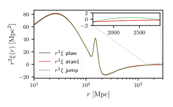
Figure 7: The predicted linear (3D) two-point functions for perturbations in the total cosmological matter density (conventionally denoted $\xi$ ) when the power-law primordial spectrum is modified by our best-fit deficit functions atan1 and jump. These fits are for the full Planck dataset.

Appendix A NUMCOSMO

In this appendix we briefly describe the numerical tools used in this work. These tools are part of the Numerical Cosmology library – NumCosmo Vitenti and Penna-Lima (2014). All codes described here are located in the project’s repository https://github.com/NumCosmo/NumCosmo and the library’s documentation is in https://numcosmo.github.io/. The library contains an independent implementation of several tools used in numerical cosmology, providing a complete toolkit to compute and analyze different cosmological observables. The observables were computed with the homogeneous and isotropic cosmological models objects (NcHICosmo*) and with the Boltzmann code using Class Blas et al. (2011); Lesgourgues (2011); Lesgourgues and Tram (2011) as back-end. Different precision files were used, all based on chi2pl0.01.pre (which was calibrated by the Class developers to provide a $10^{-3}$ error in $C_{\ell}$ at version 2.5.0). This precision file was modified to increase the number of points per decade to evaluate the PPS and to decrease the distance between interpolation points in $\ell$ (no interpolation for low-$\ell$ and increasing interpolation for high-$\ell$). This was necessary to capture the features added by the different deficit functions. We used three different precisions:

• The default class precision;

• The original file chi2pl0.01.pre with the addition – k_per_decade_primordial = 50.

• Same as MP but using –
  l_logstep = 1.02,
  q_linstep = 0.2.

After running the best-fit finder using these precisions, we found no relevant differences between MP and HP.

For the best-fit finders we used NumCosmo’s NcmFit object and the NLOpt (see Ref. Johnson (2014)) library as the minimization library back-end. We tested different numerical optimization algorithms. The most efficient and stable algorithms found were the Nelder-Mead Nelder and Mead (1965); Box (1965); Richardson and Kuester (1973) and Subplex Rowan (1990). The main advantage of these algorithms is that they do not require the objective function derivatives and have a better handling for discontinuous functions. The likelihood used is, in principle, a smooth function of the parameters $\theta$, although the computation of $C^{XY}_{\ell}$ introduces numerical errors in the evaluation of $L(D|\theta)$, which in turn can create artificial discontinuities at the error level. Accordingly, any optimization algorithm that depends on the smoothness of the likelihood (for example, some algorithms create a cubic approximation to the objective function or calculate an estimate of the derivative through finite differences) will find spurious maxima resulting from these small discontinuities (mainly on regions/direction where the likelihood is almost constant). In our fitting process we found that even the more appropriate algorithms terminate prematurely due to the artificial maxima. For this reason, we rerun the fitting process iteratively until the last two minima coincide within a 0.1% margin. This process was automated in the NcmFit.run_restart method.

We note a small difference between the parameter best-fit values using different precisions for the CMB anisotropies and/or accuracy for the minimization algorithm. The code used by Planck, CosmoMC Lewis et al. (2000); Lewis (2013), uses the BOBYQA Powell (2009) (Bound Optimization BY Quadratic Approximation) as the best-fit finder or even the point with smaller $-2\ln(L)$ value found during the MCMC exploration. We also tested these two methods. Both provide suboptimal minima with small differences in the best-fit parameters. The higher precision for the computation of the $C^{XX}_{\ell}$ and a more precise minimization algorithm resulted in best-fit parameters close to the ones previously obtained by the Planck team (with differences of the order of the precision for the $C^{XX}_{\ell}$, $\approx 10^{-3}$) but with larger differences in the values of the likelihood itself, that is, in the values of $\Gamma_{i}$ (with $\Delta\Gamma\approx 0.5$).

The MCMC algorithm used is identical to that used in Appendix D of Ref. Doux et al. (2018). Note however that, in our analysis, we did not use the profile likelihood for the PFI parameters: instead, we used a complete sample including all parameters. In Appendix E of Ref. Doux et al. (2018), one can find the description of all the diagnostics used to assert the convergence of the MCMC sampler.

Finally, we used the harmonic mean (see for context Weinberg (2012)) to estimate the evidence integral. In our implementation, our posterior sample was obtained from the MCMC to compute the integral

$$\left\langle g(\theta)\right\rangle=\int\mathrm{d}\theta g(\theta)P(\theta|\mathcal{M},D)\approx\frac{1}{N}\sum_{i}g(\theta_{i}),$$

where $\theta_{i}$ are the $N$ points in the posterior MCMC sample. Using Bayes theorem we have

$$\int\mathrm{d}\theta g(\theta)\frac{P(\theta|\mathcal{M})L(D|\theta,\mathcal{M})}{P(D|\mathcal{M})}\approx\frac{1}{N}\sum_{i}g(\theta_{i}),$$

where $L(D|\theta,\mathcal{M})$ is the likelihood and $P(\theta|\mathcal{M})$ the priors. We usually do not know the properly normalized likelihood $L(D|\theta,\mathcal{M})$, thus we define $L^{\prime}(D|\theta,\mathcal{M})\equiv N_{L}L(D|\theta,\mathcal{M})$, as the unnormalized likelihood (which is used in most cases for MCMC), and $N_{L}$ the normalization factor (which does not depend on any parameter), where the value of $P(\theta|\mathcal{M})L^{\prime}(D|\theta,\mathcal{M})$ was the one used by the MCMC sampler. For this reason we can choose

$$g(\theta)=\frac{F(\theta)}{P(\theta|\mathcal{M})L^{\prime}(D|\theta,\mathcal{M})},$$

to obtain

$$\frac{1}{N_{L}P(D|\mathcal{M})}\int\mathrm{d}\theta F(\theta)\approx\frac{1}{N}\sum_{i}\frac{F(\theta_{i})}{P(\theta_{i}|\mathcal{M})L^{\prime}(D|\theta_{i},\mathcal{M})}.$$

We then choose $F(\theta)$ to be a multivariate normal distribution with the mean and covariance equal to the estimates from the MCMC sample $\theta_{i}$. However, the support of $F(\theta)$ must be the same as that of $P(\theta|\mathcal{M},D)$ and therefore we normalize $F(\theta)$ in the same domain as $P(\theta|\mathcal{M},D)$ obtaining a truncated multivariate normal distribution. After the normalization we finally get our estimator for the reciprocal of $P(D|\mathcal{M})$ (modulo the irrelevant constant factor $N_{L}$):

$$\hat{\mathcal{Z}}\equiv\frac{1}{N_{L}P(D|\mathcal{M})}\approx\frac{1}{N}\sum_{i}\frac{F(\theta_{i})}{P(\theta_{i}|\mathcal{M})L^{\prime}(D|\theta_{i},\mathcal{M})}.$$

We computed the error in $\hat{\mathcal{Z}}$ using two methods. The first consists in splitting the sample $\theta_{i}$ into $M$ subsamples, computing $\hat{\mathcal{Z}}_{i}$ for each one, and from the results computing estimators for the mean and variance. The second method consists in bootstrapping $\theta_{i}$ (re-sampling with replacement), computing $\hat{\mathcal{Z}}_{i}$ for each bootstrap realization, and applying the usual mean and variance estimators. Both methods give numerically equivalent results.

Appendix B MODEL TABLES

In this Appendix, we discuss the information already present in Tables 1 to 12 but presented so as to allow an easy model-by-model comparison with respect to various datasets. Focusing on the favored models atan1 and jump, we briefly discuss the performance of each model with respect to all datasets used.

data-set	$k_{\mathrm{c}}^{-1}[\mathrm{Gpc}]$	$\lambda$	$\beta$	$\alpha$	$h$	$n_{\mathrm{s}}$	$\ln(10^{10}\mathcal{A}_{{}_{\mathrm{S}}})$	$\tau$	$\Gamma$	$\gamma$
Planck $TT$	$3.6$	$1$	$0$	$1$	$0.7$	$0.97$	$3.3$	$0.18$	$5.5$	$1.9$% ($2.4\sigma$) $[1]$
Planck $TT$+H0	$3$	$1$	$0$	$1$	$0.71$	$0.98$	$3.4$	$0.21$	$7.1$	$0.79$% ($2.7\sigma$) $[1]$
Planck $TT$+BAO	$3.5$	$1$	$0$	$1$	$0.69$	$0.97$	$3.3$	$0.18$	$4.6$	$3.2$% ($2.1\sigma$) $[1]$
Planck $TT$+H0+BAO	$3.9$	$1$	$0$	$1$	$0.69$	$0.97$	$3.3$	$0.17$	$5.6$	$1.8$% ($2.4\sigma$) $[1]$
Planck $TT$+lowP	$5.3$	$1$	$0$	$1$	$0.68$	$0.96$	$3.2$	$0.11$	$3.5$	$6.2$% ($1.9\sigma$) $[1]$
Planck $TT$+lowP+H0	$5.6$	$1$	$0$	$1$	$0.69$	$0.97$	$3.2$	$0.11$	$3.8$	$5.1$% ($1.9\sigma$) $[1]$
Planck $TT$+lowP+BAO	$5.3$	$1$	$0$	$1$	$0.68$	$0.96$	$3.2$	$0.11$	$3.5$	$6$% ($1.9\sigma$) $[1]$
Planck $TT$+lowP+H0+BAO	$5.7$	$1$	$0$	$1$	$0.69$	$0.97$	$3.1$	$0.1$	$3.9$	$4.9$% ($2\sigma$) $[1]$
Planck $TT$, $TE$, $EE$+lowP	$6.5$	$1$	$0$	$1$	$0.67$	$0.96$	$3.1$	$0.094$	$3.4$	$6.7$% ($1.8\sigma$) $[1]$
Planck $TT$, $TE$, $EE$+lowP+H0	$7.3$	$1$	$0$	$1$	$0.68$	$0.96$	$3.1$	$0.096$	$3.2$	$7.4$% ($1.8\sigma$) $[1]$
Planck $TT$, $TE$, $EE$+lowP+BAO	$7$	$1$	$0$	$1$	$0.68$	$0.96$	$3.1$	$0.095$	$3.2$	$7.4$% ($1.8\sigma$) $[1]$
Planck $TT$, $TE$, $EE$+lowP+H0+BAO	$6.6$	$1$	$0$	$1$	$0.68$	$0.96$	$3.1$	$0.099$	$3.2$	$7.1$% ($1.8\sigma$) $[1]$

Table 13: Excerpt from Tables 1 to 12 selecting the results for atan1, see Table 1 for more details.

B.1 Inverse tangent model: atan1

The atan model given by Eq. (8) provides a very smooth deficit correction to the fiducial PPS. In fact, the parameter $k_{\mathrm{c}}$ is not really a characteristic scale in this case, as can be seen by the following example: setting $\beta=0$, $\alpha=1$ and $\lambda=1$, one obtains the following values for $X_{\xi}\equiv k/k_{\mathrm{c}}$

$$X_{1\%}=0.01,$$ (27)

$$X_{5\%}=0.07,$$ (28)

$$X_{20\%}=0.33,$$ (29)

$$X_{80\%}=4.3,$$ (30)

$$X_{95\%}=19,$$ (31)

$$X_{99\%}=99,$$ (32)

where the index indicates the amplitude reduction compared to the fiducial PPS.

In words, Eqs. (27) to (32) show that $\xi_{\mathrm{neq}}$ starts decreasing the amplitude of the PPS already for, say, $X_{99\%}=99$, which implies $k_{99\%}^{-1}=k_{\mathrm{c}}^{-1}/99$. Therefore, for a fit with $k_{\mathrm{c}}^{-1}\approx 3.5\;\mathrm{Gpc}$ say, the modification starts around $\approx 35\;\mathrm{Mpc}$, the power drop reaching 20% for $k_{80\%}^{-1}=k_{\mathrm{c}}^{-1}/4.3\approx 914\;\mathrm{Mpc}$. Moreover, the total deficit window can be very wide: in the case at hand, one has $X_{99\%}/X_{1\%}\approx 10^{4}$, so that $k$ varies over four orders of magnitude within the deficit window. A more conservative window, from 20% to 80% say, leads to $X_{80\%}/X_{20\%}\approx 13$, which still requires a full order of magnitude variation of $k$. When $\beta\neq 0$, the only difference is that the deficit window ends, roughly, when $X<X_{\beta}$.

The most significant parametrization for the atan model is the special case atan1; Table 13 summarizes our findings for this model. We observe that adding polarization data has an effect opposite to what we found for bpl, with the value of $k^{-1}_{\mathrm{c}}$ getting larger as we include more polarization datasets (independently of the other datasets used, H0 and/or BAO). This occurs because the deficit actually worsens the polarization fit, so the effect needs be reduced in order to improve the temperature fit without spoiling the polarization fit. Since this model has a single parameter, the only way to achieve that is by pushing this parameter to a larger scale. Similarly to bpl, when using temperature data only, the larger deficit is compensated for by a 15%-20% increase in the spectrum amplitude.

Although this model seems to provide fits which are better than for the fiducial case, in some cases with an improvement close to $2.5\sigma$, these fits are actually not reliable because they are unstable with respect to the parameter values obtained. Indeed, when polarization data are added, the parameters change abruptly and, moreover, the significance is reduced, as expected for a statistical fluctuation. Finally, including all datasets, we obtain a marginal $1.8\sigma$ significance for a smooth and broad deficit at very large scales.

data-set	$k_{\mathrm{c}}^{-1}[\mathrm{Gpc}]$	$\lambda$	$\beta$	$\alpha$	$h$	$n_{\mathrm{s}}$	$\ln(10^{10}\mathcal{A}_{{}_{\mathrm{S}}})$	$\tau$	$\Gamma$	$\gamma$
Planck $TT$	$0.36$	–	$0.78$	–	$0.69$	$0.98$	$3.3$	$0.17$	$6.8$	$3.4$% ($2.1\sigma$) $[2]$
Planck $TT$+H0	$0.35$	–	$0.76$	–	$0.7$	$0.99$	$3.3$	$0.2$	$7.2$	$2.8$% ($2.2\sigma$) $[2]$
Planck $TT$+BAO	$0.36$	–	$0.79$	–	$0.68$	$0.97$	$3.3$	$0.16$	$6.8$	$3.4$% ($2.1\sigma$) $[2]$
Planck $TT$+H0+BAO	$0.35$	–	$0.77$	–	$0.69$	$0.98$	$3.3$	$0.18$	$6.7$	$3.5$% ($2.1\sigma$) $[2]$
Planck $TT$+lowP	$0.37$	–	$0.81$	–	$0.68$	$0.97$	$3.1$	$0.1$	$5.1$	$8$% ($1.8\sigma$) $[2]$
Planck $TT$+lowP+H0	$0.37$	–	$0.81$	–	$0.69$	$0.97$	$3.2$	$0.12$	$4.6$	$10$% ($1.6\sigma$) $[2]$
Planck $TT$+lowP+BAO	$0.37$	–	$0.8$	–	$0.68$	$0.97$	$3.2$	$0.12$	$4.3$	$11$% ($1.6\sigma$) $[2]$
Planck $TT$+lowP+H0+BAO	$0.37$	–	$0.81$	–	$0.69$	$0.97$	$3.2$	$0.12$	$4.8$	$9.2$% ($1.7\sigma$) $[2]$
Planck $TT$, $TE$, $EE$+lowP	$0.38$	–	$0.82$	–	$0.67$	$0.96$	$3.1$	$0.093$	$5.8$	$5.5$% ($1.9\sigma$) $[2]$
Planck $TT$, $TE$, $EE$+lowP+H0	$0.39$	–	$0.82$	–	$0.68$	$0.97$	$3.1$	$0.095$	$5.3$	$7.1$% ($1.8\sigma$) $[2]$
Planck $TT$, $TE$, $EE$+lowP+BAO	$0.38$	–	$0.83$	–	$0.68$	$0.97$	$3.1$	$0.093$	$5.3$	$7.1$% ($1.8\sigma$) $[2]$
Planck $TT$, $TE$, $EE$+lowP+H0+BAO	$0.38$	–	$0.83$	–	$0.68$	$0.97$	$3.1$	$0.095$	$5.1$	$7.7$% ($1.8\sigma$) $[2]$

Table 14: Excerpt from Tables 1 to 12 selecting the results for jump, see Table 1 for more details.

B.2 Sharp deficit model: jump

The results for this model are summarized in Table 14. We observe that the parameter values are now consistent across all datasets, although the significance remains marginal and resembles those for atan1 and expc2. In the case of jump, however, all datasets point in the same general direction and parameter values that provide a good fit for one dataset also provide a good fit for the others. This means that, to have a hope of measuring an effect using the full range of datasets, we need to consider the jump model.

References

- Peter and Uzan (2013) P. Peter and J.-P. Uzan, Primordial Cosmology, Oxford Graduate Texts (Oxford University Press, 2013), ISBN 9780199665150, 9780199209910.
- Schwarz et al. (2016) D. J. Schwarz, C. J. Copi, D. Huterer, and G. D. Starkman, Class. Quant. Grav. 33, 184001 (2016), eprint 1510.07929.
- Chluba et al. (2015) J. Chluba, J. Hamann, and S. P. Patil, Int. J. Mod. Phys. D24, 1530023 (2015), eprint 1505.01834.
- Planck Collaboration et al. (2014a) Planck Collaboration, P. A. R. Ade, N. Aghanim, C. Armitage-Caplan, M. Arnaud, M. Ashdown, F. Atrio-Barandela, J. Aumont, C. Baccigalupi, A. J. Banday, et al., Astron. Astrophys. 571, A22 (2014a), eprint 1303.5082.
- Ade et al. (2016) P. A. R. Ade et al. (Planck), Astron. Astrophys. 594, A20 (2016), eprint 1502.02114.
- Planck Collaboration et al. (2018) Planck Collaboration, Y. Akrami, F. Arroja, M. Ashdown, J. Aumont, C. Baccigalupi, M. Ballardini, A. J. Banday, R. B. Barreiro, N. Bartolo, et al., arXiv e-prints arXiv:1807.06211 (2018), eprint 1807.06211.
- Bennett et al. (1996) C. L. Bennett, A. J. Banday, K. M. Gorski, G. Hinshaw, P. Jackson, P. Keegstra, A. Kogut, G. F. Smoot, D. T. Wilkinson, and E. L. Wright, Astrophys. J. 464, L1 (1996), eprint astro-ph/9601067.
- Bennett et al. (2003) C. L. Bennett, M. Halpern, G. Hinshaw, N. Jarosik, A. Kogut, M. Limon, S. S. Meyer, L. Page, D. N. Spergel, G. S. Tucker, et al., Astrophys. J. Suppl. Ser. 148, 1 (2003), eprint astro-ph/0302207.
- Spergel et al. (2003) D. N. Spergel, L. Verde, H. V. Peiris, E. Komatsu, M. R. Nolta, C. L. Bennett, M. Halpern, G. Hinshaw, N. Jarosik, A. Kogut, et al., Astrophys. J. Suppl. Ser. 148, 175 (2003), eprint astro-ph/0302209.
- Contaldi et al. (2003) C. R. Contaldi, M. Peloso, L. Kofman, and A. Linde, J. Cosmol. Astropart. Phys 2003, 002 (2003), eprint astro-ph/0303636.
- Bridle et al. (2003) S. L. Bridle, A. M. Lewis, J. Weller, and G. Efstathiou, Mon. Not. R. Astron. Soc. 342, L72 (2003), eprint astro-ph/0302306.
- Efstathiou (2003a) G. Efstathiou, Mon. Not. R. Astron. Soc. 343, L95 (2003a), eprint astro-ph/0303127.
- Efstathiou (2003b) G. Efstathiou, Mon. Not. R. Astron. Soc. 346, L26 (2003b), eprint astro-ph/0306431.
- Kawasaki and Takahashi (2003) M. Kawasaki and F. Takahashi, Phys. Lett. B 570, 151 (2003), eprint hep-ph/0305319.
- de Oliveira-Costa et al. (2004) A. de Oliveira-Costa, M. Tegmark, M. Zaldarriaga, and A. Hamilton, Phys. Rev. D 69, 063516 (2004), eprint astro-ph/0307282.
- Martin and Ringeval (2004) J. Martin and C. Ringeval, Phys. Rev. D 69, 083515 (2004), eprint astro-ph/0310382.
- Park and Ratra (2018) C.-G. Park and B. Ratra, Astrophys. J. 868, 83 (2018), eprint 1807.07421.
- Muir et al. (2018) J. Muir, S. Adhikari, and D. Huterer, Phys. Rev. D98, 023521 (2018), eprint 1806.02354.
- Bennett et al. (2011) C. L. Bennett, R. S. Hill, G. Hinshaw, D. Larson, K. M. Smith, J. Dunkley, B. Gold, M. Halpern, N. Jarosik, A. Kogut, et al., Astrophys. J. Suppl. Ser. 192, 17 (2011), eprint 1001.4758.
- Riess et al. (2016) A. G. Riess, L. M. Macri, S. L. Hoffmann, D. Scolnic, S. Casertano, A. V. Filippenko, B. E. Tucker, M. J. Reid, D. O. Jones, J. M. Silverman, et al., Astrophys. J. 826, 56 (2016), eprint 1604.01424.
- Obied et al. (2017) G. Obied, C. Dvorkin, C. Heinrich, W. Hu, and V. Miranda, Phys. Rev. D 96, 083526 (2017), eprint 1706.09412.
- Wang and Ng (2008) I.-C. Wang and K.-W. Ng, Phys. Rev. D77, 083501 (2008), eprint 0704.2095.
- Colin and Valentini (2015) S. Colin and A. Valentini, Phys. Rev. D92, 043520 (2015), eprint 1407.8262.
- Colin and Valentini (2016) S. Colin and A. Valentini, Int. J. Mod. Phys. D25, 1650068 (2016), eprint 1510.03508.
- Colin and Valentini (2013) S. Colin and A. Valentini, Phys. Rev. D88, 103515 (2013), eprint 1306.1579.
- Valentini (2010) A. Valentini, Phys. Rev. D82, 063513 (2010), eprint 0805.0163.
- Jeffreys (1998) H. Jeffreys, The Theory of Probability, Oxford Classic Texts in the Physical Sciences (OUP Oxford, 1998), ISBN 9780191589676.
- Hazra et al. (2013) D. K. Hazra, A. Shafieloo, and G. F. Smoot, JCAP 1312, 035 (2013), eprint 1310.3038.
- Peter and Pinto-Neto (2008) P. Peter and N. Pinto-Neto, Phys. Rev. D78, 063506 (2008), eprint 0809.2022.
- Battefeld and Peter (2015) D. Battefeld and P. Peter, Phys. Rep. 571, 1 (2015), eprint 1406.2790.
- Brandenberger and Peter (2017) R. Brandenberger and P. Peter, Found. Phys. 47, 797 (2017), eprint 1603.05834.
- Bacalhau et al. (2018) A. P. Bacalhau, N. Pinto-Neto, and S. r. D. P. Vitenti, Phys. Rev. D 97, 083517 (2018), eprint 1706.08830.
- Lewis et al. (2000) A. Lewis, A. Challinor, and A. Lasenby, Astrophys. J. 538, 473 (2000), eprint astro-ph/9911177.
- Lewis (2013) A. Lewis, Phys. Rev. D 87, 103529 (2013).
- Goodman and Weare (2010) J. Goodman and J. Weare, CAMCoS 5, 65 (2010).
- Foreman-Mackey et al. (2013) D. Foreman-Mackey, D. W. Hogg, D. Lang, and J. Goodman, Publications of the Astronomical Society of the Pacific 125, 306 (2013).
- Planck Collaboration et al. (2014b) Planck Collaboration, P. A. R. Ade, N. Aghanim, C. Armitage-Caplan, M. Arnaud, M. Ashdown, F. Atrio-Barandela, J. Aumont, C. Baccigalupi, A. J. Banday, et al., Astron. Astrophys. 571, A16 (2014b), eprint 1303.5076.
- Planck Collaboration et al. (2015) Planck Collaboration, P. A. R. Ade, N. Aghanim, M. Arnaud, M. Ashdown, J. Aumont, C. Baccigalupi, A. J. Banday, R. B. Barreiro, J. G. Bartlett, et al., Astron. Astrophys. 594, A13 (2015), eprint 1502.01589.
- Planck Collaboration et al. (2016) Planck Collaboration, N. Aghanim, M. Arnaud, M. Ashdown, J. Aumont, C. Baccigalupi, A. J. Band ay, R. B. Barreiro, J. G. Bartlett, N. Bartolo, et al., Astron. Astrophys. 594, A11 (2016), eprint 1507.02704.
- Beutler et al. (2011) F. Beutler, C. Blake, M. Colless, D. H. Jones, L. Staveley-Smith, L. Campbell, Q. Parker, W. Saunders, and F. Watson, Mon. Not. R. Astron. Soc. 416, 3017 (2011), eprint 1106.3366.
- Ross et al. (2015) A. J. Ross, L. Samushia, C. Howlett, W. J. Percival, A. Burden, and M. Manera, Mon. Not. Roy. Astron. Soc. 449, 835 (2015), eprint 1409.3242.
- Alam et al. (2017) S. Alam, M. Ata, S. Bailey, F. Beutler, D. Bizyaev, J. A. Blazek, A. S. Bolton, J. R. Brownstein, A. Burden, C.-H. Chuang, et al., Mon. Not. R. Astron. Soc. 470, 2617 (2017), eprint 1607.03155v1.
- Ata et al. (2018) M. Ata, F. Baumgarten, J. Bautista, F. Beutler, D. Bizyaev, M. R. Blanton, J. A. Blazek, A. S. Bolton, J. Brinkmann, J. R. Brownstein, et al., Mon. Not. R. Astron. Soc. 473, 4773 (2018), eprint 1705.06373.
- Delubac et al. (2015) T. Delubac, J. E. Bautista, N. G. Busca, J. Rich, D. Kirkby, S. Bailey, A. Font-Ribera, A. Slosar, K.-G. Lee, M. M. Pieri, et al., Astron. Astrophys. 574, A59 (2015), eprint 1404.1801.
- Font-Ribera et al. (2014) A. Font-Ribera, D. Kirkby, N. Busca, J. Miralda-Escudé, N. P. Ross, A. Slosar, J. Rich, É. Aubourg, S. Bailey, V. Bhardwaj, et al., J. Cosmol. Astropart. Phys. 5, 027 (2014), eprint 1311.1767.
- Craig (1984) H. Craig, Introduction to Mathematical Statistics (Prentice Hall, 1984).
- Hoel (2003) P. G. Hoel, Introduction to Mathematical Statistics (John Wiley & Sons, 2003).
- van der Vaart (2000) A. van der Vaart, Asymptotic Statistics, Cambridge Series in Statistical and Probabilistic Mathematics (Cambridge University Press, 2000), ISBN 9780521784504.
- Blas et al. (2011) D. Blas, J. Lesgourgues, and T. Tram, J. Cosmol. Astropart. Phys. 2011, 034 (2011).
- Lesgourgues (2011) J. Lesgourgues, ArXiv e-prints (2011), eprint 1104.2934.
- Lesgourgues and Tram (2011) J. Lesgourgues and T. Tram, J. Cosmol. Astropart. Phys. 9, 032 (2011), eprint 1104.2935.
- Trotta (2007) R. Trotta, Mon. Not. R. Astron. Soc. 378, 72 (2007), eprint astro-ph/0504022.
- Kandhadai and Valentini (in preparation) A. Kandhadai and A. Valentini (in preparation).
- Valentini (2015) A. Valentini (2015), eprint 1510.02523.
- Laurent et al. (2016) P. Laurent et al., JCAP 1611, 060 (2016), eprint 1602.09010.
- Ntelis et al. (2017) P. Ntelis et al., JCAP 1706, 019 (2017), eprint 1702.02159.
- Laureijs et al. (2011) R. Laureijs, J. Amiaux, S. Arduini, J. L. Auguères, J. Brinchmann, R. Cole, M. Cropper, C. Dabin, L. Duvet, A. Ealet, et al., arXiv e-prints arXiv:1110.3193 (2011), eprint 1110.3193.
- Vitenti and Penna-Lima (2014) S. D. P. Vitenti and M. Penna-Lima, Numerical cosmology – NumCosmo, Astrophysics Source Code Library (2014), eprint 1408.013, URL https://github.com/NumCosmo/NumCosmo.
- Johnson (2014) S. G. Johnson, The nlopt nonlinear-optimization package (2014).
- Nelder and Mead (1965) J. A. Nelder and R. Mead, Comput. J. 7, 308 (1965).
- Box (1965) M. J. Box, Comput. J. 8, 42 (1965).
- Richardson and Kuester (1973) J. A. Richardson and J. L. Kuester, Commun. ACM 16, 487 (1973), ISSN 0001-0782.
- Rowan (1990) T. H. Rowan, Tech. Rep., University of Texas at Austin (1990).
- Powell (2009) M. J. D. Powell (2009), URL http://www.damtp.cam.ac.uk/user/na/NA_papers/NA2009_06.pdf.
- Doux et al. (2018) C. Doux, M. Penna-Lima, S. D. P. Vitenti, J. Tréguer, E. Aubourg, and K. Ganga, Mon. Not. R. Astron. Soc. 480, 5386 (2018), eprint 1706.04583, URL http://adsabs.harvard.edu/abs/2018MNRAS.480.5386D.
- Weinberg (2012) M. D. Weinberg, Bayesian Anal. 7, 737 (2012), URL https://doi.org/10.1214/12-BA725.