Internal Gravity Waves in the Magnetized Solar Atmosphere.
II. Energy Transport

G. Vigeesh¹¹affiliationmark: , M. Roth¹¹affiliationmark: , O. Steiner¹¹affiliationmark: ²²affiliationmark: , and J. Jackiewicz³³affiliationmark: ¹¹affiliationmark: Leibniz-Institut für Sonnenphysik (KIS), Schöneckstrasse 6, 79104 Freiburg, Germany
²²affiliationmark: Istituto Ricerche Solari Locarno (IRSOL), via Patocchi 57-Prato Pernice, 6605 Locarno-Monti, Switzerland
³³affiliationmark: New Mexico State University, Department of Astronomy, P.O. Box 30001, MSC 4500, Las Cruces, NM 88003, USA vigeesh@leibniz-kis.de

Abstract

In this second paper of the series on internal gravity waves (IGWs), we present a study of the generation and propagation of IGWs in a model solar atmosphere with diverse magnetic conditions. A magnetic field free, and three magnetic models that start with an initial, vertical, homogeneous field of 10 G, 50 G, and 100 G magnetic flux density, are simulated using the CO⁵BOLD code. We find that the IGWs are generated in similar manner in all four models in spite of the differences in the magnetic environment. The mechanical energy carried by IGWs is significantly larger than that of the acoustic waves in the lower part of the atmosphere, making them an important component of the total wave energy budget. The mechanical energy flux (10⁶–10³ W m^-2) is few orders of magnitude larger than the Poynting flux (10³–10¹ W m^-2). The Poynting fluxes show a downward component in the frequency range corresponding to the IGWs, which confirm that these waves do not propagate upwards in the atmosphere when the fields are predominantly vertical and strong. We conclude that, in the upper photosphere, the propagation properties of IGWs depend on the average magnetic field strength and therefore these waves can be potential candidate for magnetic field diagnostics of these layers. However, their subsequent coupling to Alfvénic waves are unlikely in a magnetic environment permeated with predominantly vertical fields and therefore they may not directly or indirectly contribute to the heating of layers above plasma- $\beta$ less than 1.

magnetohydrodynamics (MHD) — Sun: atmosphere — Sun: granulation — Sun: magnetic fields — Sun: photosphere — waves

^†^†software: CO⁵BOLD (2012JCoPh.231..919F), NumPy (walt2011numpy), SciPy (jones2001scipy), Matplotlib (2007CSE.....9...90H), Astropy (2013A&A...558A..33A), Cython (behnel2010cython)

1 Introduction

Atmospheric waves are part and parcel of any gravitating body that has a gaseous envelope. Whether it be terrestrial or other planetary atmospheres, or the solar atmosphere—a plethora of waves are found in them that are responsible for energy and momentum transport across its different layers. In the case of the Sun, these waves play an important role in the overall dynamics of the solar atmosphere and help to connect its lower layer—a region where a majority of the waves supposedly originate, with its upper layers.

Internal gravity waves (IGWs) are archetype of atmospheric waves with buoyancy acting as their main driving mechanism (2001wafl.book.....L; sutherland2010). When compressibility effects are also taken into account, a combination of IGWs and sound waves are supported in the atmosphere, resulting in more general acoustic-gravity spectra. In the case of a magnetized atmosphere, the magnetic fields introduces yet another restoring effect in the form of the Lorentz force leading to a more complex system of coupled wave phenomena collectively referred to as magneto-acoustic-gravity or MAG waves. Apart from the gaseous envelope that surrounds a stellar object, these waves can also occur in the radiative interiors of cool-stars, where the criterion for the existence of such waves are equally satisfied.

In the solar atmosphere, IGWs have been observed and are thought to contribute to the overall energy budget (2008ApJ...681L.125S). IGWs are also searched for in the deep radiative interior of the Sun where they form standing waves called $g$ -modes (see 2010A&ARv..18..197A, for a review, or 2017A&A...604A..40F, for more recent work). Particularly, the latter have been subject of active research due to the distinctive role they play in these stable regions. They are invoked to explain the rigid-body rotation of the solar interior as a result of angular momentum redistribution by them (1993A&A...279..431S; 1997ApJ...475L.143K; 1997A&A...322..320Z; 2002ApJ...574L.175T; 2008MNRAS.387..616R). In addition to that, their role in the mixing of chemical species and the Lithium depletion are still being debated (2017ApJ...848L...1R).

The effect of magnetic fields on the propagation of IGW has also received attention (1998ApJ...498L.169B). The existence of a sufficiently strong magnetic field (10⁵G) in the interiors of stars may restrict certain wavenumbers from propagating and can even alter the location of critical layers typically associated with strong shear flow that affects IGWs. IGWs propagating in the radiative interiors of stars can also interact with the large-scale magnetic field, if the IGW frequency is approximately equal to that of the Alfvén frequency, resulting in reflection of the waves and consequently affecting the angular momentum transport (2010MNRAS.401..191R; 2011MNRAS.410..946R). It also was shown that a critical field strength exist that can result in the conversion of IGWs into other magneto-acoustic waves, which can be used for asteroseismic measurements of the internal magnetic fields in red giant stars (2015Sci...350..423F; 2017MNRAS.466.2181L).

In the same spirit, the solar atmosphere is equally interesting as it not only harbors magnetic field on every possible scale but also supports IGWs. The solar atmosphere is one case where the effect of magnetic fields on IGWs may be of significance and observable. More recent works have looked at propagating and standing IGWs in a gravitationally stratified medium in the presence of a background vertical magnetic field (2016ApJ...828...88H) and studies of the full MAG spectra has also been carried out (2013SoPh..283..383M; 2016ApJ...822..116M).

The generation mechanism of IGWs in the solar, and in general in the stellar case (both in the interior as well as the atmosphere) mainly fall under the category of convection driving mechanism (1990ApJ...363..694G). This is in sharp contrast with the variety of different mechanisms possible in the terrestrial case (e.g. 2003RvGeo..41.1003F, and references therein), which also includes orographic generation by winds passing over mountain terrain. Convective overshooting at the location of a convective/stable interface (1986ApJ...311..563H; 1990ApJ...363..694G; 2005MNRAS.364.1135R; 2013MNRAS.430.2363L; 2010JFM...648..405A; 2014A&A...565A..42A; 2015A&A...581A.112A; 2016A&A...588A.122P; 2017A&A...605A..31P) is thought to be how IGWs are generated in the solar atmosphere. This has been confirmed by reported observations of IGWs in the solar atmosphere by several authors (1991A&A...252..827K; 2003A&A...407..735R; 2008ApJ...681L.125S; 2008MNRAS.390L..83S; 2009ASPC..415...95S; 2011A&A...532A.111K; 2014SoPh..289.3457N).

2017ApJ...835..148V looked at IGWs generated in model solar atmospheres and investigated the effect of magnetic fields on their propagation. We used state-of-the-art three-dimensional numerical simulations to study atmospheric IGWs in the presence of spatially and temporally evolving magnetic fields with waves naturally excited in them by convection. The work was a significant extension to the linear analysis that was carried out by 1982ApJ...263..386M; 1981ApJ...249..349M. We considered two models, a non-magnetic and a magnetic model, and studied the differences in wave spectra emerging from the two atmospheres. Internal waves are generated in both models and overcome the strong radiative damping in the lower photosphere to propagate into the higher layers. The presence of magnetic fields show a strong influence on these waves as they propagate higher up in the atmosphere. We concluded that the internal waves in the quiet Sun likely undergo mode coupling to slow magneto-acoustic waves as described by 2011MNRAS.417.1162N; 2010MNRAS.402..386N and are thereby mostly reflected back into the atmosphere.

The mode coupling scenario was further confirmed by the fact that the mechanical flux showed a mixed upward and downward component in the internal gravity wave regime for the magnetic case in the higher layers while there was only an upward component in the non-magnetic case. As the magnetic fields in this model was predominantly vertical, conversion to Alfvén waves was speculated to be highly unlikely. Because of the lack of additional magnetic models to confirm this scenario, a study of this was not pursued in Paper I. We also speculated that the strong suppression of IGWs within magnetic flux-concentration observed by 2008ApJ...681L.125S may be due to non-linear wave breaking as a result of vortex flows that are ubiquitously present in these regions (2012Natur.486..505W).

Our analysis, presented in Paper I, shows that a considerable amount of internal wave flux is produced in the near surface layers and that these waves can couple with other magneto-atmospheric waves. Hence, it is important to fully understand the transfer of energy from these waves to other waves in the atmosphere of the Sun in order to account for the complete energy sources related to wave motion. The generation of internal waves and how magnetic fields influence their generation in a realistic solar model atmosphere is of great interest. Whether these waves carry sufficient energy to balance the overall energy budget of the upper atmosphere and how the presence of magnetic field affect the energy transport is still unclear. To this end, we present here a study of IGWs in dynamic model solar atmospheres of different magnetic flux density and look at gravity wave excitation and propagation in them. We are interested in a quantitative estimate and comparison of the energy flux associated with these waves in diverse magnetic environments that are representative of different regions on the Sun with magnetic flux densities that resemble regions of the Sun ranging from the quiet Sun to plages.

The paper is structured as follows: In Section 2, we present the numerical setup and describe the properties of the different models. In Section 3, we briefly describe the spectral analysis of the 3D simulation which was already presented in Paper I. Section 4 presents the results of the spectral analysis and looks at the differences in the the phase and energy flux spectra from the different models. Section 5, we discuss similarities in the generation and differences in the energy transport by the waves in these models. The conclusion of the paper is given in Section 6.

2 Numerical Models

Table 1: Numerical setup and physical properties of the four simulated models.

	Sun-v0	Sun-v10	Sun-v50	Sun-v100
	(SVGd3r05bn0cp1p¹¹1 Original identifier)	(SVGd3r12bv1cp1p)	(SVGd3r09bv5cp1p)	(SVGd3r13bvCcp1p)
Snapshot cadence	30 s
Duration of simulation	4 hrs
Computational grid	480 $\times$ 480 $\times$ 120
Domain size	38.4 $\times$ 38.4 $\times$ 2.8 Mm³
Computational cell size	80 $\times$ 80 $\times$ (50-20)²²2 The vertical cell size varies from 50 km in the lower part of the computational domain down to 20 km in the upper atmosphere. km³
Numerical scheme	HLL-MHD
Reconstruction scheme	FRweno
Initial field, $B_{z}$ (uniform)	0 G	10 G	50 G	100 G
Temperature, $T_{\rm eff}$	5759.2 $\pm$ 3.7 K	5760.1 $\pm$ 3.6 K	5766.8 $\pm$ 3.4 K	5775.0 $\pm$ 3.3 K
Intensity contrast, $\delta I_{\rm bol}^{\rm rms}$	15.38 $\pm$ 0.09 %	15.27 $\pm$ 0.10 %	14.82 $\pm$ 0.10 %	14.32 $\pm$ 0.10 %

We use numerical simulations to mimic the dynamics of a small region near the surface of the Sun from where the waves likely emanate. The simulated domain is a thin slab that encompasses a small portion of the convective interior as well as the radiative atmospheric layer of the star. We carry out the full forward modeling of this near-surface solar magnetoconvection using the CO⁵BOLD³³3 CO5BOLD (nicknamed COBOLD), is the short form of “COnservative COde for the COmputation of COmpressible COnvection in a BOx of L Dimensions with l=2,3”. In this work we use l=3. code (version 002.02.2012.11.05e; 2012JCoPh.231..919F) in its box-in-a-star setup. The code solves the time-dependent non-linear magnetohydrodynamics (MHD) equations in a Cartesian box with an external gravity field and taking non-grey radiative transfer into account.

The radiative-MHD code, CO⁵BOLD, has been extensively used for various applications that model the solar, stellar and sub-stellar atmospheres. This includes, but is not limited to, chromospheres of red giants (2017A&A...606A..26W), AGB stars (2017A&A...600A.137F) to magnetic field effects in white dwarfs (2015ApJ...812...19T) and small-scale magnetism in main sequence stellar atmospheres (2018A&A...614A..78S) to brown dwarfs (2013MmSAI..84.1070F). CO⁵BOLD has proven to be a valuable tool in studies including the determination of Oxygen and Lithium abundance in cool stars (2008A&A...488.1031C; 2017A&A...604A..44M). It has also been used for local helioseismology studies as well as to study waves in the solar atmosphere (2007AN....328..323S; 2008ApJ...681L.125S; 2012A&A...542L..30N; 2011ApJ...730L..24K; 2016ApJ...827....7K). The code allows for the continuous simulation of solar- and stellar convection for long time periods making it a convenient tool to investigate waves that naturally occur at the interface between a convective and stable environment.

In the first part of this work (Paper I), we discussed two different simulations, viz. a hydrodynamic and a magnetohydrodynamic run that were carried out using the CO⁵BOLD code. We studied the differences in wave spectra emerging from the two physically disparate surface convection regimes, one without and the other with magnetic field. Apart from the differences in the non-linear equations solved, the other notable difference between the two runs were in the numerical solvers that were used. The hydrodynamic run was carried out with a Roe solver and the MHD run used a HLL (Harten, Lax & van Leer) solver. It was seen that the HLL-MHD numerical solver is more diffusive compared to the Roe solver which resulted in a significant difference in the size of granules between the hydrodynamic and magnetohydrodynamic simulated models. Despite these differences, the overall wave spectra that originated from the surface convection of both models were found to be the same.

In this work, we carry out a set of four new simulations of the solar convection that includes a non-magnetic and three magnetic cases, as explained later. In order to make a more precise comparison, we now use the same solver (HLL-MHD; 2005ESASP.596E..65S; 2013MSAIS..24..100S) for all runs in this work. Additionally, instead of using the PP (Piecewise Parabolic) reconstruction scheme as in the previous study (Paper I), we now use the more robust FRweno scheme (2013MSAIS..24...26F), which is a combination of PP and WENO (weighted essentially non-oscillatory) reconstruction methods. The FRweno reconstruction scheme is applied in the horizontal coordinates, but switches to the van Leer scheme in the vertical coordinate due to the non-equidistant nature of the computational grid in that direction.

All four models start with a three-dimensional (3D) state taken from a relaxed convection simulation without magnetic field carried out using the CO⁵BOLD code. The computational domain is 38.4 $\times$ 38.4 $\times$ 2.8 Mm³, discretized on 480 $\times$ 480 $\times$ 120 grid cells, extending $\sim$ 1.5 Mm below the mean Rosseland optical depth $\tau_{R}=1$ . The atmosphere wherein the waves propagate extends over a height of $\sim$ 1.3 Mm above this level. The non-magnetic run (Sun-v0) is computed by setting the initial magnetic flux density to zero. The three magnetic runs, viz, Sun-v10, Sun-v50, and Sun-v100 are computed by embedding the initial model with a uniform vertical field of 10 G, 50 G, and 100 G, respectively, in the entire domain. All the four models are advanced for a timespan of 60 minutes to adjust to the new solver and to redistribute the imposed magnetic fields. Starting with this snapshot as the new initial model for the four runs, we advance the models for 4 hours taking a 3D snapshot every 30 seconds. A summary of the simulation setup is shown in Table 1.

The boundary conditions that we use in this new set of runs are similar to the ones that were used in Paper I. As is normally the case with side boundaries for studying waves, we use periodic boundary conditions on the velocity, radiation and the magnetic field. Periodic boundary conditions have the least interference with waves that propagate within the computational domain. The top boundary is open for fluid flow and outward radiation and the density is set to drop exponentially into the ghost cells. The bottom boundary is also open with a condition on the specific entropy of the in-flowing material as described in Paper I. The magnetic fields are forced to be vertical at the top and bottom boundary by setting the vertical component of the magnetic field constant and the transverse component zero across the boundary into the ghost cells.

An equation of state that adequately describes the solar plasma including partial ionization effects is provided in a tabulated form. The radiative transfer proceeds via a opacity binning method, with the help of five opacity groups, adapted from the MARCS stellar atmosphere package (2008A&A...486..951G). For the radiative transfer we use long-characteristics along a set of 8 rays. An Alfvén speed-limiter with a maximum Alfvén speed of 40 km s^-1 is used to make the time-stepping within computationally feasible limits. The effect of this is not significant on the waves that we study and will be discussed later in the appropriate section.

3 Analysis

We carry out a spectral analysis of the 3D simulations by Fourier transforming the physical quantities in both space and time to identify and seperate IGW from other types of waves present in the domain. The fact that we are not dealing with a uniform medium (as the quantities vary with height) is for the present study ignored, treating the medium as locally homogeneous in the horizontal direction. All the physical variables are decomposed into their Fourier components in the horizontal directions and in time for each grid point in the $z$ -direction. Although we use only 4 hour long duration of simulation, it gives us adequate spectral resolution to identify waves. A tapered cosine window is used for apodization in the temporal direction to account for the abrupt start and end of selected segment. The spatial direction is not apodized as we have used a periodic boundary condition for the lateral sides in the simulation. The Fourier synthesis is carried out using the Fast Fourier Transform (FFT) algorithm and the derived Fourier components are then represented on a $k_{h}-\omega$ diagram for each height level by azimuthally averaging over the $k_{x}-k_{y}$ plane. A detailed description of the analysis is given in Paper I for further reference.

4 Results

4.1 Phase and coherence spectra

IGWs are identified and distinguished from acoustic waves by their properties in the $k_{h}-\omega$ dispersion relation. In a compressible stratified non-magnetic medium, the two types of waves are separated in to two distinct branches with a band of evanescent disturbance separating them in the diagnostic diagram. A characteristic feature that differentiates the two waves is the opposite nature of their phases for waves propagating in the same direction. Phase difference spectra (or phase spectra) computed from the cross-spectrum of the velocity measurements at two heights in the atmosphere clearly reveal this difference in the $k_{h}-\omega$ diagnostic diagram. In what follows, we shall compare the four models with respect to the phase spectra they show. We select two representative pairs of heights, with the first pair in the lower atmosphere close to where these waves are thought to be generated and a second pair higher up in the atmosphere in order to study their propagation. The velocity-velocity ( $v-v$ ) phase spectra are determined from the vertical component of the velocity for these two pairs of heights.

Firstly, we look at the pair of heights, $z=100$ km and $z=140$ km for all the four models in Figure 1(a). The boundary that separates the two different regimes of wave propagation are shown as black curves. The dashed black curves represent the propagation boundaries computed from the dispersion relation for the lower height and the solid curves are those for the upper height. Without the effect of magnetic fields, the IGW branch of the acoustic-gravity wave spectrum occupies the lower part of the diagram, below the lower propagation boundary marked by black curves running from the origin to around 4mHz. In the rest of the paper, we will focus on this region of the diagnostic diagram. The gray curve is the dispersion relation, $\omega=\sqrt{gk_{h}}$ , of the surface gravity waves. It is clear from Figure 1(a) that all the models, irrespective of magnetic fields, have the same distribution in the IGWs regime shown as the greenish region below the IGWs propagation boundary, showing their characteristic downward phase. The only difference one can note is in the surface gravity waves along their dispersion relation (marked in light gray), which we will not discuss in this paper.

Refer to caption — Figure 1: $v_{z}-v_{z}$ phase and coherence spectra estimated between: (a) $z=100$ km and $z=140$ km and (b) $z=560$ km and $z=600$ km for the non-magnetic (Sun-v0), and the three magnetic models, Sun-v10, Sun-v50, and Sun-v100. The dashed black curves represent the propagation boundaries for the lower height and the solid curves those for the upper height. The gray curves is the dispersion relation of the surface gravity waves. The colors represent the phase difference ( $\phi$ ) and the shading shows the coherency ( $\cal{K}$ ). IGWs propagate in the region below the lower propagation boundaries.

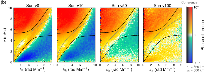
When we look at a slightly higher pair of heights, $z=560$ km and $z=600$ km as shown in Figure 1(b), we notice that there are differences in the phase spectra between the models, unlike what we see in the case of the lower pair of heights (compare with Figure 1(a)). The non-magnetic model and the weak field model still show upward propagating (negative phase difference) IGWs, whereas the models with stronger magnetic fields show downward propagating IGWs as is evident from the positive phase difference (reddish region) in the IGW region of the phase spectra. In summary, despite showing similar phase spectra in the lower atmosphere, irrespective of the average flux density, we see that the phase spectra is modified by the fields in the higher layers, and shows downward propagating waves in the stronger field case.

4.2 Mechanical flux spectra

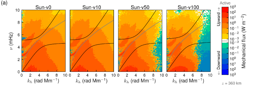
To understand the energy transport by waves, we will now turn our attention to the energy flux spectra represented on the $k_{h}-\omega$ dispersion relation diagram. The time-averaged active component of the mechanical flux is given by the perturbed pressure-velocity ( $\Delta p$ - $v$ ) co-spectrum (see Equation (4) of Paper I). In Figure 2, we show the vertical flux of the active mechanical energy density for the four models at two representative heights. We have chosen $z=360$ km and $z=700$ km, in order to reveal the effects of the strongly varying average plasma- $\beta$ (the ratio of gas pressure to magnetic pressure) with the magnetic flux density at the upper of the two heights. The leftmost plot in both figures each show the energy flux spectrum for the non-magnetic model (Sun-v0), the remaining plots are for the magnetic models Sun-v10, Sun-v50, and Sun-v100, from left to right. Examining the region below the lower propagation boundary of the $k_{h}-\omega$ diagram in the lower atmosphere ( $z=360$ km, Figure 2(a)), we see that all the fluxes are positive (yellow-red colorscale). This clearly shows that the energy transport is predominantly in the upward direction in the order of 1-10 Wm^-2 in the given frequency-wavelength range. Comparing this to Figure 1(a), we clearly see here the signature of IGWs with their vertical component of the phases being opposite to the propagation direction. This is in contrast with the acoustic waves, occupying the region above the upper propagation boundary, which show the same direction for the phase and energy transport.

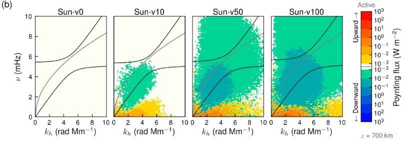
However, as we go higher up in the atmosphere, at $z=700$ km (shown in Figure 2(b)), we notice that for stronger fields, the energy flux is downwardly directed (green region) in regions where the excited IGWs (see Figure 1(a)) are located. The height of 700 km corresponds to a low plasma- $\beta$ region for the case of strong magnetic fields (for $B_{z}$ typically greater than 50 G) and high- $\beta$ region for the case of weak magnetic fields, which is an important difference that will be examined later in Section 5.1. This shows us that as the fields get stronger, there is more downward propagating IGWs in the upper atmosphere transporting their energy downwards. We would like to caution the reader, that for this height and the stronger field cases, the propagation boundary in Figure 2(b) is just shown to guide the eye but otherwise has lost its physical meaning. Instead, one would have to consider the complete MAG dispersion relation, which is different from the acoustic-gravity dispersion relation. The lower part of the $k_{h}-\omega$ dispersion relation diagram correspond to the slow-MAG branch, where the flux remains upward directed and it gets stronger with increasing field strength (the red regions below $\nu=1$ mHz).

4.3 Poynting flux spectra

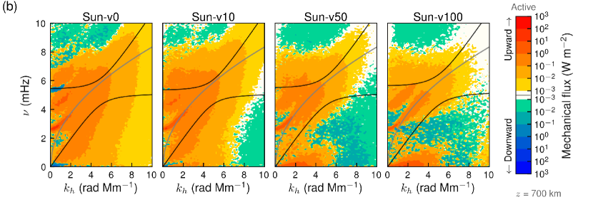
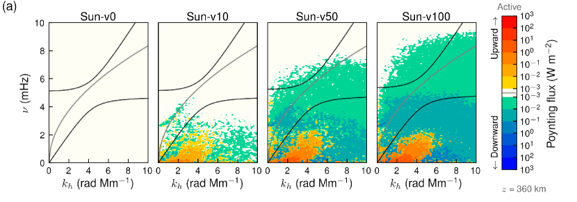
We will now look at the active component of the Poynting flux that can reveal more information about propagating Alfvén waves in the domain. The time-averaged flux of electromagnetic energy is given by the real part of the complex Poynting vector (see for e.g. 1982MINTF...8.....L; 1998clel.book.....J). In our case, this can be readily obtained by taking the co-spectrum of the vector product of perturbed field, $\bm{B^{\prime}}$ , and $\bm{v\times B_{0}}$ . In Figure 3, we show the spectra of the vertical component of the Poynting flux from the magnetic models at two different heights, $z=360$ km and $z=700$ km, respectively. Although, the fluxes are a few orders of magnitude smaller than the mechanical flux presented in Figure 2, it is interesting to look at how they behave as the magnetic fields become stronger and what this may tell us about propagating Alfvén waves.

Looking at Figure 3(a), we see that for the lower layer, which is located in the high- $\beta$ regime for all models, the Poynting flux in the IGW/gravito-Alfvén regime (below the lower propagation boundary) shows a positive sign, meaning upwardly directed. Compare this to the phase difference and the mechanical flux transport, both of which show that the energy is predominantly transported in the upward direction.

But as we go higher up in the atmosphere (see Figure 3(b)), we notice that these fluxes are negative in the regions where the IGWs are excited by the convection, which means that the Poynting flux, similar to the mechanical flux, is downwardly directed. This effect gets stronger the stronger the field (compare Sun-v50 and Sun-v100). This clearly shows us that there are barely any upward directed Alfvén waves. Here again, we remind that not the complete MAG dispersion relation is considered.

5 Discussion

We saw that the phase spectra of the IGWs at the lower height remain the same irrespective of the average magnetic flux density of the model atmosphere. However, there are differences in the phase spectra as well as in both the mechanical and Poynting flux as we go higher up in the atmosphere. In order to explain this behavior with height we will explore some of the properties of the atmosphere in terms of the wave generation and propagation in the presence of magnetic field. Furthermore, we will also discuss about what this means for the energy transport by waves.

5.1 Atmospheric properties

We will first look at the physical structure and dynamics of the magnetoconvection occurring in the different models that we have computed. As noted in the Section 2, the model atmospheres differ in the initial magnetic flux density that was added to an otherwise non-magnetic medium. We build all the models from the same thermally relaxed initial state, as a result of which the different models show very similar thermal properties. Significant differences are evident only when comparing the properties of the atmosphere where magnetic effects dominate. The effect of magnetic field is seen in the propagation properties of the waves only in the higher layers, while the generation of the waves in the near-surface region remain the same across the different models as evident from the phase and energy flux spectra presented in the previous section.

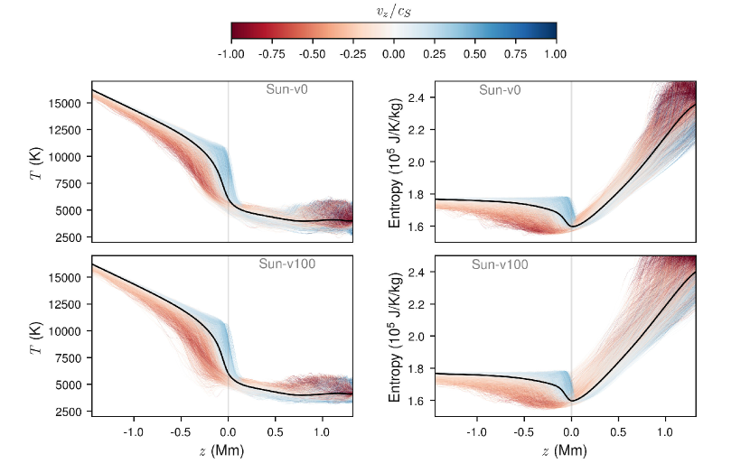
Let us first look at the thermal profile of the models that we study here. Figure 4 shows the mean temperature (left panels) and specific entropy (right panels) as a function of height (black curve) for a single snapshot taken 4 hours after the start of the simulation for the non-magnetic (top panels) and a magnetic model with the largest average magnetic flux density (bottom panels). In the background we show the excursion of the corresponding temperature and specific entropy observed at the same time instance over the whole domain. The curves are color-coded to show the vertical velocity (normalized by the local sound speed) in the voxels along the $z$ -direction, where blue means an upward velocity and red means downward velocity. For clarity, the position of $z=0$ km height level is shown with a gray vertical line to mark the separation of convective and the radiative regions.

Just below the optical surface, i.e. below $z=0$ km, the ascension of hot buoyant convective parcels are clearly visible as blue shade above the mean temperature profile. Regions with lower temperatures than the mean, appearing red, are the cool denser parcels flowing down in the intergranular lanes. Above the surface, from $z=0$ to about 100 km, we see that the hot voxels have overshot slightly into the stable layers, beyond which they radiatively cool down and are dominated by downward parcels as evident from the red shade. This overshooting hot material, that we see in all the models, are thought to result in the excitation of the IGWs. Further up, we see a mixture of upward and downward flowing plasma.

The sudden drop in temperature near the surface due to the switch from a convective interior to a radiative atmosphere is clearly evident in all the models. In the right panels of Figure 4, we can see that the entropy rich (above the mean value) upwellings of the convective parcels in blue shade below the $z=0$ km level. Once these parcels enter the stably stratified radiation zone, they radiate away their heat and thereby loose entropy and fall back. This can be seen in the entropy-deficient parcels moving downward (red shade) in the convection zone. Just above the surface, the down falling matter is entropy rich as a result of heating from below. In the magnetic models, however, there is additional, presumably magnetic heating that results in slightly higher entropy of the down falling material relative to the non-magnetic model. The steady increase in entropy as a function of height in the atmosphere is visible in all models as a consequence of radiative absorption. It is clear from Figure 4 that the launching regions of IGWs are the near-surface overshooting, which generates predominantly upward propagating waves above this layer. However, these regions are the places where we also see kG fields accumulated in intergranular lanes. The question is how do they influence the wave generation.

5.2 Wave generation and propagation

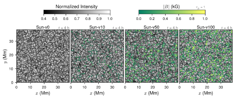
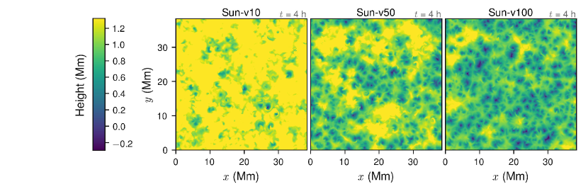
Figure 5 shows the emergent bolometric intensity from the four models taken 4 hours after the start of the simulation. Also shown is the absolute magnetic flux density in color scale for the magnetic models. The accompanying animation shows the time evolution of the granular pattern and the magnetic map over the entire duration of the simulation. One notices that the weakest magnetic model, Sun-v10, has very few concentrations of kG fluxes mostly in the vertices where several granules meet, where most of the fluxes accumulate due to strong convergent flows. Models with stronger initial field strengths have fluxes in the entire periphery of individual granules as well. Comparing this with the phase spectra of the IGWs, which do not differ much among models, clearly shows that the kG fields that are present in the intergranular lanes do not have any influence on the generation of IGWs.

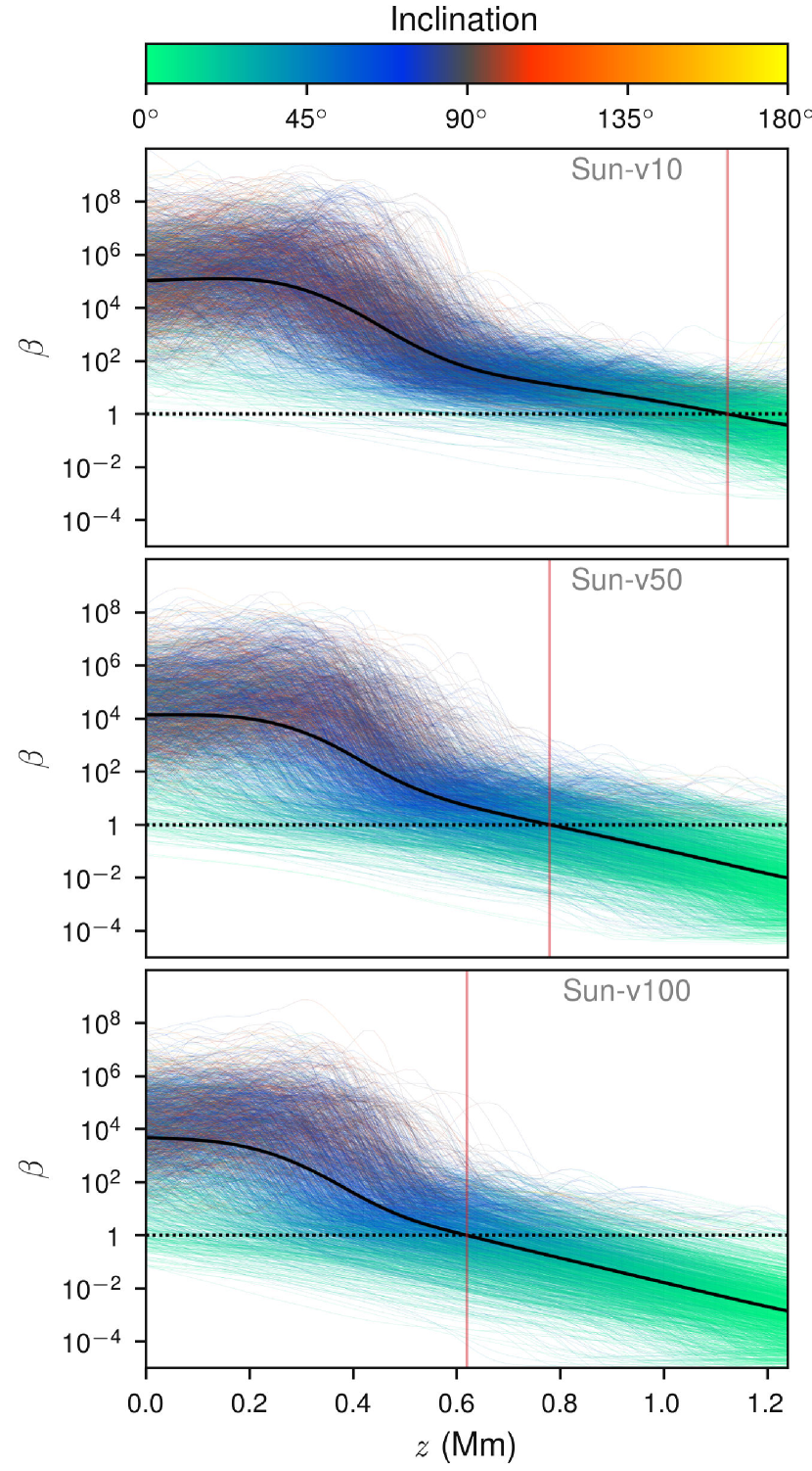
However, this is not the case for the upper layers where we do see an influence of the magnetic fields on the phase spectra and the energy flux spectra. The most important property of a magnetic atmosphere relevant to the study of waves is the plasma- $\beta$ . For magneto-atmospheric waves, it is well known that the $\beta$ =1 surface is a crucial layer across which mode coupling can occur. At locations of strong magnetic field the $\beta$ surface dips, so that waves propagate differently within small-scale flux-concentrations compared to the propagation in nearly field-free quiet regions. For IGWs, changes on these small length scales do not have a major effect, rather it is the average properties that matter. Since we consider different magnetic field strengths, a clear distinction occurs in the average plasma- $\beta$ of these models. Figure 6 shows the height of the plasma- $\beta$ =1 layer from the same snapshot for each models. This shows us the height above which the IGWs are likely to be strongly affected and how the height varies with varying average magnetic flux density.

Figure 7 shows the plasma- $\beta$ profiles as a function of height in the three models taken from the same snapshot as used in Figures 4. The average value as a function of height is marked by the black curve and the $\beta$ =1 value is marked by the dotted line to aide the reader. The background curves show the profiles in all the domain and are color-coded to represent the inclination of the field with respect to the vertical direction. For the weak magnetic field case, Sun-v10, the gas pressure dominates magnetic pressure nearly everywhere in the atmosphere except in the very top part, resulting in a significant portion of the atmosphere to be a high- $\beta$ atmosphere. But as the magnetic fields get stronger, an extended part of the atmosphere in the top layers becomes low- $\beta$ . The average plasma- $\beta$ profile moves down in the atmosphere. This is evident from Figure 7, where we see that the average level of $\beta=1$ is at $z=800$ km for the Sun-v50 case and at $z=600$ km for the Sun-v100 case, compared to $z=1100$ km for the Sun-v10 case. These heights are indicated as red vertical lines to aide the reader. A consequence of this is that the IGWs in the low field strength case can propagate unhindered as far out as 1000 km, whereas for the stronger field strength case, the height limit is around 700 km. It is clear from Figure 7 that above the $\beta=1$ layer the fields are mainly vertical (green shade), so that with increasing field strength, models show an extended region of predominantly vertical magnetic fields, which is a consequence of the top boundary condition.

The propagation properties of IGWs can be clearly understood in terms of the phase spectra presented in Section 4.1. Despite the presence of kG fields in the surface layers, the similar nature of the phases in the IGW regime between non-magnetic and all magnetic field models, confirms that the granular updrafts are the main source region of these waves, as the differences between the models concerns the intergranular lanes only. However, the higher layers show a completely different behavior in the phase spectra, which is a result of the differences in the average plasma- $\beta$ with height of the three magnetic models.

5.3 Energy Transport

Let us now turn to the main objective of this paper. We are interested in estimating the energy transported by wave-like motions, particularly internal wave fluctuations, and in getting an insight on how magnetic fields may influence this transport. The primary reason why waves are considered important is because they are a carrier of mechanical energy and momentum between the deep photosphere and the upper solar atmosphere without the need of any material transport. Knowing the upward flux of mechanical energy associated with the waves as a function of height can tell us at which layer the energy gets utilized. As we are looking at magneto-atmospheric waves, we also need to consider the electromagnetic work done by the waves which is given by the associated Poynting flux. The Poynting flux is then likely converted into thermal and bulk kinetic energy by magnetic dissipation and by the action of the Lorentz force (2004ASPC..312..357S). In the following, we will discuss how wave energy fluxes are estimated from real observations and compare them to the fluxes calculated using a different approach from our simulations.

The flux estimates for various observed wave phenomena rely on the fact that the energy flux can be determined directly from the mean energy density and the group velocity of the wave under consideration. Although this is generally true for any type of waves, it is often the quantities that go into this simple expression that are prone to uncertainties. Firstly, a reliable estimate of the mean energy density depends on how closely the model atmosphere, from where the mass densities are determined, matches the observed region. Secondly, the group velocity of a simple observed wave is often difficult to estimate, let alone for a dispersive wave for which the concept of group velocity breaks down. In most cases, it is not explicitly stated as to where the group velocity estimates come from (2012SoPh..279...43W).

For the acoustic waves, the group velocity can be obtained using the dispersion relation. The vertical component of the group velocity is given as (2006ApJ...646..579F; 2009A&A...508..941B),

v_{g,z}=\partialderivative{\omega}{k_{z}}=c_{s}\sqrt{1-(\omega_{ac}/\omega)^{2}}

(1)

which asymptotes to the local sound speed ( $c_{s}$ ) for large frequencies, while becoming zero for lower frequencies as one approaches the acoustic cut-off ( $\omega_{ac}$ ). Assuming a speed of sound and the acoustic cut-off frequency from a model atmosphere, one can estimate the energy flux in the desired frequency bin. 2009A&A...508..941B showed that at a height of 250 km the low frequency range (5-10 mHz) contributes more to the cumulative acoustic flux of 3000 W m^-2 than the flux in the high-frequency (10-20 mHz) range. However, 2005Natur.435..919F; 2006ApJ...646..579F report that the fluxes in the acoustic range is insufficient by a factor of 10 to balance the radiative losses.

For the IGWs, it is quite tricky as these waves do not propagate purely vertically. The vertical component of the group velocity ( $v_{g,z}$ ) is given in the incompressible limit as (1981ApJ...245..286P; 2016A&A...588A.122P),

v_{g,z}=\partialderivative{\omega}{k_{z}}=\left(\frac{\omega}{N}\right)^{2}\frac{\sqrt{N^{2}-\omega^{2}}}{k_{h}},

(2)

which can be written in terms of the vertical phase velocity ( $v_{ph,z}$ ) as (2011A&A...532A.111K),

v_{g,z}=-v_{ph,z}\sin^{2}({\omega/N}).

(3)

Thus, to estimate the energy flux, the main ingredient is the vertical component of the phase velocity. 2008ApJ...681L.125S determine the energy flux of the IGWs using the $v-v$ phase spectra from Interferometric BIdimensional Spectrometer (IBIS; 2006SoPh..236..415C) observations. The $v-v$ phase difference spectra are first converted to phase travel time spectra and then to phase velocity spectra under the assumption that the difference between the two line formation heights is known. The group velocity spectra are then determined from the phase velocity according to Equation (3). The energy flux spectra are finally obtained by using the plasma density from the VAL model C (1976ApJS...30....1V) and the mean squared velocity from Doppler shifts. 2008ApJ...681L.125S found the energy flux in the IGW region to be 20800 W m^-2 at a height of 250 km dropping to 5000 W m^-2 at a height of 500 km in the atmosphere. 2011A&A...532A.111K find a lower flux of 4100-8200 W m^-2 at 380 km and 700-1400 W m^-2 at 570 km. The main reason for this discrepancy is thought to stem from the fact that 2008ApJ...681L.125S overestimate the vertical group velocity because they do not consider the atmospheric transmission (2011A&A...532A.111K).

With the help of numerical simulations, we can get an estimate of the energy fluxes without needing the group velocity, since we have access to all the physical quantities everywhere in the model atmosphere. We can assume that the fluctuations caused by waves are weak and that there are no strong background flows present. In such a scenario, the non-linear MHD equations can be linearized by expanding quantities in terms of a static background and perturbations and neglecting terms greater than first order powers of the perturbed quantities. By algebraic manipulation and casting the equations for perturbations in the form of a conservation law, one can derive an energy density and a flux of energy density associated with linear wave motion. Even for a weak fluctuation this assumption is not valid for a long timespan as non-linearities eventually arise due to the sole property of the governing equations. Also, the wave energy density is conserved only for the case of a uniform stratification (1968RSPSA.302..529B), i.e for an atmosphere with constant Brunt-Väisälä frequency ( $N$ ). In the models that we study here the $N$ varies with height. Therefore, we would like to caution the reader that the definition of linear wave energy density and flux does not represent the total energy density and flux associated with a wave. To get a better estimate of the energy density and flux, we would have to include the second order terms (1985GApFD..32..123L; 2017ApJ...837...94T). Having a time dependent background and spatial inhomogeneity, it is evident that the total wave energy is not conserved. The wave can continuously exchange energy with the background, raising concern on casting the wave energy equation in the form of a conservation law. Despite all these concerns, one can say that the linear energy flux considered here gives the leading order contribution to the conserved pseudoenergy flux (1978JFM....89..647A; 1984AnRFM..16...11G).

The “linear” wave energy flux in a MHD system is made up of mechanical energy flux and the Poynting flux,

F_{\rm{wave}}=\displaystyle p^{\prime}\bm{v}+\frac{1}{4\pi}\quantity[\bm{B^{\prime}\times(v\times B_{0})}],

(4)

where, $p^{\prime}$ is the pressure perturbation, $\bm{v}$ is the velocity, $\bm{B_{0}}$ is the equilibrium magnetic field and $\bm{B^{\prime}}$ is the field perturbation. The first term on the right hand side of Equation (4) represents the rate of mechanical work done per unit area by a volume on a adjacent volume due to the excess pressure as a wave propagates across the volume interface. Often quoted as the acoustic flux, in this context, we would rather call it the mechanical flux, since it represents the total mechanical work done by all waves, as most waves in the medium cause pressure fluctuations as they propagate. This is different from the way in which the mechanical fluxes are estimated from observations. The second term in Equation (4), represents the Poynting flux, the flux of electromagnetic energy, which is also carried by all the waves in the magneto-acoustic-gravity coupled system that we consider. There is mechanical and Poynting flux associated with all the waves in the medium and therefore, in the time domain, it is not possible to distinguish between these fluxes and map them to a specific wave motion. However, it is worthwhile to estimate the contribution to the total mechanical and the total Poynting flux that arise exclusively from wave-like motions in the domain.

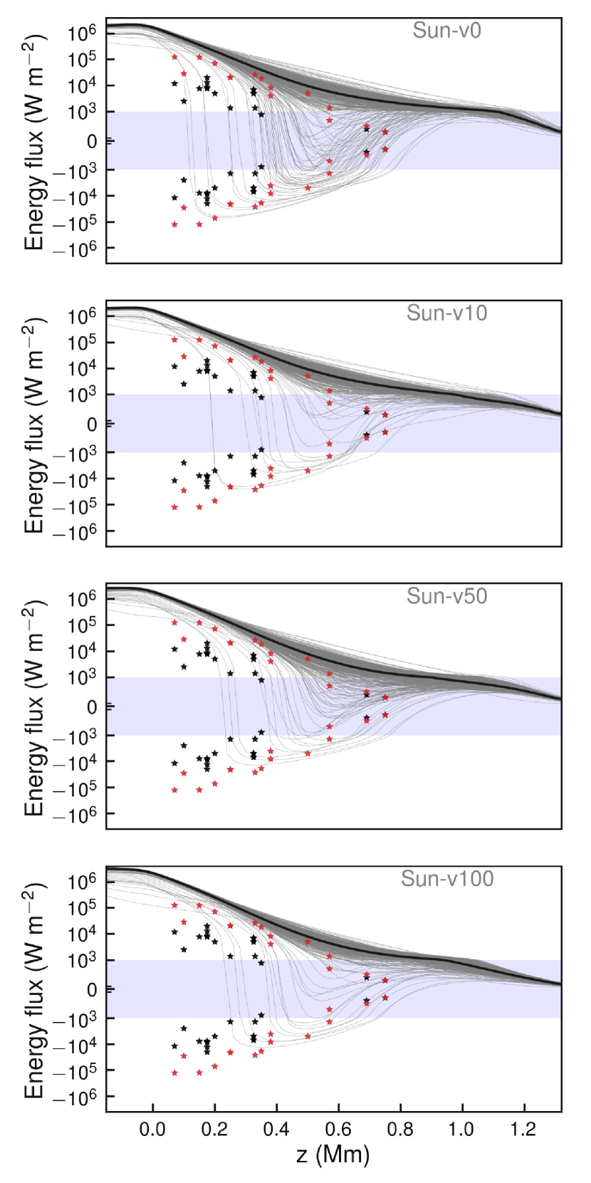
We first look at the vertical mechanical energy flux density ( $F_{M}$ ) as expressed by the first term in the rhs of Equation (4). Figure 8 shows the horizontally averaged mean $F_{M}$ (black curve) as a function of height calculated from the four models. In the background we show the excursion of mean $F_{M}$ for individual snapshots over the duration of the simulation. It is clear from the height dependence of mechanical energy flux that we do not see much difference between the non-magnetic and the magnetic cases. However, we notice that there is a small scatter of locations with the mean flux directed downward (negative energy flux) in the middle part of the atmosphere around $z=0.6$ Mm. It is not obvious whether this scatter can be related to waves that are present in the box. The energy flux obtained from observations (2011A&A...532A.111K; 2008ApJ...681L.125S; 2010ApJ...723L.134B) are marked as asterisks on all the plots. This includes the energy flux for the acoustic (marked in black) as well as the IGWs (red). As can be seen, close to the surface the fluxes obtained from observations ( $\sim 10^{4}$ – $10^{5}$ Wm^-2) are close to an order of magnitude less than what we see in the simulations ( $10^{6}$ Wm^-2). However, this difference is less pronounced as we go higher up in the atmosphere. Here, we also show the observed fluxes with the negative sign as a reference for comparing the negative (downward) fluxes that we obtain in simulations.

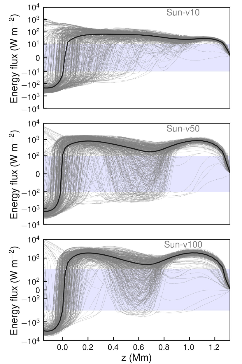
The horizontally averaged vertically directed Poynting flux ( $F_{P}$ ; black curve), as defined by the second term in the rhs of Equation (4), as a function of height is shown in Figure 9. In the background we show the excursion of mean $F_{P}$ for individual snapshots over the duration of the simulation for all the three magnetic models. In all the magnetic models, the Poynting flux close to the surface at $z=0$ km and below is directed downward as a result of the strong downdrafts in the intergranular lanes that carry with them magnetic flux, whereas, close to the surface and above, the overshooting material carries magnetic flux upwards resulting in a net upward Poynting flux (2008ApJ...680L..85S). This can be clearly seen for all three models in Fig. 9. However, we notice that there is a large scatter of fluxes with downward contribution. This scatter seems to depend on the magnetic field strength and consequently on the location of the mean plasma- $\beta$ =1 layer. Models with a strong field show a downward directed Poytning flux close to the layer of plasma- $\beta$ =1, extending over a broad height range below this layer. Models with weak fields, show considerably less downward directed Poynting flux. It is clear that a major contributer to the downward Poynting flux come from the region of IGWs as evident from the energy flux spectra presented in Section 4.3.

5.4 Limitations of the current study and future outlook

In this section, we will briefly mention some of the limitations of the current study and future direction. One of the major drawback of the present work is that the results obtained here are based on spectral analysis done on geometrical heights. This makes it hard to compare with observational data as they are mainly obtained from spectral maps that probe constant optical depths. A further exploration of this will require, performing the cross-spectral analysis on velocity data obtained from constant optical depths, or doing a spectral synthesis of different lines and performing the cross-spectral analysis on the estimated Dopplergrams, which will be explored further in a forthcoming paper.

The current simulation set-up with a rather coarse grid resolution of 80 km is sufficient to capture the emergent IGW spectra. Increasing the resolution may have an effect on the overall spectra of IGWs, as the granulation pattern is seen to be more structured in higher resolution simulation. However, due to the computationally expensive nature of such simulation, a study on the effect of grid resolution on the emergent IGW spectra was not pursued in this paper. In terms of boundary conditions, we have not studied the effect of how changing the lateral and top boundary condition will affect the propagation of waves. For the lateral boundary, we are restricted to use a periodic boundary condition as the fast Fourier transform algorithm assumes that the boundaries are periodic. However, imposing a periodic side boundary condition restricts the maximum wavelength of the waves to the length of the box. The top boundary condition forces the field to be vertical, thereby restricting us to study a magnetic environment that has only predominantly vertical magnetic fields. This however, is the case for all the models and thus makes it easy to do a comparative study. Further analysis with predominantly horizontal fields may reveal whether a coupling to low- $\beta$ gravito-Alfvén waves is possible. In this case the angle of attack of these obliquely propagating waves will be mainly parallel to the fields and therefore have a chance to propagate into the upper layers.

We would like to mention here the effect of the Alfvén speed limiter that has been used in this study. Firstly, this speed limiter may affect waves with horizontal phase velocity greater than 40 km s^-1 which fall mainly in the high-frequency part of the $k_{h}-\omega$ diagram, which does not include the IGW region. Secondly, waves with vertical phase velocity larger than 40 km s^-1 fall close to the propagation boundary according to Eq. 1 in Paper I and are insignificant. Therefore, we expect that the major part of the IGW spectrum is unaffected by the use of the Alfvén speed limiter.

Finally, we would like to caution the reader that the diagnostic diagram for the complete spectra of MAG waves in a uniform magnetic field medium is drastically different from that of the acoustic-gravity waves (considered here and in Paper I). The fact that we have three distinct branches of coupled waves, viz. the fast MAG, the gravito-Alfvénic, and the slow-MAG, and that their behavior in the diagnostic diagram vary depending on the magnetic field inclination relative to the wave vector and depending on the plasma- $\beta$ , brings more variety and complexity to the diagnostic diagram (for a detailed reference see 2004prma.book.....G, Chapter 7, Section 7.3.3). In the low photosphere we still have a predominantly high- $\beta$ atmosphere, which makes it easier to use the diagnostic diagram for acoustic-gravity waves. As we move higher in the atmosphere, we approach the surface $\beta$ =1 and move into the low- $\beta$ regime, where the slow- and fast-MAG branch becomes more relevant and the three different branches look very different for different orientation of the magnetic field relative to the propagation vector. These effects are not taken care of in the present study since we focus mainly on regions with high- $\beta$ where the dispersion relation approximates that of the acoustic-gravity waves.

More recent work by 2017ApJ...842...37B have quoted a value of 35 G as the average magnetic flux density of the quiet Sun region. Comparing it with the cases that we study in this paper, this would coincide with a model intermediate to Sun-v10 and Sun-v50, for which the average height of plasma- $\beta$ =1 layer would correspond to around $z=900$ km. Therefore, we argue that IGWs in the quiet Sun should be easily detectable up to a height of 900 km. Quasi-simultaneous measurements of 2D velocity fields at multiple heights, obtained from photospheric lines, with a reasonably large field-of-view (40 x 40 Mm²) and an observational duration of 3 hours will provide a good spectral resolution in the $k_{h}-\omega$ to identify the waves. Continuous observation with a cadence of less than 60 seconds ( $\nu_{\rm max}=8.33$ mHz) and with a moderate spatial resolution of up to 300 km ( $k_{h,{\rm max}}=10$ rad Mm^-1) can sufficiently capture the spectral region of the emergent IGWs. We predict that the observed spectra of the IGWs obtained from same spectral lines will likely show differences among internetwork and the more magnetically dominated plage regions. Future observations using DKIST could help elucidate and validate our models.

6 Conclusions

Our investigation of the gravity-wave phenomena in the solar atmosphere has shown us that these waves are naturally excited by the overshooting convection. We study here the effect of magnetic field strength on the generation and propagation properties of IGWs in four different models of the solar atmosphere. This allows for a direct comparison of wave generation between magneto-atmospheres representative of different regions of the solar surface, like internetwork, network, and plage regions. We find that in the near surface photospheric layers the emergent IGW spectra are unaffected by the presence as well as by the strength of the magnetic field. IGWs are generated with considerable amount of wave flux independent of the average value of the magnetic flux density in the wave originating region in the quiet Sun and they propagate into higher layers. With increasing initial field strength, the magnetic flux tends to accumulate at the periphery of the granules. The main excitation region of IGWs are these granular upwellings into the stable region above.

We find that the energy fluxes obtained from observations are close to an order of magnitude less than what we see in the simulations in the lower part of the atmosphere. In terms of wave energy fluxes, three conclusions can be drawn from the present study. Firstly, the energy fluxes in the IGWs region are larger by an order of magnitude than the fluxes in the acoustic waves in the lower part of the atmosphere where plasma $\beta$ is high. Secondly, the mechanical flux dominates the total wave energy fluxes and is several orders of magnitude larger than the Poynting flux below the plasma- $\beta$ =1 level. Thirdly, the height dependent horizontally averaged vertically directed Poynting flux shows large scatter with a downward component below locations where the average plasma- $\beta$ =1. A closer look at the Poynting flux in the frequency domain reveals that there is no upward component for models of strong field in the IGW regime and hence no mode-coupling of IGWs to Alfvén waves across the $\beta$ =1 surface, as a consequence of the predominantly vertical fields. In the case of mechanical energy transport up to the heights where the plasma $\beta$ remains greater than 1, the IGWs are quite dominant and surpass the acoustic energy flux. But depending on the magnetic field strength the energy in the IGWs can be redirected and restricted to the near surface regions never reaching higher layers. This suggests that IGWs may not be abundant above the plasma- $\beta$ =1 surface and therefore are likely to be undetectable in observations of chromospheric layers and therefore they may not directly or indirectly contribute to the heating of layers above plasma- $\beta$ less than 1. In the upper photosphere, however, their propagation properties depend on the average magnetic field strength and therefore these waves can be used as a diagnostic for the average magnetic field properties of these layers.

This work was supported by the German Deutsche Forschungsgemeinschaft, DFG grant RO 3010/3-1. We thank the anonymous referee for his/her detailed comments and suggestions which significantly improved the presentation of the paper. G.V. acknowledges the helpful discussions with Nazaret Bello González and the CO⁵BOLD community. The authors are grateful to the developers of NumPy, SciPy, Matplotlib, Cython, and Astropy python projects for providing the tools for carrying out this work. This research has made use of NASA’s Astrophysics Data System.

Internal Gravity Waves in the Magnetized Solar Atmosphere. II. Energy Transport