Hydrodynamic Interaction between Two Elastic Microswimmers
Abstract
We investigate the hydrodynamic interaction between two elastic swimmers composed of three spheres and two harmonic springs. In this model, the natural length of each spring is assumed to undergo a prescribed cyclic change, representing the internal states of the swimmer [K. Yasuda et al., J. Phys. Soc. Jpn. 86, 093801 (2017)]. We obtain the average velocities of two identical elastic swimmers as a function of the distance between them for both structurally asymmetric and symmetric swimmers. We show that the mean velocity of the two swimmers is always smaller than that of a single elastic swimmer. The swimming state of two elastic swimmers can be either bound or unbound depending on the relative phase difference between them.
I Introduction
Microswimmers are small machines that swim in a fluid and they are expected to be used in microfluidics and microsystems Lauga09 . Over the length scale of microswimmers, the fluid forces acting on them are dominated by the frictional viscous forces. By transforming chemical energy into mechanical energy, however, microswimmers change their shape and move efficiently in viscous environments. According to Purcell’s scallop theorem, time-reversible body motion cannot be used for locomotion in a Newtonian fluid Purcell77 ; Lauga11 . As one of the simplest models exhibiting broken time-reversal symmetry, Najafi and Golestanian proposed a three-sphere swimmer (NG swimmer) Golestanian04 ; Golestanian08 , in which three in-line spheres are linked by two arms of varying length. Recently, such a swimmer has been experimentally realized by using colloidal beads manipulated by optical tweezers Leoni09 , ferromagnetic particles at an air-water interface Grosjean16 ; Grosjean18 , or neutrally buoyant spheres in a viscous fluid Box17 .
Using the NG swimmer model, Pooley et al. showed that the interaction between two swimmers depends on their relative displacement, orientation, and phase, leading to motion that can be either attractive, repulsive, or oscillatory Pooley07 . Scattering of two NG swimmers was also investigated on the basis of the time-reversal invariance of the Stokes equation Alexander08 . Later Farzin et al. reexamined the hydrodynamic interaction between two NG swimmers and concluded that the long-time swimming states are different between moving in the same and opposite directions Farzin12 . To understand hydrodynamic coupling for stochastic swimmers, on the other hand, Najafi and Golestanian studied the correlated motion of a three-sphere swimmer and a two-sphere system Najafi10 . They calculated the swimming velocities as functions of the statistical transition rates for the conformational changes.
Recently, the present authors have proposed a generalized three-sphere microswimmer model in which the spheres are connected by two harmonic springs, i.e., an elastic microswimmer Yasuda17 . Compared with the NG swimmer, the main difference of the elastic swimmer is that the natural length of each spring (rather than the arm length) oscillates in time and is assumed to undergo a prescribed cyclic change. As a result, the sphere motion in our model is determined by the natural spring lengths, representing the internal states of a swimmer, and also by the force exerted by the fluid. We have analytically obtained the average swimming velocity as a function of the frequency of the cyclic change in the natural length Yasuda17 . In the low-frequency region, the swimming velocity increases with frequency and it reduces to that of the NG swimmer Golestanian04 ; Golestanian08 . Conversely, in the high-frequency region, the velocity decreases with increasing frequency. We note that similar models were proposed by other people Dunkel09 ; Pande15 ; Pande17 , while our elastic swimmer model was further extended to thermally driven elastic micromachines Hosaka17 .
In this work, we investigate the hydrodynamic interaction between two elastic three-sphere swimmers that are confined in one-dimensional space and moving in the same direction. We first derive a general expression for the average velocities (over a period of one cycle) of two hydrodynamically interacting three-sphere swimmers as a function of the distance between them. Using this general expression, we then calculate the explicit forms of the average velocities of two identical elastic microswimmers. We show that the mean of the two average velocities is always smaller than that of a single elastic swimmer, whereas the velocity difference depends on the relative phase difference in the natural lengths between the two swimmers. As a result, the swimming state of two elastic swimmers can be either bound or unbound depending on the relative phase difference.
In Sect. II, we first discuss the motion of two interacting three-sphere microswimmers. In Sect. III, we calculate the average velocities of two interacting elastic swimmers, and further discuss the mean and the difference between the two average velocities. The average velocities of two symmetric elastic swimmers is discussed in Sect. IV. In Sect. V, we discuss the interaction of two NG swimmers by considering the low-frequency limit of our results. Finally, a summary of our work and some discussion are given in Sect. VI.
II Two interacting three-sphere swimmers
As shown in Fig. 1, we consider two general three-sphere swimmers in a viscous fluid characterized by shear viscosity . Each swimmer consists of three hard spheres of the same radius connected either by two arms (NG swimmer) or by two harmonic springs (elastic swimmer explained in the next section) A and B. The positions of the three spheres in the left (L) swimmer are denoted by , , and in a one-dimensional coordinate system, while those in the right (R) swimmer are denoted by , , and . We also assume without loss of generality. The distance between the two swimmers is defined by the positions of the middle spheres, i.e., .
Owing to the hydrodynamic interaction, each sphere exerts a force on the viscous fluid and is subjected to an opposite force from it. Denoting the velocity of each sphere by and the force acting on each sphere by (), we can write the equations of motion of each sphere as
| (1) |
where the details of the hydrodynamic interactions are taken into account through the mobility coefficients . Within Oseen’s approximation, which is justified when the spheres are considerably far from each other (), the expressions for the mobility coefficients can be written as
| (2) |
We remark here that although the two swimmers are aligned along the one-dimensional axis, the spheres are interacting through the three-dimensional hydrodynamic interaction. Furthermore, we require two force-free conditions of the two swimmers, i.e.,
| (3) |
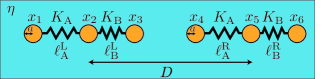
Let us denote the average arm length (NG swimmer) or the average natural length (elastic swimmer) by , and also introduce the four displacements of the springs with respect to for the left and right swimmers as
| (4) | |||
| (5) |
Then the four kinematic constraints are given by taking the time derivative of the above relations:
| (6) | |||
| (7) |
We note here that Eq. (1) implies six coupled equations. Together with the two force-free conditions in Eq. (3) and the four kinematic constraints in Eqs. (6) and (7), we have sufficient equations to solve the twelve unknowns, namely, and (). Finally the average velocities of the left and right swimmers can be obtained by
| (8) |
where averaging is performed by time integration in a full cycle.
Under the condition that the two swimmers are far from each other and the deformations are small compared with the average arm length , i.e., , one can perform a perturbative calculation to obtain the average velocities as
| (9) | |||
| (10) |
Note that we have kept only up to second-order terms in as in Ref. Najafi10 , meaning that we are also assuming the condition . The first terms on the right-hand side of the above equations represent the average swimming velocity of a single three-sphere swimmer, as previously obtained by Golestanian and Ajdari Golestanian08 . These terms indicate that the average velocity of an isolated three-sphere swimmer is determined by the area enclosed by the orbit of the periodic motion in the configuration space.
The second terms on the right-hand side of Eqs. (9) and (10) are due to the hydrodynamic interaction between the two swimmers. These correction terms decay as with increasing distance because they result from force quadrupoles rather than force dipoles Golestanian08 . In fact, such a cubic dependence originates from the symmetry such that the motion of three-sphere swimmers is invariant under a combined time-reversal and parity transformation Pooley07 . The correction terms in and in are both passive terms because they correspond to the swimming of only the second swimmer. The other correction terms are due to the simultaneous motion of the two swimmers and hence are called active terms Pooley07 ; Farzin12 . We show later that only the active terms depend on the phase difference between the two swimmers.
III Two interacting elastic swimmers
In this section, we consider two interacting elastic three-sphere swimmers, as schematically shown in Fig. 1, and calculate their average velocities. We first assume that these two elastic swimmers have identical structures, whereas the structure of each swimmer can be either asymmetric or symmetric (as separately discussed in Sect. IV). For each swimmer, the two spring constants of harmonic springs A and B are denoted by and , respectively. Then the total energy of these two elastic swimmers is given by
| (11) |
In the above, , , , and are the natural lengths of the respective harmonic springs and generally depend on time. Hence, the six forces in Eq. (1) are given by
| (12) |
For these two elastic swimmers, we assume that the four natural lengths of the springs undergo the following periodic changes in time Farzin12 :
| (13) | ||||
| (14) | ||||
| (15) | ||||
| (16) |
Here, is the common average length as introduced in Eqs. (4) and (5), and are the amplitudes of the oscillatory change, is the common frequency, is the relative phase difference between the two springs within the swimmers, and is the relative phase difference between the left and right swimmers. For each swimmer to move by itself, the time-reversal symmetry of the spring dynamics should be broken, i.e., . In the absence of the hydrodynamic interaction between the two swimmers, they move in the same direction with the same velocity. Although this assumption can be relaxed, the current situation already provides us with very rich dynamical behaviors when they interact hydrodynamically. We also note that the frequency can be different between the two swimmers, but such a study is left as a future work.
It is convenient to introduce a characteristic time scale defined by Yasuda17
| (17) |
Then we use to scale all the relevant lengths and employ to scale the frequency, i.e., . By further defining the ratio between the two spring constants as , the coupled equations can be made dimensionless. These equations can be solved in the frequency domain, and we further obtain in Eqs. (6) and (7) after an inverse Fourier transform Yasuda17 . Since their explicit expressions are somewhat lengthy, we give them in Appendix A. Finally, using Eqs. (9) and (10), we calculate the average velocities and of the two elastic swimmers. Their full expressions are given in Appendix B.

Instead, we show here the mean and the difference between the two average velocities and . The former is given by
| (18) |
where the average velocity of a single elastic swimmer was obtained before as Yasuda17
| (19) |
On the other hand, the velocity difference between the two swimmers is given by
| (20) |
In the above equations, we have introduced four scaling functions defined by
| (21) | ||||
| (22) | ||||
| (23) | ||||
| (24) |
These are the main results of this paper.
Equation (18) indicates that, owing to the hydrodynamic interaction between the two elastic swimmers, the mean velocity is always smaller than irrespective of the relative phase difference . Using the formula in Eq. (18), we point out that the -independent contribution to the correction is due to the passive terms in Eqs. (9) and (10), whereas the -dependent contribution comes from the active terms. The correction to vanishes only when , and the mean velocity is minimized when . In contrast, the velocity difference in Eq. (20) can be either positive or negative depending on the conditions. Obviously, we have when . This is reasonable because the two swimmers should move with the same velocity when the relative phase difference vanishes. A more detailed discussion concerning the velocity difference will be given in the next section for symmetric elastic swimmers.
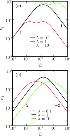
In Fig. 2, we plot the scaling functions and as functions of for , , and Yasuda17 . Note, however, that the cases of and are essentially equivalent because we can always exchange springs A and B, whereas we have defined the relaxation time through as in Eq. (17). As shown in Eq. (19) and previously discussed in Ref. Yasuda17 , the frequency dependence of the average velocity for an isolated elastic swimmer is essentially determined by and . Notice that and for , whereas and for . Hence the average velocity increases for , whereas it decreases for when the frequency is increased Yasuda17 . To ensure the validity of our elastic swimmer model, we assume here that a low-Reynolds-number flow field is justified even in the high-frequency regime .
In Fig. 3, we plot the scaling functions and as functions of for , , and . As shown in Eq. (20), the scaling functions and as well as characterize the frequency dependence of the hydrodynamic interaction between two elastic swimmers. Here, we have and for , whereas and for . When the swimmers are asymmetric such as when and , on the other hand, there are intermediate regions where the scaling functions behave as and . Note that the velocity difference also decreases in the high-frequency regime.
IV Two symmetric elastic swimmers
Having discussed the case of two general (asymmetric) elastic swimmers, we now discuss the case when both elastic swimmers have symmetric structures, i.e., and (or ). In this case, the two average velocities can be simply written as
| (25) | ||||
| (26) |
where the average velocity of a single elastic swimmer now becomes Yasuda17
| (27) |
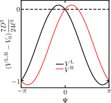
In Eqs. (25) and (26), the -independent terms of correspond to the passive terms as before. In Fig. 4, we plot the -dependences of and when . We see that both and can be larger than for certain ranges of . For , as shown in Fig. 4, we have for and for . However, as we have already explained with Eq. (18) for the general asymmetric case, the mean of and is always smaller than .
Furthermore, the velocity difference is now given by
| (28) |
This is an interesting result because, for and hence , we have for or for . In the former case, the interaction between the two swimmers is repulsive and the distance between them increases as they move, i.e., an unbound state. In the latter case, on the other hand, the interaction is attractive and they form a moving hydrodynamic bound state.
It is worthwhile noting that, in the case of , the average velocity in Eq. (27) behaves as , whereas the velocity difference in Eq. (28) scales as for two symmetric swimmers. Such a difference arises from the presence of the active terms in Eqs. (9) and (10) [or the last -dependent terms in Eqs. (25) and (26)] owing to the simultaneous motion of the two swimmers. According to the above frequency dependences, the velocity difference (for finite ) becomes much smaller than in the limit of , and the two velocities turn out to be identical, as shown later in Eq. (33). A similar argument holds also for because we have and , the latter being the higher-order active contribution.
V Limit of two NG swimmers
The interaction between two asymmetric NG swimmers can be recovered simply by taking the limit of . This is because the spring constants and are infinitely large and the characteristic time scale is infinitely small for NG swimmers. In this limit, the two average velocities defined by become
| (29) |
| (30) |
where the average velocity of a single NG swimmer is Golestanian08
| (31) |
Hence, the mean of and is again given by Eq. (18) in which is replaced by . As mentioned in the previous section, both and are proportional to . The velocity difference, on the other hand, becomes
| (32) |
This result indicates that the velocity difference depends not only on but also on the relative magnitude between and for asymmetric NG swimmers.
For symmetric NG swimmers, i.e., , and are identical and are given by
| (33) |
This result means that the average velocities and of the two symmetric NG swimmers are always smaller than that of an isolated NG swimmer, i.e., . Hence, the possibility of under certain conditions, as shown in Eqs. (25) and (26), is a unique feature of two elastic swimmers. Since for two symmetric NG swimmers, the distance between them remains constant, which is in contrast to the case of two symmetric elastic swimmers [see Eq. (28)]. Such a difference arises from the internal relaxation dynamics of the spheres in elastic swimmers, leading to asymmetric motion of the two springs in each swimmer.
VI Summary and discussion
We have investigated the hydrodynamic interaction between two elastic swimmers consisting of three spheres and two harmonic springs. In this model, the natural length of each spring is assumed to undergo a prescribed cyclic change in time, reflecting the internal states of an elastic swimmer. For two interacting three-sphere microswimmers, we first obtained their average velocities in terms of the distance between them [see Eqs. (9) and (10)]. Using these expressions, we further obtained the explicit forms of the average velocities of two identical elastic swimmers. The mean of the two average velocities was shown to be always smaller than that of a single elastic swimmer [see Eq. (18)]. On the other hand, the velocity difference depends on the relative phase difference between the two elastic swimmers [see Eqs. (20) and (28)]. As a result, the swimming state of two elastic swimmers can be either bound or unbound depending on the relative phase difference.
In this paper, the hydrodynamic interaction was considered only between two three-sphere microswimmers, although there are several other model swimmers. For example, two rigid helices neither attract nor repel each other when they are rotating with zero phase difference Kim04 , two puller-type squirmers undergo a significant change in their orientations after an encounter Ishikawa06 , and two spherical swimmers with spatially confined circular trajectories cause either attractive or repulsive interaction Michelin10 . Using the Quadroar model, Mirzakhanloo et al. showed that two swimmers, which generate flow fields mimicking that of Chlamydomonas reinhardtii, exhibit very rich behaviors Mirzakhanloo18 . The three-sphere swimmer model in one-dimensional space is especially suitable for analytical analysis because it is sufficient to consider only the translational motion, and the tensorial structure of the fluid motion can be neglected.
In our work, we have assumed that the two elastic three-sphere swimmers are confined in one-dimensional space and moving in the same direction. For two NG swimmers, on the other hand, it was shown before that the interaction between them depends on their relative orientation Pooley07 ; Farzin12 . The main reason that we have investigated only the one-dimensional case is that our primary interest is to analytically obtain the frequency dependence of the hydrodynamic interaction between two elastic swimmers, which was not studied before. Another motivation to restrict our study to one-dimensional space is to clarify how the correlation between a three-sphere swimmer and a two-sphere system, as reported in Ref. Najafi10 , can be generalized for two three-sphere swimmers [see Eqs. (9) and (10)]. The future study of the hydrodynamic interaction between two elastic swimmers having different orientations would require a numerical treatment. For instance, the oscillatory motion reported in Refs. Pooley07 and Farzin12 , would be observable only when the space dimension is higher than one.
We have shown analytically that even the interaction between two elastic microswimmers can be complicated, depending on the relative displacement, structure, and phase difference. Nevertheless, it is possible and straightforward to increase the number of interacting swimmers as long as the assumption of low-Reynolds-number hydrodynamics is valid and the swimmers are confined in one-dimensional space. We believe that the present analysis of the hydrodynamic interaction between two swimmers will be useful in studying the collective behavior of a large number of self-propelled microswimmers immersed in a viscous fluid Stenhammar17 ; Filella18 .
Acknowledgements.
We thank S. Al-Izzi, H.-Y. Chen, Y. Hosaka, T. Kato, H. Kitahata, Y. Koyano, and R. Okamoto for fruitful discussions and helpful suggestions. K.Y. acknowledges support by a Grant-in-Aid for JSPS Fellows (Grant No. 18J21231) from the Japan Society for the Promotion of Science (JSPS). S.K. acknowledges support by a Grant-in-Aid for Scientific Research (C) (Grant No. 18K03567) from the JSPS.Appendix A Displacements , , ,
The four displacements , , , and of two interacting elastic swimmers are given as follows:
| (34) | ||||
| (35) | ||||
| (36) | ||||
| (37) |
Appendix B Average velocities and
The average velocities and of two interacting elastic swimmers are given as follows:
| (38) |
References
- (1) E. Lauga and T. R. Powers, Rep. Prog. Phys. 72, 096601 (2009).
- (2) E. M. Purcell, Proc. Natl. Acad. Sci. U.S.A. 94, 11307 (1997).
- (3) E. Lauga, Soft Matter 7, 3060 (2011).
- (4) A. Najafi and R. Golestanian, Phys. Rev. E 69, 062901 (2004).
- (5) R. Golestanian and A. Ajdari, Phys. Rev. E 77, 036308 (2008).
- (6) M. Leoni, J. Kotar, B. Bassetti, P. Cicuta, and M. C. Lagomarsino, Soft Matter 5, 472 (2009).
- (7) G. Grosjean, M. Hubert, G. Lagubeau, and N. Vandewalle, Phys. Rev. E 94, 021101(R) (2016).
- (8) G. Grosjean, M. Hubert, and N. Vandewalle, Adv. Colloid Interface Sci. 255, 84 (2018).
- (9) F. Box, E. Han, C. R. Tipton, and T. Mullin, Exp. Fluids 58, 29 (2017).
- (10) C. M. Pooley, G. P. Alexander, and J. M. Yeomans, Phys. Rev. Lett. 99, 228103 (2007).
- (11) G. P. Alexander, C. M. Pooley, and J. M. Yeomans, Phys. Rev. E 78, 045302(R) (2008).
- (12) M. Farzin, K. Ronasi, and A. Najafi, Phys. Rev. E 85, 061914 (2012).
- (13) A. Najafi and R. Golestanian, EPL 90, 68003 (2010).
- (14) K. Yasuda, Y. Hosaka, M. Kuroda, R. Okamoto, and S. Komura, J. Phys. Soc. Jpn. 86, 093801 (2017).
- (15) J. Dunkel and I. M. Zaid, Phys. Rev. E 80, 021903 (2009).
- (16) J. Pande and A.-S. Smith, Soft Matter 11, 2364 (2015).
- (17) J. Pande, L. Merchant, T. Krüger, J. Harting, and A.-S. Smith, New J. Phys. 19, 053024 (2017).
- (18) Y. Hosaka, K. Yasuda, I. Sou, R. Okamoto, and S. Komura, J. Phys. Soc. Jpn. 86, 113801 (2017).
- (19) M. Kim and T. R. Powers, Phys. Rev. E 69, 061910 (2004).
- (20) T. Ishikawa, M. P. Simmonds, and T. J. Pedley, J. Fluid Mech. 568, 119 (2006).
- (21) S. Michelin and E. Lauga, Bull. Math. Biol. 72, 973 (2010).
- (22) M. Mirzakhanloo, M. A. Jalali, and M.-R. Alam, Sci. Rep. 8, 3670 (2018).
- (23) J. Stenhammar, C. Nardini, R. W. Nash, D. Marenduzzo, and A. Morozov, Phys. Rev. Lett. 119, 028005 (2017).
- (24) A. Filella, F. Nadal, C. Sire, E. Kanso, and C. Eloy, Phys. Rev. Lett. 120, 198101 (2018).