Berry phase of phonons and thermal Hall effect in nonmagnetic insulators

Abstract

A mechanism for phonon Hall effect (PHE) in non-magnetic insulators under an external magnetic field is theoretically studied. PHE is known in (para)magnetic compounds, where the magnetic moments and spin-orbit interaction play an essential role. In sharp contrast, we here show that a non-zero Berry curvature of acoustic phonons is induced by an external magnetic field due to the correction to the adiabatic Born-Oppenheimer approximation. This results in the finite thermal Hall conductivity $\kappa_{H}$ in nonmagnetic band insulators. Our estimate of $\kappa_{H}$ for a simple model gives $\kappa_{H}\sim 1.0\times 10^{-5}$[W/Km] at $B=10$[T] and $T=150$[K].

Introduction — Hall effects are one of the most important subjects in condensed matter physics. It provides the information on the sign and density of the carriers in semiconductors, and the shape of the Fermi surface in metals. Since the discovery of quantum Hall effect Cage et al. (2012), the close connection of Hall effects to topological nature of electronic states in solids has become a keen issue. In addition to the quantum Hall effect, the anomalous Hall effect in metallic magnets Nagaosa et al. (2010), and spin Hall effect in semiconductors Murakami and Nagaosa (2011) are interpreted as the consequence of the geometric phase of Bloch wavefunctions, i.e., Berry phase in solids Xiao et al. (2010). Berry phase can be nonzero even for the neutral particles such as photons Onoda et al. (2004) and magnons Katsura et al. (2010); Matsumoto and Murakami (2011a, b) , and the Hall effects of these particles are observed experimentally in Ref. Hosten and Kwiat, 2008 and Ref. Onose et al., 2010, respectively.

Phonon is another neutral particle in solids, and the thermal Hall effect of phonons, phonon Hall effect (PHE), has been studied experimentally Strohm et al. (2005); Inyushkin and Taldenkov (2007) and theoretically Sheng et al. (2006); Kagan and Maksimov (2008); Wang and Zhang (2009); Zhang et al. (2010); Agarwalla et al. (2011); Kronig (1939); Qin et al. (2012). In most of the theoretical works, the Raman-type interaction is assumed whose Hamiltonian reads

$$H_{\textrm{Raman}}=\lambda\bm{M}\cdot(\bm{u}\times\bm{P}).$$ (1)

where $\bm{M}$ is the electronic magnetization, $\bm{u}$ the displacement of nucleus, and $\bm{P}$ the momentum of nucleus. This coupling $\lambda$ is supposed to originate from the spin-lattice interaction, but the microscopic theory for $\lambda$ is missing in most of the cases.

The charge of the phonon, however, is a subtle issue because the atomic nuclei are positively charged, which is compensated by the electrons. Then the screening effect of electrons should be treated properly to ensure the neutral nature of phonons. The conventional formalism to study the electron-phonon coupled system is the Born-Oppenheimer (BO) approximation Mead (1992), which uses the fact that the electron mass $m$ is much lighter than that of atoms $M$. Writing the wave function as the product of electronic and nuclear part, i.e., $\Psi(r,R)=\psi_{\textrm{el}}(r,R)\phi_{\textrm{nucl}}(R)$ with $r$ and $R$ being the position of electrons and nuclei, respectively, the ratio of the length scales $\ell_{\textrm{el}}$ and $\ell_{\textrm{nucl}}$ for $\psi_{\textrm{el}}(r,R)$ and $\phi_{\textrm{nucl}}(R)$ is estimated as

$$\ell_{\textrm{el}}/\ell_{\textrm{nucl}}\sim(m_{\textrm{nucl}}/m_{\textrm{el}})^{1/4}.$$ (2)

Therefore, the derivative $\nabla_{R}$ on $\psi_{\textrm{el}}(r,R)$ can seemingly be neglected and the Schrödinger equation for $\phi_{\textrm{nucl}}(R)$ contains the information of electrons only through the ground state energy $E(R)$ of electrons which depends on the nuclear position $R$ regarded as the static parameter. In this approximation, however, the nucleus feels the external electromagnetic field as the particle with positive charge $Ze$. This drawback can be remedied by introducing the Berry phase into the Hamiltonian of nucleus Mead (1992).

$$H_{\textrm{nucl}}=\sum_{n}\frac{\left[\bm{P}_{n}-Ze\bm{A}_{n}-\bm{a}_{n}(R)\right]^{2}}{2m_{\textrm{nucl}}}+U(R),$$ (3)

where $n$ specifies the atom and $R=(\bm{R}_{1},\cdots,\bm{R}_{N})$ represents the coordinates of all the $N$ atoms. Here, $\bm{a}_{n}(R)$ is the Berry connection given by

$$\bm{a}_{n}(R)=i\hbar\left\langle\psi_{\textrm{el}}(r,R)|\nabla_{\bm{R}_{n}}\psi_{\textrm{el}}(r,R)\right\rangle,$$ (4)

where $|\psi_{\textrm{el}}(R)\rangle$ is the state of electrons with dependence on nuclear coordinates. $U(R)$ is the sum of the electronic ground state energy and the interaction between nuclei.

This $\bm{a}_{n}(R)$ cancels the vector potential $\bm{A}_{n}$ for the external electromagnetic field in the case of single atom, i.e., the screening of the positive charge of nucleus by electrons is recovered Mead (1992). For the hydrogen molecule, it has been discussed that this screening is perfect for the center-of-mass motion while the magnetic field effect survives for the relative motion of the two atoms Ceresoli et al. (2007). Therefore, the effect of the magnetic field on the phonons in crystal remains an important issue to be studied.

In the present Letter, we study theoretically the Berry phase appearing in the phonon Hamiltonian and the consequent thermal Hall effect in a trivial band insulator. Our model is the spinless fermion model with 1s orbital at each site, and there are no magnetic moments or spin-orbit interaction. Therefore, the effect of the magnetic field is only through the orbital motion of electrons and nuclei. As for the electrons, the Lorentz force is acting to produce the weak orbital diamagnetism but there is no thermal Hall effect because of the energy gap in the low temperature limit. As for the phonons, on the other hand, the acoustic phonons have gapless dispersions, and hence can be excited thermally even at low temperature.

Berry curvature and screening — From the Berry connection given in Eq. (4), we obtain the Berry curvature $F_{\mu\nu}$ as

$$F_{\mu\nu}= \partial_{\mu}a_{\nu}-\partial_{\nu}a_{\mu}$$

$$= -2\hbar\textrm{Im}\left\langle\partial_{\mu}\psi_{\textrm{el}}(r,R)|\partial_{\nu}\psi_{\textrm{el}}(r,R)\right\rangle.$$ (5)

Here we introduced the symbol $\mu=(n,\alpha)$ for the $\alpha$-component of $n$-th nucleus. Therefore, $F_{\mu\nu}$ is the tensor with $3N\times 3N$ components. We also denote it by $F_{nm}^{\alpha\beta}$ in order to emphasize the nuclear and spacial indices. We note that, as mentioned by Resta Resta (2000), $F_{\mu\nu}$ is antisymmetric for the exchange of $\mu$ and $\nu$, but not for $\alpha$ and $\beta$, i.e., the condition

$$F_{nm}^{\alpha\beta}=-F_{nm}^{\beta\alpha}=F_{mn}^{\alpha\beta}$$ (6)

is not always true.

The EoM of nuclei is obtained from Eq. (3):

$$M\ddot{R}_{n}^{\alpha}=-\partial_{n\alpha}U+\epsilon^{\alpha\beta\gamma}V_{n}^{\beta}ZeB^{\gamma}-\sum_{m}V_{m}^{\beta}F_{nm}^{\alpha\beta}.$$

When Eq. (6) holds, one can define a vector $b_{nm}^{\alpha}:=\frac{1}{2}\epsilon^{\alpha\beta\gamma}F_{nm}^{\beta\gamma}=\frac{1}{2}\epsilon^{\alpha\beta\gamma}F_{mn}^{\beta\gamma}$, by which the last term turns into $\sum_{m}\epsilon^{\alpha\beta\gamma}V_{m}^{\beta}b_{nm}^{\gamma}$. This means that $\bm{b}_{nm}$ works as an effective magnetic field in the system and induces effective Lorentz force.

In a Hydrogen-like atom under magnetic field, the Berry curvature contribution cancels the external magnetic field Mead (1992). The key point is the $U(1)$ phase attached to the wave function due to the magnetic field. The atomic orbital $\varphi(\bm{r}-\bm{R})$ acquires an extra phase under the magnetic field:

$$\varphi(\bm{r}-\bm{R})\to\varphi^{\prime}(\bm{r},\bm{R})=\varphi(\bm{r}-\bm{R})e^{\frac{ie}{\hbar}\bm{A}(\bm{R})\cdot\bm{r}}.$$ (7)

Here, we have fixed the gauge and used the symmetric gauge. Although the manner of attaching the phase is a subtle problem, it is known that, as for the symmetric gauge, Eq. (7) yields physically correct results up to $B$-linear order. In calculating the curvature, the derivative with respect to the nuclear coordinates is modified by this additional phase, which extracts the effect from the magnetic field.

On the other hand, the situation is quite different if the system contains two or more nuclei. In Hydrogen molecule, for instance, cancellation of the external magnetic field and the Berry curvature is perfect for the translational motion, but not for the relative motion of the two nuclei Ceresoli et al. (2007). In general cases, the screening of the magnetic field is guaranteed only for the translational motion, described by

$$\sum_{nm}F_{nm}^{\alpha\beta}=-N\epsilon^{\alpha\beta\gamma}eB^{\gamma}.$$ (8)

Effective Hamiltonian for the band insulator — As a theoretical model, we here study the Berry curvature of phonons in a two-dimensional square lattice with $N$ nuclei and the same number of spinless electrons. Each electron is tightly bound to each atom, and then the wave function for the non-interacting electrons is given by the Slater determinant of the 1s wave functions of all the $N$ atoms. We denote the single-particle state of the $i$-th electron at the $n$th nucleus by $\phi_{in}=\varphi^{\prime}(r_{i},R_{n})$, given in Eq. (7). The many-body wavefunction is proportional to the determinant of $\Phi(r,R)$, an $N\times N$ matrix whose $(i,n)$-component is given by $\phi_{in}$.

The key factor which characterizes the Berry curvature of electron-phonon coupled systems is the overlap integral between the orbitals of $n$-th and $m$-th atoms, which we denote by $S_{nm}$. The overlap integral is affected by the additional phase factor of the atomic orbital under the magnetic field. The modified overlap integral, $S^{\prime}_{nm}:=\int d^{3}r_{i}~{}\phi_{in}^{*}\phi_{im}$, is given by $S_{nm}^{\prime}=S_{nm}e^{i\theta_{nm}}+\mathcal{O}(B^{2})$, where $\theta_{nm}:=\frac{e}{\hbar}\bm{A}(\bm{R}_{n})\cdot\bm{R}_{m}$. For brevity, we here define two matrices, $S$ and $S^{\prime}$, whose $(n,m)$ components are $S_{nm}$ and $S^{\prime}_{nm}$, respectively.

The normalized wave function of this system is given by

$$\psi_{\textrm{el}}(r,R)=(N!\det S^{\prime})^{-\frac{1}{2}}\det\Phi(r,R).$$ (9)

The general formula of $F_{\mu\nu}$ of lattice systems is obtained by substituing $\psi_{\textrm{el}}(r,R)$ into Eq. (5), which is reduced to simpler formulae in concrete models, the details of which are given in the Supplemental Materials suppl . Here, we assume that the overlap integral between the nearest-neighbor nuclei is dominant, which is valid when the lattice constant is sufficiently large. Under this assumption, $F_{\mu\nu}$ for the square lattice is obtained up to the linear order in $B$ suppl :

$$a_{n}^{\alpha}= \frac{-e}{\det S}\Bigl{[}A_{n}^{\alpha}\widetilde{S}_{nn}+\sum_{l\neq n}A_{l}^{\alpha}\widetilde{S}_{nl}S_{nl}\Bigr{]},$$ (10a)

$$F_{nn}^{\alpha\beta}= -\frac{\widetilde{S}_{nn}}{\det S}\epsilon^{\alpha\beta\gamma}eB^{\gamma}$$

$$-\sum_{l}\frac{\widetilde{S}_{nl}}{\det S}\bigl{[}-e(A_{n}^{\beta}-A_{l}^{\beta})\partial_{n\alpha}S_{nl}$$

$$+e(A_{n}^{\alpha}-A_{l}^{\alpha})\partial_{n\beta}S_{nl}\bigr{]},$$ (10b)

$$F_{nm}^{\alpha\beta}= -\frac{\widetilde{S}_{nm}}{\det S}\bigl{[}\epsilon^{\alpha\beta\gamma}eB^{\gamma}S_{nm}$$

$$+e(A_{n}^{\beta}-A_{m}^{\beta})\partial_{n\alpha}S_{nm}$$

$$-e(A_{n}^{\alpha}-A_{m}^{\alpha})\partial_{m\beta}S_{nm}\bigr{]}.$$ (10c)

Here, $\widetilde{S}_{nm}$ is the $(n,m)$-component of the cofactor matrix of $S$, and we abbreviated $A^{\alpha}(\bm{R}_{n})$ to $A_{n}^{\alpha}$. Equations (10b) and (10c) imply that the curvature is mainly dependent on the overlap integral and its derivative. The obtained expression of $F_{nm}^{\alpha\beta}$ is antisymmetric for the exchange of $\alpha$ and $\beta$, and hence we can define a vector $b_{nm}^{\alpha}:=\frac{1}{2}\epsilon^{\alpha\beta\gamma}F_{nm}^{\beta\gamma}$, the curvature felt by nucleus $n$ and caused by nucleus $m$. $\bm{b}_{nm}$ is parallel to $\bm{B}$, and the magnetic screening effect,

$$\sum_{m}\bm{b}_{nm}=-Ze\bm{B},$$ (11)

is guaranteed, as in Eq. (8).

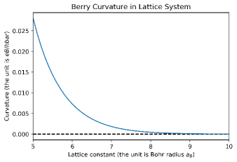
Figure 1: Molecular Berry curvature of the nearest-neighboring nuclei, $F_{nm}^{xy}$ (or, equivalently, $b^{z}_{nm}$), is plotted with respect to the lattice constant. The unit of the vertical and holozontal axis is taken as $ZeB$ and the Bohr radius $a_{B}$, respectively. The number of sites is $N=20\times 20$.

The effective Hamiltonian for the phonons are obtained by considering a small deviation $\bm{u}_{n}$ of the nuclei from its ground state position $\bm{R}_{n}^{0}$; $\bm{R}_{n}=\bm{u}_{n}+\bm{R}_{n}^{0}$. As for the interaction among nuclei, only quadratic terms of $u_{n}^{\alpha}$’s are taken into account. The Berry curvature at the equilibrium atomic positions, i.e., $\left.F_{nm}^{\alpha\beta}\right|_{R=R^{0}}$, is included in the Hamiltonian by the mininal coupling, as in Eq. (3). Hereafter, we omit ‘$R=R^{0}$’ and always take this substitution without notice. Figure 1 shows the numerical evaluation of $F_{nm}^{xy}$ for the nearest-neighbor pair $(n,m)$. a The Berry connection can be expressed by using $\bm{b}_{nm}$ up to the linear order of $u_{n}^{\alpha}$:

$$\bm{a}_{n}= \sum_{m}\frac{1}{2}\bm{b}_{nm}\times\bm{R}_{m}$$

$$= \sum_{m}\frac{1}{2}\bm{b}_{nm}\times\bm{u}_{m}+(\textrm{const.}),$$ (12)

where the constant term can be removed by gauge transformation. Combining the contributions from the external magnetic field and the Berry curvature, the effective vector potential becomes

$$\bm{a}_{n}^{\prime}:= \frac{Ze}{c}\bm{A}(\bm{R}_{n})+\bm{a}_{n}$$

$$= \frac{1}{2}\sum_{m}\bm{b}_{nm}\times(\bm{u}_{m}-\bm{u}_{n}).$$ (13)

In the second line, we used the identity Eq. (11).

The Hamiltonian of the lattice vibration is modified in the exsistence of $\bm{a}^{\prime}_{n}$: the resultant Hamiltonian for our model is given by

$$H_{\textrm{nucl}}= \sum_{n}\Bigl{[}\frac{(\bm{P}_{n}-\bm{a}^{\prime}_{n})^{2}}{2m_{\textrm{nucl}}}+\frac{1}{2}\sum_{m}\bm{u}_{n}^{T}D_{nm}\bm{u}_{m}\Bigr{]}$$ (14a)

$$= \sum_{\bm{k}}\left[\frac{1}{2m_{\textrm{nucl}}}\Pi_{\bm{k}}^{\alpha\dagger}\Pi_{\bm{k}}^{\alpha}+\frac{1}{2}D_{\bm{k}}^{\alpha\beta}u_{\bm{k}}^{\alpha\dagger}u_{\bm{k}}^{\beta}\right],$$ (14b)

where $\Pi_{\bm{k}}:=P_{\bm{k}}-a^{\prime}_{\bm{k}}$ is the momentum under a magnetic field. It is noted that the commutation relationship of $u_{\bm{k}}$ and $\Pi_{\bm{k}}$ is different from that of usual canonical operators: $[u_{\bm{k}}^{\alpha},u_{\bm{q}}^{\beta}]=0$, $[u_{\bm{k}}^{\alpha},\Pi_{\bm{q}}^{\beta}]=i\hbar$, and $[\Pi_{\bm{k}}^{\alpha},\Pi_{\bm{q}}^{\beta}]=i\hbar G_{\bm{k}}^{\alpha\beta}$, where $G_{\bm{k}}^{\alpha\beta}:=\partial_{k\alpha}{a^{\prime}}_{\bm{k}}^{\beta}-\partial_{k\beta}{a^{\prime}}_{\bm{k}}^{\alpha}$. We can see that the effective vector potential plays a role of the Raman interaction. Compared with the original Raman interaction, $\bm{a}^{\prime}_{n}$ does not include $k$-independent constant terms but second-order derivative, so that it vanishes in the $k\to 0$ limit. This is consistent with Eq. (45) of Ref. Qin et al., 2012.

Thermal Hall effect — The effective vector potential $\bm{a}^{\prime}_{n}$ induces the thermal Hall effect of phonons. In this section, we derive the analytic expression for the thermal Hall conductance, $\kappa_{H}$, and numerically estimate it.

The definition of energy current in lattice systems, which we denote $\bm{J}_{E}$, was given by Hardy Hardy (1963) as an operator satisfying local energy conservation law. In addition to the usual Kubo formula, we have to take into account the contribution from the energy magnetization, $\bm{M}_{E}$, defined by $\bm{J}_{E}=\nabla\times\bm{M}_{E}$  Qin et al. (2011). The complete formula for the themal Hall conductance is given by

$$\kappa_{H}^{\textrm{tr}}=\kappa_{H}^{\textrm{Kubo}}+\frac{2M_{E}^{z}}{TV}.$$

The detailed calculation was given by Qin et al. Qin et al. (2012). General formula for the thermal Hall conductance of bosonic particles are:

$$\kappa_{H}^{\textrm{tr}}=-\frac{(\pi k_{B})^{2}T}{3\hbar}Z_{\textrm{ph}}-\frac{1}{T}\int_{0}^{\infty}d\epsilon^{2}~{}\sigma_{xy}(\epsilon)\frac{dn_{B}(\epsilon)}{d\epsilon},$$ (15)

where

$$Z_{\textrm{ph}}:= \sum_{i\in\text{particle bands}}\frac{1}{V}\sum_{\bm{k}\in BZ}\Omega_{\bm{k}i}^{z},$$ (16)

$$\sigma_{xy}(\epsilon):= -\frac{1}{V\hbar}\sum_{\hbar\omega_{\bm{k}i}\leq\epsilon}\Omega_{\bm{k}i}^{z}.$$ (17)

Here, $\omega_{\bm{k}i}$ is the frequency of the phonon of $i$-th mode and $n_{B}(\epsilon)=1/(e^{\beta\epsilon}+1)$ is the Bose distribution. The Berry curvature of phonons is defined as following Zhang et al. (2010); Qin et al. (2012): we define two matrices $\mathcal{A}_{\bm{k}}$ and $\mathcal{B}_{\bm{k}}$ by $\mathcal{A}_{k}=\begin{bmatrix}O&i\hbar\\ -i\hbar&i\hbar G_{\bm{k}}\end{bmatrix}$ and $\mathcal{B}_{k}=\begin{bmatrix}D_{\bm{k}}&O\\ O&1/M\end{bmatrix}$. Here, $\mathcal{A}_{\bm{k}}$ is the commutation relationship of $\xi=\begin{bmatrix}\bm{u}_{\bm{k}}\\ \Pi_{\bm{k}}\end{bmatrix}$, and $\mathcal{B}_{\bm{k}}$ is the bilnear form of the Hamiltonian in $\xi$-basis. From the EoM, the eigenenergy is obtained by diagonalizing $\tilde{H}_{\bm{k}}:=\mathcal{A}_{\bm{k}}\mathcal{B}_{\bm{k}}$. We denote the eigenvectors of $\tilde{H}_{\bm{k}}$ by $|v_{i}\rangle$. Then the Berry connection and curvature are defined by

$$a_{\bm{k}i}^{\alpha}:= -\textrm{Im}~{}\langle v_{i}|\mathcal{B}_{k}\partial_{k\alpha}|v_{i}\rangle,$$ (18a)

$$\Omega_{\bm{k},i}^{z}:= \partial_{kx}a_{\bm{k}i}^{y}-\partial_{ky}a_{\bm{k}i}^{x}.$$ (18b)

The second term in Eq. (15) consists of a summation of Berry curvature over the Brillouin zone and over all the particle bands, $Z_{\textrm{ph}}$. In the previous study, $Z_{\textrm{ph}}$ is supposed to vanish in most cases Qin et al. (2012). For the case of magnonic systems, the summation of Chern number over particle bands is exactly zero Shindou et al. (2013). This can be explained by the fact that the BdG Hamiltonian of the system is adiabatically connected to a trivial matrix, whose Berry curvature is zero. A parallel discussion leads to the conclusion that $Z_{\textrm{ph}}=0$ holds exactly in our model suppl , if we perturb the system to introduce the gap at $\bm{k}=0$ so that the Chern number is well-defined.

On the estimation of $\kappa_{H}$, it is convenient to introduce the continuum approximation. The dynamical matrix and the vector potential of the general Hamiltonian of phonons with Raman-type interaction are given by $D_{\bm{k}}^{\alpha\beta}=\mu_{1}k^{2}\delta^{\alpha\beta}+\mu_{2}k^{\alpha}k^{\beta}$ and ${a^{\prime}}_{\bm{k}}^{\alpha}=\gamma_{1}\partial_{\alpha}\partial_{\beta}\epsilon^{\beta\rho\sigma}M^{\rho}u^{\sigma}+\gamma_{2}\nabla^{2}\epsilon^{\alpha\beta\gamma}M^{\beta}u^{\gamma}$ in Eq. (14b), where $\gamma_{1}$ and $\gamma_{2}$ are coupling constants Qin et al. (2012). The corresponding geometric curvature is $G_{\bm{k}}^{\alpha\beta}=\frac{1}{m_{\textrm{nucl}}}\epsilon^{\alpha\beta\gamma}(-\gamma_{1}k^{\gamma}\bm{k}\cdot\bm{M}+(\gamma_{1}+2\gamma_{2})k^{2}M^{\gamma})$. As long as the temperature is sufficiently low, i.e., the condition $k_{B}T\ll\hbar\omega_{D,i}$ is satisfied for each band $i$ ($\omega_{D,i}:=c_{i}\pi/a$ is the Debye frequency of $i$-th band), the contribution from small $k$ is donimant since the derivative of the Bose distribution function, $dn_{B}(\epsilon)/d\epsilon$, decreases drastically as $\hbar\omega_{\bm{k}i}$ becomes higher. Therefore, at sufficiently low temperature, $\kappa_{H}$ is well estimated by assuming that the continuum approximation is valid over the whole Brillouin zone. Under these conditions, the thermal Hall conductance in two dimension can be calculated by

$$\kappa_{H}^{\textrm{2D}}= -\frac{(\pi k_{B})^{2}T}{3\hbar}Z_{\textrm{ph}}+\frac{\Gamma^{\textrm{2D}}k_{B}^{3}T^{2}}{m_{\textrm{nucl}}\hbar^{2}c_{T}^{2}}\int_{0}^{\infty}dx~{}\frac{x^{3}e^{x}}{(e^{x}-1)^{2}}.$$ (19)

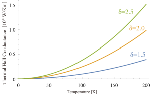
Figure 2: The thermal Hall conductance is plotted with respect to temperature. The blue, orange and green lines correspond to $\delta=$1.5, 2.0 and 2.5, respectively. The used parameters are: $a=6.5a_{B}$, $c_{T}=3000$[m/s] and $B=10$[T].

$\Gamma^{\textrm{2D}}$ is a constant dependent on the ratio of sound speed of the longitudinal and transverse modes, $\delta:=c_{L}/c_{T}$, which is given by

$$\Gamma^{\textrm{2D}}= 2\pi(2\gamma_{2}-\gamma_{1})M^{z}\frac{(\delta-1)^{2}}{\delta(\delta+1)}.$$ (20)

Now, we apply the discussion above to our model. In nonmagnetic insulators, the geometric curvature, $\bm{b}_{nm}$, plays the role of the magnetization $\bm{M}$, and it takes finite value only for nearest-neighbor nuclei. We here denote $\bm{b}_{nm}$ of nearest-neighbor nuclei by $\bm{b}$. The sum over $m$ in Eq. (13) is reduced to the sum over nearest-neighbor nuclei, i.e, $m$ is an integer which satisfies $\bm{R}_{m}^{0}=\bm{R}_{n}^{0}\pm\bm{e}_{x},\bm{R}_{n}^{0}\pm\bm{e}_{y}$ where $\bm{e}_{x}$ ($\bm{e}_{y}$) is the lattice vector for $x$ ($y$)-direction. Assuming $\bm{u}_{n}$ is a slowly-varying parameter of $\bm{R}_{n}$, we expand it by the gradient as $u_{n\pm x(y)}^{\alpha}\simeq u_{n}^{\alpha}\pm a\partial_{x(y)}u_{n}^{\alpha}+\frac{a^{2}}{2}\partial_{x(y)}^{2}u_{n}^{\alpha}$. Then the vector potential (13) becomes

$$\bm{a}^{\prime}(\bm{R})=a^{2}\bm{b}\times\nabla^{2}\bm{u}(\bm{R}).$$ (21)

Therefore the coupling constants are repleced as $\gamma_{1}\to 0$ and $\gamma_{2}M^{z}\to a^{2}b^{z}$.

The dependence on $T$ of $\kappa_{H}^{\textrm{2D}}$ is shown in Figure 2 by using typical parameters. Here, the thermal Hall conductance in two-dimensions is translated into one in three-dimensions by assuming that the thickness of the layer is almost the same as the lattice constant, i.e., the plotted value is $\tilde{\kappa}_{H}:=\kappa_{H}^{\textrm{2D}}/a$. Experimentally, the thermal Hall conductance in magnetic materials is $\kappa_{H}\simeq 10^{-5}$[W/Km] at $T\simeq 5$[K] Strohm et al. (2005); Inyushkin and Taldenkov (2007). Compared to this, $\kappa_{H}$ of our model is much smaller at the same temperature. However, it is detectable enough at higher temperatures. For the experimental realization, Eq. (19) implies that materials with larger overlap integral and smaller transverse sound speed are expected to show larger thermal Hall conductance even without magnetization.

This work was supported by JSPS KAKENHI Grant Nos. JP18H03676, JP18H04222, JP24224009, and JP26103006, ImPACT Program of Council for Science, Technology and Innovation (Cabinet office, Government of Japan), and CREST, JST (Grant No. JPMJCR1874). T.S. was supported by Japan Society for the Promotion of Science through Program for Leading Graduate Schools (MERIT).

References

- Cage et al. (2012) M. E. Cage, K. Klitzing, A. Chang, F. Duncan, M. Haldane, R. B. Laughlin, A. Pruisken, and D. Thouless, The quantum Hall effect (Springer Science & Business Media, 2012).
- Nagaosa et al. (2010) N. Nagaosa, J. Sinova, S. Onoda, A. MacDonald, and N. Ong, Reviews of modern physics 82, 1539 (2010).
- Murakami and Nagaosa (2011) S. Murakami and N. Nagaosa, Comprehensive Semiconductor Science and Technology, Six-Volume Set 1, 222 (2011).
- Xiao et al. (2010) D. Xiao, M.-C. Chang, and Q. Niu, Reviews of modern physics 82, 1959 (2010).
- Onoda et al. (2004) M. Onoda, S. Murakami, and N. Nagaosa, Physical review letters 93, 083901 (2004).
- Katsura et al. (2010) H. Katsura, N. Nagaosa, and P. A. Lee, Physical review letters 104, 066403 (2010).
- Matsumoto and Murakami (2011a) R. Matsumoto and S. Murakami, Physical review letters 106, 197202 (2011a).
- Matsumoto and Murakami (2011b) R. Matsumoto and S. Murakami, Physical Review B 84, 184406 (2011b).
- Hosten and Kwiat (2008) O. Hosten and P. Kwiat, Science 319, 787 (2008).
- Onose et al. (2010) Y. Onose, T. Ideue, H. Katsura, Y. Shiomi, N. Nagaosa, and Y. Tokura, Science 329, 297 (2010).
- Strohm et al. (2005) C. Strohm, G.L.J.A. Rikken, and P. Wyder, Physical review letters 95, 155901 (2005).
- Inyushkin and Taldenkov (2007) A. V. Inyushkin and A. Taldenkov, JETP Letters 86, 379 (2007).
- Sheng et al. (2006) L. Sheng, D.N. Sheng, and C.S. Ting, Physical review letters 96, 155901 (2006).
- Kagan and Maksimov (2008) Y. Kagan and L.A. Maksimov, Physical review letters 100, 145902 (2008).
- Wang and Zhang (2009) J.-S. Wang and L. Zhang, Physical Review B 80, 012301 (2009).
- Zhang et al. (2010) L. Zhang, J. Ren, J.-S. Wang, and B. Li, Physical review letters 105, 225901 (2010).
- Agarwalla et al. (2011) B. K. Agarwalla, L. Zhang, J.-S. Wang, and B. Li, The European Physical Journal B 81, 197 (2011).
- Kronig (1939) R. d. L. Kronig, Physica 6, 33 (1939).
- Qin et al. (2012) T. Qin, J. Zhou, and J. Shi, Physical Review B 86, 104305 (2012).
- Mead (1992) C. A. Mead, Reviews of Modern Physics 64, 51 (1992).
- Ceresoli et al. (2007) D. Ceresoli, R. Marchetti, and E. Tosatti, Physical Review B 75, 161101 (2007).
- Resta (2000) R. Resta, Journal of Physics: Condensed Matter 12, R107 (2000).
- Hardy (1963) R. J. Hardy, Physical Review 132, 168 (1963).
- Qin et al. (2011) T. Qin, Q. Niu, and J. Shi, Physical review letters 107, 236601 (2011).
- Shindou et al. (2013) R. Shindou, R. Matsumoto, S. Murakami, and J.-i. Ohe, Physical Review B 87, 174427 (2013).
- Faddeev and Jackiw (1988) L. Faddeev and R. Jackiw, Physical Review Letters 60, 1692 (1988).
- Raghu and Haldane (2008) S. Raghuand F. D. M. Haldane, Physical Review A 78, 033834 (2008).
- Colpa (1978) J. Colpa, Physica A: Statistical Mechanics and its Applications 93, 327 (1978).
- Berry (2004) M. V. Berry, Czechoslovak journal of physics 54, 1039 (2004).
- (30) See supplemental material at [url will be inserted by publisher] for the derivation of the Berry curvature for general lattice systems (Section I) and an argument for (Section II), which includes Refs. Faddeev and Jackiw, 1988; Raghu and Haldane, 2008; Colpa, 1978; Berry, 2004.