The smectic phase in semiflexible polymer materials:
A large scale Molecular Dynamics study

Abstract

Semiflexible polymers in concentrated lyotropic solution are studied within a bead-spring model by molecular dynamics simulations, focusing on the emergence of a smectic A phase and its properties. We systematically vary the density of the monomeric units for several contour lengths that are taken smaller than the chain persistence length. The difficulties concerning the equilibration of such systems and the choice of appropriate ensemble (constant volume versus constant pressure, where all three linear dimensions of the simulation box can fluctuate independently) are carefully discussed. Using HOOMD-blue on graphics processing units, systems containing more than a million monomeric units are accessible, making it possible to distinguish the order of the phase transitions that occur. While in this model the nematic-smectic transition is continuous, the transition from the smectic phase to a related crystalline structure with true three-dimensional long-range order is clearly of first order. Further, both orientational and positional correlations of monomeric units are studied as well as the order parameters characterizing the nematic, smectic A, and crystalline phases. The analogy between smectic order and one-dimensional harmonic crystals with respect to the behavior of the structure factor is also explored. Finally, the results are put in perspective with pertinent theoretical predictions and possible experiments.

I Introduction

Liquid-crystalline phases of semiflexible polymers are materials with great potential for various applications Krigbaum ; Ciferri ; Donald . The chemical structure of these materials is typically rather complicated and a detailed understanding of structure-properties relations is often rather incomplete. While for liquid crystals formed from small molecules a chemically realistic atomistic molecular modeling has become possible Glaser ; Palermo ; Sidky , the large length scales involved in semiflexible polymers require the use of coarse-grained models Voth . Typical coarse-grained models of semiflexible polymers consist of $N$ “effective monomeric units” with diameter $\sigma$ and distance $\ell_{\rm b}$, evenly placed along the contour of the chain. In such a representation, the contour length, $L$, of the macromolecule is given by $L=(N-1)\ell_{\rm b}$. The chain stiffness, which is responsible for the emergence of liquid crystallinity, is described by the persistence length $\ell_{\rm p}$, which is much larger than the length $\ell_{\rm b}$ of the effective bonds, and can be of the same order as $L$. Previous simulations using such coarse-grained models have been rather successful in the description of the isotropic-nematic transition in lyotropic solutions (assuming an implicit description of the solvent) SEAMKB ; SEAMPVKB ; AMSEKBAN ; popadic:sm:2018 ; popadic:arx:2018 .

For lyotropic solutions of rigid rods ($\ell_{\rm p}/L=\infty$), a subsequent transition to the smectic-A phase has been identified with increasing density in both simulations frenkel:nat:1988 and in experiments Wen . It is possible that smectic phases occur as well in concentrated solutions of less stiff semiflexible polymers ($\ell_{\rm p}\gtrsim L$), but the conditions necessary to find such phases are not understood in sufficient detail Tkach1 ; Tkach2 ; Tkach3 . Simulations so far considered short chains of strongly overlapping beads ($\ell_{\rm b}\ll\sigma$) in order to model slightly flexible rod-like molecules Cinacci ; Schoot ; Schoot3 . While in those studies smectic-A phases were found, the exploration of a bead-spring model of semiflexible chains with $\ell_{\rm b}\approx\sigma$ indicated the emergence of smectic-C order, at least in the two-dimensional case AMSEKB ; AMKB ; KBSEAM . Distorted forms of smectic order were also found under spherical confinement, both in the bulk of the sphere Vega1 ; Vega2 and in thin spherical shells milchev:polymer:2018 ; Khadilkar . Recent simulations AMSEKBAN indicated the occurrence of smectic order in simulations in the bulk at melt densities ($\rho\geq 0.7$) for chains with $\ell_{\rm p}\gg L$, but a detailed study of the smectic phase for this model has not yet been performed.

Such a study is a challenge for molecular dynamics (MD) simulations since the number of smectic layers, $n$, has to be much larger than unity in order to avoid finite-size effects, and the wave length $\Lambda$, characterizing the layered smectic structure, is of the same order as $L$. If the layering occurs in $z$-direction, the simulation box linear dimension $L_{z}$ should be strictly commensurate with $n\Lambda$. However, the precise value of $\Lambda$ is not known beforehand, and also the simulation setup must not suppress statistical fluctuations of $\Lambda$ which are an important ingredient of the problem. As a consequence, one should not use the constant volume (${\cal N}VT$) ensemble (${\cal N}$ is the total number of chains, $V$ is the system volume, and $T$ is the absolute temperature) where the linear dimensions $L_{x}$, $L_{y}$, $L_{z}$ of the simulation box are held fixed. On the other hand, if one uses the constant pressure (${\cal N}PT$) ensemble, one must ensure that also for $L_{z}\gg L_{x},L_{y}$ the transverse linear dimensions $L_{x}$ and $L_{y}$ are sufficiently large to avoid instabilities of the algorithm and possible distortion of the ordering.

From these considerations it is clear that such simulations require the use of an efficient but also versatile simulation software allowing the study of systems containing of the order of million effective monomeric units. Previous efforts using a model with strongly overlapping beads, restricted attention to a single chain length ($N=9$) using ${\cal N}=600$ chains in total Cinacci , or ${\cal N}=4464$ chains with $N=17$ beads Schoot , or ${\cal N}=4608$ chains with $13\leq N\leq 21$ Schoot3 . The aim of the present work, however, is the study of much larger systems, e.g., with up to ${\cal N}N=1694784$ monomeric units to ensure that the results are not affected by systematic finite size effects. Our work did become feasible owing to the availability of the HOOMD-blue software package Anderson ; Glotzer .

The remainder of this manuscript is organized as follows. In Sec. II we shall summarize the methodology to equilibrate the model system and to characterize its liquid-crystalline order. Section III then describes the results while Sec. IV contains our conclusions.

II Model and methods

Our model choice is dictated by the fact that semiflexible polymers in lyotropic solutions may exhibit vastly different conformations in the various phases that are expected to occur. For small enough polymer concentration in the solution, an isotropic phase occurs where the end-to-end vectors of the chains are randomly oriented. For $\ell_{\rm p}\ll L$, these chains have coil-like conformations, whereas in the inverse limit $\ell_{\rm p}\gg L$, they rather resemble flexible rods. In the nematic phase, the chains are always stretched out strongly and have a root mean square end-to-end distance $\left\langle R_{\rm e}^{2}\right\rangle^{1/2}$ not much smaller than $L$ (we disregard here the occurrence of “hairpin“ conformations that are found for $\ell_{\rm p}\ll L$ in the nematic phase close to the isotropic-nematic transition AMSEKBAN ; Vroege ). Being interested in smectic phases with periodicity $\Lambda\sim L$, we focus on the choices $N=8$, $12$, and $16$ here. We choose the same model as in our previous work SEAMKB ; SEAMPVKB ; AMSEKBAN , so that properties of individual chains, etc., in the various phases can be meaningfully compared.

We use here the Kremer-Grest model Grest ; K_G extended by a bending potential to control chain stiffness. The interaction between any pair of beads is purely repulsive and of short range,

$$U_{\rm WCA}(r)=4\epsilon\left[\left(\frac{\sigma}{r}\right)^{12}-\left(\frac{\sigma}{r}\right)^{6}+\frac{1}{4}\right],r\leq r_{c},$$ (1)

where $r$ is the distance between a pair of beads, and $r_{\rm c}\equiv 2^{1/6}\,\sigma$ is the cutoff distance of the potential ($U_{\rm WCA}(r>r_{\rm c})=0$). The parameter $\epsilon$ controls the strength of the potential, and it is chosen as our unit of energy. The bead diameter, $\sigma$, is chosen as the unit of length, and the bead mass, $m$, as the unit of mass.

Further, neighboring beads along a chain interact through the finitely-extensible nonlinear elastic (FENE) potential Grest ; K_G ,

$$U_{\rm FENE}(r)=-0.5kr_{0}^{2}\ln\left[1-\left(\frac{r}{r_{0}}\right)^{2}\right],r<r_{0},$$ (2)

with spring constant $k=30\,\epsilon/\sigma^{2}$. The parameter $r_{0}=1.5\,\sigma$ controls the maximum extension of the spring, and $U_{\rm FENE}(r>r_{0})=\infty$. The distance $\ell_{\rm b}$ between two consecutive beads is $\ell_{\rm b}\approx 0.97\,\sigma$ for the chosen model parameters (the precise value depends slightly on density, temperature and chain stiffness).

The bending potential depends on the angle $\theta_{ijk}$ formed between two consecutive bond vectors $\mathbf{a}_{i}=\mathbf{r}_{j}-\mathbf{r}_{i}$ and $\mathbf{a}_{j}=\mathbf{r}_{k}-\mathbf{r}_{j}$ with $j=i+1$ and $k=j+1$ as

$$U_{\rm bend}(\theta_{ijk})=\kappa[1-\cos(\theta_{ijk})],$$ (3)

where an angle of $\theta_{ijk}=0^{\circ}$ corresponds to three beads in a line. The strength of this potential $\kappa$ is chosen in the range $\kappa=8\,\epsilon$ to $\kappa=128\,\epsilon$.

The persistence length of the polymers, $\ell_{\rm p}$, is defined in terms of $\left\langle\cos(\theta_{ijk})\right\rangle$ Hsu

$$\ell_{\rm p}=-\frac{\ell_{\rm b}}{\ln\left\langle\cos\theta_{ijk}\right\rangle}.$$ (4)

One can show for large $\kappa$ and dilute solutions, where chain interactions can be neglected, that $\ell_{\rm p}\approx\ell_{\rm b}\kappa/(k_{\rm B}T)$ (with Boltzmann’s constant $k_{\rm B}$ and temperature $T$). In concentrated solutions or melts with liquid crystalline order, however, the actual persistence length found from Eq. (4) can be significantly enhanced in comparison with this estimate for the “bare” persistence length AMSEKBAN .

This model has been studied by MD simulations Tildesley ; Rapaport . Both ${\cal N}VT$ and ${\cal N}PT$ ensembles have been used, employing a time step $\Delta t=0.002\,t_{\rm MD}$, with intrinsic time unit of MD, $t_{\rm MD}=\sqrt{m\sigma^{2}/\epsilon}$. In the ${\cal N}VT$ simulations, temperature was controlled through the standard Langevin thermostat Grest ; K_G as in our previous work SEAMKB ; SEAMPVKB ; AMSEKBAN . For the ${\cal N}PT$ simulations we use a Martyna-Tuckerman-Tobias-Klein barostat Martyna ; Klein , where the equations of motion are time reversible and leave the phase space measure invariant. The coupling constants for the thermostat and barostat were chosen as $t_{T}=0.5$ and $t_{P}=1.0$, respectively. As emphasized already in the introduction, because of the necessity of very large system sizes, this work becomes possible only due to the availability of HOOMD-blue Anderson ; Glotzer .

The ${\cal N}PT$ ensemble was chosen in a variant where all linear dimensions of the box were identical, so a cubic $L_{x}\times L_{y}\times L_{z}$ shape of the simulation box was enforced, as well as in a variant where the linear dimensions $L_{x}$, $L_{y}$, and $L_{z}$ were allowed to fluctuate independently, employing hence a box of rectangular slab shape. Periodic boundary conditions in all directions were used throughout. The choice of a cubic box in the ${\cal N}VT$ ensemble is appropriate for the system in its isotropic phase, but becomes questionable in the liquid-crystalline phases. This is explicitly seen when we record the pressure tensor $P^{\alpha\beta}$ and its fluctuations ($\alpha,\beta=x,y,z$). The instantaneous pressure is found from the Virial expression Tildesley

$$P^{\alpha,\beta}=\rho k_{\rm B}T\delta^{\alpha,\beta}+\frac{1}{3V}\sum_{i}r_{i}^{\alpha}F_{\rm tot}^{\beta}(\mathbf{r}_{i})$$ (5)

where the sum extends over all beads in the system, the density $\rho$ is given by $\rho\equiv N{\cal N}/V$, and $\mathbf{F}_{\rm tot}(\mathbf{r}_{i})$ is the total force acting on bead $i$ at position $\mathbf{r}_{i}$ due to the potentials Eqs.(1)-(3).

We initialize the chains as straight rods along the $z$-axis, and then arrange the chains on a square lattice (or, alternatively, on a triangular lattice). The lattice spacing is chosen such that the desired density $\rho$ is reached, and $n$ of these layers of stretched chains are then put on top of each other. The choice of the proper value of $n$ (or $L_{z}$) is not obvious a priori, because the precise value of the smectic period, $\Lambda$, that eventually develops is not known in beforehand. It is necessary to make sure that a slightly incorrect choice of $n$ does not prevent the approach towards the correct equilibrium state. For example, the choice $N=8$, ${\cal N}=101568$ and $L_{x}=L_{y}=L_{z}=100$, leads to a density of $\rho=0.8125$. If one tries to equilibrate such a system, initialized with a regular arrangement comprising $n=12$ smectic layers, one obtains a strongly distorted smectic structure. Choosing $L_{z}$ slightly larger, namely $L_{z}=104$, then $13$ layers would fit better than only $12$ layers, and indeed we observe a transition from $n=12$ to $n=13$ during the run, Fig. 1.

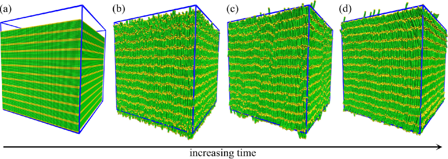
Figure 1: Formation of an ordered phase of semiflexible polymers with $N=8$, $\kappa=96$, ${\cal N}=101568$ in a $98.06\times 98.06\times 104$ box, with $\rho=0.8125$ at $k_{\rm B}T=0.5$. The initial state (a) is a regular arrangement of 12 layers of straight chains with some extra volume on top. At $t=100$ (b), this density inhomogeneity is removed but only local disorder in the $n=12$ layers has appeared. At $t=1400$ (c), however, there is a local defect in the layering, a new $13^{th}$ layer starts to form and a stable 13 layers persist as a final structure. The last snapshot refers to $t=20000$ (d).

The system shown in Fig. 1 has been initialized using a square lattice arrangement of chains in the $xy$-plane, stretched out along the $z$-axis. This configuration is clearly not similar to the crystalline ground state of our model, since a regular packing of rigid rods would rather result in a triangular lattice structure in the cross-sectional $xy$-plane. In order to test for a possible bias in our results, due to the choice of the initial state, we have also carried out runs with a triangular lattice arrangement of rod-like polymers (and choosing then $L_{x}/L_{y}=2/\sqrt{3}$ so that the triangular lattice arrangement is compatible with the periodic boundary condition). We have found that the memory of the initial crystalline chain arrangement is quickly lost for the densities of interest. The initial layering does not create an undue bias either. We have tested this fact by creating artificial states with hexagonal order in the $xy$- plane but disorder in the $z$-coordinates of the center of mass positions of the stretched out polymers. Hence, it appears that for the densities of interest the resulting nematic or smectic structures are developing with the proper order irrespective of this initial disorder. Alternatively, one could also attempt to produce ordered phases starting from fully disordered isotropic chain configurations. However, this task is quite challenging since the growth of ordered domains is a rather slow process to be convenient for simulations.

The time evolution in Fig. 1 shows that the extra volume for $n=12$ layers in a $98\times 98\times 104$ box is rapidly filled at first, and then large-scale defects in the structure form by which the system is able to create an extra layer and form the more stable arrangement with $n=13$ layers. However, the final snapshot clearly reveals that for the chosen conditions a small mechanical deformation (“buckling”) is still present: this can be avoided only by using a ${\cal N}PT$ rather than ${\cal N}VT$ simulations.

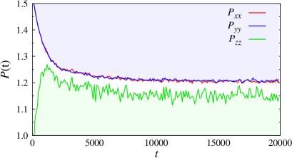
Figure 2: Time evolution of pressure tensor components parallel ($P_{zz}$) and perpendicular ($P_{xx},P_{yy}$) to the nematic director, for the system $N=8$, ${\cal N}=101568$, $\kappa=16$, $L_{x}=L_{y}=98.06$, $L_{z}=104$, and $k_{\rm B}T=1.0$.

This conclusion is enforced by following the time evolution of the pressure tensor components, Fig. 2. It is seen that a time of order $10^{4}\,t_{\rm MD}$ is necessary to relax the system until the individual pressure components become independent of time but a systematic difference $\delta P\equiv P_{zz}-(P_{xx}+P_{yy})/2$ of order $0.05$ remains when we work in the ${\cal N}VT$ ensemble.

$L_{x}$	$L_{y}$	$L_{z}$	$P_{xx}$	$P_{yy}$	$P_{zz}$	$\rho$	$S$	$\left\langle R_{\rm e}^{2}\right\rangle$	$\left\langle R_{{\rm e},z}^{2}\right\rangle$	$\left\langle R_{{\rm e},\perp}^{2}\right\rangle$	$\langle\ell_{\rm b}^{2}\rangle$
134.06	134.06	134.06	1.285	1.285	1.269	0.680	0.913	203.5	197.5	5.95	0.938
134.1	134.1	134.1	1.282	1.283	1.266	0.679	0.912	203.5	197.5	5.95	0.938
135.7	135.6	131.0	1.280	1.283	1.282	0.679	0.912	203.4	197.5	5.95	0.938
108.1	108.1	204.3	1.285	1.285	1.281	0.680	0.911	203.4	197.3	6.18	0.938

Table 1: Simulation results for $N=16$ and $\kappa=64$. Linear dimensions of the simulation box $L_{x}$, $L_{y}$, and $L_{z}$. Diagonal components of the pressure tensor, $P_{xx}$, $P_{yy}$, and $P_{zz}$. Monomer density, $\rho$, nematic order parameter, $S$, mean-square end-to-end distance, $\left\langle R_{\rm e}^{2}\right\rangle$, and its $z$-component, $\left\langle R_{{\rm e},z}^{2}\right\rangle$, as well as its transverse component, $\left\langle R_{{\rm e},\perp}^{2}\right\rangle$. Mean-square bond length, $\left\langle\ell_{\rm b}^{2}\right\rangle$.

Already in the nematic phase such systematic differences start to show up as demonstrated in Table 1, cf. Ref. AMSEKBAN . The results are for the case $N=16$, $\kappa=64$ at $k_{\rm B}T=1.0$. The first line uses the ${\cal N}VT$ ensemble with a cubic box. Note that $P_{zz}$ is slightly smaller than $P_{xx}\approx P_{yy}$. The second line shows ${\cal N}PT$ results for the choice $P=1.28$ but allowing only uniform volume fluctuations. The initial conformation was taken here from the constant volume ensemble. The third line shows also ${\cal N}PT$ results for $P=1.28$, but now $L_{x}$, $L_{y}$, and $L_{z}$ can fluctuate independently of one another. Note that now the desired result $P_{xx}\approx P_{yy}\approx P_{zz}$ holds within the statistical error (which here is about $10^{-3}$). The final line shows ${\cal N}VT$ results for an elongated box, linear dimensions taken from an equilibrated configuration in the ${\cal N}PT$ ensemble (for the choice $P=1.28$). Clearly, the uniaxial symmetry of the nematic order with the director along the $z$-axis is incompatible with a cubic box, so independent fluctuations of $L_{x}$, $L_{y}$ and $L_{z}$ in the ${\cal N}PT$ ensemble are needed. Gratifyingly, in the nematic phase the results for the nematic order parameter $S$ as well as the chain linear dimensions $\left\langle R_{{\rm e},z}^{2}\right\rangle$ and $\left\langle R_{{\rm e},\bot}^{2}\right\rangle$ in the ${\cal N}VT$ ensemble agree with their counterparts in the ${\cal N}PT$ ensemble. Therefore it is useful to start with a study in the ${\cal N}VT$ ensemble (which is computationally somewhat easier) to get a first orientation of the present problem.

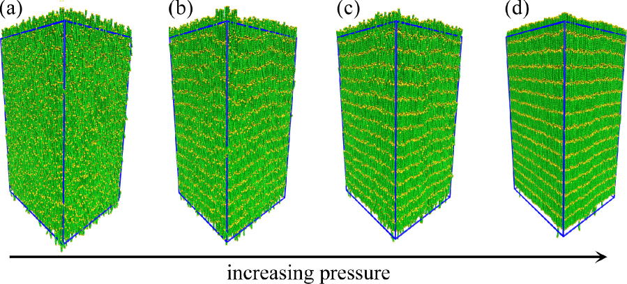
Figure 3: Snapshots of a system with ${\cal N}=89600$ chains of length $N=12$ at $k_{\rm B}T=0.5$ for $\kappa=64$ and four different pressures (a) $P=0.6$, (b) $P=0.7$, (c) $P=0.8$, and (d) $P=0.9$, as indicated. Case (a) shows a resulting nematic state, cases (b), (c) are typical smectic states, while case (d) refers to a somewhat disordered crystal. Monomers are shown in green, apart from the chain ends which are shown in yellow and the edges of the simulation box are indicated by straight blue lines. In order to reduce finite size effects, the linear dimension of the simulation box in the $z$-direction was chosen about twice as large as in the $x$, $y$-directions.

Fig. 3, as a preview of results whose precise analysis will follow below, shows typical snapshot pictures of chain with $N=12$, $\kappa=64$ at $k_{\rm B}T=0.5$ for the (a) nematic, (b, c) smectic, and (d) crystalline phases of this model, as obtained in the ${\cal N}PT$ ensemble when all linear dimensions $L_{x}$, $L_{y}$, and $L_{z}$ are allowed to fluctuate independently.

III Results

III.1 Phase diagrams and chain center of mass distribution functions

We first focus on a system with $N=8$, $\kappa=16$, ${\cal N}=101568$ at $k_{\rm B}T=0.5$. While previous work on the isotropic-nematic transition SEAMKB ; SEAMPVKB ; AMSEKBAN did always choose $N\geq 16$ (and $k_{\rm B}T=1.0$), we deliberately study here shorter chains first, since then finite-size effects associated with the small number of smectic layers are expected to be less relevant. But for $N=8$ and $k_{\rm B}T=1.0$ the isotropic-nematic transition is shifted to a high density already so that a possible smectic phase would be hard to distinguish from a crystalline phase, which we expect at densities in the order of $\rho=1.0$ (i.e. when the monomers effectively “touch”). Figure. 4a, shows the nematic order parameter $S$ (see definition below) as a function of $\rho$ at $k_{\rm B}T=0.5$, demonstrating that the phases are well separated from each other at the lower temperature; the isotropic-nematic transition occurs at density $\rho\approx 0.59$ while the nematic-smectic transition takes place at density $\rho\approx 0.74$. For densities $\rho\gtrsim 0.81$ the semiflexible polymers obtain hexatic (or even crystalline) order.

The nematic order parameter $S$ is defined as the largest eigenvalue $\lambda_{3}$ of the tensor $Q^{\alpha\beta}$, characterizing the average bond orientational order of the chains; denoting $\mathbf{u}_{ij}$ a unit vector along the bond vector $\mathbf{a}_{ij}$, referring to effective monomer $i$ of chain $j$, we have

$$Q^{\alpha\beta}=\frac{1}{2}\left(\left\langle 3u_{ij}^{\alpha}u_{ij}^{\beta}\right\rangle-\delta^{\alpha\beta}\right),$$ (6)

where the average $\langle\ldots\rangle$ is both a temporal average and an average over all the ${\cal N}(N-1)$ bonds in the system. In general, the tensor $Q^{\alpha\beta}$ has three eigenvalues $\lambda_{3}>\lambda_{2}>\lambda_{1}$, but in the nematic phase the biaxiality $B=(\lambda_{2}-\lambda_{1})/2$ is zero, and since $Q^{\alpha\beta}$ is traceless, we must then have $\lambda_{2}=\lambda_{1}=-S/2$. We have computed $B$ as a check, and find indeed $B\approx 0$ in the nematic phase (within statistical error). Slightly nonzero values of $B$ occur in the smectic phase, however. This slight increase of $B$ may indicate minor banana-shape distortion of the chains, resulting from a misfit of the smectic layer in the simulation box. This preliminary identification of the nature of the smectic phase (as well as the observation of chain distortion) is suggested by snapshot pictures, similar to Figs. 1,3.

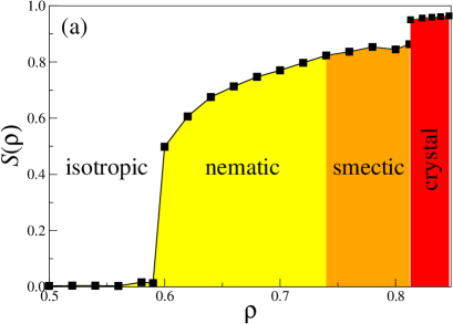
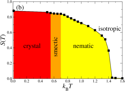
Figure 4: (a) Nematic order parameter, $S$, vs density, $\rho$, in a system with $N=8$, $\kappa=16$, $k_{\rm B}T=0.5$ and ${\cal N}=101568$. Simulations have been conducted in the ${\cal N}VT$ ensemble, using a simulation box with $L_{x}=L_{y}$, and $L_{z}=100$. The lateral linear dimensions, $L_{x}$ and $L_{y}$, were adjusted such that the shown values of $\rho$ resulted. (b) Nematic order parameter, $S$, plotted vs $k_{\rm B}T$, in the same system as panel (a), using a cubic simulation box with $L_{x}=L_{y}=L_{z}=100$ and $\rho=0.812544$.

An alternative description of the global phase diagram is possible by retaining a density $\rho=0.812544$ and varying the temperature, $T$, as shown in Fig. 4b. It is found that the distortion of the smectic phase (measured by a small but definitely nonzero biaxiality $B$) persists up to the transition to the nematic phase at about $k_{\rm B}T=0.69$. This transition does not involve a discontinuity in $S$, suggesting (as Fig. 4a does) that the nematic-smectic A transition is continuous.

In order to identify smectic phases more precisely, we have studied the correlation functions between the center of mass positions of the chains, both along the $z$-direction, $g_{\parallel}(\Delta z)$, and in the radial direction perpendicular to the $z$-axis, $g_{\perp}(\Delta r_{\perp})$. Here, we denote the components of the distance vector between the center of mass positions of two chains as $(\Delta x,\Delta y,\Delta z)$ with $\Delta r_{\perp}=\sqrt{(\Delta x)^{2}+(\Delta y)^{2}}$. Figures 5 and 6 show the data for two selected cases, revealing that the onset of smectic order shows up by means of periodic modulation of $g_{\parallel}(\Delta z)$. For the case of $N=8$, $\kappa=16$, $k_{\rm B}T=0.5$ (Fig. 5), the modulation sets in at $\rho\approx 0.77$ with a wave length of $\Lambda=7.9$. This wavelength slightly exceeds the minimum length $\sqrt{\left\langle R_{{\rm e},z}^{2}\right\rangle}+\sigma\approx 7.6$, needed for a smectic structure. Note that at each chain’s end $\sigma/2$ has to be added to account for the excluded volume of the end monomers, and $\sqrt{\left\langle R_{{\rm e},z}^{2}\right\rangle}\approx 6.6<L\approx 6.8$ due to the slight tilt of the chains in the smectic order. Thus there is some extra free volume gained for the chain ends in the smectic structure, and the resulting entropy gain is in fact responsible for stabilizing smectic rather than nematic order Tkach3 ; Cinacci .

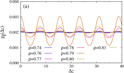
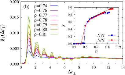
Figure 5: (a) Distribution function $g_{\parallel}(\Delta z)$ of the distances of the centers of mass of the chains in $z$-direction for the case $N=8$, $\kappa=16$, ${\cal N}=101568$, $k_{\rm B}T=0.5$, plotted vs $\Delta z$ for 7 densities. Data from ${\cal N}VT$ simulations in a cubic simulation box. (b) Radial distribution function $g_{\perp}$ of the chains center of mass positions for the same system as in (a). The inset shows the corresponding variation of $S$ with density in the ${\cal N}VT$ and ${\cal N}PT$ ensemble.

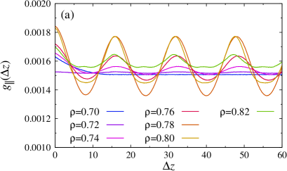
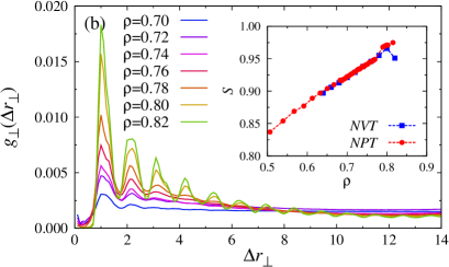
Figure 6: (a) Distribution function $g_{\parallel}(\Delta z)$ of the distances of the centers of mass in the $z$-direction for the case $N=16$, $\kappa=64$, ${\cal N}=101568$, $k_{\rm B}T=1.0$, plotted vs $\Delta z$ for 7 densities. Data from ${\cal N}VT$ simulations in a cubic simulation box. (b) Radial distribution function $g_{\perp}$ of the chain center of mass positions for the same system as in (a). The inset shows the corresponding variation of $S$ with density in the ${\cal N}VT$ and ${\cal N}PT$ ensemble.

However, while for $\rho=0.76$ the box linear dimension is about $L_{x}=L_{y}=L_{z}=102.25$, and hence 13 periods do fit into the box, for $\rho=0.80$ the linear dimension is only about $100.52$, implying a significant distortion of the smectic layering with the “natural” period $\Lambda$ as far as neither 12 nor 13 periods would fit nicely into the box. The same conclusion emerges from $g_{\perp}(\Delta r_{\perp})$, Fig. 5b. A pronounced radial correlation of the center of mass positions does develop with density in the same range where the periodic modulation in the $z$-direction is present. But it is also seen that a weak much larger periodicity is superimposed which is likely a consequence of the elastic deformation caused by the incommensurability of the smectic layering with the linear dimension of the box. Due to this misfit (and pressure anisotropies, similar to Fig. 2) there is a small systematic error in the value of the order parameter $S$ as a comparison with the ${\cal N}PT$ results shows.

These incommensurablity effects are even more pronounced for longer chains where less smectic layers fit in a simulation box of similar size. In any case, Fig. 5 suggests a kind of long-range order in the direction of the smectic modulation (the $z$-axis) but short-range order in the perpendicular direction, as expected for a smectic which is still fluid.

In the second example ($N=16$, $\kappa=64$, $k_{\rm B}T=1.0$), the onset of smectic order is clearly recognized for $\rho=0.74$, Fig. 6a, where a periodicity of $g_{\parallel}(\Delta z)$ with $\Lambda\approx 16$ is apparent. This periodicity becomes more pronounced for $\rho=0.76$ and $\rho=0.78$, as is obvious from the increase of the amplitude of the periodic variation. However, for $\rho\geq 0.8$ the amplitude starts to decrease again and the comparison with the ${\cal N}PT$ reveals for $S(\rho)$ a systematic error again. This effect is due to an increasing misfit of smectic order with growing density: for $\rho=0.74$ the linear dimensions of a cubic box are $L_{x}=L_{y}=L_{z}=130.33$ while for $\rho=0.8$ we have $L_{x}=L_{y}=L_{z}=126.99$. So if the smectic order has a “natural” periodicity $\Lambda$ that fits well in the box with $L_{z}=130.33$, it clearly will fit less well in the box with $L_{z}=126.99$. Again the fact that the center of mass correlation in the transverse direction (Fig.6b) exhibits pronounced short-range order, but no long-range order, provides strong evidence that one deals here with a smectic yet not a crystalline phase (see also discussion in Sec. III.2 below).

It is remarkable that despite the significant distortion of the smectic structure the resulting values for the order parameter $S(\rho)$ in Fig. 5a differ only marginally from those shown in Fig. 4 for the $L_{x}=L_{y}=100$ geometry. But it is clear that also in this case there is an inevitable misfit of the natural periodicity of the smectic structure. To obtain more reliable data, the choice of ${\cal N}PT$ simulations where $L_{x}$, $L_{y}$, and $L_{z}$ are allowed to fluctuate independently is indispensable.

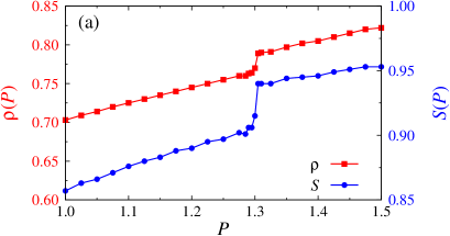
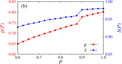
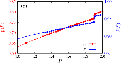
Figure 7: (a) Density, $\rho$, vs pressure, $P$, isotherms for a few representative cases: (a) $N=12$, $\kappa=16$, $k_{\rm B}T=0.5$, (b) $N=12$, $\kappa=64$, $k_{\rm B}T=0.5$, (c) $N=12$, $\kappa=64$, $k_{\rm B}T=1.0$, and (d) $N=16$, $\kappa=64$, $k_{\rm B}T=1.0$. The right axis in these figures show the nematic order parameter $S$ vs $P$.

One of the clear advantages of the ${\cal N}PT$ ensemble emerges when we study the equation of state of the system: plotting the isotherm density against pressure, a first order transition between phases with a different character of the order shows up via two distinct branches separated by a density jump. In the ${\cal N}VT$ ensemble, the region of the density jump would correspond to a two-phase coexistence region, and often such regions are hard to analyze because of finite-size effects caused by interfaces. Indeed, Fig. 7 reveals that such a first order transition does occur in our system at high densities, typically in a region of densities $0.76\leq\rho\leq 0.80$ (cf. Fig. 7). The nematic order parameter $S$ in this region then always exceeds $S=0.9$ markedly, and shows also a jump (cf. Fig. 7). From various analyses (such as those in Figs. 5 and 6) we have identified the phase at densities that are somewhat smaller than the density of this first order transition as smectic phases. The high density phase can be identified as a crystalline phase. In the next subsection, we shall discuss order parameters that are suitable to characterize the order both of the smectic phase and of even more ordered phases such as hexatic liquid crystals and truly crystalline phases.

III.2 Order parameters

From Fig. 7 it is evident that neither the density, $\rho$, nor the nematic order parameter, $S$, show any discontinuity at the nematic-smectic transition. This conclusion is corroborated by a study of the nematic order of the full chains Tortora rather than the bonds. We define a chain order parameter in analogy with Eq. (6) simply in terms of the mean square end-to-end distance components of the chains by

$$S_{c}=\frac{3}{2}\frac{\left\langle R_{{\rm e},z}^{2}\right\rangle}{\left\langle R_{\rm e}^{2}\right\rangle}-\frac{1}{2}$$ (7)

Fig. 8 compares $S_{c}$ and $S$, plotted vs density, for two typical cases. Also the typical inclination of the chains relative to the director, measured via $I_{c}\equiv\sqrt{\left\langle R_{{\rm e},xy}^{2}\right\rangle/\left\langle R_{\rm e}^{2}\right\rangle}$ with $\left\langle R_{{\rm e},xy}^{2}\right\rangle=(\left\langle R_{{\rm e},x}^{2}\right\rangle+\left\langle R_{{\rm e},y}^{2}\right\rangle)/2$, is shown. This inclination is typically of the order of $0.1$ to $0.25$, corresponding to misalignments of $5^{\circ}$ to $15^{\circ}$, and it is probably due to long wavelength collective buckling fluctuations of the nematic alignment of the chains.

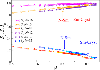
Figure 8: Chain order parameter $S_{c}$, Eq. (7), bond order parameter $S$, Eq. (6), and typical chain inclination $I_{c}\equiv\sqrt{\left\langle R_{{\rm e},xy}^{2}\right\rangle/\left\langle R_{\rm e}^{2}\right\rangle}$ plotted vs density, $\rho$. Data for $N=12$ and $N=16$ for the case $k_{\rm B}T=1.0,\kappa=64$ are included. Arrows indicate the location of the nematic-smectic transition, while the (first order) smectic-crystal transition in this plot shows up as a density gap, representing two-phase coexistence. All data were computed from runs in the ${\cal N}PT$ ensemble. Note that in the smectic region $\left\langle R_{\rm e}^{2}\right\rangle$ is only marginally smaller than the results for a strictly linearly stretched chain (e.g., for $N=12$, $\rho\approx 0.76$, we find $\left\langle R_{\rm e}^{2}\right\rangle/L^{2}\approx 0.97$).

In order to characterize the smectic order quantitatively, and also locate more precisely the nematic-smectic phase boundary, we introduce an additional order parameter $\tau$ that describes the periodic density modulation occurring in the smectic phase. In an ideal smectic A phase the local monomer density along the $z$-axis, perpendicular to the layers and coinciding with the nematic director, is proportional to deGennes :

$$\rho(z)\propto\cos\left(\frac{2\pi}{\Lambda}z+\varphi\right),$$ (8)

where $\Lambda$ is the period of the smectic modulation, and $\varphi$ is a phase (which is of no interest here). Eq. (8) only holds in the smectic A phase near the nematic-smectic transition, and neither $\Lambda$ nor $\varphi$ are known beforehand. Deeper in the smectic phase higher harmonics need to be added to Eq. (8). In order to determine $\Lambda$ in the general case, it is appropriate to consider the structure factor $S(\mathbf{q})$, with wave vector $\mathbf{q}$ oriented parallel to the $z$-axis,

$$S(q_{z})=\frac{1}{{\cal N}N}\left\langle\left|\sum_{j}\exp(iq_{z}z_{j})\right|^{2}\right\rangle,$$ (9)

where the sum runs over all monomers at positions $\mathbf{r}_{j}=(x_{j},y_{j},z_{j})$ in the system. In the smectic phase, we expect that $S(q_{z})$ must have a rather sharp peak at $q_{z}=2\pi/\Lambda$ (see Fig. 12 below). The smectic order parameter, $\tau$, is then defined as the amplitude of the largest peak of $S(q_{z})$. Alternatively, one can compute the area of $S(q_{z})$ underneath the (first) Bragg peak at $q_{z}=2\pi/\Lambda$, and take $\tau$ as the square root of this area.

Eq. (9) works well when one deals with relatively small systems (a few thousand short chains were used in Refs. 19; 20). However, for the large systems studied here (of the order of $100000$ chains) one finds often a rather erratic behavior of the resulting order parameter when plotted vs density or pressure. This happens because in such large systems the smectic order that develops is nonuniform due to defects (resembling “spiral dislocations”, Fig. 9). Only by long annealing it is sometimes possible to heal out these defects and obtain uniform long range order throughout the whole simulation box, as shown in Fig. 9. To avoid the extreme investment of computer resources needed to achieve such annealing, we have found it more convenient to extend the summation over the monomer coordinates in Eq. (9) not over the full box, but only over subboxes $l\times l\times L_{z}$ with $l=5$ or $l=10$, respectively. We have checked that in the smectic phase the dependence of $\tau$ on $l$ is very weak, and that $\tau$ roughly agrees with the result extracted from Eqs. (9) when uniform order is achieved in the system. However, the drawback of this method is that in the nematic phase the resulting $\tau$ is also nonzero. Such “finite size tails” of $\tau$ in the nematic phase are familiar from similar findings at second-order phase transitions KBDWH .

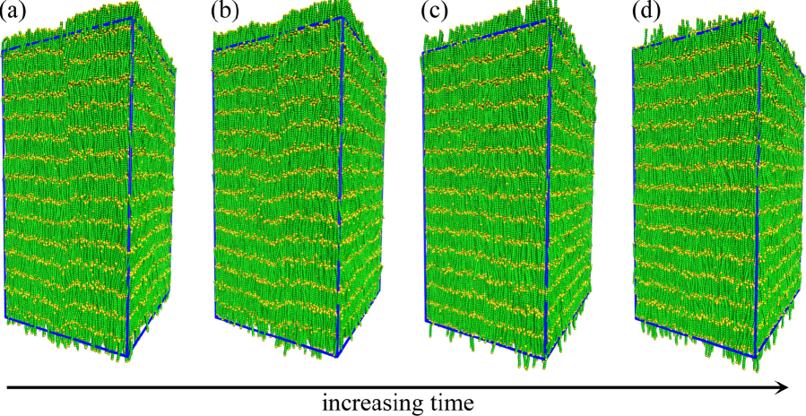
Figure 9: Snapshot pictures of the configuration of a system with $N=12$, ${\cal N}=89600$, $\kappa=64$, $k_{\rm B}T=1.0$, and $P=2.225$ at time (a) $t=1.6\times 10^{4}$, (b) $t=1.8\times 10^{4}$, (c) $t=2\times 10^{4}$, and (d) $2.2\times 10^{4}$, as indicated. Chain ends are shown in yellow while the remaining monomers of the chains are shown in green. The simulation box is indicated by blue lines. Note that in cases (a) and (b) a spiral dislocation defect is present, but has disappeared in panels (c) and (d). Comparing the frames (c) and (d), one detects a slight difference in the phase of the periodic ordering, $\varphi$, Eq. (8). Due to the random diffusive motion of the chains the phase is not fixed in space in the laboratory system, as it should be, since the smectic phase is still a fluid and not a solid.

Figure 10 gives a plot of the period $\Lambda$ (normalized by $L+\sigma$) versus density for a few typical cases. It is seen that $\Lambda$ exceeds the estimate $L+\sigma$ slightly, indicating that the chain ends require more space than this simple estimate suggests. The period seems to depend only weakly on $\rho$, $T$ and $\kappa$.

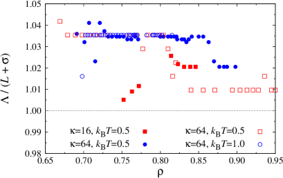
Figure 10: Period $\Lambda$ of the smectic order parameter vs density, $\rho$, for chains with length $N=8$ (filled symbols) and $N=16$ (open symbols), for various stiffnesses, $\kappa$, and temperatures, $T$, as indicated.

Figure 11 shows the typical behavior of the smectic order parameter extracted from our simulations, revealing a seemingly continuous transition from the nematic phase. (Because of equilibration problems and finite size effects we did not attempt to characterize the transition more precisely.) Theoretically, it is well accepted that true solid-like long range order in only one dimension is not possible Landau ; deGennes2 . As these systems are at their lower critical dimension, fluctuations prevent true long range translational order Caille . Also in experiments, however, the observed behavior is hardly distinguishable from a second order transition Safinya .

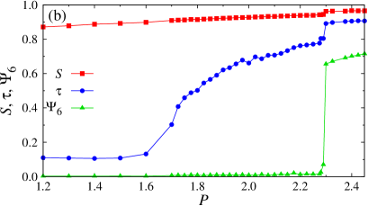
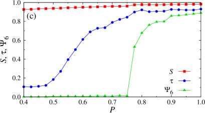
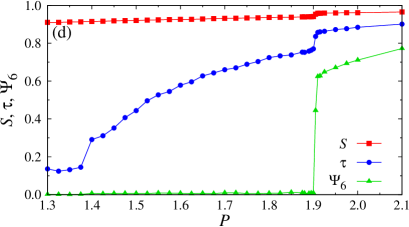
Figure 11: Variation of the order parameters $S$, $\tau$ and $\Psi_{6}$ with pressure, $P$, for a few typical cases: (a) $N=8$, $\kappa=16$, $k_{\rm B}T=0.5$, (b) $N=12$, $\kappa=64$, $k_{\rm B}T=1.0$, (c) $N=16$, $\kappa=64$, $k_{\rm B}T=0.5$, (d) $N=16$, $\kappa=64$, $k_{\rm B}T=1.0$. Curves are intended to guide the eyes only.

As the density is increased further, the chains need to pack more tightly and eventually crystalline order emerges in the lateral direction. We quantify this structuring by considering the transverse order of the center of mass positions $\mathbf{r}^{\rm CM}=(\mathbf{r}^{\rm CM}_{\perp,\alpha},z^{\rm CM}_{\alpha})$ of the chains in the individual smectic layers ($\alpha$ labels the chains in a selected smectic layer). We ask whether these coordinates $\{\mathbf{r}^{\rm CM}_{\perp,\alpha}\}$ form a triangular lattice order, and therefore record the bond order parameter

$$\Psi_{6\alpha}=\frac{1}{n_{\beta}}\sum_{\beta=1}^{n_{\beta}}\exp(i6\phi_{\alpha\beta}),$$ (10)

where the sum over $\beta$ runs over the $n_{\beta}$ nearest neighbors of $\alpha$ ($n_{\beta}=6$ in the case of a perfect lattice) and $\phi_{\alpha\beta}$ is the angle between the vector $\mathbf{r}^{\rm CM}_{\perp,\beta}-\mathbf{r}^{\rm CM}_{\perp,\alpha}$ and the $x$-axis. We average $\Psi_{6\alpha}$ over all chains $\{\alpha\}$ in a layer and over all layers.

The $\Psi_{6}$ analysis can also be extended to densities in the nematic phase where the system is arbitrarily divided into layers of thickness $L$. However, already in the smectic phase the average $\Psi_{6}=M^{-1}|\sum_{\alpha}\Psi_{6\alpha}|$ vanishes in the limit when the number of chains per (smectic) layer, $M$, tends to infinity, whereas in the crystal phase the average $\Psi_{6}$ is clearly nonzero. In the smectic A phase, the correlation function of $\Psi_{6}$ is expected to decay exponentially with distance $r_{\perp}$. If a quasi-two-dimensional hexatic phase occurs, where the lateral order of subsequent smectic layers is decoupled, a power-law decay with $r_{\perp}$ is expected. However, due to finite size effects and large statistical fluctuations, these correlations are difficult to study, and this calculation has not been attempted here yet.

In Fig. 11 we have plotted $\Psi_{6}$ vs pressure for selected systems. In the smectic and nematic phase, $\Psi_{6}$ is essentially zero. At the transition pressure of the crystalline phase, $\Psi_{6}$ abruptly jumps to values in the range $0.7\leq\Psi_{6}\leq 0.9$ and increases with $P$ for the cases considered. The small finite values of $\Psi_{6}$ that we find in the smectic phase are clearly a fluctuation effect because we expect then a distribution $P(\Psi_{6})\propto\Psi_{6}\exp(-\Psi_{6}^{2}M/2\chi_{6})$ in the smectic phase with $\chi_{6}$ being an appropriate response function. The strong positional correlation between the center of mass positions in the transverse direction (Figs.5 and 6) in these rather dense fluid phases imply also rather strong bond-orientational correlations. These correlations lead to large values of $\chi_{6}$, reflected in the fluctuations seen in $\Psi_{6}$ in the smectic phase, but absent in the nematic phase.

III.3 The scattering function $S(q_{z})$ in the smectic-A phase

We have already mentioned that the quasi-one-dimensional periodic order of smectic layers is not a true long range order like in a crystal, since the system is somewhat unstable against thermal fluctuations deGennes2 ; Caille ; Safinya ; Nelson ; Shalaginov . This conclusion is drawn by analogy to the well known problem that one-dimensional “crystals” are always disordered at nonzero temperature Landau . Here, we explore this analogy in more detail.

Figure 12: (a) Structure factor $S(q)$ for the system with $N=12$, $\kappa=64$, $k_{\rm B}T=1.0$ and pressure $P=2.225$ plotted vs $q\equiv q_{z}$. The inset shows the same data on a logarithmic ordinate scale. (b) Plot of $S(q)$ vs $q$, computed from Eq. (11), taking $n=14$ and $\Lambda=11.97$ from panel (a). (c) Plot of $S(q)$ vs $q$, according to Eq. (12) [normalized by $S(q_{1})$], taking the same $\Lambda$ as in panels (a) and (b), and the choice $\delta^{2}=0.3$

Figure 12 shows $S(q)$ vs $q$ for a typical case. (Note that we orient the wave vector $\mathbf{q}$ parallel to the nematic director along the $z$-axis and omit the index $z$ from $q_{z}$ for simplicity). If the system were infinite and perfectly ordered, we would expect a series of $\delta$-functions at the Bragg positions $q_{\nu}=\nu 2\pi/\Lambda$, $\nu=1,2,\dots$. However, we deal here with a finite system, which in this example consists of $n=14$ smectic layers in total (and unlike experiments on smectic membranes where also finite numbers of smectic layers occur, we have periodic boundary conditions rather than free surfaces Shalaginov ). Instead of a series of $\delta$-functions at $T=0$, the structure factor then exhibits rather sharp peaks of finite height (Fig. 12b), described by Kittel

$$S(q)=\frac{\sin\left(nq\Lambda/2\right)^{2}}{n^{2}\sin\left(q\Lambda/2\right)^{2}}$$ (11)

Note that Eq. (11) has minima at $nq\Lambda/2=\mu\pi$, $\mu=1,2\dots,n-1$, and maxima at $nq\Lambda/2=(2\mu+1)\pi/2$, $\mu=1,2,\dots$. Further, $S(q)$ is periodic with a period of $\Delta q=2\pi/\Lambda$, since $\sin\left(\pi-x\right)=\sin\left(x\right)=\sin\left(2\pi+x\right)$. The main maxima of Eq. (11) simply are $S_{\rm max}(q_{\nu})=1$, while the heights of the side maxima near the main peaks decrease with the distance $\Delta q=(2\mu+1)\pi/(n\Lambda)$ from the main peaks like $4/(\Delta q\Lambda)^{2}=4/[(2\mu+1)\pi]^{2}$. This oscillatory “fine structure” of the peaks near the Bragg positions clearly is a finite size effect, and indeed it carries over to a large extent to the actual structure factor, Fig. 12a. The main difference is that the intensity of the quasi-Bragg peaks at $q_{\nu}$ strongly decreases with increasing order $\nu$. This decrease of intensity can be attributed to the effect of thermal fluctuations, which for a one-dimensional system also would destroy long range order altogether at nonzero temperatures. Hence, even for $n\to\infty$ the structure factor can have only peaks of finite height and nonzero width. Assuming a harmonic one-dimensional crystal, one obtains Emery

$$S(q)=\frac{\sinh\left(\delta^{2}q^{2}/2\right)}{\cosh\left(\delta^{2}q^{2}/2\right)-\cos\left(q\Lambda\right)}$$ (12)

where the parameter $\delta$ (with $\delta^{2}\propto T$) controls the width of the peaks. For comparison, we show Eq. (12) for $\delta^{2}=0.3$ in Fig. 12c. We recognize a typical fluid-like structure factor, the higher order peaks show not only a decrease in intensity with increasing order $\nu$, but also an increasing broadening. Comparing Figs. 12a and 12c suggests that the main source of broadening for the first quasi-Bragg peak at $q_{1}=2\pi/\Lambda$ are not thermal fluctuations, but finite size effects. We have chosen here $\delta$ such that the decrease in intensity of the quasi-Bragg peaks in Figs. 12a and 12c with increasing $\nu$ is comparable for the first few peaks. Expanding Eq. (12) for small $\delta$ and $q\approx q_{\nu}$, one sees that the peak shape of $S(q)$ is Lorentzian, $S(q\approx q_{\nu})\approx\left[\delta^{2}q_{\nu}^{2}/4+(\Lambda/\delta)^{2}(q-q_{\nu})^{2}/q_{\nu}^{2}\right]^{-1}$. The peak height decreases like $S(q_{\nu})\propto q_{\nu}^{-2}$, whereas the inset of Fig. 12a would rather suggest an exponential decrease $\ln S(q_{\nu})\propto-q$. However, the finite number of layers $n$ (together with the periodic boundary condition) prevent us from a meaningful discussion of the asymptotic behavior of $S(q)$ for large $q$. But it is gratifying to note that the inset of Fig. 12a has a remarkable similarity to corresponding specular X-ray reflectivity measurements from smectic membranes with a comparable number of smectic layers (see, e.g., Fig. 22 of Ref. 46). Those measurements were done for membranes consisting of small and rather rigid liquid crystal molecules, whose Frank elastic constants will certainly differ from those of our lyotropic semiflexible polymers. Experimental results for smectic phases of polymeric systems are only rarely available, e.g. for rod-like viruses etc. Wen and for side-group polymeric liquid crystals Nachaliel . The latter work observes both the first and second quasi-Bragg peak and analyzes the shape of these peaks in terms of the Landau-de Gennes harmonic theory Landau ; deGennes ; Caille , pointing out the significance of anharmonic effects. Such anharmonic effects may also be relevant here, and the harmonic model [Eq. (12) and Fig. 12c] should only be taken as a qualitative illustration.

IV Conclusions

The smectic phase of semiflexible monodisperse macromolecules in concentrated lyotropic solutions or melts has been investigated by molecular dynamics simulation of a coarse-grained bead-spring type model that was augmented by a bond-angle potential to account for chain stiffness. While this model is useful to study the isotropic and nematic phases for arbitrary ratios of the persistence length $\ell_{\rm p}$ and the contour length $L$, a smectic phase is possible only when $\ell_{\rm p}\gg L$, so that the typical macromolecular conformation is that of a flexible rod. We have restricted our attention to rather short chains, since the periodicity of the smectic modulation, $\Lambda$, is close to $L$ and a large number of smectic layers must fit into the simulation box in order to keep finite-size effects at the nematic-smectic phase transition at a reasonably small level.

Theory predicts that the nematic-smectic transition can be continuous. Then, in the nematic phase both the correlation lengths of smectic fluctuations parallel, $\xi_{\parallel}$, and perpendicular, $\xi_{\perp}$, to the director are expected to diverge. To investigate this behavior, we have simulated systems containing in the order of $10^{5}$ macromolecules, almost two orders of magnitude larger than previous related simulation studies. Indeed, our work suggests that the nematic-smectic transition is continuous, while a second transition at still higher density from the smectic phase to a more ordered (presumably crystalline) phase is found to be unambiguously of first order, Fig. 7. While rigorous theorems have been argued to imply that in the smectic A phase there is no perfect one-dimensional long-range order in the direction of density modulation, our systems still are by far not large enough to yield clear evidence for this phenomenon. However, despite the high density of the effective monomeric units, we observe considerable chain inclination (both of the bonds and of the whole chains) relative to the nematic director, leading to considerable deviations from perfect nematic order, Fig. 8. Thus, it is clear that the correlation lengths $\xi_{\parallel}$ and $\xi_{\perp}$ of these orientational fluctuations are large. Even in the crystalline phase, the alignment of the rod-like polymers along the nematic director is not yet perfect.

The crystalline phase can be detected by the presence of two-dimensional hexagonal long-range order of the center-of-mass positions of the chains in the smectic layers perpendicular to the director, Figs. 11. In contrast, in the smectic phase both bond orientational correlations and positional correlations exhibit only short-range order, Figs. 5b, 6b. In the simulations, we find that smectic order is often perturbed by the presence of topological defects, which are difficult to anneal out, Fig. 9. It would be interesting to search for such defects also in corresponding experiments. While the nematic-smectic A transition has been studied extensively for small molecule systems Safinya , we are aware only of the observation of a smectic phase in solutions of the tobacco mosaic virus Wen . In that case, the smectic layer spacing was found to exceed the contour length by about $10\,\%$ although the nematic order parameter $S$ was of the order $S\approx 0.95$. In our model, we typically find smectic order already when $S\approx 0.9$ but $\Lambda$ exceeds the contour length also by approximately $10\%$. Such values are expected for short chain lengths, since $\Lambda\approx L+\sigma$ and thus $\Lambda/L=1+\sigma/L$. Certainly, our model is simplified in comparison to any real material; for instance, synthetic molecules are typically rather polydisperse, and hence smectic order should be suppressed in comparison with nematic order. It is a challenging problem for the future how much polydispersity could be permissible to still allow the formation of a smectic phase.

References

- (1) Polymer Liquid Crystals, A. Ciferri, W. R. Krigbaum, R. B. Meyer, eds., Academic, New York (1982).
- (2) Liquid Crystallinity in Polymers: Principles and Fundamental Properties, ed. by A. Ciferri, (VCH Publishers, New York, 1983)
- (3) Liquid Crystalline Polymers, A. M. Donald, A. H. Windle, S. Hanna (Cambridge University Press, Cambridge, 2006)
- (4) A. Glaser, Atomic-Detail Simulation Studies of Smectic Liquid Crystals, Molecular Simulation 14, 343-360 (1995)
- (5) M. F. Palermo, A. Pizzirusso, L. Muccioli, and C. Zannoni, An atomistic description of the nematic and smectic phases of 4-n-octyl-4’cyanobiphenyl (8CB), J. Chem. Phys. 138, 204901 (2013)
- (6) H. Sidky, J. J. de Pablo, and J. K. Whitmer, In silico measurements of elastic moduli of nematic liquid crystals, Phys. Rev. Lett. 120, 107801 (2018).
- (7) Coarse-Graining of Condensed Phase and Biomolecular Systems, ed. by G. A. Voth (CRC Press, Boca Raton, 2009)
- (8) S. A. Egorov, A. Milchev, and K. Binder, Anomalous fluctuations of nematic order in solutions of semiflexible polymers, Phys. Rev. Lett. 116, 187801 (2016)
- (9) S. A. Egorov, A. Milchev, P. Virnau, and K. Binder, A new insight into the isotropic-nematic phase transition in lyotropic solutions of semiflexible polymers: density functional theory tested by molecular dynamics, Soft Matter 12, 4944 (2016)
- (10) A. Milchev, S. A. Egorov, K. Binder and A. Nikoubashman, Nematic order in solutions of semiflexible polymers: Hairpins, elastic constants, and the nematic-smectic transition, J. Chem. Phys. 149, 174909 (2018)
- (11) A. Popadić, D. Svenšek, R. Podgornik, K. Ch. Daoulas and M. Praprotnik, Splay-density coupling in semiflexible main-chain nematic polymers with hairpins, Soft Matter 14, 5898-5905 (2018)
- (12) A. Popadić, D. Svenšek, R. Podgornik, and M. Praprotnik, Density-nematic coupling in isotropic linear polymers, arXiv:1811.05252v4 (2018)
- (13) D. Frenkel, H. N. W. Lekkerkerker and A. Stroobants, Thermodynamic stability of a smectic phase in a system of hard rods, Nature 332, 822-823 (1988)
- (14) X. Wen, R. B. Meyer, D. L. Caspar, Observation of smectic-A ordering in a solution of rigid-rod-like particles, Phys. Rev. Lett. 63, 2760-2763 (1989)
- (15) A. V. Tkachenko, Nematic-smectic transition of semiflexible chains, Phys. Rev. Lett. 77, 4218-4221 (1996)
- (16) A. V. Tkachenko, Effect of chain flexibility on the nematic - smectic transition, Phys. Rev. E58, 5997-6002 (1998)
- (17) A. V. Tkachenko, Isotropic-nematic-smectic: importance of being flexible, Physica A249, 380385 (1998)
- (18) G. Cinacci and L. de Gaetani,Phase behavior of wormlike rods, Phys. Rev. E 77, 051705 (2008)
- (19) S. Naderi and P. van der Schoot, Effect of bending flexibility on the phase behavior and dynamics of rods, J. Chem. Phys. 141, 124901 (2014)
- (20) B. de Braaf, M. O. Menegon, S. Paquay, and P. van der Schoot, Self-organization of semiflexible rod-like particles, J. Chem. Phys. 147, 244901 (2017)
- (21) A. Milchev, S. A. Egorov, and K. Binder, Semiflexible polymers confined in a slit pore with attractive walls: two-dimensional liquid crystalline order versus capillary nematization, Soft Matter, 13, 1888 (2017)
- (22) A. Milchev, and K. Binder, Smectic C and nematic phases in strongly adsorbed layers of semiflexible polymers, Nano Lett. 17, 4924–4928 (2017)
- (23) K. Binder, S. A. Egorov, and A. Milchev, Slit pore confinement of semiflexible polymers; Interplay of adsorption and liquid-crystalline order
- (24) A. Nikoubashman, D. A. Vega, K. Binder and A. Milchev, Semiflexible polymers in spherical confinement: bipolar orientational order versus tennis ball states, Phys. Rev. Lett. 118, 217803 (2017)
- (25) A. Milchev, S. A. Egorov, D. A. Vega, K. Binder and A. Nikoubashman, Densely-packed semiflexible macromolecules in a rigid spherical capsule, Macromolecules 51, 2002-20016 (2018)
- (26) A. Milchev, S. A. Egorov, A. Nikoubashman and K. Binder, Adsorption and structure formation of semiflexible polymers on spherical surfaces, Polymer 145, 463-472 (2018)
- (27) M. R. Khadilkar and A. Nikoubashman, Self-assembly of semiflexible polymers confined to thin spherical shells, Soft Matter 14, 6903-6911 (2018)
- (28) J. A. Anderson, C. Lorenz and A. Travesset, General purpose molecular dynamics simulations fully implemented on graphics processing units, J. Comput. Phys. 227, 5342 (2008)
- (29) J. Glaser, T. D. Nguyen, J. A. Anderson, P. Liu, F. Spiga, J. A. Millan, D. C. Morse, and S. C. Glotzer, Strong scaling of general purpose molecular dynamics simulations on GPUs, Comput. Phys. Commun. 192, 97 (2015)
- (30) G. J. Vroege and T. Odijk, Induced chain rigidity, splay modulus and other properties of nematic liquid crystals, Macromolecules 21, 2848 (1988)
- (31) G. S. Grest and K. Kremer, Molecular Dynamics simulation in the presence of a heat bath, Phys. Rev. A 33, 3628 (1986)
- (32) K. Kremer and G. S. Grest, Dynamics of entangled linear polymer melt - a molecular dynamics simulation, J. Chem. Phys. 92, 5057 (1990)
- (33) H.-P. Hsu, W. Paul and K. Binder, Standard definitions of persistence length do not describe the local ”intrinsic“ stiffness of real polymer chains, Macromolecules 43, 3094 (2010)
- (34) M. P. Allen and D. J. Tildesley, Computer simulations of liquids, 2nd ed. Oxford, University Press, 2017.
- (35) D. C. Rapaport, The Art of Molecular Dynamics simulation, 2nd ed., University Press, Cambridge, 2004.
- (36) G. J. Martyna, D. J. Tobias and M. L. Klein, Constant pressure molecular dynamics algorithms, J. Chem. Phys. 101, 4177-4183 (1994)
- (37) G. J. Martyna, M. E. Tuckerman, D. J. Tobias and M. L. Klein, Explicit reversible integrators for extended systems dynamics, Molec. Phys. 87, 1117-1157 (1996)
- (38) M. M. C. Tortora and J. P. K. Doye, Incorporating particle flexibility in a density Functional description of nematics and cholesterics, Mol. Phy. 116, 2773-2791 (2018)
- (39) P.-G. de Gennes and J. Prost, The Physics of Liquid Crystals, (Oxford, University Press, 1995)
- (40) K. Binder and D. W. Heermann, Monte Carlo Simulation in Statistical Physics: An Introduction, (Springer, Berlin 1988)
- (41) L. D. Landau and E. M. Lifshitz, Statistical Physics, ed. (Pergamon, Oxford, 1969)
- (42) P. G. de Gennes, J. Physique 30, (C4) 65-71 (1969)
- (43) A. Caille, C.R. Acad. Sci. Ser. B, 274, 891 (1972)
- (44) J. Als-Nielsen, J. D. Litster, R. J. Birgeneau, M. Kaplan, C. and R. Safinya, Lower Marginal Dimensionality. X-ray Scattering from the Amectic-A Phase of Liquid Crystals, in “Order in strongly fluctuating condensed matter systems”, edited by T. Riste, NATO Advanced Study Institutes Series (Plenum, New York) 1979
- (45) D. R. Nelson and J. Toner, Bond-orientational order, dislocation loops and melting of solids and smectic-A liquid crystals, Phys. Rev. B 14, 363-387 (1981)
- (46) W.H. de Jeu, B.I.Ostrovskii, and A.N. Shalaginov, Structure and fluctuations of smectic membranes, Rev. Mod. Phys. 75, 181-235 (2003)
- (47) C. Kittel, Quantum Theory of Solids (J. Wiley & Sons, New York 1963), p. 374
- (48) V.J. Emery and J.D. Axe, One-Dimensional Fluctuations and the Chain-Ordering Transformation in Hg3-δAsF6, Phys. Rev. Lett. 40, 1507 (1978)
- (49) E. Nachaliel, E.N. Keller, D. Davidov and C. Boeffel, Algebraic dependence of the structure factor and possible anharmonicity in a high-resolution x-ray study of a side-group polymeric liquid crystal, Phys. Rev. A 43, 2897 (1991)