State-Regularized Recurrent Neural Networks

Abstract

Recurrent neural networks are a widely used class of neural architectures. They have, however, two shortcomings. First, it is difficult to understand what exactly they learn. Second, they tend to work poorly on sequences requiring long-term memorization, despite having this capacity in principle. We aim to address both shortcomings with a class of recurrent networks that use a stochastic state transition mechanism between cell applications. This mechanism, which we term state-regularization, makes RNNs transition between a finite set of learnable states. We evaluate state-regularized RNNs on (1) regular languages for the purpose of automata extraction; (2) nonregular languages such as balanced parentheses, palindromes, and the copy task where external memory is required; and (3) real-word sequence learning tasks for sentiment analysis, visual object recognition, and language modeling. We show that state-regularization (a) simplifies the extraction of finite state automata modeling an RNN’s state transition dynamics; (b) forces RNNs to operate more like automata with external memory and less like finite state machines; (c) makes RNNs have better interpretability and explainability.

capbtabboxtable[][]

1 Introduction

Recurrent neural networks (RNNs) have found their way into numerous applications. Still, RNNs have two shortcomings. First, it is difficult to understand what concretely RNNs learn. Some applications require a close inspection of learned models before deployment and RNNs are more difficult to interpret than rule-based systems. There are a number of approaches for extracting finite state automata (DFAs) from trained RNNs (Giles et al., 1991; Wang et al., 2018b; Weiss et al., 2018b) as a means to analyze their behavior. These methods apply extraction algorithms after training and it remains challenging to determine whether the extracted DFA faithfully models the RNN’s state transition behavior. Most extraction methods are rather complex, depend crucially on hyperparameter choices, and tend to be computationally costly. Second, RNNs tend to work poorly on input sequences requiring long-term memorization, despite having this ability in principle. Indeed, there is a growing body of work providing evidence, both empirically (Daniluk et al., 2017a; Bai et al., 2018; Trinh et al., 2018) and theoretically (Arjovsky et al., 2016; Zilly et al., 2017; Miller & Hardt, 2018), that recurrent networks offer no benefit on longer sequences, at least under certain conditions. Intuitively, RNNs tend to operate more like DFAs with a large number of states, attempting to memorize all the information about the input sequence solely with their hidden states, and less like automata with external memory.

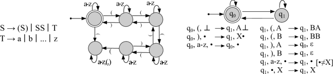
Figure 1: (Left) The context-free grammar for the language balanced parentheses (BP). (Center) A DFA that recognizes BP up to depth 4. (Right) A deterministic pushdown automaton (DPDA) that recognizes BP for all depths. The symbol $\bullet$ is a wildcard and stands for all possible tokens. The DPDA extrapolates to all sequences of BP, the DFA recognizes only those up to nesting depth 4.

We propose state-regularized RNNs as a possible step towards addressing both of the aforementioned problems. State-regularized RNNs (sr-RNNs) are a class of recurrent networks that utilize a stochastic state transition mechanism between cell applications. The stochastic mechanism models a probabilistic state dynamics that lets the sr-RNNs transition between a finite number of learnable states. The parameters of the stochastic mechanism are trained jointly with the parameters of the base RNNs.

sr-RNNs have several advantages over standard RNNs. First, instead of having to apply post-training DFA extraction, sr-RNNs determine their (probabilistic and deterministic) state transition behavior more directly. We propose a method that extracts DFAs truly representing the state transition behavior of the underlying RNNs. Second, we hypothesize that the frequently-observed poor extrapolation behavior of RNNs is caused by memorization with hidden states. It is known that RNNs – even those with cell states or external memory – tend to memorize mainly with their hidden states and in an unstructured manner (Strobelt et al., 2016; Hao et al., 2018). We show that the state-regularization mechanism shifts representational power to memory components such as the cell state, resulting in improved extrapolation performance.

We support our hypotheses through experiments both on synthetic and real-world datasets. We explore the improvement of the extrapolation capabilities of sr-RNNs and closely investigate their memorization behavior. For state-regularized LSTMs, for instance, we observe that memorization can be shifted entirely from the hidden state to the cell state. For text and visual data, state-regularization provides more intuitive interpretations of the RNNs’ behavior.

2 Background

We provide some background on deterministic finite automata (DFAs) and deterministic pushdown automata (DPDAs) for two reasons. First, one contribution of our work is a method for extracting DFAs from RNNs. Second, the state regularization we propose is intended to make RNNs behave more like DPDAs and less like DFAs by limiting their ability to memorize with hidden states.

A DFA is a state machine that accepts or rejects sequences of tokens and produces one unique computation path for each input. Let $\Sigma^{*}$ be the language over the alphabet $\Sigma$ and let $\epsilon$ be the empty sequence. A DFA over an alphabet (set of tokens) $\Sigma$ is a 5-tuple $(\mathcal{Q},\Sigma,\delta,q_{0},F)$ consisting of finite set of states $\mathcal{Q}$; a finite set of input tokens $\Sigma$ called the input alphabet; a transition functions $\delta:\mathcal{Q}\times\Sigma\rightarrow\mathcal{Q}$; a start state $q_{0}$; and a set of accept states $F\subseteq\mathcal{Q}$. A sequence $w$ is accepted by the DFA if the application of the transition function, starting with $q_{0}$, leads to an accepting state. Figure 1(center) depicts a DFA for the language of balanced parentheses (BP) up to depth 4. A language is regular if and only if it is accepted by a DFA.

A pushdown automata (PDA) is defined as a 7-tuple $(\mathcal{Q},\Sigma,\Gamma,\delta,q_{0},\perp,F)$ consisting of a finite set of states $\mathcal{Q}$; a finite set of input tokens $\Sigma$ called the input alphabet; a finite set of tokens $\Gamma$ called the stack alphabet; a transition function $\delta\subseteq\mathcal{Q}\times(\Sigma\cup\epsilon)\times\Gamma\rightarrow\mathcal{Q}\times\Gamma^{*}$; a start state $q_{0}$; the initial stack symbol $\perp$; and a set of accepting states $F\subseteq\mathcal{Q}$. Computations of the PDA are applications of the transition relations. The computation starts in $q_{0}$ with the initial stack symbol $\perp$ on the stack and sequence $w$ as input. The pushdown automaton accepts $w$ if after reading $w$ the automaton reaches an accepting state. Figure 1(right) depicts a deterministic PDA for the language BP.

3 State-Regularized Recurrent Networks

The standard recurrence of an RNN is $\mathbf{h}_{t}=f\left(\mathbf{h}_{t-1},\mathbf{c}_{t-1},\mathbf{x}_{t}\right)$ where $\mathbf{h}_{t}$ is the hidden state vector at time $t$, $\mathbf{c}_{t}$ is the cell state at time $t$, and $\mathbf{x}_{t}$ is the input symbol at time $t$. We refer to RNNs whose unrolled cells are only connected through the hidden output states $\mathbf{h}$ and no additional vectors such as the cell state, as memory-less RNNs. For instance, the family of GRUs (Chung et al., 2014) does not have cell states and, therefore, is memory-less. LSTMs (Hochreiter & Schmidhuber, 1997), on the other hand, are not memory-less due to their cell state.

A cell of a state-regularized RNN (sr-RNN) consist of two components. The first component, which we refer to as the recurrent component, applies the function of a standard RNN cell

$$\mathbf{u}_{t}=f\left(\mathbf{h}_{t-1},\mathbf{c}_{t-1},\mathbf{x}_{t}\right).$$ (1)

For the sake of completeness, we include the cell state $\mathbf{c}$ here, which is absent in memory-less RNNs.

We propose a second component which we refer to as stochastic component. The stochastic component is responsible for modeling the probabilistic state transitions that let the RNN transition implicitly between a finite number of states. Let $d$ be the size of the hidden state vectors of the recurrent cells. Moreover, let $\Delta^{D}:=\{\bm{\lambda}\in\mathbb{R}_{+}^{D}:\parallel\bm{\lambda}\parallel=1\}$ be the $(D-1)$ probability simplex. The stochastic component maintains $k$ learnable centroids $\mathbf{s}_{1}$, …, $\mathbf{s}_{k}$ of size $d$ which we often write as the column vectors of a matrix $\mathbf{S}\in\mathbb{R}^{d\times k}$. The weights of these centroids are global parameters shared among all cells. The stochastic component computes, at each time step $t$, a discrete probability distribution from the output $\mathbf{u}_{t}$ of the recurrent component and the centroids of the stochastic component

$$\bm{\alpha}=g(\mathbf{S},\mathbf{u}_{t})\mbox{ with }\bm{\alpha}\in\Delta^{k}.$$ (2)

Crucially, instances of $g$ should be differentiable to facilitate end-to-end training. Typical instances of the function $g$ are based on the dot-product or the Euclidean distance, normalized into a probability distribution

$$\alpha_{i}= \frac{\exp\left((\mathbf{u}_{t}\cdot\mathbf{s}_{i})/\tau\right)}{\sum_{i=1}^{k}\exp\left((\mathbf{u}_{t}\cdot\mathbf{s}_{i})/\tau\right)}$$ (3)

$$\alpha_{i}= \frac{\exp\left(-\parallel\mathbf{u}_{t}-\mathbf{s}_{i}\parallel/\tau\right)}{\sum_{i=1}^{k}\exp\left(-\parallel\mathbf{u}_{t}-\mathbf{s}_{i}\parallel/\tau\right)}$$ (4)

Here, $\tau$ is a temperature parameter that can be used to anneal the probabilistic state transition behavior. The lower $\tau$ the more $\bm{\alpha}$ resembles the one-hot encoding of a centroid. The higher $\tau$ the more uniform is $\bm{\alpha}$. Equation 3 is reminiscent of the equations of attentive mechanisms (Bahdanau et al., 2015; Vaswani et al., 2017). Instead of attending to the hidden states, however, sr-RNNs attend to the $k$ centroids to compute transition probabilities. Each $\alpha_{i}$ is the probability of the RNN to transition to centroid (state) $i$ given the vector $\mathbf{u}_{t}$ for which we write $p_{\mathbf{u}_{t}}(i)=\alpha_{i}$.

The state transition dynamics of an sr-RNN is that of a probabilistic finite state machine. At each time step, when being in state $\mathbf{h}_{t-1}$ and reading input symbol $\mathbf{x}_{t}$, the probability for transitioning to state $\mathbf{s}_{i}$ is $\alpha_{i}$. Hence, in its second phase the stochastic component computes the hidden state $\mathbf{h}_{t}$ at time step $t$ from the distribution $\bm{\alpha}$ and the matrix $\mathbf{S}$ with a (possibly stochastic) mapping $h:\Delta^{k}\times\mathbb{R}^{d\times k}\rightarrow\mathbb{R}^{d}$. Hence, $\mathbf{h}_{t}=h(\bm{\alpha},\mathbf{S})$. An instance of $h$ is to

$$\mbox{sample }j\sim p_{\mathbf{u}_{t}}\mbox{ and set }\mathbf{h}_{t}=\mathbf{s}_{j}.$$ (5)

This renders the sr-RNN not end-to-end differentiable, however, and one has to use EM or reinforcement learning strategies which are often less stable and less efficient. A possible alternative is to set the hidden state $\mathbf{h}_{t}$ to be the probabilistic mixture of the centroids

$$\mathbf{h}_{t}=\sum_{i=1}^{k}\alpha_{i}\mathbf{s}_{i}.$$ (6)

Every internal state $\mathbf{h}$ of the sr-RNN, therefore, is computed as a weighted sum $\mathbf{h}=\alpha_{1}\mathbf{s}_{1}+...+\alpha_{k}\mathbf{s}_{k}$ of the centroids $\mathbf{s}_{1},...,\mathbf{s}_{k}$ with $\bm{\alpha}\in\Delta^{k}$. Here, $h$ is a smoothed variant of the function that computes a hard assignment to one of the centroids. One can show that for $\tau\rightarrow 0$ the state dynamics based on equations (4) and (5) are identical and correspond to those of a DFA. Figure 2 depicts two variants of the proposed sr-RNNs.

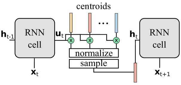
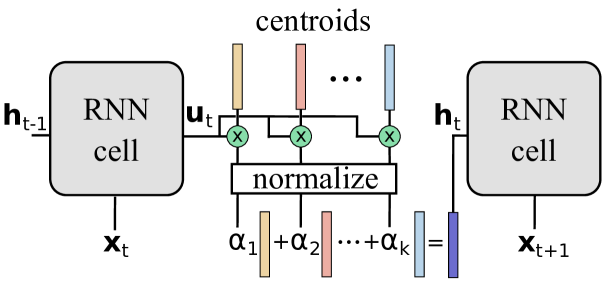
Figure 2: Two possible instances of an sr-RNN corresponding to equations 3&5 and  3&6.

Additional instances of $h$ are conceivable. For instance, one could, for every input sequence and the given current parameters of the sr-RNN, compute the most probable state sequence and then backpropagate based on a structured loss. Since finding these most probable sequences is possible with Viterbi type algorithms, one can apply a form of differentiable dynamic programming (Mensch & Blondel, 2018). The probabilistic state transitions of sr-RNNs open up new possibilities for applying more complex differentiable functions. We leave these considerations to future work. The probabilistic state transition mechanism is also applicable when RNNs have more than one hidden layer. In RNNs with $l>1$ hidden layers, every such layer can maintain its own centroids and stochastic component. In this case, a global state of the sr-RNN is an $l$-tuple, with the $l{\mbox{th}}$ argument of the tuple corresponding to the centroids of the $l{\mbox{th}}$ layer.

Even though we have augmented the original RNN with additional learnable parameter vectors, we are actually constraining the sr-RNN to output hidden state vectors that are similar to the centroids. For lower temperatures and smaller values for $k$, the ability of the sr-RNN to memorize with its hidden states is increasingly impoverished. We argue that this behavior is beneficial for three reasons. First, it makes the extraction of interpretable DFAs from memory-less sr-RNNs straight-forward. Instead of applying post-training DFA extraction as in previous work, we extract the true underlying DFA directly from the sr-RNN. Second, we hypothesize that overfitting in the context of RNNs is often caused by memorization via hidden states. Indeed, we show that regularizing the state space pushes representational power to memory components such as the cell state of an LSTM, resulting in improved extrapolation behavior. Third, the values of hidden states tend to increase in magnitude with the length of the input sequence, a behavior that has been termed drifting (Zeng et al., 1993). The proposed state regularization stabilizes the hidden states for longer sequences.

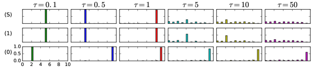
(a)

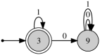
(b)

Figure 3: (Left) State transition probabilities for the sr-GRU learned from the data for the Tomita 1 grammar, for temperatures $\tau$ and input sequence $\mathtt{[10]}$. $\mathtt{S}$ is the start token. Centroids are listed on x-axis, probabilities on y-axis. Up to temperature $\tau=1$ the behavior of the trained sr-GRUs is almost identical to that of a DFA. Despite the availability of $k=10$ centroids, the trained sr-GRUs use the minimal set of states for $\tau\leq 1$. (Right) The extracted DFA for Tomita grammar 1 and temperature $\tau=0.5$.

First, let us explore some of the theoretical properties of the proposed mechanism. We show that the addition of the stochastic component, when capturing the complete information flow between cells as, for instance, in the case of GRUs, makes the resulting RNN’s state transition behavior identical to that of a probabilistic finite state machine.

Theorem 3.1.

The state transition behavior of a memory-less sr-RNN using equation 5 is identical to that of a probabilistic finite automaton.

Theorem 3.2.

For $\tau\rightarrow 0$ the state transition behavior of a memory-less sr-RNN (using equations 5 or 6) is equivalent to that of a deterministic finite automaton.

We can show that the lower the temperature the more memory-less RNNs operate like DFAs. The proofs of the theorems are part of the Supplementary Material.

3.1 Learning DFAs with State-Regularized RNNs

Extracting DFAs from RNNs is motivated by applications where a thorough understanding of learned neural models is required before deployment. sr-RNNs maintain a set of learnable states and compute and explicitly follow state transition probabilities. It is possible, therefore, to extract finite-state transition functions that truly model the underlying state dynamics of the sr-RNN. The centroids do not have to be extracted from a clustering of a number of observed hidden states but can be read off of the trained model. This renders the extraction also more efficient. We adapt previous work (Schellhammer et al., 1998; Wang et al., 2018b) to construct the transition function of a sr-RNN. We begin with the start token of an input sequence, compute the transition probabilities $\bm{\alpha}$, and move the sr-RNN to the highest probability state. We continue this process until we have seen the last input token. By doing this, we get a count of transitions from every state $\mathbf{s}_{i}$ and input token $a\in\Sigma$ to the following states (including selfloops). After obtaining the transition counts, we keep only the most frequent transitions and discard all other transitions. Due to space constraints, the pseudo-code of the extraction algorithm is listed in the Supplementary Material. As a corollary of Theorem 3.2 we have that, for $\tau\rightarrow 0$, the extracted transition function is identical to the transition function of the DFA learned by the sr-RNN. Figure 3 shows that for a wide range of temperatures (including the standard softmax temperature $\tau=1$) the transition behavior of a sr-GRU is identical to that of a DFA, a behavior we can show to be common when sr-RNNs are trained on regular languages.

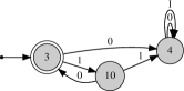
(a)

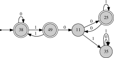
(b)

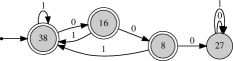
(c)

Figure 4: Extracted DFAs of the Tomita grammars 2-4. The state numbers correspond to the index of the learned sr-GRU centroids.

3.2 Learning Nonregular Languages with State-Regularized LSTMs

Dataset	Large Dataset			Small Dataset
Models	LSTM	sr-LSTM	sr-LSTM-p	LSTM	sr-LSTM	sr-LSTM-p
$d\in{[}1,10{]}$, $l\leq 100$	0.005	0.038	0.000	0.068	0.037	0.017
$d\in{[}10,20{]}$, $l\leq 100$	0.334	0.255	0.001	0.472	0.347	0.189
$d\in{[}10,20{]}$, $l\leq 200$	0.341	0.313	0.003	0.479	0.352	0.196
$d=5$, $l\leq 200$	0.002	0.044	0.000	0.042	0.028	0.015
$d=10$, $l\leq 200$	0.207	0.227	0.004	0.409	0.279	0.138
$d=20$, $l\leq 1000$	0.543	0.540	0.020	0.519	0.508	0.380

Table 1: Error rates for the balanced parentheses (BP) test sets ($d$=depth, $l$=length, $k$=5 centroids, the training depth $\leq 5$).

For more complex languages such as context-free languages, RNNs that behave like DFAs generalize poorly to longer sequences. The DPDA shown in Figure 1, for instance, correctly recognizes the language of BP while the DFA only recognizes it up to nesting depth 4. We want to encourage RNNs with memory to behavor more like DPDAs and less like DFAs. The transition function $\delta$ of a DPDA takes (a) the current state, (b) the current top stack symbol, and (c) the current input symbol and maps these inputs to (1) a new state and (2) a replacement of the top stack symbol (see section 2). Hence, to allow an sr-RNN such as the sr-LSTM to operate in a manner similar to a DPDA we need to give the RNNs access to these three inputs when deciding what to forget from and what to add to memory. Precisely this is accomplished for LSTMs with peephole connections (Gers & Schmidhuber, 2000). The following additions to the functions defining the forget, input, and output gates include the cell state into the LSTM’s memory update decisions

$${\color[rgb]{0.5,0.5,0.5}\mathbf{f}_{t}} {\color[rgb]{0.5,0.5,0.5}=} \ {\color[rgb]{0.5,0.5,0.5}\sigma\big{(}\mathbf{W}^{f}\mathbf{x}_{t}} {\color[rgb]{0.5,0.5,0.5}+} \ {\color[rgb]{0.5,0.5,0.5}\mathbf{R}^{f}\mathbf{h}_{t-1}} + \ {\color[rgb]{0.0,0.0,0.0}\mathbf{p}^{f}\odot\mathbf{c}_{t-1}} {\color[rgb]{0.5,0.5,0.5}+} {\color[rgb]{0.5,0.5,0.5}\mathbf{b}^{f}} {\color[rgb]{0.5,0.5,0.5}\big{)}}$$ (7)

$${\color[rgb]{0.5,0.5,0.5}\mathbf{i}_{t}} {\color[rgb]{0.5,0.5,0.5}=} \ {\color[rgb]{0.5,0.5,0.5}\sigma\big{(}\mathbf{W}^{i}\mathbf{x}_{t}} {\color[rgb]{0.5,0.5,0.5}+} \ {\color[rgb]{0.5,0.5,0.5}\mathbf{R}^{i}\mathbf{h}_{t-1}} + \ {\color[rgb]{0.0,0.0,0.0}\mathbf{p}^{i}\odot\mathbf{c}_{t-1}} {\color[rgb]{0.5,0.5,0.5}+} {\color[rgb]{0.5,0.5,0.5}\mathbf{b}^{i}} {\color[rgb]{0.5,0.5,0.5}\big{)}}$$ (8)

$${\color[rgb]{0.5,0.5,0.5}\mathbf{o}_{t}} {\color[rgb]{0.5,0.5,0.5}=} \ {\color[rgb]{0.5,0.5,0.5}\sigma\big{(}\mathbf{W}^{o}\mathbf{x}_{t}} {\color[rgb]{0.5,0.5,0.5}+} \ {\color[rgb]{0.5,0.5,0.5}\mathbf{R}^{o}\mathbf{h}_{t-1}} + \ {\color[rgb]{0.0,0.0,0.0}\mathbf{p}^{o}\odot\mathbf{c}_{t}} {\color[rgb]{0.5,0.5,0.5}+} {\color[rgb]{0.5,0.5,0.5}\mathbf{b}^{o}} {\color[rgb]{0.5,0.5,0.5}\big{)}}$$ (9)

Here, $\mathbf{h}_{t-1}$ is the output of the previous cell’s stochastic component; $\mathbf{W}$s and $\mathbf{R}$s are the matrices of the original LSTM; the $\mathbf{p}$s are the parameters of the peephole connections; and $\odot$ is the elementwise multiplication. We show empirically that the resulting sr-LSTM-p operates like a DPDA, incorporating the current cell state when making decisions about changes to the next cell state.

3.3 Practical Considerations

Implementing sr-RNNs only requires extending existing RNN cells with a stochastic component. We have found the use of start and end tokens to be beneficial. The start token is used to transition the sr-RNN to a centroid representing the start state which then does not have to be fixed a priori. The end token is used to perform one more cell application but without applying the stochastic component before a classification layer. The end token lets the sr-RNN consider both the cell state and the hidden state to make the accept/reject decision. We find that a temperature of $\tau=1$ (standard softmax) and an initialization of the centroids with values sampled uniformly from $[-0.5,0.5]$ work well across different datasets.

Number of centroids	$k=2$	$k=5$	$k=10$	$k=50$
$d\in{[}1,10{]}$, $l\leq 100$	0.019	0.017	0.021	0.034
$d\in{[}10,20{]}$, $l\leq 100$	0.096	0.189	0.205	0.192
$d\in{[}10,20{]}$, $l\leq 200$	0.097	0.196	0.213	0.191
$d=5$, $l\leq 200$	0.014	0.015	0.012	0.047
$d=10$, $l\leq 200$	0.038	0.138	0.154	0.128
$d=20$, $l\leq 1000$	0.399	0.380	0.432	0.410

Figure 5: Error rates of the sr-LSTM-p on the small BP test data for various numbers of centroids $k$ ($d$=depth, $l$=length).

[5cm]

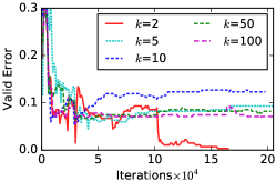
Figure 6: sr-LSTM-p error curves on the small BP validation data.

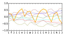
(a) $\mathbf{h}_{t}$ of the LSTM

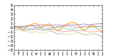
(b) $\mathbf{c}_{t}$ of the LSTM

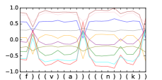
(c) $\mathbf{h}_{t}$ of the sr-LSTM-p

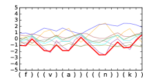
(d) $\mathbf{c}_{t}$ of the sr-LSTM-p

Figure 7: Visualization of hidden state $\mathbf{h}_{t}$ and cell state $\mathbf{c}_{t}$ of the LSTM and the sr-LSTM-p for a specific input sequence from BP. Each color corresponds to one of 10 hidden units. The LSTM memorizes the number of open parentheses both in the hidden and to a lesser extent in the cell state (bold yellow lines). The memorization is not accomplished with saturated gate outputs and a drift is observable for both vectors. The sr-LSTM-p maintains two distinct hidden states (accept and reject) and does not visibly memorize counts through its hidden states. The cell state is used to cleanly memorize the number of open parentheses (bold red line) with saturated gate outputs ($\pm 1$). For sr-LSTM-p, a state vector drift is not observable; solutions with less drift generalize better (Gers & Schmidhuber, 2001).

4 Experiments

We conduct three types of experiments to investigate our hypotheses. First, we apply a simple algorithm for extracting DFAs and assess to what extent the true DFAs can be recovered from input data. Second, we compare the behavior of LSTMs and state-regularized LSTM on nonregular languages such as the languages of balanced parentheses and palindromes. Third, we investigate the performance of state-regularized LSTMs on non-synthetic datasets.

Unless otherwise indicated we always (a) use single-layer RNNs, (b) learn an embedding for input tokens before feeding it to the RNNs, (c) apply RMSprop with a learning rate of $0.01$ and momentum of $0.9$; (d) do not use dropout (Srivastava et al., 2014) or batch normalization (Cooijmans et al., 2017) of any kind; and (e) use state-regularized RNNs based on equations 3&6 with a temperature of $\tau=1$ (standard softmax). We include more experimental results and the code in the Supplementary Material.

4.1 Regular Languages and DFA Extraction

We evaluate the DFA extraction algorithm for sr-RNNs on RNNs trained on the Tomita grammars (Tomita, 1982) which have been used as benchmarks in previous work (Wang et al., 2018b; Weiss et al., 2018b). We use available code (Weiss et al., 2018b) to generate training and test data for the regular languages. We first trained a single-layer GRU with $100$ units on the data. We use GRUs since they are memory-less and, hence, Theorem 3.2 applies. Whenever the GRU converged within 1 hour to a training accuracy of $100\%$, we also trained a sr-GRU based on equations 3&6 with $k=50$ and $\tau=1$. This was the case for the grammars 1-4 and 7. The difference in time to convergence between the vanilla GRU and the sr-GRU was negligible. We applied the transition function extraction outlined in section 3.1. In all cases, we could recover the minimal and correct DFA corresponding to the grammars. Figure 4 depicts the DFAs for grammars 2-4 extracted by our approach. Remarkably, even though we provide more centroids (possible states; here $k=50$) the sr-GRU only utilizes the required minimal number of states for each of the grammars. Figure 3 visualizes the transition probabilities for different temperatures and $k=10$ for grammar 1. The numbers on the states correspond directly to the centroid numbers of the learned sr-GRU. One can observe that the probabilities are spiky, causing the sr-GRU to behave like a DFA for $\tau\leq 1$.

4.2 Nonregular Languages

We conducted experiments on nonregular languages where external memorization is required. We wanted to investigate whether our hypothesis that sr-LSTM behave more like DPDAs and, therefore, extrapolate to longer sequences, is correct. To that end, we used the context-free language “balanced parentheses” (BP; see Figure 1(left)) over the alphabet $\Sigma=\{a,...,z,(,)\}$, used in previous work (Weiss et al., 2018b). We created two datasets for BP. A large one with 22,286 training sequences (positive: 13,025; negative: 9,261) and 6,704 validation sequences (positive: 3,582; negative: 3,122). The small dataset consists of 1,008 training sequences (positive: 601; negative: 407), and 268 validation sequences (positive: 142; negative: 126). The training sequences have nesting depths $d\in[1,5]$ and the validation sequences $d\in[6,10]$. We trained the LSTM and the sr-RNNs using curriculum learning as in previous work (Zaremba & Sutskever, 2014; Weiss et al., 2018b) and using the validation error as stopping criterion. We then applied the trained models to unseen sequences. Table 1 lists the results on 1,000 test sequences each with the respective depths and lengths. The results show that both sr-LSTM and sr-LSTM-ps extrapolate better to longer sequences and sequences with deeper nesting. Moreover, the sr-LSTM-p performs almost perfectly on the large data indicating that peephole connections are indeed beneficial.

To explore the effect of the hyperparameter $k$, that is, the number of centroids of the sr-RNNs, we ran experiments on the small BP dataset varying $k$ and keeping everything else the same. Table 6 lists the error rates and Figure 6 the error curves on the validation data for the sr-LSTM-p and different values of $k$. While two centroids ($k=2$) result in the best error rates for most sequence types, the differences are not very pronounced. This indicates that the sr-LSTM-p is robust to changes in the hyperparameter $k$. A close inspection of the transition probabilities reveals that the sr-LSTM-p mostly utilizes two states, independent of the value of $k$. These two states are used as accept and reject states. These results show that sr-RNNs generalize tend to utilize a minimal set states similar to DPDAs.

A major hypothesis of ours is that the state-regularization encourages RNNs to operate more like DPDAs. To explore this hypothesis, we trained an sr-LSTM-p with $10$ units on the BP data and visualized both the hidden state $\mathbf{h}_{t}$ and the cell state $\mathbf{c}_{t}$ for various input sequences. Similar state visualizations have been used in previous work (Strobelt et al., 2016; Weiss et al., 2018a). Figure 7 plots the hidden and cell states for a specific input, where each color corresponds to a dimension in the respective state vectors. As hypothesized, the LSTM relies primarily on its hidden states for memorization. The sr-LSTM-p, on the other hand, does not use its hidden states for memorization. Instead it utilizes two main states (accept and reject) and memorizes the nesting depth cleanly in the cell state. The visualization also shows a drifting behavior for the LSTM, in line with observations made for first-generation RNNs (Zeng et al., 1993). Drifting is not observable for the sr-LSTM-p.

Max Length	100	200	500
LSTM	31.2	42.0	47.7
LSTM-p	28.4	36.2	41.5
sr-LSTM	28.0	36.0	44.6
sr-LSTM-p	10.5	16.7	29.8

Figure 8: Error rates in $\%$ on sequences of varying lengths from the Palindrome test set.

Model	LSTM		sr-LSTM		LSTM-p		sr-LSTM-p
Length	$100$	$200$	$100$	$200$	$100$	$200$	$100$	$200$
train error	29.23	32.77	27.17	31.72	25.50	29.05	23.30	24.67
test error	29.96	33.19	28.82	32.88	28.02	30.12	26.04	26.21
time (epoch)	400.29s		429.15s		410.29s		466.10s

Figure 9: Error rates (on training and test splits of the IMDB data) in $\%$ and averaged training time in seconds when training only on truncated sequences of length $10$.

Methods	Error
use additional unlabeled data
Full+unlabelled+BoW (Maas et al.)	11.1
LM-LSTM+unlabelled (Dai & Le)	7.6
SA-LSTM+unlabelled (Dai & Le)	7.2
do not use additional unlabeled data
seq2-bown-CNN (Johnson & Zhang)	14.7
WRRBM+BoW(bnc) (Dahl et al.)	10.8
JumpLSTM (Yu et al.)	10.6
LSTM	10.1
LSTM-p	10.3
sr-LSTM ($k=10$)	9.4
sr-LSTM-p ($k=10$)	9.2
sr-LSTM-p ($k=50$)	9.8

Figure 10: Test error rates (%) on IMDB.

Figure 11: Test accuracy on pixel-by-pixel MNIST (%)

Methods	Accuracy
IRNN (Le et al.)	97.0
URNN (Arjovsky et al.)	95.1
Full URNN (Wisdom et al.)	97.5
sTANH-RNN  (Zhang et al.)	98.1
RWA (Ostmeyer & Cowell)	98.1
Skip LSTM (Campos et al.)	97.3
r-LSTM Full BP (Trinh et al.)	98.4
BN-LSTM (Cooijmans et al.)	99.0
Dilated GRU (Chang et al.)	99.2
LSTM	97.7
LSTM-p	98.5
sr-LSTM $(k=100)$	98.6
sr-LSTM-p $(k=100)$	99.2
sr-LSTM-p $(k=50)$	98.6

Figure 12: Test accuracy (%) on sequential MNIST.

We also performed experiments for the nonregular language $ww^{-1}$ (Palindromes) (Schmidhuber et al., 2002) over the alphabet $\Sigma=\{a,...,z\}$. We follow the same experiment setup as for BP and include the details in the Supplementary Material. The results of Table 9 add evidence for the improved generalization and memorization behavior of state-regularized LSTMs over vanilla LSTMs (with peepholes). Additional experimental results on the Copying Memory task are provided in the Supplementary Material.

4.3 Sentiment Analysis and Pixel-by-Pixel MNIST

We evaluated state-regularized LSTMs on the IMDB review dataset (Maas et al., 2011). It consists of 100k movie reviews (25k training, 25k test, and 50k unlabeled). We used only the labeled training and test reviews. Each review is labeled as positive or negative. To investigate the models’ extrapolation capabilities, we trained all models on truncated sequences of up to length $10$ but tested on longer sequences (length 100 and 200). The results listed in Table 9 show the improvement in extrapolation performance of the sr-LSTM-p. The table also lists the training time per epoch, indicating that the overhead compared to the standard LSTM (or with peepholes LSTM-p) is modest. Table 12 lists the results when training without truncating sequences. The sr-LSTM-p is competitive with state of the art methods that also do not use the unlabeled data.

We also explored the impact of state-regularization on pixel-by-pixel MNIST (LeCun et al., 1998; Le et al., 2015). Here, the 784 pixels of MNIST images are fed to RNNs one by one for classification. This requires the modeling of long-term dependencies. Table 12 shows the results on the normal and permuted versions of pixel-by-pixel MNIST. The classification function has the final hidden and cell state as input. Our (state-regularized) LSTMs do not use dropout, batch normalization, sophisticated weight-initialization, and are based on a simple single-layer LSTM. We can observe that sr-LSTM-ps achieve competitive results, outperforming the vanilla LSTM and LSTM-P. The experiments on the Language Modeling is in the Supplementary Material.

cent.	words with top-$4$ highest transition probabilities
1	but (0.97) hadn (0.905) college (0.87) even (0.853)
2	not (0.997) or (0.997) italian (0.995) never (0.993)
3	loved (0.998) definitely (0.996) 8 (0.993) realistic (0.992)
4	no (1.0) worst (1.0) terrible (1.0) poorly (1.0)

Figure 13: The learned centroids and their prototypical words with the top-4 highest transition probabilities. This interprets the sr-LSTM-p model with centroids. The $3^{rd}$ ($4^{th}$) centroid is “positive” (“negative”).

[7.5cm]

Figure 14: The prototypes of generated by learned sr-LSTM-p ($k$$=$$10$) centroids for “3” in MNIST (top) and “T-shirt” in Fashion-MNIST (bottom) (Xiao et al., 2017).

4.4 Interpretability and Explainability

State-regularization provides new ways to interpret the working of RNNs. Since sr-RNNs have a finite set of states, we can use the observed transition probabilities to visualize their behavior. For instance, to generate prototypes for the sr-RNNs we can select, for each state $i$, the input tokens that have the highest average probability leading to state $i$. For the IMDB reviews, these are the top probability words leading to each of the states. For pixel-by-pixel MNIST, these are the top probabilities of each pixel leading to the states. Table 14 lists, for each state (centroid), the word with the top transition probabilities leading to this state. Figure 14 shows the prototypes associated with digits “3” of MNIST and “T-shirt” of Fashion-MNIST. In contrast to previous methods (Berkes & Wiskott, 2006; Nguyen et al., 2016), the prototypes are directly generated with the centroids of the trained sr-RNNs and the input token embeddings and hidden states do not have to be similar. For more evidence of generated interpretations and explanations, we refer to the Supplementary Material.

5 Related Work

RNNs are powerful learning machines. Siegelmann and Sontag (Siegelmann & Sontag, 1992, 1994; Siegelmann, 2012), for instance, proved that a variant of Elman-RNNs (Elman, 1990) can simulate a Turing machine. Recent work considers the more practical situation where RNNs have finite precision and linear computation time in their input length (Weiss et al., 2018a).

Extracting DFAs from RNNs goes back to work on first-generation RNNs in the 1990s(Giles et al., 1991; Zeng et al., 1993). These methods perform a clustering of hidden states after the RNNs are trained (Wang et al., 2018a; Frasconi & Bengio, 1994; Giles et al., 1991). Recent work introduced more sophisticated learning approaches to extract DFAs from LSTMs and GRUs (Weiss et al., 2018b). The latter methods tend to be more successful in finding DFAs behaving similar to the RNN. In contrast to all existing methods, sr-RNNs learn an explicit set of states which facilitates the extraction of DFAs from memory-less sr-RNNs exactly modeling their state transition dynamics. A different line of work attempt to learn more interpretable RNNs (Foerster et al., 2017), or rule-based classifiers from RNNs (Murdoch & Szlam, 2017).

There is a large body of work on regularization techniques for RNNs. Most of these adapt regularization approaches developed for feed-forward networks to the recurrent setting. Representative instances are dropout regularization (Zaremba et al., 2014), variational dropout (Gal & Ghahramani, 2016), weight-dropped LSTMs (Merity et al., 2018), and noise injection (Dieng et al., 2018). Two approaches that can improve convergence and generalization capabilities are batch normalization (Cooijmans et al., 2017) and weight initialization strategies (Le et al., 2015) for RNNs. The work most similar to sr-RNNs are self-clustering RNNs (Zeng et al., 1993). These RNNs learn discretized states, that is, binary valued hidden state vectors, and show that these networks generalize better to longer input sequences. Contrary to self-clustering RNNs, we propose an end-to-end differentiable probabilistic state transition mechanism between cell applications.

Stochastic RNNs are a class of generative recurrent models for sequence data (Bayer & Osendorfer, 2014; Fraccaro et al., 2016; Goyal et al., 2017). They model uncertainty in the hidden states of an RNN by introducing latent variables. Contrary to sr-RNNs, stochastic RNNs do not model probabilistic state transition dynamics. Hence, they do not address the problem of overfitting through hidden state memorization and improvements to DFA extraction.

There are proposals for extending RNNs with various types of external memory. Representative examples are the neural Turing machine (Graves et al., 2014), improvements thereof (Graves et al., 2016), memory network (Weston et al., 2015), associative LSTM (Danihelka et al., 2016), and RNNs augmented with neural stacks, queues, and deques (Grefenstette et al., 2015). Contrary to these proposals, we do not augment RNNs with differentiable data structures but regularize RNNs to make better use of existing memory components such as the cell state. We hope, however, that differentiable neural computers could benefit from state-regularization.

6 Discussion and Conclusion

State-regularization provides new mechanisms for understanding the workings of RNNs. Inspired by recent DFA extraction work (Weiss et al., 2018b), our work simplifies the extraction approach by directly learning a finite set of states and an interpretable state transition dynamics. Even on realistic tasks such as sentiment analysis, exploring the learned centroids and the transition behavior of sr-RNNs makes for more interpretable RNN models whithout sacrificing accuracy: a single-layer sr-RNNs is competitive with state-of-the-art methods. The purpose of our work is not to surpass all existing state of the art methods but to gain a deeper understanding of the dynamics of RNNs.

State-regularized RNNs operate more like automata with external memory and less like DFAs. This results in a markedly improved extrapolation behavior on several datasets. We do not claim, however, that sr-RNNs are a panacea for all problems associated with RNNs. For instance, we could not observe an improved convergence of sr-RNNs. Sometimes sr-RNNs converged faster, sometimes vanilla RNNs. While we have mentioned that the computational overhead of sr-RNNs is modest, it still exists, and this might exacerbate the problem that RNNs often take a long to be trained and tuned. We plan to investigate variants of state regularization and the ways in which it could improve differentiable computers with RNN controllers.

Appendix A Proofs of Theorems 3.1 and 3.2

A.1 Theorem 3.1

The state transition behavior of a memory-less sr-RNN using equation 5 is identical to that of a probabilistic finite automaton.

$$\alpha_{i}= \frac{\exp\left(b_{i}/\tau\right)}{\exp(\left(b_{M}-\epsilon_{1})/\tau\right)+...+\exp\left(b_{M}/\tau\right)+...+\exp(\left(b_{M}-\epsilon_{k})/\tau\right)}$$ (10)

$$=\frac{\exp\left(b_{i}/\tau\right)}{\exp(b_{M}/\tau)\exp(\epsilon_{1}/\tau)^{-1}+...+\exp(b_{M}/\tau)+...+\exp(b_{M}/\tau)\exp(\epsilon_{k}/\tau)^{-1}}$$ (11)

$$=\frac{\exp\left(b_{i}/\tau\right)}{\exp(b_{M}/\tau)\left[\exp(\epsilon_{1}/\tau)^{-1}+...+1+...+\exp(\epsilon_{k}/\tau)^{-1}\right]}.$$ (12)

Proof.

The state transition function $\delta$ of a probabilistic finite state machine is identical to that of a finite deterministic automaton (see section 2) with the exception that it returns a probability distribution over states. For every state $q$ and every input token $a$ the transition mapping $\delta$ returns a probability distribution $\bm{\alpha}=(\alpha_{1},...,\alpha_{k})$ that assigns a fixed probability to each possible state $q\in\mathcal{Q}$ with $|\mathcal{Q}|=k$. The automaton transitions to the next state according to this distribution. Since by assumption the sr-RNN is using equation 5, we only have to show that the probability distribution over states computed by the stochastic component of a memory-less sr-RNN is identical for every state $q$ and every input token $a$ irrespective of the previous input sequence and corresponding state transition history.

More formally, for every pair of input token sequences $\mathbf{a}_{1}$ and $\mathbf{a}_{2}$ with corresponding pair of resulting state sequences $\mathbf{q}_{1}=(q_{i_{1}},...,q_{i_{n}},q)$ and $\mathbf{q}_{2}=(q_{j_{1}},...,q_{j_{m}},q)$ in the memory-less sr-RNN, we have to prove, for every token $a\in\Sigma$, that $\bm{\alpha}_{1}$ and $\bm{\alpha}_{2}$, the probability distributions over the states returned by the stochastic component for state $q$ and input token $a$, are identical. Now, since the RNN is, by assumption, memory-less, we have for both $\mathbf{a}_{1},\mathbf{q}_{1}$ and $\mathbf{a}_{2},\mathbf{q}_{2}$ that the only inputs to the RNN cell are exactly the centroid $\mathbf{s}_{q}$ corresponding to state $q$ and the vector representation of token $a$. Hence, under the assumption that the parameter weights of the RNN are the same for both state sequences $\mathbf{q}_{1}$ and $\mathbf{q}_{2}$, we have that the output $\mathbf{u}$ of the recurrent component (the base RNN cell) is identical for $\mathbf{q}_{1}$ and $\mathbf{q}_{2}$. Finally, since by assumption the centroids $\mathbf{s}_{1},...,\mathbf{s}_{k}$ are fixed, we have that the returned probability distributions $\bm{\alpha}_{1}$ and $\bm{\alpha}_{2}$ are identical. Hence, the memory-less sr-RNN’s transition behavior is identical to that of a probabilistic finite automaton. ∎

Table 2: A summary of dataset and experiment characteristics. The values in parentheses are the number of positive sequences.

Task	Architecture	Units	$k$	Train	Valid	Test
Tomita 1	sr-GRU	100	5, 10, 50	265 (12)	182 (4)	–
Tomita 2	sr-GRU	100	10, 50	257 (6)	180 (2)	–
Tomita 3	sr-GRU	100	50	2141 (1028)	1344 (615)	–
Tomita 4	sr-GRU	100	50	2571 (1335)	2182(1087)	–
Tomita 5	sr-GRU	100	50	1651 (771)	1298(608)	–
Tomita 6	sr-GRU	100	50	2523 (1221)	2222(1098)	–
Tomita 7	sr-GRU	100	50	1561 (745)	680(288)	–
BP (large)	sr-LSTM (-P)	100	5	22286 (13025)	6704 (3582)	1k
BP (small)	sr-LSTM (-P)	100	2,5,10,50,100	1008 (601)	268 (142)	1k
Palindrome	sr-LSTM (-P)	100	5	229984 (115040)	50k(25k)	1k
IMDB (full)	sr-LSTM (-P)	256	2,5,10	25k	–	25k
IMDB (small)	sr-LSTM (-P)	256	2,5,10	25k	–	25k
MNIST (normal)	sr-LSTM (-P)	256	10,50,100	60k	–	10k
MNIST (perm.)	sr-LSTM (-P)	256	10,50,100	60k	–	10k
Fashion-MNIST	sr-LSTM (-P)	256	10	55k	5k	10k
Copying Memory	sr-LSTM (-P)	128, 256	5,10,20	100k	–	10k
Wikipedia	sr-LSTM (-P)	300	1000	22.5M	1.2M	1.2M

Table 3: The lengths ($l$) and depths ($d$) of the sequences in the training, validation, and test sets of the various tasks.

Task	Train $l$ & $d$	Valid $l$ & $d$	Test $l$ & $d$
Tomita 1 -7	$l$ = 0$\sim$13, 16, 19, 22	$l$ = 1, 4,…, 28	–
BP (large)	$d\in[1,5]$	$d\in[6,10]$	$d\in[1,20]$
BP (small)	$d\in[1,5]$	$d\in[6,10]$	$d\in[1,20]$
Palindrome	$l\in[1,25]$	$l\in[26,50]$	$l\in[50,500]$
IMDB (full)	$l\in[11,2820],l_{aver}=285$	–	$l\in[8,2956],l_{aver}=278$
IMDB (small)	$l=10$	–	$l\in[100,200]$
MNIST(normal)	$l=784$	$l=784$	$l=784$
MNIST(perm.)	$l=784$	$l=784$	$l=784$
Fashion-MNIST	$l=784$	$l=784$	$l=784$
Copying Memory	$l=100,500$	–	$l=100,500$
Wikipedia	$l=22.5M$	$l=1.2M$	$l=1.2M$

A.2 Theorem 3.2

For $\tau\rightarrow 0$ the state transition behavior of a memory-less sr-RNN (using equations 5 or 6) is identical to that of a deterministic finite automaton.

Proof.

Let us consider the softmax function with temperature parameter $\tau$

$$\alpha_{i}=\frac{\exp\left(b_{i}/\tau\right)}{\sum_{i=1}^{k}\exp\left(b_{i}/\tau\right)}$$

for $1\leq i\leq k$. sr-RNNs use this softmax function to normalize the scores (from a dot product or Euclidean distance) into a probability distribution. First, we show that for $\tau\rightarrow 0^{+}$, that there is exactly one $M\in\{1,...,k\}$ such that $\alpha_{M}=1$ and $\alpha_{i}=0$ for all $i\in\{1,...,k\}$ with $i\neq M$. Without loss of generality, we assume that there is a $M\in\{1,...,k\}$ such that $b_{M}>b_{i}$ for all $i\in\{1,...,k\},i\neq M$. Hence, we can write for $\epsilon_{1},...,\epsilon_{k}>0$ as shown in equations (10-12).

Now, for $\tau\rightarrow 0$ we have that $\alpha_{M}\rightarrow 1$ and for all other $i\neq M$ we have that $\alpha_{i}\rightarrow 0$. Hence, the probability distribution $\bm{\alpha}$ of the sr-RNN is always the one-hot encoding of a particular centroid.

By an argument analog to the one we have made for Theorem 3.1, we can prove that for every state $q\in\mathcal{Q}$ and every input token $a\in\Sigma$, the probability distribution $\bm{\alpha}$ of the sr-RNN is the same irrespective of the previous input sequences and visited states. Finally, by plugging in the one-hot encoding $\bm{\alpha}$ in both equations 5 and 6, we can conclude that the transition function of a memory-less sr-RNN is identical to that of a DFA, because we always chose exactly one new state. ∎

Appendix B Implementation Details

Unless otherwise indicated we always (a) use single-layer RNNs, (b) learn an embedding for input tokens before feeding it to the RNNs, (c) apply RMSprop with a learning rate of $0.01$ and momentum of $0.9$; (d) do not use dropout or batch normalization of any kind; and (e) use state-regularized RNNs based on equations 3&6 with a temperature of $\tau=1$ (standard softmax). We implemented sr-RNNs with Theano(Theano Development Team, 2016) . The hyper-parameter were tuned to make sure the vanilla RNNs achieves the best performance. For sr-RNNs we tuned the weight initialization values for the centroids and found that sampling uniformly from the interval $[-0.5,0.5]$ works well across different datasets. Table 2 lists some statistics about the datasets and the experimental set-ups. Table 3 shows the length and nesting depth (if applicable) for the sequences in the train, validation, and test datasets.

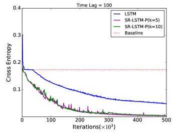
(a)

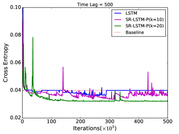
(b)

Figure 15: The results (test cross entropy loss) on copying memory problem for time lags $T=100$ (left) and $T=500$ (right). We used one recurrent layer with 128 hidden units for $T=100$, and 256 hidden units for $T=500$.

Appendix C Experiments on Copying Memory Problem

Besides the introduced balanced paretness, palindrome task, we also conducted experiment on the copying memory problem (Hochreiter & Schmidhuber, 1997). We follow the similar setup as described in (Hochreiter & Schmidhuber, 1997; Arjovsky et al., 2016; Jing et al., 2017). The alphabet $\Sigma$ has 10 characters $\Sigma=\{c_{i}\}_{i=0}^{9}$. The input and output sequences have lengths of $T+2n$, where $T$ is the time lag and $n$ is the length of sequence that need to be memorized and copied. The exemplary input and output are listed as follows.

Input:  $c_{1}$$c_{4}$$c_{2}$$c_{1}$$c_{8}$$c_{4}$$c_{7}$$c_{3}$$c_{5}$$c_{6}$_________$c_{9}$_____

Output: ______________$c_{1}$$c_{4}$$c_{2}$$c_{1}$$c_{8}$$c_{4}$$c_{7}$$c_{3}$$c_{5}$$c_{6}$

We use $n=10$, the first $n$ symbols of input sequence are uniformly sampled from $[c_{1},c_{8}]$, the $c_{0}$ is used as “blank” symbol (as shown as “_” in above examples. The length of “blank” sequence is $T$). The $c_{9}$ is used as an indicator to require algorithms or models to reproduce the first $n$ symbols with exactly same sequential order. The task is to minimize the average categorical cross entropy at each time step. Similar to (Jing et al., 2017), we used 100000 samples for training and 10000 for test. Differently, all RNN models have only one recurrent layer. We used 128 hidden units for $T=100$ and 256 hidden units for $T=500$. The batch size is set to 128. We use RMSprop with a learning rate of $0.001$ and decay of $0.9$. A simple baseline is a memoryless strategy, which has categorical cross entropy $\frac{10\log(8)}{T+20}$.

Figure 15 presents the performance of the proposed method on copying memory problem for $T=100$ and $T=500$. For time log $T=100$, both standard LSTM and sr-LSTM-ps are able to beat baseline. Clearly we can see the faster convergence of sr-LSTM-ps. For $T=500$, LSTM is hard to beat the baseline, while sr-LSTM-ps outperforms baseline in a certain margin. Both figures demonstrate the memorization capability of sr-LSTM-ps over standard LSTM.

Table 4: The perplexity results for the sr-LSTMs and state of the art methods. Here, $\theta_{W+M}$ are the number of model parameters and $\theta_{M}$ the number of model parameters without word representations. $a$ is the attention window size.

Model	$a$	$\theta_{W+M}$	$\theta_{M}$	Dev	Test
RNN	-	47.0M	23.9M	121.7	125.7
LSTM	-	47.0M	23.9M	83.2	85.2
FOFE HORNN(3-rd order)(Soltani & Jiang, 2016)	-	47.0M	23.9M	116.7	120.5
Gated HORNN(3-rd order)(Soltani & Jiang, 2016)	-	47.0M	23.9M	93.9	97.1
RM(+tM-g) (Tran et al., 2016)	15	93.7M	70.6M	78.2	80.1
Attention (Daniluk et al., 2017b)	10	47.0M	23.9M	80.6	82.0
Key-Value (Daniluk et al., 2017b)	10	47.0M	23.9M	77.1	78.2
Key-Value Predict (Daniluk et al., 2017b)	5	47.0M	23.9M	74.2	75.8
4-gram RNN (Daniluk et al., 2017b)	-	47.0M	23.9M	74.8	75.9
LSTM-p	-	47.0M	23.9M	85.8	86.9
sr-LSTM ($k=1000$)	-	47.3M	24.2M	80.9	82.7
sr-LSTM-p ($k=1000$)	-	47.3M	24.2M	80.2	81.3

Appendix D Experiments on Language Modeling

We evaluated the sr-LSTMs on language modeling task with the Wikipedia dataset (Daniluk et al., 2017b). It consists of 7500 English Wikipedia articles. We used the same experimental setup as in previous work (Daniluk et al., 2017b). We used the provided training, validation, and test dataset: 22.5M words in the training set, 1.2M in the validation, and 1.2M words in the test set. We used the 77k most frequent words from the training set as vocabulary. We report the results in Table 4. We use the model with the best perplexity on the on the validation set. Note that we only tuned the number of centroids for sr-LSTM and sr-LSTM-p and used the same hyperparameters that were used for the vanilla LSTMs.

The results show that the perplexity results for the sr-LSTM and sr-LSTM-p outperform those of the vanilla LSTM and LSTM with peephole connection. The difference, however, is modest and we conjecture that the ability to model long-range dependencies is not that important for this type of language modeling tasks. This is an observation that has also been made by previous work (Daniluk et al., 2017b). The perplexity of the sr-LSTMs cannot reach that of state of the art methods. The methods, however, all utilize a mechanism (such as attention) that allows the next-word decision to be based on a number of past hidden states. The sr-LSTMs, in contrast, makes the next-word decision only based on the current hidden state.

Appendix E Tomita Grammars and DFA Extraction

The Tomita grammars are a collection of 7 regular languages over the alphabet {0,1} (Tomita, 1982). Table 5 lists the regular grammars defining the Tomita grammars.

Grammars	Descriptions
1	1∗
2	(10)∗
3	An odd number of consecutive 1s is followed by an even number of consecutive 0s
4	Strings not contain a substring “000”
5	The numbers of 1s and 0s are even
6	The difference of the numbers of 1s and 0s is a multiple of 3
7	0∗1∗0∗1∗

Table 5: The seven Tomita grammars (Tomita, 1982).

We follow previous work (Wang et al., 2018b; Schellhammer et al., 1998) to construct the transition function of the DFA (deterministic finite automata).

[htb]   Computes DFA transition function Input: pre-trained sr-RNN, dataset D, alphabet $\Sigma$, start token $\mathtt{s}$ Output: transition function $\delta$ of the DFA for $i,j\in\{1,...,k\}\mbox{ and all }x\in\Sigma$ do

       $\bm{\mathcal{T}}[(c_{i},x_{t},c_{j})]=0$ # initialize transition counts to zero

end for

$\{p_{i}\}_{i=1}^{k}\leftarrow\textsc{sr-RNN}(\mathtt{s})$    # compute the transition probabilities for the start token
$j=\operatorname*{arg\,max}_{i\in\{1,...,k\}}(p_{i})$    # determine $j$ the centroid with max transition probability
$c_{0}=j$    # set the start centroid $c_{0}$ to $j$
for $\mathbf{x}=(x_{1},x_{2},...,x_{T})\in\textbf{D}$ do

       for $t\in[1,...,T]$ do

             $\{p_{j}\}_{j=1}^{k}\leftarrow\textsc{sr-RNN}(x_{t})$    # compute the transition probabilities for the $t$-th token
$j=\operatorname*{arg\,max}_{i\in\{1,...,k\}}(p_{i})$    # determine $j$ the centroid with max transition probability
$c_{t}=j$    # set $c_{t}$, the centroid in time step $t$, to $j$
$\bm{\mathcal{T}}[(c_{t-1},x_{t},c_{t})]\leftarrow\bm{\mathcal{T}}[(c_{t-1},x_{t},c_{t})]+1$ # increment transition count

       end for

      

end for

for $i\in\{1,...,k\}\mbox{ and }x\in\Sigma$ do

       $\delta(i,x)=\operatorname*{arg\,max}_{j\in\{1,...,k\}}\bm{\mathcal{T}}[(i,x,j)]$    # compute the transition function of the DFA

end for

return $\delta$
 

We follow earlier work (Weiss et al., 2018b) and attempt to train a GRU to reach 100% accuracy for both training and validation data. We first trained a single-layer GRU with $100$ units on the data. We use GRUs since they are memory-less. Whenever the GRU converged within 1 hour to a training accuracy of $100\%$, we also trained a sr-GRU based on equations 3&6 with $k=50$ and $\tau=1$. This was the case for the grammars 1-4 and 7. For grammar 5 and 6, our experiments show that both vanilla GRU and sr-GRU were not able to achieve 100% accuracy. In this case, sr-GRU (97.2% train and 96.8% valid accuracy) could not extract the correct DFA for grammar 5 and 6. The exploration of deeper GRUs and their corresponding sr-GRUs (2 layers as in (Weiss et al., 2018b) for DFA extraction could be interesting future work.

Algorithm E lists the pseudo-code of the algorithm that constructs the transition function of the DFA. Figure 16 shows the extracted DFA for grammar 7. All DFA visualization in the paper are created with GraphViz .

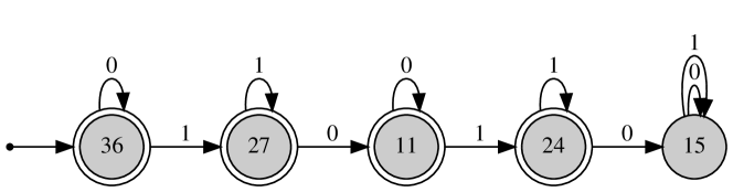
Figure 16: The DFA extracted from the sr-GRU for Tomita grammar 7. The numbers inside the circles correspond to the centroid indices of the sr-GRU. Double circles indicate accept states.

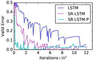
(a)

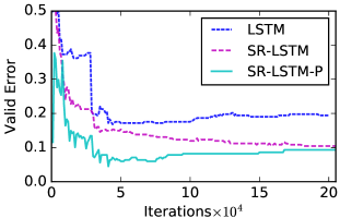
(b)

Figure 17: The error curves on the validation data for the LSTM, sr-LSTM, and sr-LSTM-p ($k=5$)on the large BP dataset (left) and the small BP dataset (right).

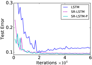
(a)

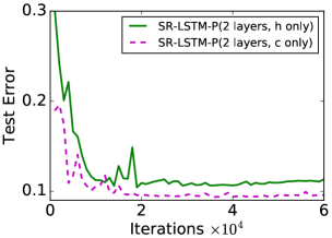
(b)

Figure 18: The error curves on the test data for the LSTM, sr-LSTM, sr-LSTM-p ($k=10$) on the IMDB sentiment analysis dataset. (Left) It shows state-regularized RNNs show better generalization ability. (Right) A 2-layer sr-LSTM-p achieves better error rates when the classification function only looks at the last cell state compared to it only looking at the last hidden state.

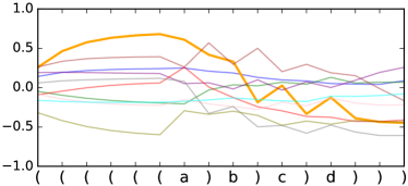
(a) Vector $\mathbf{h}_{t}$ of the LSTM

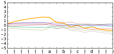
(b) Vector $\mathbf{c}_{t}$ of the LSTM

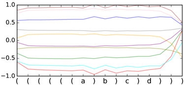
(c) Vector $\mathbf{h}_{t}$ of the sr-LSTM-p

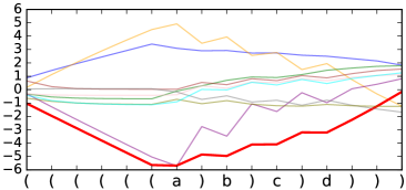
(d) Vector $\mathbf{c}_{t}$ of the sr-LSTM-p

Figure 19: Visualization of hidden state $\mathbf{h}_{t}$ and cell state $\mathbf{c}_{t}$ of the LSTM and the sr-LSTM-p for a specific input sequence from BP. Each color corresponds to one of 10 hidden units. The LSTM memorizes the number of open parentheses both in the hidden and to a lesser extent in the cell state (bold yellow lines). The memorization is not accomplished with saturated gate outputs and a drift is observable for both vectors. The sr-LSTM-p maintains two distinct hidden states (accept and reject) and does not visibly memorize counts through its hidden states. The cell state is used to cleanly memorize the number of open parentheses (bold red line) with saturated gate outputs ($\pm 1$). A state vector drift is not observable (the solutions with less drift to generalize better (Gers & Schmidhuber, 2001)).

Appendix F Training Curves

Figure 17 plots the validation error during training of the LSTM, sr-LSTM, and sr-LSTM-p on the BP (balanced parentheses) datasets. Here, the sr-LSTM and sr-LSTM both have $k=5$ centroids. The state-regularized LSTMs tend to reach better error rates in a shorter amount of iteration.

Figure 18 (left) plots the test error of the LSTM, sr-LSTM, and sr-LSTM-p on the IMDB dataset for sentiment analysis. Here, the sr-LSTM and sr-LSTM both have $k=10$ centroids. In contrast to the LSTM, both the sr-LSTM and the sr-LSTM do not overfit.

Figure 18 (right) plots the test error of the sr-LSTM-p when using either (a) the last hidden state and (b) the cell state as input to the classification function. As expected, the cell state contains also valuable information for the classification decision. In fact, for the sr-LSTM-p it contains more information about whether an input sequence should be classified as positive or negative.

Appendix G Visualization, Interpretation, and Explanation

The stochastic component and its modeling of transition probabilities and the availability of the centroids facilitates novel ways of visualizing and understanding the working of sr-RNNs.

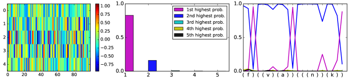
Figure 20: Visualization of a sr-LSTM-p with $k=5$ centroids, a hidden state dimension of $100$, trained on the large BP data. (Left) visualization of the learned centroids. (Center) mean transition probabilities when ranked highest to lowest. This shows that the transition probabilities are quite spiky. (Right) transition probabilities for a specific input sequence.

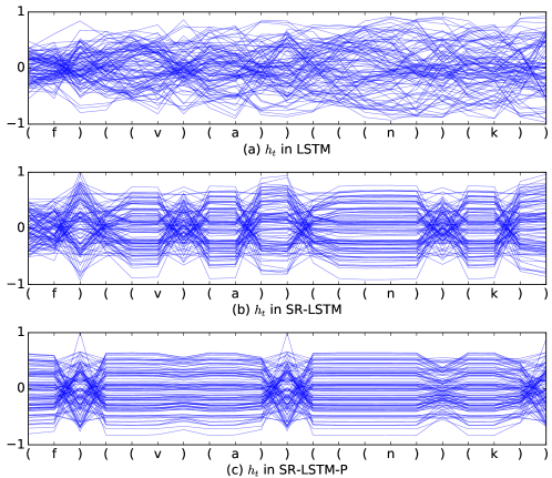
Figure 21: Visualizations of the hidden states $\mathbf{h}$ of a vanilla LSTM, an sr-LSTM, and a sr-LSTM-p ($k=10$) for a specific input sequence. All models were trained on BP and have hidden state dimension of $100$. The LSTM memorizes with its hidden state. The sr-LSTM and sr-LSTM-p utilize few states and have a more stable behavior over time.

Centroids	Top-5 words with probabilities
centroid 0	piece (0.465) instead (0.453) slow (0.453) surface (0.443) artificial (0.37)
centroid 1	told (0.752) mr. (0.647) their (0.616) she (0.584) though (0.561)
centroid 2	just (0.943) absolutely (0.781) extremely (0.708) general (0.663) sitting (0.587)
centroid 3	worst (1.0) bad (1.0) pointless (1.0) boring (1.0) poorly (1.0)
centroid 4	jean (0.449) bug (0.406) mind (0.399) start (0.398) league (0.386)
centroid 5	not (0.997) never (0.995) might (0.982) at (0.965) had (0.962)
centroid 6	against (0.402) david (0.376) to (0.376) saying (0.357) wave (0.349)
centroid 7	simply (0.961) totally (0.805) c (0.703) once (0.656) simon (0.634)
centroid 8	10 (0.994) best (0.992) loved (0.99) 8 (0.987) highly (0.987)
centroid 9	you (0.799) strong (0.735) magnificent (0.726) 30 (0.714) honest (0.69)

Table 6: List of prototypical words for the $k=10$ centroids of an sr-LSTM-p trained on the IMDB dataset. The top-5 highest transition probability words are listed for each centroid. We colored the positive centroid words in green and the negative centroid words in red.

G.1 Balanced Parentheses

Figure 19 presents the visualization of hidden state $\mathbf{h}_{t}$ and cell state $\mathbf{c}_{t}$ of the LSTM and the sr-LSTM-p for a specific input sequence from BP.

Figure 20 (left) shows the $k=5$ learned centroids of a sr-LSTM-p with hidden state dimension $100$.

Figure 20 (center) depicts the average of the ranked transition probabilities for a large number of input sequences. This shows that, on average, the transition probabilities are spiky, with the highest transition probability being on average $0.83$, the second highest $0.16$ and so on.

Figure 20 (right) plots the transition probabilities for a sr-LSTM-p with $k=5$ states and hidden state dimension $100$ for a specific input sequence of BP.

Figure 21 visualizes the hidden states $\mathbf{h}$ of a LSTM, sr-LSTM, and sr-LSTM-p trained on the large BP dataset. The sr-LSTM and sr-LSTM-p have $k=5$ centroids and a hidden state dimension of $100$. One can see that the LSTM memorizes with its hidden states. The evolution of its hidden states is highly irregular. The sr-LSTM and sr-LSTM-p, on the other hand, have a much more regular behavior. The sr-LSTM-p utilizes mainly two states to accept and reject an input sequence.

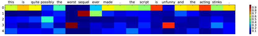
Figure 22: Visualization of the transition probabilities for an sr-LSTM-p with $k=5$ centroids trained on the IMDB dataset for a negative input sentence.

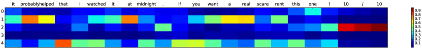
Figure 23: Visualization of the transition probabilities for an sr-LSTM-p with $k=5$ centroids trained on the IMDB dataset for a positive input sentence.

G.2 Sentiment Analysis

Since we can compute transition probabilities in each time step of an input sequence, we can use these probabilities to generate and visualize prototypical input tokens and the way that they are associated with certain centroids. We show in the following that it is possible to associate input tokens (here: words of reviews) to centroids by using their transition probabilities.

For the sentiment analysis data (IMDB) we can associate words to centroids for which they have high transition probabilities. To test this, we fed all test samples to a trained sr-LSTM-p. We determine the average transition probabilities for each word and centroid and select those words with the highest average transition probability to a centroid as the prototypical words of said centroid. Table 6 lists the top 5 words according to the transition probabilities to each of the 5 centroids for the sr-LSTM-p with $k=10$. It is now possible to inspect the words of each of the centroids to understand more about the working of the sr-RNN.

Figure 22 and 23 demonstrate that it is possible to visualize the transition probabilities for each input sequence. Here, we can see the transition probabilities for one positive and one negative sentence for a sr-LSTM-p with $k=5$ centroids.

In addition, sr-RNN can be used to visualize the transition probabilities for specific inputs. To explore this, we trained an sr-LSTM-p ($k=10$) on the MNIST (accuracy 98%) and Fashion MNIST (86%) data (Xiao et al., 2017), having the models process the images pixel-by-pixel as a large sequence.

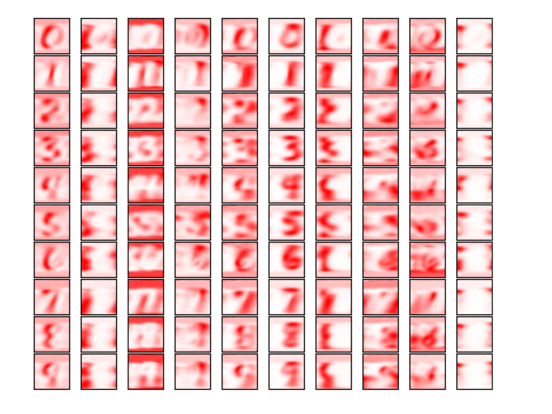
(a)

Figure 24: Visualization of average transition probabilities of the sr-LSTM-p with $k=10$ centroids, over all test images. Each row represents a digit class (a concept) and each column depicts the prototype (average transition probability) for each of the centroids.

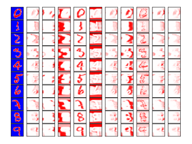
(a)

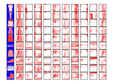
(b)

Figure 25: We can visualize the working of an sr-LSTM-p on a specific input image by visualizing the transition probabilities of each of the centroids (here: $k=10$). (Top) The visualizetion for some MNIST images. (Bottom) The visualization for some Fashion-MNIST images. The first column depicts the input image and the second to to $11^{th}$ the state transition probability heatmaps corresponding to the 10 centroids.

G.3 MNIST and Fashion-MNIST

For pixel-by-pixel sequences, we can use the sr-RNNs to directly generate prototypes that might assist in understanding the way sr-RNNs work. We can compute and visualize the average transition probabilities for all examples of a given class. Note that this is different to previous post-hoc methods (e.g., activation maximization (Berkes & Wiskott, 2006; Nguyen et al., 2016)), in which a network is trained first and in a second step a second neural network is trained to generate the prototypes.

Figure 24 visualizes the prototypes (average transition probabilities for all examples from a digit class) of sr-LSTM-p for $k=10$ centroids. One can see that each centroid is paying attention to a different part of the image.

Figure 25 visualizes the explanations that generated for RNN predictions with a given input of sr-LSTM-p for $k=10$ centroids. One can see that the important features are highlighted for explaining the predictions.

References

- Arjovsky et al. (2016) Arjovsky, M., Shah, A., and Bengio, Y. Unitary evolution recurrent neural networks. In ICML, pp. 1120–1128, 2016.
- Bahdanau et al. (2015) Bahdanau, D., Cho, K., and Bengio, Y. Neural machine translation by jointly learning to align and translate. ICLR, 2015.
- Bai et al. (2018) Bai, S., Kolter, J. Z., and Koltun, V. An empirical evaluation of generic convolutional and recurrent networks for sequence modeling. CoRR, abs/1803.01271, 2018. URL http://arxiv.org/abs/1803.01271.
- Bayer & Osendorfer (2014) Bayer, J. and Osendorfer, C. Learning stochastic recurrent networks. arXiv preprint arXiv:1411.7610, 2014.
- Berkes & Wiskott (2006) Berkes, P. and Wiskott, L. On the analysis and interpretation of inhomogeneous quadratic forms as receptive fields. Neural computation, 18(8):1868–1895, 2006.
- Campos et al. (2018) Campos, V., Jou, B., Giró-i Nieto, X., Torres, J., and Chang, S.-F. Skip rnn: Learning to skip state updates in recurrent neural networks. ICLR, 2018.
- Chang et al. (2017) Chang, S., Zhang, Y., Han, W., Yu, M., Guo, X., Tan, W., Cui, X., Witbrock, M., Hasegawa-Johnson, M. A., and Huang, T. S. Dilated recurrent neural networks. In NIPS, pp. 77–87, 2017.
- Chung et al. (2014) Chung, J., Gülçehre, Ç., Cho, K., and Bengio, Y. Empirical evaluation of gated recurrent neural networks on sequence modeling. arXiv e-prints, abs/1412.3555, 2014. Presented at the Deep Learning workshop at NIPS2014.
- Cooijmans et al. (2017) Cooijmans, T., Ballas, N., Laurent, C., Gülçehre, Ç., and Courville, A. Recurrent batch normalization. ICLR, 2017.
- Dahl et al. (2012) Dahl, G. E., Adams, R. P., and Larochelle, H. Training restricted boltzmann machines on word observations. ICML, 2012.
- Dai & Le (2015) Dai, A. M. and Le, Q. V. Semi-supervised sequence learning. In NIPS, pp. 3079–3087, 2015.
- Danihelka et al. (2016) Danihelka, I., Wayne, G., Uria, B., Kalchbrenner, N., and Graves, A. Associative long short-term memory. In International Conference on Machine Learning, pp. 1986–1994, 2016.
- Daniluk et al. (2017a) Daniluk, M., Rocktäschel, T., Welbl, J., and Riedel, S. Frustratingly short attention spans in neural language modeling. 2017a.
- Daniluk et al. (2017b) Daniluk, M., Rocktäschel, T., Welbl, J., and Riedel, S. Frustratingly short attention spans in neural language modeling. ICLR, 2017b.
- Dieng et al. (2018) Dieng, A. B., Ranganath, R., Altosaar, J., and Blei, D. M. Noisin: Unbiased regularization for recurrent neural networks. ICML, 2018.
- Elman (1990) Elman, J. L. Finding structure in time. Cognitive science, 14(2):179–211, 1990.
- Foerster et al. (2017) Foerster, J. N., Gilmer, J., Sohl-Dickstein, J., Chorowski, J., and Sussillo, D. Input switched affine networks: An rnn architecture designed for interpretability. In Proceedings of the 34th International Conference on Machine Learning-Volume 70, pp. 1136–1145. JMLR. org, 2017.
- Fraccaro et al. (2016) Fraccaro, M., Sø nderby, S. r. K., Paquet, U., and Winther, O. Sequential neural models with stochastic layers. In Advances in Neural Information Processing Systems, pp. 2199–2207. 2016.
- Frasconi & Bengio (1994) Frasconi, P. and Bengio, Y. An em approach to grammatical inference: input/output hmms. In Proceedings of 12th International Conference on Pattern Recognition, pp. 289–294. IEEE, 1994.
- Gal & Ghahramani (2016) Gal, Y. and Ghahramani, Z. A theoretically grounded application of dropout in recurrent neural networks. In Advances in neural information processing systems, pp. 1019–1027, 2016.
- Gers & Schmidhuber (2001) Gers, F. A. and Schmidhuber, E. Lstm recurrent networks learn simple context-free and context-sensitive languages. IEEE Transactions on Neural Networks, 12(6):1333–1340, 2001.
- Gers & Schmidhuber (2000) Gers, F. A. and Schmidhuber, J. Recurrent nets that time and count. In IJCNN (3), pp. 189–194, 2000.
- Giles et al. (1991) Giles, C. L., Chen, D., Miller, C., Chen, H., Sun, G., and Lee, Y. Second-order recurrent neural networks for grammatical inference. In Neural Networks, 1991., IJCNN-91-Seattle International Joint Conference on, volume 2, pp. 273–281. IEEE, 1991.
- Goyal et al. (2017) Goyal, A., Sordoni, A., Côté, M.-A., Ke, N., and Bengio, Y. Z-forcing: Training stochastic recurrent networks. In Guyon, I., Luxburg, U. V., Bengio, S., Wallach, H., Fergus, R., Vishwanathan, S., and Garnett, R. (eds.), Advances in Neural Information Processing Systems 30, pp. 6713–6723. 2017.
- Graves et al. (2014) Graves, A., Wayne, G., and Danihelka, I. Neural turing machines. arXiv preprint arXiv:1410.5401, 2014.
- Graves et al. (2016) Graves, A., Wayne, G., Reynolds, M., Harley, T., Danihelka, I., Grabska-Barwinska, A., Colmenarejo, S. G., Grefenstette, E., Ramalho, T., Agapiou, J., Badia, A. P., Hermann, K. M., Zwols, Y., Ostrovski, G., Cain, A., King, H., Summerfield, C., Blunsom, P., Kavukcuoglu, K., and Hassabis, D. Hybrid computing using a neural network with dynamic external memory. Nature, 538(7626):471–476, 2016.
- Grefenstette et al. (2015) Grefenstette, E., Hermann, K. M., Suleyman, M., and Blunsom, P. Learning to transduce with unbounded memory. In Advances in Neural Information Processing Systems, pp. 1828–1836, 2015.
- Hao et al. (2018) Hao, Y., Merrill, W., Angluin, D., Frank, R., Amsel, N., Benz, A., and Mendelsohn, S. Context-free transductions with neural stacks. In Proceedings of the Analyzing and Interpreting Neural Networks for NLP workshop at EMNLP, 2018.
- Hochreiter & Schmidhuber (1997) Hochreiter, S. and Schmidhuber, J. Long short-term memory. Neural Comput., 9(8):1735–1780, 1997.
- Jing et al. (2017) Jing, L., Shen, Y., Dubcek, T., Peurifoy, J., Skirlo, S., LeCun, Y., Tegmark, M., and Soljačić, M. Tunable efficient unitary neural networks (EUNN) and their application to RNNs. In Precup, D. and Teh, Y. W. (eds.), Proceedings of the 34th International Conference on Machine Learning, volume 70 of Proceedings of Machine Learning Research, pp. 1733–1741, International Convention Centre, Sydney, Australia, 06–11 Aug 2017. PMLR.
- Johnson & Zhang (2015) Johnson, R. and Zhang, T. Effective use of word order for text categorization with convolutional neural networks. NAACL HLT, 2015.
- Le et al. (2015) Le, Q. V., Jaitly, N., and Hinton, G. E. A simple way to initialize recurrent networks of rectified linear units. arXiv preprint arXiv:1504.00941, 2015.
- LeCun et al. (1998) LeCun, Y., Bottou, L., Bengio, Y., and Haffner, P. Gradient-based learning applied to document recognition. Proceedings of the IEEE, 86(11):2278–2324, 1998.
- Maas et al. (2011) Maas, A. L., Daly, R. E., Pham, P. T., Huang, D., Ng, A. Y., and Potts, C. Learning word vectors for sentiment analysis. In ACL-HLT, pp. 142–150, Portland, Oregon, USA, June 2011. Association for Computational Linguistics.
- Mensch & Blondel (2018) Mensch, A. and Blondel, M. Differentiable dynamic programming for structured prediction and attention. In Proceedings of the 35th International Conference on Machine Learning, volume 80, pp. 3462–3471, 2018.
- Merity et al. (2018) Merity, S., Keskar, N. S., and Socher, R. Regularizing and optimizing lstm language models. ICLR, 2018.
- Miller & Hardt (2018) Miller, J. and Hardt, M. When recurrent models don’t need to be recurrent. CoRR, abs/1805.10369, 2018.
- Murdoch & Szlam (2017) Murdoch, W. J. and Szlam, A. Automatic rule extraction from long short term memory networks. In ICLR, 2017.
- Nguyen et al. (2016) Nguyen, A., Dosovitskiy, A., Yosinski, J., Brox, T., and Clune, J. Synthesizing the preferred inputs for neurons in neural networks via deep generator networks. In Advances in Neural Information Processing Systems, pp. 3387–3395, 2016.
- Ostmeyer & Cowell (2017) Ostmeyer, J. and Cowell, L. Machine learning on sequential data using a recurrent weighted average. arXiv preprint arXiv:1703.01253, 2017.
- Schellhammer et al. (1998) Schellhammer, I., Diederich, J., Towsey, M., and Brugman, C. Knowledge extraction and recurrent neural networks: An analysis of an elman network trained on a natural language learning task. In Proceedings of the Joint Conferences on New Methods in Language Processing and Computational Natural Language Learning, pp. 73–78, 1998.
- Schmidhuber et al. (2002) Schmidhuber, J., Gers, F., and Eck, D. Learning nonregular languages: A comparison of simple recurrent networks and lstm. Neural Computation, 14(9):2039–2041, 2002.
- Siegelmann (2012) Siegelmann, H. T. Neural networks and analog computation: beyond the Turing limit. Springer Science & Business Media, 2012.
- Siegelmann & Sontag (1992) Siegelmann, H. T. and Sontag, E. D. On the computational power of neural nets. In Proceedings of the fifth annual workshop on Computational learning theory, pp. 440–449. ACM, 1992.
- Siegelmann & Sontag (1994) Siegelmann, H. T. and Sontag, E. D. Analog computation via neural networks. Theoretical Computer Science, 131(2):331–360, 1994.
- Soltani & Jiang (2016) Soltani, R. and Jiang, H. Higher order recurrent neural networks. arXiv preprint arXiv:1605.00064, 2016.
- Srivastava et al. (2014) Srivastava, N., Hinton, G., Krizhevsky, A., Sutskever, I., and Salakhutdinov, R. Dropout: a simple way to prevent neural networks from overfitting. The Journal of Machine Learning Research, 15(1):1929–1958, 2014.
- Strobelt et al. (2016) Strobelt, H., Gehrmann, S., Huber, B., Pfister, H., Rush, A. M., et al. Visual analysis of hidden state dynamics in recurrent neural networks. CoRR, abs/1606.07461, 2016.
- Theano Development Team (2016) Theano Development Team. Theano: A Python framework for fast computation of mathematical expressions. arXiv e-prints, abs/1605.02688, 2016.
- Tomita (1982) Tomita, M. Dynamic construction of finite automata from examples using hill-climbing. In Proceedings of the Fourth Annual Conference of the Cognitive Science Society, pp. 105–108, 1982.
- Tran et al. (2016) Tran, K., Bisazza, A., and Monz, C. Recurrent memory networks for language modeling. NAACL-HLT, 2016.
- Trinh et al. (2018) Trinh, T. H., Dai, A. M., Luong, T., and Le, Q. V. Learning longer-term dependencies in rnns with auxiliary losses. ICML, 2018.
- Vaswani et al. (2017) Vaswani, A., Shazeer, N., Parmar, N., Uszkoreit, J., Jones, L., Gomez, A. N., Kaiser, L. u., and Polosukhin, I. Attention is all you need. In Guyon, I., Luxburg, U. V., Bengio, S., Wallach, H., Fergus, R., Vishwanathan, S., and Garnett, R. (eds.), Advances in Neural Information Processing Systems, pp. 5998–6008. 2017.
- Wang et al. (2018a) Wang, Q., Zhang, K., Ororbia, I., Alexander, G., Xing, X., Liu, X., and Giles, C. L. A comparison of rule extraction for different recurrent neural network models and grammatical complexity. arXiv preprint arXiv:1801.05420, 2018a.
- Wang et al. (2018b) Wang, Q., Zhang, K., Ororbia II, A. G., Xing, X., Liu, X., and Giles, C. L. An empirical evaluation of rule extraction from recurrent neural networks. Neural Computation, 30(9):2568–2591, 2018b.
- Weiss et al. (2018a) Weiss, G., Goldberg, Y., and Yahav, E. On the practical computational power of finite precision rnns for language recognition. In Proceedings of the 56th Annual Meeting of the Association for Computational Linguistics (Volume 2: Short Papers), pp. 740–745, 2018a.
- Weiss et al. (2018b) Weiss, G., Goldberg, Y., and Yahav, E. Extracting automata from recurrent neural networks using queries and counterexamples. In Proceedings of the 35th International Conference on Machine Learning, volume 80, pp. 5247–5256, 2018b.
- Weston et al. (2015) Weston, J., Chopra, S., and Bordes, A. Memory networks. 2015.
- Wisdom et al. (2016) Wisdom, S., Powers, T., Hershey, J., Le Roux, J., and Atlas, L. Full-capacity unitary recurrent neural networks. In Lee, D. D., Sugiyama, M., Luxburg, U. V., Guyon, I., and Garnett, R. (eds.), NIPS, pp. 4880–4888. 2016.
- Xiao et al. (2017) Xiao, H., Rasul, K., and Vollgraf, R. Fashion-mnist: a novel image dataset for benchmarking machine learning algorithms. arXiv preprint arXiv:1708.07747, 2017.
- Yu et al. (2017) Yu, A. W., Lee, H., and Le, Q. V. Learning to skim text. ACL, 2017.
- Zaremba & Sutskever (2014) Zaremba, W. and Sutskever, I. Learning to execute. CoRR, abs/1410.4615, 2014.
- Zaremba et al. (2014) Zaremba, W., Sutskever, I., and Vinyals, O. Recurrent neural network regularization. arXiv preprint arXiv:1409.2329, 2014.
- Zeng et al. (1993) Zeng, Z., Goodman, R. M., and Smyth, P. Learning finite state machines with self-clustering recurrent networks. Neural Computation, 5(6):976–990, 1993.
- Zhang et al. (2016) Zhang, S., Wu, Y., Che, T., Lin, Z., Memisevic, R., Salakhutdinov, R. R., and Bengio, Y. Architectural complexity measures of recurrent neural networks. In Advances in Neural Information Processing Systems, pp. 1822–1830, 2016.
- Zilly et al. (2017) Zilly, J. G., Srivastava, R. K., Koutník, J., and Schmidhuber, J. Recurrent highway networks. In Proceedings of the 34th International Conference on Machine Learning-Volume 70, pp. 4189–4198. JMLR. org, 2017.