Unsupervised speech representation learning
using WaveNet autoencoders

Abstract

We consider the task of unsupervised extraction of meaningful latent representations of speech by applying autoencoding neural networks to speech waveforms. The goal is to learn a representation able to capture high level semantic content from the signal, e.g. phoneme identities, while being invariant to confounding low level details in the signal such as the underlying pitch contour or background noise. Since the learned representation is tuned to contain only phonetic content, we resort to using a high capacity WaveNet decoder to infer information discarded by the encoder from previous samples. Moreover, the behavior of autoencoder models depends on the kind of constraint that is applied to the latent representation. We compare three variants: a simple dimensionality reduction bottleneck, a Gaussian Variational Autoencoder (VAE), and a discrete Vector Quantized VAE (VQ-VAE). We analyze the quality of learned representations in terms of speaker independence, the ability to predict phonetic content, and the ability to accurately reconstruct individual spectrogram frames. Moreover, for discrete encodings extracted using the VQ-VAE, we measure the ease of mapping them to phonemes. We introduce a regularization scheme that forces the representations to focus on the phonetic content of the utterance and report performance comparable with the top entries in the ZeroSpeech 2017 unsupervised acoustic unit discovery task.

I Introduction

Creating good data representations is important. The deep learning revolution was triggered by the development of hierarchical representation learning algorithms, such as stacked Restricted Boltzman Machines [1] and Denoising Autoencoders [2]. However, recent breakthroughs in computer vision [3, 4], machine translation [5, 6], speech recognition [7, 8], and language understanding [9, 10] rely on large labeled datasets and make little to no use of unsupervised representation learning. This has two drawbacks: first, the requirement of large human labeled datasets often makes the development of deep learning models expensive. Second, while a deep model may excel at solving a given task, it yields limited insights into the problem domain, with main intuitions typically consisting of visualizations of salient input patterns [11, 12], a strategy that is applicable only to problem domains that are easily solved by humans.

In this paper we focus on evaluating and improving unsupervised speech representations. Specifically, we focus on representations that separate selected speaker traits, specifically speaker gender and identity, from phonetic content, properties which are consistent with internal representations learned by speech recognizers [13, 14]. Such representations are desired in several tasks, such as low resource automatic speech recognition (ASR), where only a small amount of labeled training data is available. In such scenario, limited amounts of data may be sufficient to learn an acoustic model on the representation discovered without supervision, but insufficient to learn the acoustic model and a data representation in a fully supervised manner [15, 16].

We focus on representations learned with autoencoders applied to raw waveforms and spectrogram features and investigate the quality of learned representations on LibriSpeech [17]. We tune the learned latent representation to encode only phonetic content and remove other confounding detail. However, to enable signal reconstruction, we rely on an autoregressive WaveNet [18] decoder to infer information that was rejected by the encoder. The use of such a powerful decoder acts as an inductive bias, freeing up the encoder from using its capacity to represent low level detail and instead allowing it to focus on high level semantic features. We discover that best representations arise when ASR features, such as mel-frequency cepstral coefficients (MFCCs) are used as inputs, while raw waveforms are used as decoder targets. This forces the system to also learn to generate sample level detail which was removed during feature extraction. Furthermore, we observe that the Vector Quantized Variational Autoencoder (VQ-VAE) [19] yields the best separation between the acoustic content and speaker information. We investigate the interpetability of VQ-VAE tokens by mapping them to phonemes, demonstrate the impact of model hyperparameters on interpretability and propose a new regularization scheme which improves the degree to which the latent representation can be mapped to the phonetic content. Finally, we demonstrate strong performance on the ZeroSpeech 2017 acoustic unit discovery task [20], which measures how discriminative a representation is to minimal phonetic changes within an utterance.

II Representation Learning with Neural Networks

Neural networks are hierarchical information processing models that are typically implemented using layers of computational units. Each layer can be interpreted as a feature extractor whose outputs are passed to upstream units [21]. Especially in the visual domain, features learned with neural networks have been shown to create a hierarchy of visual atoms [11] that match some properties of the visual cortex [22]. Similarly, when applied to audio waveforms, neural networks have been shown to learn auditory-like frequency decompositions on music [23] and speech [24, 25, 26, 27] in their lower layers.

II-A Supervised feature learning

Neural networks can learn useful data representations in both supervised and unsupervised manners. In the supervised case, features learned on large datasets are often directly useful in similar but data-poor tasks. For instance, in the visual domain, features discovered on ImageNet [28] are routinely used as input representations in other computer vision tasks [29]. Similarly, the speech community has used bottleneck features extracted from networks trained on phoneme prediction tasks [30, 31] as feature representations for speech recognition systems. Likewise, in natural language processing, universal text representations can be extracted from networks trained for machine translation [32] or language inference [33, 34].

II-B Unsupervised feature learning

In this paper we focus on unsupervised feature learning. Since no training labels are available we investigate autoencoders, i.e., networks which are tasked with reconstructing their inputs. Autoencoders use an encoding network to extract a latent representation, which is then passed through a decoding network to recover the original data. Ideally, the latent representation preserves the salient features of the original data, while being easier to analyze and work with, e.g. by disentangling different factors of variation in the data, and discarding spurious patterns (noise). These desirable qualities are typically obtained through a judicious application of regularization techniques and constraints or bottlenecks (we use the two terms interchangeably). The representation learned by an autoencoder is thus subject to two competing forces. On the one hand, it should provide the decoder with information necessary for perfect reconstruction and thus capture in the latents as much of the input data characteristics as possible. On the other hand, the constraints force some information to be discarded, preventing the latent representation from being trivial to invert, e.g. by exactly passing through the input. Thus the bottleneck is necessary to force the network to learn a non-trivial data transformation.

Reducing the dimensionality of the latent representation can serve as a basic constraint applied to the latent vectors, with the autoencoder acting as a nonlinear variant of linear low-rank data projections, such as PCA or SVD [35]. However, such representations may be difficult to interpret because the reconstruction of an input depends on all latent features [36]. In contrast, dictionary learning techniques, such as sparse [37] and non-negative [36] decompositions, express each input pattern using a combination of a small number of selected features out of a larger pool, which facilitates their interpretability. Discrete feature learning using vector quantization can be seen as an extreme form of sparseness in which the reconstruction uses only one element from the dictionary.

The Variational Autoencoder (VAE) [38] proposes a different interpretation of feature learning which follows a probabilistic framework. The autoencoding network is derived from a latent-variable generative model. First, a latent vector $z$ is sampled from a prior distribution $p(z)$ (typically a multidimensional normal distribution). Then the data sample $x$ is generated using a deep decoder neural network with parameters $\theta$ that computes $p(x|z;\theta)$. However, computing the exact posterior distribution $p(z|x)$ that is needed during maximum likelihood training is difficult. Instead, the VAE introduces a variational approximation to the posterior, $q(z|x;\phi)$, which is modeled using an encoder neural network with parameters $\phi$. Thus the VAE resembles a traditional autoencoder, in which the encoder produces distributions over latent representations, rather than deterministic encodings, while the decoder is trained on samples from this distribution. Encoding and decoding networks are trained jointly to maximize a lower bound on the log-likelihood of data point $x$ [38, 39]:

$$J_{\mathit{VAE}}(\theta,\phi;x)=\, \mathbb{E}_{q(z|x;\phi)}\left[\log p(x|z;\theta)\right]-$$

$$\beta\,D_{KL}\left(q(z|x;\phi)\,||\,p(z)\right).$$ (1)

We can interpret the two terms of Eq. (II-B) as the autoencoder’s reconstruction cost augmented with a penalty term applied to the hidden representation. In particular, the KL divergence expresses the amount of information in nats which the latent representation carries about the data sample. Thus, it acts as an information bottleneck [40] on the latent representation, where $\beta$ controls the trade-off between reconstruction quality and the representation simplicity.

An alternative formulation of the VAE objective explicitly constrains the amount of information contained in the latent representation [41]:

$$J_{\mathit{VAE}}(\theta,\phi;x)=\, \mathbb{E}_{q(z|x;\phi)}\left[\log p(x|z;\theta)\right]-$$

$$\max\left(B,D_{KL}\left(q(z|x;\phi)\,||\,p(z)\right)\right),$$ (2)

where the constant $B$ corresponds to the amount of free information in $q$, because the model is only penalized if it transmits more than $B$ nats over the prior in the distribution over the latents. Please note that for convenience we will often refer to information content using units of bits instead of nats.

A recently proposed modification of the VAE, called the Vector Quantized VAE [19], replaces the continuous and stochastic latent vectors with deterministically quantized versions. The VQ-VAE maintains a number of prototype vectors $\{e_{i},i=1,\ldots,K\}$. During the forward pass, representations produced by the encoder are replaced with their closest prototypes. Formally, let $z_{e}(x)$ be the output of the encoder prior to quantization. VQ-VAE finds the nearest prototype $q(x)=\text{argmin}_{i}\|z_{e}(x)-e_{i}\|_{2}^{2}$ and uses it as the latent representation $z_{q}(x)=e_{q(x)}$ which is passed to the decoder. When using the model in downstream tasks, the learned representation can therefore be treated either as a distributed representation in which each sample is represented by a continuous vector, or as a discrete representation in which each sample is represented by the prototype ID (also called the token ID).

During the backward pass, the gradient of the loss with respect to the pre-quantized embedding is approximated using the straight-through estimator [42], i.e., $\frac{\partial\mathcal{L}}{\partial z_{e}(x)}\approx\frac{\partial\mathcal{L}}{\partial z_{q}(x)}$. The prototypes are trained by extending the learning objective with terms which optimize quantization. Prototypes are forced to lie close to vectors which they replace with an auxiliary cost, dubbed the commitment loss, introduced to encourage the encoder to produce vectors which lie close to prototypes. Without the commitment loss VQ-VAE training can diverge by emitting representations with unbounded magnitude. Therefore, VQ-VAE is trained using a sum of three loss terms: the negative log-likelihood of the reconstruction, which uses the straight-through estimator to bring the gradient from the decoder to the encoder, and two VQ-related terms: the distance from each prototype to its assigned vectors and the commitment cost [19]:

$$\mathcal{L}=\, \log p\big{(}x\mid z_{q}(x)\big{)}$$

$$+\|\text{sg}\big{(}z_{e}(x)\big{)}-e_{q(x)}\|^{2}_{2}+\gamma\|z_{e}(x)-\text{sg}(e_{q(x)})\|_{2}^{2},$$ (3)

where $\text{sg}(\cdot)$ denotes the stop-gradient operation which zeros the gradient with respect to its argument during backward pass.

The quantization within the VQ-VAE acts as an information bottleneck. The encoder can be interpreted as a probabilistic model which puts all probability mass on the selected discrete token (prototype ID). Assuming a uniform prior distribution over $K$ tokens, the KL divergence is constant and equal to $\log K$. Therefore, the KL term does not need to be included in the VQ-VAE training criterion in Eq. (II-B) and instead becomes a hyperparameter tied to the size of the prototype inventory.

The VQ-VAE was qualitatively shown to learn a representation which separated the phonetic content within an utterance from the identity of the speaker [19]. Moreover the discovered tokens could be mapped to phonemes in a limited setting.

II-C Autoencoders for sequential data

Sequential data, such as speech or text, often contain local dependencies that can be exploited by generative models. In fact, purely autoregressive models of sequential data, which predict the next observation based on recent history, are very successful. For text, these correspond to $n$-gram models [43] and convolutional neural language models [44, 45]. Similarly, WaveNet [18] is a state-of-the-art autoregressive model of time-domain waveform samples for text-to-speech synthesis.

Figure 1: The proposed model is conceptually divided into 3 parts: an encoder (green), made of a residual convnet that computes a stream of latent vectors (typically every 10ms or 20ms) from a time-domain waveform sampled at 16 kHz, which are passed through a bottleneck (red) before being used to condition a WaveNet decoder (blue) which reconstructs the waveform using two additional information streams: an autoregressive stream which predicts the next sample based on past samples, and global conditioning which represents the identity of the input speaker (one out of $N_{s}$ total training speakers). We experiment with three bottleneck variants: a simple dimensionality reduction (AE), a sampling layer with an additional Kullback-Leibler penalty term (VAE), or a discretization layer (VQ-VAE). Intuitively, this bottleneck encourages the encoder to discard portions of the latent representation which the decoder can infer from the two other information streams. For all layers, numbers in parentheses indicate the number of output channels, and subscripts denote the filter length. Locations of “probe” points which are used in Section IV to evaluate the quality of the learned representation are denoted with black dots.

A downside of such autoregressive models is that they do not explicitly produce latent representations of the data. However, it is possible to combine an autoregressive sequence generation model with an encoder tasked with extraction of latent representations. Depending on the use case, the encoder can process the whole utterance, emit a single latent vector and feed it to an autoregressive decoder [33, 46] or the encoder can periodically emit vectors of latent features to be consumed by the decoder [19, 47]. We concentrate on the latter solution.

Training mixed latent variable and autoregressive models is prone to latent space collapse, in which the decoder learns to ignore the constrained latent representations and only uses the unconstrained signal coming through the autoregressive path. For the VAE, this collapse can be prevented by annealing the weight of the KL term and using the free-information formulation in Eq. (II-B). The VQ-VAE is naturally resilient to the latent collapse because the KL term is a hyperparameter which is not optimized using gradient training of a given model. We defer further discussion of this topic to Section V.

III Model Description

The architecture of our model is presented in Figure 1. The encoder reads a sequence of either raw audio samples, or of audio features and extracts a sequence of hidden vectors, which are passed through a bottleneck to become a sequence of latent representations. The frequency at which the latent vectors are extracted is governed by the number of strided convolutions applied by the encoder.

The decoder reconstructs the utterance by conditioning a WaveNet [18] network on the latent representation extracted by the encoder and, separately, on a speaker embedding. Explicitly conditioning the decoder on speaker identity frees the encoder from having to capture speaker-dependent information in the latent representation. Specifically, the decoder (i) takes the encoder’s output, (ii) optionally applies a stochastic regularization to the latent vectors (see Section III-A), (iii) then combines latent vectors extracted at neighboring time steps using convolutions and (iv) upsamples them to the output frequency. Waveform samples are reconstructed with a WaveNet that combines all conditioning sources: autoregressive information about past samples, global information about the speaker, and latent information about past and future samples extracted by the encoder. We find that the encoder’s bottleneck and the proposed regularization is crucial in extracting nontrivial representations of data. With no bottleneck, the model is prone to learn a simple reconstruction strategy which makes verbatim copies of future samples. We also note that the encoder is speaker independent and requires only speech data, while the decoder also requires speaker information.

We consider three forms of bottleneck: (i) simple dimensionality reduction, (ii) a Gaussian VAE with different latent representation dimensionalities and different capacities following Eq. (II-B), and (iii) a VQ-VAE with different number of quantization prototypes. All bottlenecks are optionally followed by the dropout inspired time-jitter regularization described below. Furthermore, we experiment with different input and output representations, using raw waveforms, log-mel filterbank, and mel-frequency cepstral coefficient (MFCC) features which discard pitch information present in the spectrogram.

III-A Time-jitter regularization

We would like the model to learn a representation of speech which corresponds to the slowly-changing phonetic content within an utterance: a mostly constant signal that can abruptly change at phoneme boundaries.

Inspired by the slow features analysis [48] we first experimented with penalizing time differences between encoder representation either before or after the bottleneck. However, this regularization resulted in a collapse of the latent space – the model learned to output a constant encoding. This is a common problem of sequential VAEs that use loss terms to regularize the latent encoding [49].

Reconsidering the problem we realized that we want each frame’s representation to correspond to a meaningful phonetic unit. Thus we want to prevent the system from using consecutive latent vectors as individual units. Put differently, we want to prevent latent vector co-adaptation. We therefore introduce a dropout-inspired [50] time-jitter regularizer, also reminiscent of Zoneout [51] regularization for recurrent networks. During training, each latent vector can replace either one or both of its neighbors. As in dropout, this prevents the model from relying on consistency across groups of tokens. Additionally, this regularization also promotes latent representation stability over time: a latent vector extracted at time step $t$ must strive to also be useful at time steps $t-1$ or $t+1$. In fact, the regularization was crucial for reaching good performance on ZeroSpeech at higher token extraction frequencies.

The regularization layer is inserted right after the encoder’s bottleneck (i.e., after dimensionality reduction for regular autoencoder, after sampling a realization of the latent layer for the VAE and after discretization for the VQ-VAE). It is only enabled during training. For each time step we independently sample whether it is to be replaced with the token right after or before it. We do not copy a token more than one timestep.

IV Experiments

We evaluated models on two datasets: LibriSpeech [17] (clean subset) and ZeroSpeech 2017 Contest Track 1 data [20]. Both datasets have similar characteristics: multiple speakers, clean, read speech (sourced from audio books) recorded at a sampling rate of 16 kHz. Moreover the ZeroSpeech challenge controls the amount of per-speaker data with the majority of the data being uttered by only a few speakers.

Initial experiments, presented in section IV-B, compare different bottleneck variants and establish what type of information from the input audio is preserved in the continuous latent representations produced by the model at the four different probe points pictured in Figure 1. Using the representation computed at each probe point, we measure performance on several prediction tasks: phoneme prediction (per-frame accuracy), speaker identity and gender prediction accuracy, and $L_{2}$ reconstruction error of spectrogram frames. We establish that the VQ-VAE learns latent representations with strongest disentanglement between the phonetic content and speaker identity, and focus on this architecture in the following experiments.

In section IV-C we analyze the interpretability of VQ-VAE tokens by mapping each discrete token to the most frequent corresponding phoneme in a forced alignment of a small labeled data set (LibriSpeech dev) and report the accuracy of the mapping on a separate set (LibriSpeech test). Intuitively, this captures the interpretability of individual tokens.

We then apply the VQ-VAE to the ZeroSpeech 2017 acoustic unit discovery task [20] in section IV-D. This task evaluates how discriminative the representation is with respect to the phonetic class. Finally, in section IV-E we measure the impact of different hyperparameters on performance.

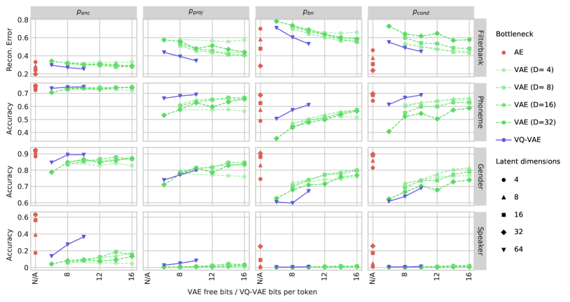
Figure 2: Accuracy of predicting signal characteristics at various probe locations in the network. Among the three bottlenecks evaluated, VQ-VAE discards the most speaker-related information at the bottleneck, while preserving the most phonetic information. For all bottlenecks, the representation coming out of the encoder yields over 70% accurate framewise phoneme predictions. Both the simple AE and VQ-VAE preserve this information in the bottleneck (the accuracy drops to 50%-60% depending on the bottleneck’s strength). However, the VQ-VAE discards almost all speaker information (speaker classification accuracy is close to 0% and gender prediction close to 50%). This causes the VQ-VAE representation to perform best on the acoustic unit discovery task – the representation captures the phonetic content while being invariant to speaker identity.

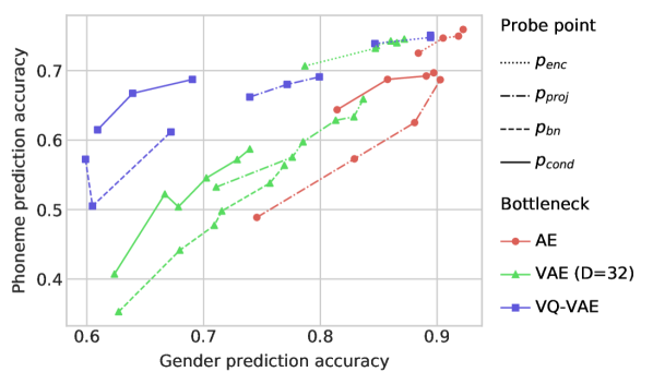
Figure 3: Comparison of gender and phoneme prediction accuracy for different bottleneck types and probe points. The decoder is conditioned on the speaker, thus the gender information can be recovered and the bottleneck should discard it. While information is present at the $p_{\text{enc}}$ probe. The AE and VAE models tend to similarly discard both gender and phoneme information at other probe points. On the other hand, VQ-VAE selectively discards gender information.

IV-A Default model hyperparameters

Our best models used MFCCs as the encoder input, but reconstructed raw waveforms at the decoder output. We used standard 13 MFCC features extracted every 10ms (i.e., at a rate of 100 Hz) and augmented with their temporal first and second derivatives. Such features were originally designed for speech recognition and are mostly invariant to pitch and similar confounding detail in the audio signal. The encoder had 9 layers each using 768 units with ReLU activation, organized into the following groups: 2 preprocessing convolution layers with filter length 3 and residual connections, 1 strided convolution length reduction layer with filter length 4 and stride 2 (downsampling the signal by a factor of two), followed by 2 convolutional layers with length 3 and residual connections, and finally 4 feedforward ReLU layers with residual connections. The resulting latent vectors were extracted at 50 Hz (i.e., every second frame), with each latent vector depending on a receptive field of 16 input frames. We also used an alternative encoder with two length reduction layers, which extracted latent representation at 25 Hz with a receptive field of 30 frames.

When unspecified, the latent representation was 64 dimensional and when applicable constrained to 14 bits. Furthermore, for the VQ-VAE we used the recommended $\gamma=0.25$ [19].

The decoder applied the randomized time-jitter regularization (see Section III-A). During training each latent vector was replaced with either of its neighbors with probability 0.12. The jittered latent sequence was passed through a single convolutional layer with filter length 3 and 128 hidden units to mix information across neighboring timesteps. The representation was then upsampled 320 times (to match the 16kHz audio sampling rate) and concatenated with a one-hot vector representing the current speaker to form the conditioning input of an autoregressive WaveNet [18]. The WaveNet was composed of 20 causal dilated convolution layers, each using 368 gated units with residual connections, organized into two “cycles” of 10 layers with dilation rates $1,2,4,\ldots,2^{9}$. The conditioning signal was passed separately into each layer. The signal from each layer of the WaveNet was passed to the output using skip-connections. Finally, the signal was passed through 2 ReLU layers with 256 units. A Softmax was applied to compute the next sample probability. We used 256 quantization levels after mu-law companding [18].

All models were trained on minibatches of 64 sequences of length 5120 time-domain samples (320 ms) sampled uniformly from the training dataset. Training a single model on 4 Google Cloud TPUs (16 chips) took a week. We used the Adam optimizer [52] with initial learning rate $4\times 10^{-4}$ which was halved after 400k, 600k, and 800k steps. Polyak averaging [53] was applied to all checkpoints used for model evaluation.

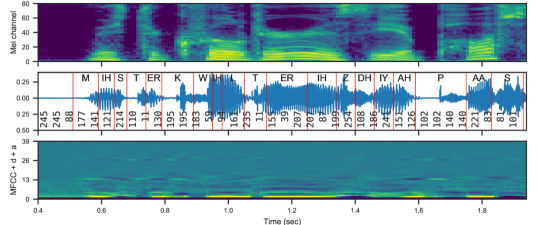
Figure 4: Example token sequence extracted by the proposed VQ-VAE model. Bottom: input MFCC features. Middle: Target waveform samples overlaid with extracted token IDs (bottom), and ground truth phoneme identities (top) with boundaries between plotted in red. Note the transient “T” phoneme at 0.75 and 1.1 seconds is consistently associated with token 11. The corresponding log-mel spectrogram is shown on the top.

IV-B Bottleneck comparison

We train models on LibriSpeech and analyze the information captured in the hidden representations surrounding the autoencoder bottleneck at each of the four probe points shown in Figure 1:

• $p_{\text{enc}}$ (768 dim) encoder output prior to the bottleneck,

• $p_{\text{proj}}$ (64 dim) within the bottleneck after projecting to lower dimension,

• $p_{\text{bn}}$ (64 dim) bottleneck output, corresponding to the quantized representation in VQ-VAE, or a random sample from the variational posterior in VAE, and

• $p_{\text{cond}}$ (128 dim) after passing $p_{\text{bn}}$ through a convolution layer which captures a larger receptive field over the latent encoding.

At each probe point, we train separate MLP networks with 2048 hidden units on each of four tasks: classifying speaker gender and identity for the whole segment (after average pooling latent vectors across the full signal), predicting phoneme class at each frame (making several predictions per latent vector), and reconstructing log-mel filterbank features in each frame (again predicting several consecutive frames from each latent vector). A representation which captures the high level semantic content from the signal, while being invariant to nuisance low-level signal details, will have a high phoneme prediction accuracy, and high spectrogram reconstruction error. A disentangled representation should additionally have low speaker prediction accuracy, since this information is explicitly made available to the decoder conditioning network, and therefore need not be preserved in the latent encoding [54]. Since we are primarily interested in discovering what information is present in the constructed representations we report the training performance and do not tune probing networks for generalization.

A comparison of models using each of the three bottlenecks with different hyperparameters (latent dimensionality and bottleneck bitrate) is presented in Figure 2, illustrating the degree of information propagation through the network. In addition, Figure 3, highlights the separation of phonetic content and speaker identity obtained using different configurations.

Figure 2 shows that each bottleneck type consistently discards information between the $p_{\text{enc}}$ and $p_{\text{bn}}$ probe locations, as evidenced by the reduced performance on each task. The bottleneck also impacts information content in preceding layers. Especially for the vanilla autoencoder (AE), which simply reduces dimensionality, the speaker prediction accuracy and filterbank reconstruction loss at $p_{\text{enc}}$ depend on the width of the bottleneck, with narrower widths causing more information to be discarded in lower layers of the encoder. Likewise, VQ-VAEs and AEs yielded better filterbank reconstructions and speaker identity prediction at $p_{\text{enc}}$ compared to VAEs with matching dimensionality and bitrate, which corresponds to the logarithm of the number of tokens for the VQ-VAE, and the KL divergence from the prior for the VAE, which we control by setting the number of allowed free bits.

As expected, AE discards the least information. At $p_{\text{cond}}$ the representation remains highly predictive about both speaker and phonemes, and its filterbank reconstructions are the best among all configurations. However, from an unsupervised learning standpoint, the AE latent representation is less useful because it mixes all properties of the source signal.

In contrast, VQ-VAE models produce a representation which is highly predictive of the phonetic content of the signal while effectively discarding speaker identity and gender information. At higher bitrates, phoneme prediction is about as accurate as for the AE. Filterbank reconstructions are also less accurate. We observe that the speaker information is discarded primarily during the quantization step between $p_{\text{proj}}$ and $p_{\text{bn}}$. Combining several latent vectors in the $p_{\text{cond}}$ representation results in more accurate phoneme predictions, but the additional context does not help to recover speaker information. This phenomenon is highlighted in Figure 3. Note that VQ-VAE models showed little dependence on the bottleneck dimension, so we present results at the default setting of 64.

Finally, VAE models separate speaker and phonetic information better than simple dimensionality reduction, but not as well as VQ-VAE. The VAE discards phonetic and speaker information more uniformly than VQ-VAE: at $p_{\text{bn}}$, VAE’s phoneme predictions are less accurate, while its gender predictions are more accurate. Moreover, combining information across a wider receptive field at $p_{\text{cond}}$ does not improve phoneme recognition as much as in VQ-VAE models. The sensitivity to the bottleneck dimensionality, seen in Figure 2 is also surprising, with narrower VAE bottlenecks discarding less information than wider ones. This may be due to the stochastic operation of the VAE: to provide the same KL divergence as at low bottleneck dimensions, more noise needs to be added at high dimensions. This noise may mask information present in the representation.

Based on these results we conclude that the VQ-VAE bottleneck is most appropriate for learning latent representations which capture phonetic content while being invariant to the underlying speaker identity.

IV-C VQ-VAE token interpretability

Up to this point we have used the VQ-VAE as a bottleneck that quantizes latent vectors. In this section we seek an interpretation of the discrete prototype IDs, evaluating whether VQ-VAE tokens can be mapped to phonemes, the underlying discrete constituents of speech sounds. Example token IDs are pictured in the middle pane of Figure 4, where we can see that the token 11 is consistently associated with the transient “T” phone. To evaluate whether other tokens have similar interpretations, we measured the frame-wise phoneme recognition accuracy in which each token was mapped to one out of 41 phonemes. We used the 460 hour clean LibriSpeech training set for unsupervised training, and used labels from the clean dev subset to associate each token with the most probable phoneme. We evaluated the mapping by computing frame-wise phone recognition accuracy on the clean test set at a frame rate of 100 Hz. The ground-truth phoneme boundaries were obtained from forced alignments using the Kaldi tri6b model from the s5 LibriSpeech recipe [55].

TABLE I: LibriSpeech frame-wise phoneme recognition accuracy. VQ-VAE models consume MFCC features and extracted tokens at 25 Hz.

	Num tokens / bits
	256	512	1024	2048	4096	8192	16384	32768
Train steps	8	9	10	11	12	13	14	15
200k	56.7	58.3	59.7	60.3	60.7	61.2	61.4	61.7
900k	58.6	61.0	61.9	63.3	63.8	63.9	64.3	64.5

Table I shows performance of the configuration which obtained the best accuracy mapping VQ-VAE tokens to phonemes on LibriSpeech. Recognition accuracy is given at two time points: after 200k gradient descent steps, when the relative performance of models can be assessed, and after 900k steps when the models have converged. We did not observe overfitting with longer training times. Predicting the most frequent silence phoneme for all frames set an accuracy lower bound at 16%. A model discriminatively trained on the full 460 hour training set to predict phonemes with the same architecture as the 25 Hz encoder achieved 80% framewise phoneme recognition accuracy, while a model with no time-reduction layers set the upper bound at 88%.

Table I indicates that the mapping accuracy improves with the number of tokens, with the best model reaching $64.5\%$ accuracy using 32768 tokens. However, the largest accuracy gain occurs at 4096 tokens, with diminishing returns as the number of tokens is further increased. This result is in rough correspondence with the 5760 tied triphone states used in the Kaldi tri6b model.

We also note that increasing the number of tokens does not trivially lead to improved accuracies, because we measure generalization, and not cluster purity. In the limit of assigning a different token to each frame, the accuracy will be poor because of overfitting to the small development set on which we establish the mapping. However, in our experiments we consistently observed improved accuracy.

IV-D Unsupervised ZeroSpeech 2017 acoustic unit discovery

The ZeroSpeech 2017 phonetic unit discovery task [20] evaluates a representation’s ability to discriminate between different sounds, rather than the ease of mapping the representation to predefined phonetic units. It is therefore complementary to the phoneme classification accuracy metric used in the previous section. The ZeroSpeech evaluation scheme uses the minimal pair ABX test [56, 57] which assesses the model’s ability to discriminate between pairs of three phoneme long segments of speech that differ only in the middle phone (e.g. “get” and “got”). We trained the models on the provided training data (45 hours for English, 24 hours for French and 2.5 hours for Mandarin) and evaluated them on the test data using the official evaluation scripts. To ensure that we do not overfit to the ZeroSpeech task we only considered the best hyperparameter settings found on LibriSpeech (c.f. Section IV-E). Moreover, to maximally abide by the ZeroSpeech convention, we used the same hyperparameters for all languages, denoted as VQ-VAE (per lang, MFCC, $p_{\text{cond}}$) in Table II.

TABLE II: ZeroSpeech 2017 phonetic unit discovery ABX scores reported across- and within-speakers (lower is better). The VQ-VAE encoder is speaker independent and thus its results do not change with the amount of test speaker data (1s, 10s, or 2m), while speaker-adaptive models (e.g. supervised topline) improve with more target speaker data. We report the two reference points from the challenge, along with the challenge winner [58] and three other submissions that used neural network in an unsupervised setting [59, 60, 61]. All VQ-VAE models use exactly the same hyperparameter setup (14 bit tokens extracted at 50 Hz with time-jitter probability 0.5), regardless of the amount of unlabeled training data (45h, 24h or 2.4h).The top VQ-VAE results row (VQ-VAE trained on target language, features extracted at the $p_{\text{cond}}$ point) gives best results overall. We also include in italics results for different probe points and for VQ-VAEs jointly trained on all languages. Multilingual training helps Mandarin. We also observe that the quantization mostly discards speaker and context influence. The context is however recovered in the conditioning signal which combines information from latent vectors at neighboring timesteps.

	Within-speaker											Across-speaker
	English (45h)				French (24h)				Mandarin (2.4h)				English (45h)				French (24h)				Mandarin (2.4h)
Model	1s	10s	2m		1s	10s	2m		1s	10s	2m		1s	10s	2m		1s	10s	2m		1s	10s	2m
Unsupervised baseline	12.0	12.1	12.1		12.5	12.6	12.6		11.5	11.5	11.5		23.4	23.4	23.4		25.2	25.5	25.2		21.3	21.3	21.3
Supervised topline	6.5	5.3	5.1		8.0	6.8	6.8		9.5	4.2	4.0		8.6	6.9	6.7		10.6	9.1	8.9		12.0	5.7	5.1
VQ-VAE (per lang, MFCC, $p_{\text{cond}}$)	5.6	5.5	5.5		7.3	7.5	7.5		11.2	10.7	10.8		8.1	8.0	8.0		11.0	10.8	11.1		12.2	11.7	11.9
VQ-VAE (per lang, MFCC, $p_{\text{bn}}$)	6.2	6.0	6.0		7.5	7.3	7.6		10.8	10.5	10.6		8.9	8.8	8.9		11.3	11.0	11.2		11.9	11.4	11.6
VQ-VAE (per lang, MFCC, $p_{\text{proj}}$)	5.9	5.8	5.9		6.7	6.9	6.9		9.9	9.7	9.7		9.1	9.0	9.0		11.9	11.6	11.7		11.0	10.6	10.7
VQ-VAE (all lang, MFCC, $p_{\text{cond}}$)	5.8	5.8	5.8		8.0	7.9	7.8		9.2	9.1	9.2		8.8	8.6	8.7		11.8	11.6	11.6		10.3	10.0	9.9
VQ-VAE (all lang, MFCC, $p_{\text{bn}}$)	6.3	6.2	6.3		8.0	8.0	7.9		9.0	8.9	9.1		9.4	9.2	9.3		11.8	11.7	11.8		9.9	9.7	9.7
VQ-VAE (all lang, MFCC, $p_{\text{proj}}$)	5.8	5.7	5.8		7.1	7.0	6.9		7.4	7.2	7.1		9.3	9.3	9.3		11.9	11.4	11.6		8.6	8.5	8.5
VQ-VAE (all lang, fbank, $p_{\text{proj}}$)	6.0	6.0	6.0		6.9	6.8	6.8		6.8	6.6	6.6		10.1	10.1	10.1		12.5	12.2	12.3		7.8	7.7	7.7
Heck et al. [58]	6.9	6.2	6.0		9.7	8.7	8.4		8.8	7.9	7.8		10.1	8.7	8.5		13.6	11.7	11.3		8.8	7.4	7.3
Chen et al. [59]	8.5	7.3	7.2		11.2	9.4	9.4		10.5	8.7	8.5		12.7	11.0	10.8		17.0	14.5	14.1		11.9	10.3	10.1
Ansari et al. [60]	7.7	6.8	N/A		10.4	N/A	8.8		10.4	9.3	9.1		13.2	12.0	N/A		17.2	N/A	15.4		13.0	12.2	12.3
Yuan et al. [61]	9.0	7.1	7.0		11.9	9.5	9.5		11.1	8.5	8.2		14.0	11.9	11.7		18.6	15.5	14.9		12.7	10.8	10.7

On English and French, which come with sufficiently large training datasets, we achieve results better than the top contestant [58], despite using a speaker independent encoder.

The results are consistent with our analysis of information separation performed by the VQ-VAE bottleneck: in the more challenging across-speaker evaluation, the best performance uses the $p_{\text{cond}}$ representation, which combines several neighboring frames of the bottleneck representation (VQ-VAE, (per lang, MFCC, $p_{\text{cond}}$) in Table II). Comparing within- and across-speaker results is similarly consistent with the observations in Section IV-B. In the within-speaker case, it is not necessary to disentangle speaker identity from phonetic content so the quantization between $p_{\text{proj}}$ and $p_{\text{bn}}$ probe points hurts performance (although on English this is corrected by considering the broader context at $p_{\text{cond}}$). In the across-speaker case, quantization improves the scores on English and French because the gain from discarding the confounding speaker information offsets the loss of some phonetic details. Moreover, the discarded phonetic information can be recovered by mixing neighboring timesteps at $p_{\text{cond}}$.

VQ-VAE performance on Mandarin is worse, which we can attribute to three main causes. First, the training dataset consists of only 2.4 hours or speech, leading to overfitting (see Sec. IV-E7). This can be partially improved by multilingual training, as in VQ-VAE, (all lang, MFCC, $p_{\text{cond}}$). Second, Mandarin is a tonal language, while the default input features (MFCCs) discard pitch information. We note a slight improvement with a multilingual model trained on mel filterbank features (VQ-VAE, (all lang, fbank, $p_{\text{proj}}$)). Third, VQ-VAE was shown not to encode prosody in the latent representation [19]. Comparing the results across probe points, we see that Mandarin is the only language for which the VQ bottleneck discards information and decreases performance in the across-speaker testing regime. Nevertheless, the multilingual prequantized features yield accuracies comparable to [58].

We do not consider the need for more unsupervised training data to be a problem. Unlabeled data is abundant. We believe that a more powerful model that requires and can make better use of large amounts of unlabeled training data is preferable to a simpler model whose performance saturates on small datasets. However, it remains to be verified if increasing the amount of training data would help the Mandarin VQ-VAE learn to discard less tonal information (the multilingual model might have learned to do this to accommodate French and English).

IV-E Hyperparameter impact

All VQ-VAE autoencoder hyperparameters were tuned on the LibriSpeech task using several grid-searches, optimizing for the highest phoneme recognition accuracy. We also validated these design choices on the English part of the ZeroSpeech challenge task. Indeed, we found that the proposed time-jitter regularization improved ZeroSpeech ABX scores for all input representations. Using MFCC or filterbank features yields better scores that using waveforms, and the model consistently obtains better scores when more tokens are used.

IV-E1 Time-jitter regularization

In Table III we analyze the effectiveness of the time-jitter regularization on VQ-VAE encodings and compare it to two variants of dropout: regular dropout applied to individual dimensions of the encoding and dropout applied randomly to the full encoding at individual time steps. Regular dropout does not force the model to separate information in neighboring timesteps. Step-wise dropout promotes encodings which are independent across timesteps and performs slightly worse than the time-jitter.

The proposed time-jitter regularization greatly improves token mapping accuracy and extends the range of token frame rates which perform well to include 50 Hz. While the LibriSpeech token accuracies are comparable at 25 Hz and 50 Hz, higher token emission frequencies are important for the ZeroSpeech AUD task, on which the 50 Hz model was noticeably better. This behavior is due to the fact that the 25 Hz model is prone to omitting short phones (Sec. IV-E6), which impacts the ABX results on the ZeroSpeech task.

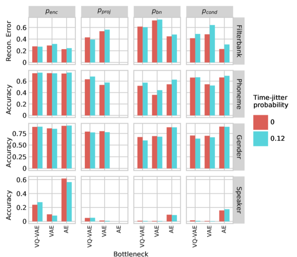
Figure 5: Impact of the time-jitter regularization on information captured by representations at different probe points.

We also analyzed information content at the four probe points for VQ-VAE, VAE, and simple dimensionality reduction AE bottleneck, shown in Figure 5. For all bottleneck mechanisms, the regularization limits the quality of filterbank reconstructions and increases the phoneme recognition accuracy in the constrained representation. However this benefit is smaller after neighboring timesteps are combined in the $p_{\text{cond}}$ probe point. Moreover, for VQ-VAE and VAE the regularization decreases gender prediction accuracy and makes the representation slightly less speaker-sensitive.

TABLE III: Effects of input representation and regularization on phoneme recognition accuracy on LibriSpeech, measured after 200k training steps. All models extract 256 tokens.

Input features	Token rate	Regularization	Accuracy
MFCC	25 Hz	None	52.5
MFCC	25 Hz	Regular dropout $p=0.1$	50.7
MFCC	25 Hz	Regular dropout $p=0.2$	49.1
MFCC	25 Hz	Per-time step dropout $p=0.2$	55.3
MFCC	25 Hz	Per-time step dropout $p=0.3$	55.7
MFCC	25 Hz	Per-time step dropout $p=0.4$	55.1
MFCC	25 Hz	Time-jitter $p=0.08$	56.2
MFCC	25 Hz	Time-jitter $p=0.12$	56.2
MFCC	25 Hz	Time-jitter $p=0.16$	56.1
MFCC	50 Hz	None	46.5
MFCC	50 Hz	Time-jitter $p=0.5$	56.1
log-mel spectrogram	25 Hz	None	50.1
log-mel spectrogram	25 Hz	Time-jitter $p=0.12$	53.6
raw waveform	30 Hz	None	37.6
raw waveform	30 Hz	Time-jitter $p=0.12$	48.1

IV-E2 Input representation

In this set of experiments we compared performance using different input representation: raw waveforms, log-mel spectrograms, or MFCCs. The raw waveform encoder used 9 strided convolutional layers, which resulted in token extraction frequency of 30 Hz. We then replaced the waveform with a customary ASR data pipeline: 80 log-mel filterbank features extracted every 10ms from 25ms-long windows and 13 MFCC features extracted from the mel-filterbank output, both augmented with their first and second temporal derivatives. Using two strided convolution layers in the encoder led to a 25 Hz token rate for these models.

The results are reported in the bottom of Table III. High-level features, especially MFCCs, perform better than waveforms, because by design they discard information about pitch and provide a degree of speaker invariance. Using such a reduced representation forces the encoder to transmit less information to the decoder, acting as an inductive bias toward a more speaker invariant latent encoding.

IV-E3 Output representation

We constructed an autoregressive decoder network that reconstructed filterbank features rather than raw waveform samples. Inspired by recent progress in text-to-speech systems, we implemented a Tacotron 2-like decoder [62] with a built-in information bottleneck on the autoregressive information flow, which was found to be critical in TTS applications. Similarly to Tacotron 2 the filterbank features were first processed by a small “pre-net”, we applied generous amounts of dropout and configured the decoder to predict up to 4 frames in parallel. However, these modifications yielded at best 42% phoneme recognition accuracy, significantly lower than the other architectures described in this paper. The model was however an order of magnitude faster to train.

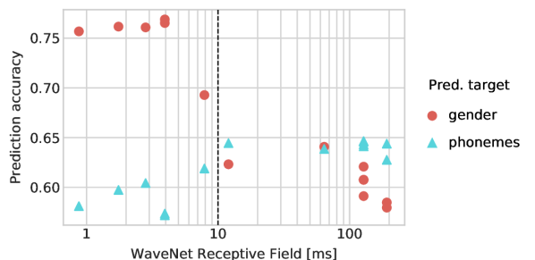
Figure 6: Impact of decoder WaveNet receptive field on the properties of the VQ-VAE conditioning signal. The representation is significantly more gender invariant when the receptive field is larger that 10ms. Frame-wise phoneme recognition accuracy peaks at about 125ms. The depth and width of the WaveNet have a secondary effect (cf. points with the same RF).

Finally, we analyzed the impact of the size of the decoding WaveNet on the representation extracted by the VQ-VAE. We have found that overall receptive field (RF) has a larger impact than the depth or width of the WaveNet. In particular, a large change in the properties of the latent representation happens when the decoder’s receptive field crosses than about 10ms. As shown in Figure 6, for smaller RFs, the conditioning signal contains more speaker information: gender prediction is close to 80%, while framewise phoneme prediction accuracy is only 55%. For larger RFs, gender prediction accuracy is about 60%, while phoneme prediction peaks near 65%. Finally, while the reconstruction log-likelihood improved with WaveNet depth up to 30 layers, the phoneme recognition accuracy plateaued with 20 layers. Since the WaveNet has the largest computational cost we decided to keep the 20 layer configuration.

IV-E4 Decoder speaker conditioning

The WaveNet decoder generates samples based on three sources of information: the previously emitted samples (via the autoregressive connection), global conditioning on speaker or other information which is stationary in time, and on the time-varying representation extracted from the encoder. We found that disabling global speaker conditioning reduces phoneme classification accuracy by 3 percentage points. This further corroborates our findings about disentanglement induced by the VQ-VAE bottleneck, which biases the model to discard information that is available in a more explicit form. Throughout our experiments we used a speaker-independent encoder. However, adapting the encoder to the speaker might further improve the results. In fact, [58] demonstrates improvements on the ZeroSpeech task using a speaker-adaptive approach.

IV-E5 Encoder hyperparameters

We experimented with tuning the number of encoder convolutional layers, as well as the number of filters, and the filter length. In general, performance improved with larger encoders, however we established that the encoder’s receptive field must be carefully controlled, with the best performing encoders seeing about 0.3 seconds of input signal for each generated token.

The effective receptive field can be controlled using two mechanisms: by carefully tuning the encoder architecture, or by designing an encoder with a wide receptive field, but limiting the duration of signal segments seen during training to the desired receptive field. In this way the model never learns to use its full capacity. When the model was trained on 2.5s long segments, an encoder with receptive field of 0.3s had framewise phoneme recognition accuracy of 56.5%, while and encoder with a receptive field of 0.8s scored only 54.3%. When trained on segments of 0.3s, both models performed similarly.

IV-E6 Bottleneck bit rate

The speech VQ-VAE encoder can be seen as encoding a signal using a very low bit rate. To achieve a predetermined target bit rate, one can control both the token rate (i.e., by controlling the degree of downsampling down in the encoder strided convolutions), and the number of tokens (or equivalently the number of bits) extracted at every step. We found that the token rate is a crucial parameter which must be chosen carefully, with the best results after 200k training steps obtained at 50 Hz (56.0% phoneme recognition accuracy ) and 25 Hz (56.3%). Accuracy drops abruptly at higher token rates (49.3% at 100 Hz), while lower rates miss very short phones (53% accuracy at 12.5 Hz).

In contrast to the number of tokens, the dimensionality of the VQ-VAE embedding has a secondary effect on representation quality. We found 64 to be a good setting, with much smaller dimensions deteriorating performance for models with a small number of tokens and higher dimensionalities negatively affecting performance for models with a large number of tokens.

For completeness, we observe that even for the model with the largest inventory of tokens, the overall encoder bitrate is low: 14 bits at 50 Hz = 700 bps, which is on par with the lowest bitrate of classical speech codecs [63].

IV-E7 Training corpus size

We experimented with training models on subsets of the LibriSpeech training set, varying the size from 4.6 hours (1%) to 460 hours (100%). Training on 4.6 hours of data, phoneme recognition accuracy peaked at 50.5% at 100k steps and then deteriorated. Training on 9 hours led to a peak accuracy of 52.5% at 180k sets. When the size of training set was increased past 23 hours the phoneme recognition reached 54% after around 900k steps. No further improvements were found by training on the full 460 hours of data. We did not observe any overfitting, and for best results trained models until reaching 900k steps with no early stopping. An interesting future area for research would be investigating methods to increase the model capacity to make better use of larger amounts of unlabeled data.

The influence of the size of the dataset is also visible in the ZeroSpeech Challenge results (Table II): VQ-VAE models obtained good performance on English (45 hours of training data) and French (24 hours), but performed poorly on Mandarin (2.5 hours). Moreover, on English and French we obtained the best results with models trained on monolingual data. On Mandarin slightly better results were obtained using a model trained jointly on data from all languages.

V Related Work

VAEs for sequential data were introduced in [49]. The model used LSTM encoder and decoder, while the latent representation was formed from the last hidden state of the encoder. The model proved useful for natural language processing tasks. However, it also demonstrated the problem of latent representation collapse: when a powerful autoregressive decoder is used simultaneously with a penalty on the latent encoding, such as the KL prior, the VAE has a tendency to ignore the prior and act as if it were a purely autoregressive sequence model. This issue can be mitigated by changing the weight of the KL term, and limiting the amount of information on the autoregressive path by using word dropout [49]. Latent collapse can also be avoided in deterministic autoencoders, such as [64], which coupled a convolutional encoder to a powerful autoregressive WaveNet decoder [18] to learn a latent representation of music audio consisting of isolated notes from a variety of instruments.

We empirically validate that conditioning the decoder on speaker information results in encodings which are more speaker invariant. Moyer et al. [54] give a rigorous proof that this approach produces representations that are invariant to the explicitly provided information and relate it to domain-adversarial training, another technique designed to enforce invariance to a known nuisance factor [65].

When applied to audio, the VQ-VAE uses the WaveNet decoder to free the latent representation from modeling information that is easily recoverable form the recent past [19]. It avoids the problem of posterior collapse by using a discrete latent code with a uniform prior which results in a constant KL penalty. We employ the same strategy to design the latent representation regularizer: rather than extending the cost function with a penalty term that can cause the latent space to collapse, we rely on random copies of the latent variables to prevent their co-adaptation and promote stability over time.

The randomized time-jitter regularization introduced in this paper is inspired by slow representations of data [48] and by dropout, which randomly removes during training neurons to prevent their co-adaptation [50]. It is also very similar to Zoneout [51] which relies on random time copies of selected neurons to regularize recurrent neural networks.

Several authors have recently proposed to model sequences with VAEs that use a hierarchy of variables. [66] explore a hierarchical latent space which separates sequence-dependent variables from those which are sequence-independent ones. Their model was shown to perform speaker conversion and to improve automatic speech recognititon (ASR) performance in the presence of domain mismatch. [67] introduce a stochastic latent variable model for sequential data which also yields disentangled representations and allows content swapping between generated sequences. These other approaches could possibly benefit from regularizing the latent representation to achieve further information disentanglement.

Acoustic unit discovery systems aim at transducing the acoustic signal into a sequence of interpretable units akin to phones. They often involve clustering of acoustic frames, MFCC or neural network bottleneck features, regularized using a probabilistic prior. DP-GMM [68] imposes a Dirichlet Process prior over a Gaussian Mixture Model. Extending it with an HMM temporal structure for sub-phonetic units leads to the DP-HMM and the HDP-HMM [69, 70, 71]. HMM-VAE proposes the use of a deep neural network instead of a GMM [72, 73]. These approaches enforce top-down constraints via HMM temporal smoothing and temporal modeling. Linguistic unit discovery models detect recurring speech patterns at a word-like level, finding commonly repeated segments with a constrained dynamic time warping [74].

In the segmental unsupervised speech recognition framework, neural autoencoders were used to embed variable length speech segments into a common vector space where they could be clustered into word types [75]. [76] replace the segmental autoencoder with a model that instead predicts a nearby speech segment and demonstrate that the representation shares many properties with word embeddings. Coupled with an unsupervised word segmentation algorithm and unsupervised mapping of word embeddings discovered on separate corpora [77] the approach yielded an ASR system trained on unpaired speech and text data [78].

Several entries to the ZeroSpeech 2017 challenge relied on neural networks for phonetic unit discovery. [61] trains an autoencoder on pairs of speech segments found using an unsupervised term discovery system [79]. [59] first clustered speech frames, then trained a neural network to predict the cluster IDs and used its hidden representation as features. [60] extended this scheme with features discovered by an autoencoder trained on MFCCs.

VI Conclusions

We applied sequence autoencoders to speech modeling and compared different information bottlenecks, including VAEs and VQ-VAEs. We carefully evaluated the induced latent representation using interpretability criteria as well as the ability to discriminate between similar speech sounds. The comparison of bottlenecks revealed that discrete representations obtained using VQ-VAE preserved the most phonetic information while also being the most speaker-invariant. The extracted representation allowed for accurate mapping of the extracted symbols into phonemes and obtained competitive performance on the ZeroSpeech 2017 acoustic unit discovery task. A similar combination of VQ-VAE encoder and WaveNet decoder by Cho et al. had the best acoustic unit discovery performance in ZeroSpeech 2019 [80].

We established that an information bottleneck is required for the model to learn a representation that separates content from speaker characteristics. Furthermore, we observe that the latent collapse problem induced by bottlenecks which are too strong can be avoided by making the bottleneck strength a model hyperparameter, either removing it completely (as in the VQ-VAE), or by using the free-information VAE objective.

To further improve representation quality, we introduced a time-jitter regularization scheme which limits the capacity of the latent code yet does not result in a collapse of the latent space. We hope that this can similarly improve performance of latent variable models used with auto-regressive decoders in other problem domains.

Both the VAE and VQ-VAE constrain the information bandwidth of the latent representation. However, the VQ-VAE uses a quantization mechanism, which deterministically forces the encoding to be equal to a prototype, while the VAE limits the amount of information by injecting noise. In our study, the VQ-VAE resulted in better information separation than the VAE. However, further experiments are needed to fully understand this effect. In particular, is this a consequence of the quantization, or of the deterministic operation?

We also observe that while the VQ-VAE produces a discrete representation, for best results it uses a token set so large that it is impractical to assign a separate meaning to each one. In particular, in our ZeroSpeech experiments we used the dense embedding representation of each token, which provided a more nuanced token similarity measure than simply using the token identity. Perhaps a more structured latent representation is needed, in which a small set of units can be modulated in a continuous fashion.

Extensive hyperparameter evaluation indicated that optimizing the receptive field sizes of the encoder and decoder networks is important for good model performance. A multi-scale modeling approach could furthermore separate the prosodic information. Our autoencoding approach could also be combined with penalties that are more specialized to speech processing. Introducing a HMM prior as in [73] could promote a latent representation which better mimics the temporal phonetic structure of speech.

Jan Chorowski is an Associate Professor at Faculty of Mathematics and Computer Science at the University of Wrocław. He received his M.Sc. degree in electrical engineering from the Wrocław University of Technology, Poland and EE PhD from the University of Louisville, Kentucky in 2012. He has worked with several research teams, including Google Brain, Microsoft Research and Yoshua Bengio’s lab at the University of Montreal. His research interests are applications of neural networks to problems which are intuitive for humans but difficult for machines, such as speech and natural language processing.

Ron J. Weiss is a software engineer at Google where he has worked on content-based audio analysis, recommender systems for music, noise robust speech recognition, speech translation, and speech synthesis. Ron completed his Ph.D. in electrical engineering from Columbia University in 2009 where he worked in the Laboratory for the Recognition of Speech and Audio. From 2009 to 2010 he was a postdoctoral researcher in the Music and Audio Research Laboratory at New York University.

Samy Bengio (PhD in computer science, University of Montreal, 1993) is a research scientist at Google since 2007. He currently leads a group of research scientists in the Google Brain team, conducting research in many areas of machine learning such as deep architectures, representation learning, sequence processing, speech recognition, image understanding, large-scale problems, adversarial settings, etc. He is the general chair for Neural Information Processing Systems (NeurIPS) 2018, the main conference venue for machine learning, was the program chair for NeurIPS in 2017, is action editor of the Journal of Machine Learning Research and on the editorial board of the Machine Learning Journal, was program chair of the International Conference on Learning Representations (ICLR 2015, 2016), general chair of BayLearn (2012-2015) and the Workshops on Machine Learning for Multimodal Interactions (MLMI’2004-2006), as well as the IEEE Workshop on Neural Networks for Signal Processing (NNSP’2002), and on the program committee of several international conferences such as NeurIPS, ICML, ICLR, ECML and IJCAI.

Aäron van den Oord is a research scientist at DeepMind, London. Aäron completed his PhD at the University of Ghent, Belgium in 2015. He has worked on unsupervised representation learning, music recommendation, generative modeling with autoregressive networks and various applications of generative models such text-to-speech synthesis and data compression.

References

- [1] G. E. Hinton and R. R. Salakhutdinov, “Reducing the dimensionality of data with neural networks,” Science, vol. 313, no. 5786, 2006.
- [2] P. Vincent, H. Larochelle, Y. Bengio, and P.-A. Manzagol, “Extracting and composing robust features with denoising autoencoders,” in Proc. International Conference on Machine Learning, 2008.
- [3] A. Krizhevsky, I. Sutskever, and G. E. Hinton, “Imagenet classification with deep convolutional neural networks,” in Advances in Neural Information Processing Systems, 2012, pp. 1097–1105.
- [4] C. Szegedy, W. Liu, Y. Jia, P. Sermanet, S. Reed, D. Anguelov, D. Erhan, V. Vanhoucke, and A. Rabinovich, “Going deeper with convolutions,” in Proc. IEEE Conference on Computer Vision and Pattern Recognition, 2015.
- [5] D. Bahdanau, K. Cho, and Y. Bengio, “Neural machine translation by jointly learning to align and translate,” in Proc. International Conference on Learning Representations, 2015.
- [6] Y. Wu, M. Schuster, Z. Chen, Q. V. Le, M. Norouzi, W. Macherey, M. Krikun, Y. Cao, Q. Gao, K. Macherey, and et al, “Google’s neural machine translation system: Bridging the gap between human and machine translation,” arXiv preprint arXiv:1609.08144, 2016.
- [7] A. Graves, A.-r. Mohamed, and G. Hinton, “Speech recognition with deep recurrent neural networks,” in Proc. International Conference on Acoustics, Speech and Signal Processing (ICASSP), 2013, pp. 6645–6649.
- [8] C.-C.Chiu, T. N. Sainath, Y. Wu, R. Prabhavalkar, P. Nguyen, Z. Chen, A. Kannan, R. J. Weiss, K. Rao, K. Gonina, N. Jaitly, B. Li, J. Chorowski, and M. Bacchiani, “State-of-the-art speech recognition with sequence-to-sequence models,” in Proc. International Conference on Acoustics, Speech and Signal Processing (ICASSP), 2018.
- [9] W. Wang, N. Yang, F. Wei, B. Chang, and M. Zhou, “Gated self-matching networks for reading comprehension and question answering,” in Proc. 55th Annual Meeting of the Association for Computational Linguistics (Volume 1: Long Papers), vol. 1, 2017, pp. 189–198.
- [10] A. W. Yu, D. Dohan, M.-T. Luong, R. Zhao, K. Chen, M. Norouzi, and Q. V. Le, “QANet: Combining local convolution with global self-attention for reading comprehension,” in Proc. International Conference on Learning Representations, 2018.
- [11] M. D. Zeiler and R. Fergus, “Visualizing and understanding convolutional networks,” in European Conference on Computer Vision, 2014.
- [12] M. Sundararajan, A. Taly, and Q. Yan, “Axiomatic attribution for deep networks,” in Proc. International Conference on Machine Learning, 2017.
- [13] T. Nagamine and N. Mesgarani, “Understanding the representation and computation of multilayer perceptrons: A case study in speech recognition,” in Proc. International Conference on Machine Learning, 2017.
- [14] J. Chorowski, R. J. Weiss, R. A. Saurous, and S. Bengio, “On using backpropagation for speech texture generation and voice conversion,” in Proc. International Conference on Acoustics, Speech and Signal Processing (ICASSP), Apr. 2018.
- [15] P. Swietojanski, A. Ghoshal, and S. Renals, “Unsupervised cross-lingual knowledge transfer in DNN-based LVCSR,” in Proc. Spoken Language Technology Workshop (SLT), 2012, pp. 246–251.
- [16] S. Thomas, M. L. Seltzer, K. Church, and H. Hermansky, “Deep neural network features and semi-supervised training for low resource speech recognition,” in Proc. International Conference on Acoustics, Speech and Signal Processing (ICASSP), 2013, pp. 6704–6708.
- [17] V. Panayotov, G. Chen, D. Povey, and S. Khudanpur, “LibriSpeech: an ASR corpus based on public domain audio books,” in Proc. International Conference on Acoustics, Speech and Signal Processing (ICASSP), 2015.
- [18] A. van den Oord, S. Dieleman, H. Zen, K. Simonyan, O. Vinyals, A. Graves, N. Kalchbrenner, A. Senior, and K. Kavukcuoglu, “WaveNet: A generative model for raw audio,” arXiv preprint arXiv:1609.03499, 2016.
- [19] A. van den Oord, O. Vinyals, and K. Kavukcuoglu, “Neural discrete representation learning,” in Advances in Neural Information Processing Systems, 2017, pp. 6309–6318.
- [20] E. Dunbar, X. N. Cao, J. Benjumea, J. Karadayi, M. Bernard, L. Besacier, X. Anguera, and E. Dupoux, “The zero resource speech challenge 2017,” in Proc. Automatic Speech Recognition and Understanding Workshop (ASRU), 2017.
- [21] D. E. Rumelhart, G. E. Hinton, and R. J. Williams, “Learning representations by back-propagating errors,” Nature, vol. 323, no. 6088, 1986.
- [22] H. Lee, C. Ekanadham, and A. Ng, “Sparse deep belief net model for visual area V2,” in Advances in Neural Information Processing Systems, 2008.
- [23] S. Dieleman and B. Schrauwen, “End-to-end learning for music audio,” in Proc. International Conference on Acoustics, Speech and Signal Processing (ICASSP), 2014, pp. 6964–6968.
- [24] N. Jaitly and G. Hinton, “Learning a better representation of speech soundwaves using restricted Boltzmann machines,” in Proc. International Conference on Acoustics, Speech and Signal Processing (ICASSP), 2011.
- [25] Z. Tüske, P. Golik, R. Schlüter, and H. Ney, “Acoustic modeling with deep neural networks using raw time signal for LVCSR,” in Proc. Interspeech, 2014.
- [26] D. Palaz, M. Magima Doss, and R. Collobert, “Analysis of CNN-based speech recognition system using raw speech as input,” in Proc. Interspeech, 2015.
- [27] T. N. Sainath, R. J. Weiss, A. Senior, K. W. Wilson, and O. Vinyals, “Learning the speech front-end with raw waveform CLDNNs,” in Proc. Interspeech, 2015.
- [28] J. Deng, W. Dong, R. Socher, L.-J. Li, K. Li, and L. Fei-Fei, “ImageNet: A Large-Scale Hierarchical Image Database,” in Proc. IEEE Conference on Computer Vision and Pattern Recognition, 2009.
- [29] J. Yosinski, J. Clune, Y. Bengio, and H. Lipson, “How transferable are features in deep neural networks?” in Advances in Neural Information Processing Systems, 2014, pp. 3320–3328.
- [30] K. Veselỳ, M. Karafiát, F. Grézl, M. Janda, and E. Egorova, “The language-independent bottleneck features,” in Proc. Spoken Language Technology Workshop (SLT), 2012, pp. 336–341.
- [31] D. Yu and M. L. Seltzer, “Improved bottleneck features using pretrained deep neural networks,” in Proc. Interspeech, 2011.
- [32] B. McCann, J. Bradbury, C. Xiong, and R. Socher, “Learned in translation: Contextualized word vectors,” in Advances in Neural Information Processing Systems, 2017, pp. 6294–6305.
- [33] S. R. Bowman, G. Angeli, C. Potts, and C. Manning, “A large annotated corpus for learning natural language inference,” in Proc. Conference on Empirical Methods in Natural Language Processing, 2015.
- [34] A. Conneau, D. Kiela, H. Schwenk, L. Barrault, and A. Bordes, “Supervised learning of universal sentence representations from natural language inference data,” in Proc. Conference on Empirical Methods in Natural Language Processing (EMNLP), September 2017, pp. 670–680.
- [35] C. M. Bishop, “Continuous latent variables,” in Pattern Recognition and Machine Learning. Springer, 2006, ch. 12.
- [36] D. D. Lee and H. S. Seung, “Learning the parts of objects by non-negative matrix factorization,” Nature, vol. 401, no. 6755, p. 788, 1999.
- [37] B. A. Olshausen and D. J. Field, “Emergence of simple-cell receptive field properties by learning a sparse code for natural images,” Nature, vol. 381, no. 6583, p. 607, 1996.
- [38] D. P. Kingma and M. Welling, “Auto-encoding variational bayes,” in Proc. International Conference on Learning Representations, 2014.
- [39] I. Higgins, L. Matthey, A. Pal, C. Burgess, X. Glorot, M. Botvinick, S. Mohamed, and A. Lerchner, “Beta-VAE: Learning basic visual concepts with a constrained variational framework,” in Proc. International Conference on Learning Representations, 2017.
- [40] A. A. Alemi, I. Fischer, J. V. Dillon, and K. Murphy, “Deep variational information bottleneck,” in Proc. International Conference on Learning Representations, 2017.
- [41] D. P. Kingma, T. Salimans, R. Jozefowicz, X. Chen, I. Sutskever, and M. Welling, “Improved variational inference with inverse autoregressive flow,” in Advances in Neural Information Processing Systems, 2016.
- [42] Y. Bengio, N. Léonard, and A. Courville, “Estimating or propagating gradients through stochastic neurons for conditional computation,” arXiv preprint arXiv:1308.3432, 2013.
- [43] D. Jurafsky and J. H. Martin, Speech and Language Processing (2nd Edition). Upper Saddle River, NJ, USA: Prentice-Hall, Inc., 2009.
- [44] Y. N. Dauphin, A. Fan, M. Auli, and D. Grangier, “Language modeling with gated convolutional networks,” in Proc. International Conference on Machine Learning, 2017.
- [45] S. Bai, J. Z. Kolter, and V. Koltun, “An empirical evaluation of generic convolutional and recurrent networks for sequence modeling,” arXiv preprint arXiv:1803.01271, 2018.
- [46] W.-N. Hsu, Y. Zhang, R. J. Weiss, H. Zen, Y. Wu, Y. Wang, Y. Cao, Y. Jia, Z. Chen, J. Shen, P. Nguyen, and R. Pang, “Hierarchical generative modeling for controllable speech synthesis,” in Proc. International Conference on Learning Representations, 2019.
- [47] I. Gulrajani, K. Kumar, F. Ahmed, A. A. Taïga, F. Visin, D. Vázquez, and A. Courville, “PixelVAE: A latent variable model for natural images,” in Proc. International Conference on Learning Representations, 2017.
- [48] L. Wiskott and T. J. Sejnowski, “Slow feature analysis: Unsupervised learning of invariances,” Neural Computation, vol. 14, no. 4, 2002.
- [49] S. R. Bowman, L. Vilnis, O. Vinyals, A. M. Dai, R. Jozefowicz, and S. Bengio, “Generating sentences from a continuous space,” in SIGNLL Conference on Computational Natural Language Learning, 2016.
- [50] N. Srivastava, G. Hinton, A. Krizhevsky, I. Sutskever, and R. Salakhutdinov, “Dropout: A simple way to prevent neural networks from overfitting,” Journal of Machine Learning Research, vol. 15, no. 1, 2014.
- [51] D. Krueger, T. Maharaj, J. Kramár, M. Pezeshki, N. Ballas, N. R. Ke, A. Goyal, Y. Bengio, A. Courville, and C. Pal, “Zoneout: Regularizing RNNs by randomly preserving hidden activations,” in Proc. International Conference on Learning Representations, 2017.
- [52] D. P. Kingma and J. Ba, “Adam: A method for stochastic optimization,” in Proc. International Conference on Learning Representations, 2015.
- [53] B. T. Polyak and A. B. Juditsky, “Acceleration of stochastic approximation by averaging,” SIAM Journal on Control and Optimization, vol. 30, no. 4, pp. 838–855, 1992.
- [54] D. Moyer, S. Gao, R. Brekelmans, A. Galstyan, and G. Ver Steeg, “Invariant Representations without Adversarial Training,” in Advances in Neural Information Processing Systems 31, 2018, pp. 9084–9093.
- [55] D. Povey, A. Ghoshal, G. Boulianne, L. Burget, O. Glembek, N. Goel, M. Hannemann, P. Motlicek, Y. Qian, P. Schwarz, J. Silovsky, G. Stemmer, and K. Vesely, “The Kaldi speech recognition toolkit,” in Proc. Automatic Speech Recognition and Understanding Workshop (ASRU), 2011.
- [56] T. Schatz, V. Peddinti, F. Bach, A. Jansen, H. Hermansky, and E. Dupoux, “Evaluating speech features with the minimal-pair ABX task: Analysis of the classical MFC/PLP pipeline,” in Proc. Interspeech, 2013, pp. 1–5.
- [57] T. Schatz, V. Peddinti, X.-N. Cao, F. Bach, H. Hermansky, and E. Dupoux, “Evaluating speech features with the minimal-pair ABX task (ii): Resistance to noise,” in Proc. Interspeech, 2014.
- [58] M. Heck, S. Sakti, and S. Nakamura, “Unsupervised linear discriminant analysis for supporting DPGMM clustering in the zero resource scenario,” Procedia Computer Science, vol. 81, pp. 73–79, 2016.
- [59] H. Chen, C.-C. Leung, L. Xie, B. Ma, and H. Li, “Multilingual bottle-neck feature learning from untranscribed speech,” in Proc. Automatic Speech Recognition and Understanding Workshop (ASRU), 2017.
- [60] T. Ansari, R. Kumar, S. Singh, and S. Ganapathy, “Deep learning methods for unsupervised acoustic modeling—leap submission to zerospeech challenge 2017,” in Proc. Automatic Speech Recognition and Understanding Workshop (ASRU), 2017, pp. 754–761.
- [61] Y. Yuan, C. C. Leung, L. Xie, H. Chen, B. Ma, and H. Li, “Extracting bottleneck features and word-like pairs from untranscribed speech for feature representation,” in Proc. Automatic Speech Recognition and Understanding Workshop (ASRU), Dec 2017, pp. 734–739.
- [62] J. Shen, R. Pang, R. J. Weiss, M. Schuster, N. Jaitly, Z. Yang, Z. Chen, Y. Zhang, Y. Wang, R. J. Skerry-Ryan, R. A. Saurous, Y. Agiomyrgiannakis, and Y. Wu, “Natural TTS synthesis by conditioning WaveNet on mel spectrogram predictions,” in Proc. International Conference on Acoustics, Speech and Signal Processing (ICASSP), 2018.
- [63] X. Wang and C.-C. J. Kuo, “An 800 bps VQ-based LPC voice coder,” Journal of the Acoustical Society of America, vol. 103, no. 5, 1998.
- [64] J. Engel, C. Resnick, A. Roberts, S. Dieleman, M. Norouzi, D. Eck, and K. Simonyan, “Neural audio synthesis of musical notes with wavenet autoencoders,” in Proc. International Conference on Machine Learning, 2017, pp. 1068–1077.
- [65] Y. Ganin, E. Ustinova, H. Ajakan, P. Germain, H. Larochelle, F. Laviolette, M. Marchand, and V. Lempitsky, “Domain-Adversarial Training of Neural Networks,” Journal of Machine Learning Research, vol. 17, no. 59, pp. 1–35, 2016.
- [66] W.-N. Hsu, Y. Zhang, and J. Glass, “Unsupervised learning of disentangled and interpretable representations from sequential data,” in Advances in Neural Information Processing Systems, 2017, pp. 1876–1887.
- [67] Y. Li and S. Mandt, “Disentangled sequential autoencoder,” in Proc. International Conference on Machine Learning, 2018.
- [68] H. Chen, C.-C. Leung, L. Xie, B. Ma, and H. Li, “Parallel Inference of Dirichlet Process Gaussian Mixture Models for Unsupervised Acoustic Modeling: A Feasibility Study,” in Proc. Interspeech, 2015.
- [69] C.-y. Lee and J. Glass, “A Nonparametric Bayesian Approach to Acoustic Model Discovery,” in Proc. 50th Annual Meeting of the Association for Computational Linguistics (Volume 1: Long Papers), Jul. 2012, pp. 40–49.
- [70] L. Ondel, L. Burget, and J. Černocký, “Variational Inference for Acoustic Unit Discovery,” Procedia Computer Science, vol. 81, Jan. 2016.
- [71] R. Marxer and H. Purwins, “Unsupervised Incremental Online Learning and Prediction of Musical Audio Signals,” IEEE/ACM Transactions on Audio, Speech, and Language Processing, vol. 24, no. 5, May 2016.
- [72] J. Ebbers, J. Heymann, L. Drude, T. Glarner, R. Haeb-Umbach, and B. Raj, “Hidden Markov Model Variational Autoencoder for Acoustic Unit Discovery,” in Proc. Interspeech, Aug. 2017, pp. 488–492.
- [73] T. Glarner, P. Hanebrink, J. Ebbers, and R. Haeb-Umbach, “Full Bayesian Hidden Markov Model Variational Autoencoder for Acoustic Unit Discovery,” in Proc. Interspeech, Sep. 2018, pp. 2688–2692.
- [74] A. S. Park and J. R. Glass, “Unsupervised Pattern Discovery in Speech,” IEEE Transactions on Audio, Speech, and Language Processing, vol. 16, no. 1, pp. 186–197, Jan. 2008.
- [75] H. Kamper, A. Jansen, and S. Goldwater, “A segmental framework for fully-unsupervised large-vocabulary speech recognition,” Computer Speech & Language, vol. 46, pp. 154–174, 2017.
- [76] Y.-A. Chung and J. Glass, “Learning word embeddings from speech,” arXiv preprint arXiv:1711.01515, 2017.
- [77] G. Lample, A. Conneau, L. Denoyer, and M. Ranzato, “Unsupervised Machine Translation Using Monolingual Corpora Only,” in Proc. International Conference on Learning Representations, 2018.
- [78] Y.-A. Chung, W.-H. Weng, S. Tong, and J. Glass, “Unsupervised cross-modal alignment of speech and text embedding spaces,” Advances in Neural Information Processing Systems, 2018.
- [79] A. Jansen and B. Van Durme, “Efficient spoken term discovery using randomized algorithms,” in Proc. Automatic Speech Recognition and Understanding Workshop (ASRU), 2011, pp. 401–406.
- [80] E. Dunbar, R. Algayres, J. Karadayi, M. Bernard, J. Benjumea, X.-N. Cao, L. Miskic, C. Dugrain, L. Ondel, A. W. Black, L. Besacier, S. Sakti, and E. Dupoux, “The Zero Resource Speech Challenge 2019: TTS without T,” arXiv preprint arXiv:1904.11469, 2019, accepted to Interspeech 2019.