Metric Spaces with Expensive Distances

Abstract

In algorithms for finite metric spaces, it is common to assume that the distance between two points can be computed in constant time, and complexity bounds are expressed only in terms of the number of points of the metric space. We introduce a different model where we assume that the computation of a single distance is an expensive operation and consequently, the goal is to minimize the number of such distance queries. This model is motivated by metric spaces that appear in the context of topological data analysis.

We consider two standard operations on metric spaces, namely the construction of a $1+\varepsilon$-spanner and the computation of an approximate nearest neighbor for a given query point. In both cases, we partially explore the metric space through distance queries and infer lower and upper bounds for yet unexplored distances through triangle inequality. For spanners, we evaluate several exploration strategies through extensive experimental evaluation. For approximate nearest neighbors, we prove that our strategy returns an approximate nearest neighbor after a logarithmic number of distance queries.

Keywords metric spaces, doubling dimension, spanners, approximate nearest neighbor

1 Introduction

Given a set $P:=\{p_{1},\ldots,p_{n}\}$ of $n$ points in a metric space $(\mathcal{M},\delta)$, consider the following standard operations:

Approximate Nearest Neighbor

Given $\varepsilon>0$ and a point $q\in\mathcal{M}$, find $p_{i}\in P$ such that, for all $j=1,\ldots,n$,

$$\delta(q,p_{i})\leq(1+\varepsilon)\delta(q,p_{j})$$

Spanner

Given $\varepsilon>0$, compute a weighted graph $G$ with vertices in $P$ such that for any $u,v\in P$, the shortest path distance between $u$ and $v$ is at most $(1+\varepsilon)\delta(u,v)$.

The performance of algorithms for these problems depends on the number of points, the dimension of the metric space, and the cost $C_{\delta}$ of computing a distance in the metric space. It is a common assumption to assume $C_{\delta}$ to be a constant; There are good reasons for that: the most common case of a metric space is $\mathcal{M}=\mathbb{R}^{d}$ with $d$ some constant, in which case $C_{\delta}$ can be evaluated in $O(d)=O(1)$ time. Even if $d$ is considered non-constant, it can always be assumed that $d\leq n$, hence $C_{\delta}$ is at most $O(n)$. Another typical assumption is that all pairwise distances are part of the input in which case $C_{\delta}$ is $O(1)$.

However, we argue that in some situations, distance computations in $\mathcal{M}$ can be costly and $C_{\delta}$ might be incomparable with $n$. Our motivation comes from topological summaries such as persistence diagrams Edelsbrunner et al. (2002) or Reeb graphs Biasotti et al. (2008), which are of interest in the field of topological data analysis. A persistence diagram is a point set in $\mathbb{R}^{2}$, and the distance between two diagrams is determined by a min-cost matching between the point sets. If the diagrams have $N$ points, computing this matching requires polynomial time in $N$, and $N$ might well be larger than $n$, the number of diagrams considered (Cohen-Steiner et al. (2007)). For the case of Reeb graphs, the situation is even worse: while several metrics on Reeb graphs have been proposed (Bauer et al. (2014), De Silva et al. (2016), Di Fabio and Landi (2016)), not even an constant-factor approximation algorithm is known that runs in polynomial time in the size of the graphs. Another instance is a collection of high-resolution images endowed with the Wasserstein (or Earth Movers) metric (Rubner et al. (2000)).

In such situations with expensive distance computations, it makes sense to study a different cost model, where only the number of distance computations is taken into account. For instance, that means that quadratic time operations in terms of $n$ are not counted towards the time complexity, as long as these operations do not query any distance in $\mathcal{M}$. We also ignore the space complexity in our model.

We will restrict to the case of doubling spaces, that is, the doubling dimension of $\mathcal{M}$ is bounded by a constant. In that situation, standard constructions from computational geometry provide partial answers: Using net-trees Har-Peled and Mendel (2006), we can construct a $\varepsilon$-well-separated pair decomposition (WSPD) Callahan and Kosaraju (1995a) using $O(n\log n)$ distance queries; a WSPD in turn yields an $\varepsilon$-spanner immediately. Net-trees can also be used to compute approximate nearest neighbors performing $O(\log n)$ distance computations per query point. Krauthgamer and Lee Krauthgamer and Lee (2005) investigated black box model, and proved that ANN search for $\varepsilon<2/5$ can be done efficiently (i.e., in polylogarithmic time, with polynomial preprocessing and space) if and only if the dimension is $O(\log\log n)$; their bounds count the number of distance computations. However, for our relaxed cost model, we pose the question whether simpler constructions achieve comparable, or even fewer distance computations.

We also propose a slight variant of our model: we assume that we also have access to an (efficient) $2$-approximation algorithm for the distance queries. Queries to this approximation algorithm are not counted in the model, hence we can assume that for each pair of points $(u,v)$, we know a number $A_{u,v}$ with $\delta(u,v)\leq A_{u,v}\leq 2\delta(u,v)$. This induces an approximate ordering of all distances in the metric space, and it is plausible to assume that such an ordering will simplify algorithmic tasks on metric spaces, at least in practice.

Contributions. We propose simple algorithms for spanner construction and approximate nearest neighbor search and evaluate them theoretically and experimentally in the defined cost model.

Our algorithms are based on the following simple idea: since distance computations are expensive and should be avoided, we try to obtain maximal information out of the distances that have been computed so far. This information consists of lower and upper bounds for unknown distances, obtained from known distances by triangle inequality (see Figure 1). We remark that updating these bounds involves $\Omega(n^{2})$ arithmetic operations whenever a new distance has been computed, turning the method useless in the standard computational model.

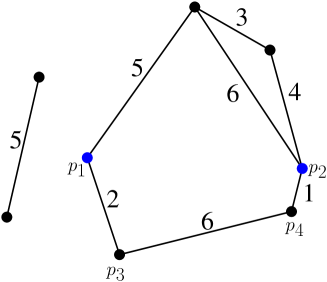
Figure 1: The compute distances are shown as edges in a graph. Note that the exact distance of $p_{1}$ and $p_{2}$ is unknown. The shortest path from $p_{1}$ to $p_{2}$ has length $9$, which clearly constitutes an upper bound on the distance by triangle inequality. However, we can also infer that $\delta(p_{1},p_{2})\geq 3$: otherwise, the path from $p_{3}$ to $p_{4}$ via $p_{1}$ and $p_{2}$ would be shorter than the edge $(p_{3},p_{4})$, again contradicting triangle inequality.

We propose several heuristics of how to explore the metric space to obtain accurate lower and upper bounds with a small number of distance computation. Once the ratio of upper and lower bound is at most $(1+\varepsilon)$ for each point pair, the set of all computed distances forms the spanner. The experimentally most successful exploration strategy that we found is to repeatedly query the distance of a pair with the worst ratio of upper and lower bound. We call the obtained spanner the blind greedy spanner, as opposed to the well-known greedy spanner that precomputes all pairwise distances and only maintains upper bounds (Althöfer et al. (1993)). Remarkably, we were not able to improve the quality when knowing initial $2$-approximations of all point pairs. We also compare with a spanner construction based on WSPD. Our simple algorithms tend to give much smaller spanners on the tested example. Nevertheless, we leave the question open whether our construction yields a spanner of asymptotically linear size.

For approximate nearest neighbor, we devise a simple randomized incremental algorithm and show that the number of distance queries to find an approximate nearest neighbor is $O(\log n)$ in expectation. Our proof is based on the well-known observation that the nearest neighbor changes $O(\log n)$ times in expectation when traversing the sequence of points, combined with a packing argument certifying that only a constant number of distances needs to be computed in-between two minima. We also experimentally evaluate our approach and observe that the approach follows roughly the theoretical prediction.

2 Background and Definitions

Doubling dimension. A metric space is called doubling with doubling constant $k$, if every ball of radius $r$ can be covered by at most $k$ balls of radius $r/2$, and $k$ is the smallest number having that property. The doubling dimension of a doubling space is defined as $\log k$ (since we usually ignore multiplicative constants, the base of the logarithm is not really important; however, we always use $\log$ to denote the logarithm with base 2). It is easy to see that a subspace of a space with doubling dimension $d$ is always doubling and has the doubling dimension $O(d)$ (but not necessarily $d$).

We shall need the following lemma, which is just a reformulation of the well-known packing lemma for doubling spaces (see Smid (2009), Sect. 2.2).

Lemma 1.

Let $(\mathcal{M},\delta)$ be a metric space of doubling dimension $d$, and let $P$ be a subset of a ball $B(x,R)$ in $\mathcal{M}$ such that the distance between any two distinct points of $P$ is at least $r$. Then

$$|P|\leq\left(\frac{4R}{r}\right)^{d}$$

Proof.

We can cover $B(x,R)$ with $2^{d}$ ball of radius $R/2$, each of these balls we can cover with $2^{d}$ balls of radius $R/4$, etc. Repeating this process $m:=\lceil\log\frac{R}{r/2}\rceil$ times, we cover $B(x,R)$ with $2^{md}$ balls of radius at most $r/2$. Since a ball of radius $r/2$ can contain at most one point from $P$,

$$|P|\leq 2^{md}=2^{\lceil\log\frac{R}{r/2}\rceil d}\leq 2^{(1+\log\frac{R}{r/2})d}=\left(\frac{4R}{r}\right)^{d}.\qed$$

In the following, we will assume throughout that every considered metric space has a constant doubling dimension.

Well-separated pair decomposition. Given $t>1$, two disjoint subsets $A,B$ of a metric space $(\mathcal{M},\delta)$ are called $t$-well-separated, if

$$\forall a\in A\,\,\forall b\in B\,\,\delta(a,b)\geq t\max(\mathrm{diam}(A),\mathrm{diam}(B))$$

A well-separated pair decomposition (WSPD) is a set of unordered pairs of sets $\{\{A_{1},B_{1}\},\dots,\{A_{s},B_{s}\}\}$ such that each pair $\{A_{i},B_{i}\}$ is $s$-well-separated, and for every unordered pair $\{a,b\}$ of distinct points of $\mathcal{M}$ there exists a unique $j$ such that $a\in A_{j}$ and $b\in B_{j}$. The notion of WSPD was introduced by Callahan and Kosaraju Callahan and Kosaraju (1995b) for Euclidean spaces. Har-Peled and Mendel Har-Peled and Mendel (2006) introduced the notion of net-trees and generalized the results of Callahan and Kosaraju (1995b) for WSPD, proving the following:

1. A net-tree for a metric space with $n$ points can be constructed in $2^{O(\mbox{dim})}n\log n$ expected time.

2. If $\{\{A_{1},B_{1}\},\dots,\{A_{s},B_{s}\}\}$ is an $\varepsilon/16$-WSPD on $\mathcal{M}$, and $a_{i}\in A_{i},b_{i}\in B_{i}$ for $i=1\dots s$ are chosen arbitrarily, then we get an $\varepsilon$-spanner by taking $s$ edges $(a_{i},b_{i})$.

3. For $\varepsilon\in(0,1]$, an $\varepsilon$-WSPD of size $n\varepsilon^{-O({\dim})}$ can be constructed in $2^{O({\dim})}n\log n+n\varepsilon^{-O({\dim})}$ expected time. The algorithm uses the net-tree structure.

The algorithm of constructing a net-tree is complicated and not easy to implement. Beygelzimer et al. Beygelzimer et al. (2006) introduced the notion of a cover tree, which is a simpler data structure than net-trees. We mention in passing that cover trees can also be used for building a spanner (this can be proven with the same methods), and we use cover trees for building WSPD spanners in one of our implementations.

3 Algorithms for spanner construction

Spanners and known constructions. Let $(\mathcal{M},\delta)$ be a finite metric space with $n$ points. One way to encode the metric space is a complete weighted graph on $\mathcal{M}$, where the weights correspond to the distances of the points. A subgraph $G$ of this graph is called a $(1+\varepsilon)$-spanner for $(\mathcal{M},\delta)$ if for any pair of points $(u,v)$, the shortest path distance $d_{uv}$ of $u$ and $v$ in $G$ satisfies $d_{u,v}\leq(1+\varepsilon)\delta(u,v)$. In other words, the shortest path metric of $G$ is a good approximation of the actual distance for every pair of points. Clearly, it is a necessary condition that $G$ is connected, hence every spanner must have at least $n-1$ edges.

The greedy spanner(Althöfer et al. (1993)) is a simple algorithm to compute linear-sized spanners:

function GreedySpanner($P,\varepsilon$)

     $E\leftarrow\emptyset$

     Sort all pairwise distances of points in $P$

     for all pairs $(p_{i},p_{j})$ in increasing order do

         $d_{ij}\leftarrow$ Shortest path distance in $(P,E)$

         if $d_{ij}>(1+\varepsilon)\delta(p_{i},p_{j})$ then

              Add weighted edge $(p_{i},p_{j},v)$ to $E$               return $(P,E)$

The greedy spanner is guaranteed (Althöfer et al. (1993)) to return a spanner of size $O(n)$ (for constant doubling dimension and fixed $\varepsilon>0$); in experimental study Farshi and Gudmundsson (2009) it was also shown to return the sparsest graph. However, it clearly has to compute all $\binom{n}{2}$ pairwise distances in the sorting step; this means that in our cost model, the greedy spanner has the worst possible performance.

On the other hand, spanner constructions based on WSPD only compute $O(n\log n+n\varepsilon^{-d})$ distances to construct an $(1+\varepsilon)$-spanner in doubling dimension $d$. The spanner size is $O(n\varepsilon^{-d})$. Assuming $\varepsilon$ and $d$ again as constants, this construction yields a $O(n)$-size spanner using only $O(n\log n)$ distance computations. However, the algorithm is significantly more involved.

Blind spanners. We introduce a new framework for constructing spanners which we call blind spanners: the idea is to maintain, for every pair of points $(p_{i},p_{j})$, a lower bound $a_{ij}$ and an upper bound $b_{ij}$ for $\delta(p_{i},p_{j})$, initially set to $[0,\infty)$. While there exists some pair for which $\frac{b_{ij}}{a_{ij}}>(1+\varepsilon)$, we pick one of them, compute its distance and update the lower and upper bounds of all pairs with respect to the newly acquired information. Here is the pseudocode:

function BlindSpanner($P,\varepsilon$)

     $E\leftarrow\emptyset$

     $a_{i,j}\leftarrow 0$ for all $1\leq i,j\leq n$

     $b_{i,j}\leftarrow\infty$ for all $1\leq i,j\leq n,i\neq j$

     while $\exists i\neq j:b_{i,j}/a_{i,j}>1+\varepsilon$ do

         $(i,j)\leftarrow$ GetNextEdgeToAdd()

         $v\leftarrow\delta(p_{i},pj)$

         Add weighted edge $(p_{i},p_{j},v)$ to $E$

         UpdateBounds($i,j,v$)      

In this pseudocode we adopt the convention that a positive number divided by 0 is $\infty$ and $\infty$ is larger than any real number, thus making the predicate in the while loop well-defined.

We give the details of the UpdateBounds procedure next. Suppose that $\delta(p_{i},p_{j})=v\in\mathbb{R}$ has been computed. First, we reset $a_{i,j}$ and $b_{j,i}$ to $v$, since the distance of $p_{i}$ and $p_{j}$ is exactly $v$. To update the upper bound of some entry $b_{k,\ell}$, we observe that the shortest path from $p_{k}$ to $p_{\ell}$ might now go through the new edge. Hence, we update

$$b_{k,\ell}\leftarrow\min_{i,j}\{b_{k,\ell},b_{k,i}+v+b_{j,\ell},b_{k,j}+v+b_{i,\ell}\}$$

Repeating this for all $k,\ell$ yields the updated upper bounds. Note that this results in $O(n^{2})$ arithmetic operations, but no distance computation.

For the lower bound, we observe that for any $1\leq k,\ell\leq n$,

$$v-b_{k,i}-b_{\ell,j}$$

is a lower bound for $\delta(p_{k},p_{\ell})$. Indeed, this follows from the triangle inequality

$$\delta(p_{i},p_{j})\leq\delta(p_{i},p_{k})+\delta(p_{k},p_{\ell})+\delta(p_{\ell},p_{j})$$

by rearranging terms and plugging in the upper bounds for $\delta(p_{i},p_{k})$ and $\delta(p_{k},p_{\ell})$. An analogue bound holds with $i$ and $j$ swapped.

Moreover, the inequalities

$$a_{j,\ell}-v-b_{k,i} \leq\delta(p_{k},p_{\ell})$$

$$a_{j,k}-v-b_{j,i} \leq\delta(p_{k},p_{\ell})$$

hold by triangle inequality, and the same is true with $i$ and $j$ swapped. This yields $6$ lower bounds for $\delta(p_{k},p_{\ell})$, and $a_{k,\ell}$ is updated to the maximum of these six lower bounds and its current value.

Heuristics. The last missing ingredient of our algorithm is the procedure GetNextEdgeToAdd, that is, how to select the next distance to be computed. We propose two natural choices

BlindRandom

Among all pairs $(i,j)$ where $\frac{b_{i,j}}{a_{i,j}}>(1+\varepsilon)$, we pick one pair uniformly at random

BlindGreedy

Pick the pair $(i,j)$ which maximizes the ratio $\frac{b_{i,j}}{a_{i,j}}$. If the maximizing pair is not unique, choose among the maximizing pairs uniformly at random.

The idea behind BlindGreedy is that we query an edge for which we know the least, in that way hoping to gather most additional information about the metric space. Also, our conventions imply that in BlindGreedy the edges that have $a_{i,j}=0$ or $b_{i,j}=\infty$ have the highest priority, so the algorithm first ensures that the graph is connected and there are positive lower bounds for every edge before it will start adding any other edges. Based on this observation, we also tested variations of the BlindRandom algorithm, where the algorithm first enforces connectedness and/or lower bounds (i.e., if there are infinite upper bounds, then the algorithm can only choose one of the corresponding edges, etc).

The next two heuristics assume the existence of a $2$-approximation algorithm for distance computation. Denoting by $A_{i,j}$ the number satisfying $\delta(p_{i},p_{j})\leq A_{i,j}\leq 2d(p_{i},p_{j})$, we sort all pairwise distances according to the values $A_{i,j}$. This yields a roughly sorted sequence of distance, because when $\delta(p_{i},p_{j})>2\delta(p_{k},p_{\ell})$, then $A_{i,j}>A_{k,\ell}$ is guaranteed. We propose two further heuristics that attempt to make use of this sorted sequence.

BlindQuasiSortedGreedy

Traverse the pairs in increasing order with respect to $A_{i,j}$.

BlindQuasiSortedShaker

Alternates between pairs with small and large $A_{i,j}$ by traversing in increasing order of $A_{i,j}$ in odd iterations and in decreasing order in even iterations.

BlindQuasiSortedGreedy tries to mimic the greedy spanner and hence appears as a natural choice at first sight. However, anticipating the experimental results, the heuristic yields very poor results. The reason is that no pair acquires useful lower bounds when only short distance are queried (the greedy spanner does not have this issue because it knows the distance and hence does not need lower bounds). Generally speaking, short distances are good for sharp upper bounds, whereas long distances are useful for lower bounds. This motivates BlindQuasiSortedShaker which alternates between short and long distances.

4 Experiments on spanners

We run experiments on the points sampled from the low-dimensional Euclidean space to investigate experimentally the performance of these heuristics. Clearly, for this metric space, our cost model is not meaningful since distance comparisons are cheap; but we picked this environment for controlled experiments. In order to test the BlindQuasiSorted algorithms we multiply the true distance by a factor from $[1,2]$ chosen uniformly.

Figure 2: Number of edges in blind spanners generated by different variants of the blind algorithm. Greedy non-blind algorithm and WSPD algorithm are included for comparison. The plot is for normally distributed points in dimension 2, $\varepsilon=0.1$.

Figure 3: Ratio # edges / # points for different variants of spanner algorithms. The plot is for normally distributed points in dimension 2, $\varepsilon=0.1$.

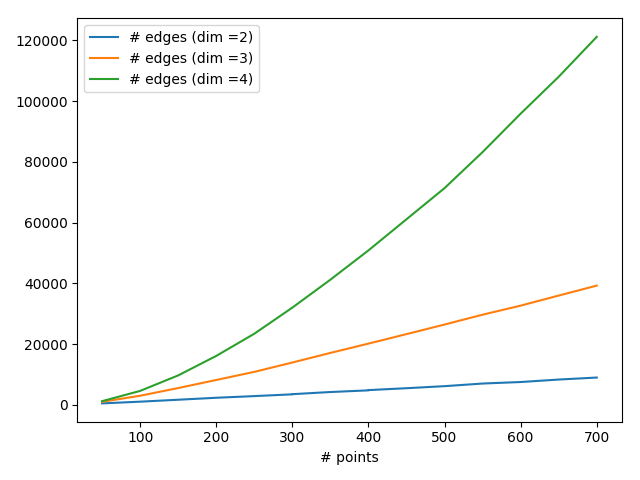
Figure 4: Results of blind greedy spanner for different dimensions.

Figure 5: Comparison of the four variants of BlindRandom algorithm.

Figure 6: Number of edges in the blind greedy and greedy spanners for different values of $\varepsilon$. Data is for 400 normally distributed points in $\mathbb{R}^{2}$ and $\mathbb{R}^{3}$.

We tested the algorithm for $\varepsilon\in\Set{0.01,0.1,0.2,0.5}$ on the following sets of points in dimensions $d=2,3,4,5$:

1. In the uniform test set points are sampled uniformly at random from the unit cube in $\mathbb{R}^{d}$.

2. In the normal test set points are sampled from the standard normal distribution in $\mathbb{R}^{d}$.

3. In the clustered test set we first sample cluster centers uniformly at random from $[0,10000]^{d}$, and then we add normally distributed noise around each of the centers. The number of clusters is chosen so that each cluster contains 50 points.

4. The test set exp consists of points of the form $(2^{\xi_{1}},\dots,2^{xi_{d}})$, where $\xi_{i}$’s are i.i.d. random variables with uniform distribution on $[1,25]$.

In all experiments the algorithms that we tested compared in the same way, so we only present results for the uniform point set in dimension 2.

Figure 2 shows the number of edges of the spanner for various variants of blind and non-blind spanner constructions. Note that for all blind spanner variants, the number of computed distances is equal to the spanner size, while for the non-blind greedy spanner, this number is always $\binom{n}{2}$ and for WPSD it is lower bounded by the size of the spanner. We can see that, even though none of the blind spanners can produce spanners of the same quality (i.e., sparse) as the standard greedy algorithm, BlindGreedy and all variants of BlindRandom perform significantly better than both variants of BlindQuasiSorted. Figure 3 shows the ratio of the number of edges to the number of points. The ideal behavior is demonstrated by the non-blind greedy spanner, for which this ratio stays practically constant, confirming the linear growth. None of the blind algorithms seems to have this property, but among them the blind greedy spanner is the best one. If we assume that the number of edges is proportional to $n^{\alpha}$, then we can try to estimate $\alpha$ by linear regression (after taking $\log$). We give in the table 1 the estimated exponents $\alpha$ for BlindGreedy and standard greedy algorithms. Note that even for the greedy algorithm these estimated exponents can be significantly larger than 1, which is explained by the fact that the number of points on which we computed spanners is not large enough to clearly see the linear dependence.

dimension	Greedy (non-blind)	Blind greedy
2	1.08	1.12
3	1.24	1.41
4	1.42	1.77

Table 1: Estimated exponents in the $|E|=C|V|^{\alpha}$ dependence of the number of edges on the number of points. The data is for $\varepsilon=0.1$ and for uniform points.

As for different variants of the BlindRandom algorithm, we note that their performance is almost the same, and the algorithm works significantly better than QuasiSorted variants, but obviously worse than the blind greedy variant. There is a consistent, though small, difference between the variants that do not force lower bounds first and the other two variants of the BlindRandom (see Figure 5).

WSPD spanners performed poorly in our experiments on non-clustered data, while the plots in the extensive experimental study Farshi and Gudmundsson (2009) show that WSPD spanners are very sparse, outperformed only by the greedy algorithm. We implemented two versions of WSPD: one for the Euclidean case, using quadtrees and the algorithm from Har-Peled (2011), and WSPD for general metric spaces with cover trees (using the base $\tau=1.3$). They both give similar results, and we can only conclude that the advantage of WSPD shows up on larger point sets than the ones we deal with. The paper Farshi and Gudmundsson (2009) contains experiments for up to 30000 points, and our blind algorithms, which have at least cubic complexity in the number of points, are infeasible for such $n$.

We also tested higher dimensions and show the results for the best algorithm, BlindGreedy, in dimensions 2, 3 and 4 in the plot 4. We can see that already in dimension 4, it produces a graph with roughly $\frac{1}{2}\binom{n}{2}$ edges for $700$ points, which clearly shows some degrading for higher dimensions. Still, we remark that the WSPD spanner remains worse also in the higher-dimensional setup.

The plot in Figure 6 compares the BlindGreedy and Greedy algorithms on uniform point sets for different choices of $\varepsilon$. We can see that dependence on $\varepsilon$ is approximately the same for both algorithms. Since it is not cleary seen from the picture, we also note that the ratio of the number of edges decreases for smaller values of $\varepsilon$: for $\varepsilon=2$ the blind greedy spanner contains almost 6 times more edges than the greedy spanner, while for $\varepsilon=1/32$ the ratio is 2.6

Summing up, we can conclude from the experiments that the BlindGreedy algorithm performs rather well, but also BlindRandom algorithm reduces the amount of computed distances substantially, especially if we enforce having non-zero lower bounds first. If the goal is to reduce the number of distance computations, these method seem to be more suitable than a WSPD spanner. Since the linear spanner size of WSPDs does not show up in the experiments because of the relatively small values of $n$ tested, the experiments are not conclusive regarding the asymptotic size of the blind spanners. Another noteworthy fact is that quasi-sorted variants produce spanners which are much closer to the complete graph (BlindQuasiSortedGreedy is worse, requiring all the edges). It would seem plausible that, if we have access to approximate value of the distance, we could exploit this in the spanner construction, but we could not find a working heuristic.

5 Approximate nearest neighbors

We consider the standard problem of finding an approximate nearest neighbor: given $n$ points $P=\Set{p_{1},\dots,p_{n}}$, a query point $q$ and a real number $\varepsilon>0$, find $p_{i}$ such that $\delta(p_{i},q)\leq(1+\varepsilon)\min_{k}\delta(q,p_{k})$. This notation will be fixed throughout this section, and we shall also use the shorthand notation

$$r_{i}:=\delta(p_{i},q).$$

We assume for simplicity that all exact pairwise distances $\delta(p_{i},p_{j})$ are already computed (a slight modification of the algorithm can also be applied if only a spanner is available). Our goal is to reduce the number of computed distances $\delta(p_{i},q)$.

Our approach can be summarized as follows. Fix a random permutation of the points of $P$ and consider the points in that order (to simplify notation, we re-index them, so the order is again $p_{1},\dots,p_{n}$). During the loop, we maintain lower bounds of each $p_{i}$ to the query point $q$, which are initially all set to $0$. We also remember the closest neighbor $c$ that we have seen so far and its distance $v$ to $q$. We refer to the point $c$ as the candidate. We maintain the invariant that $c$ is an approximate nearest neighbor to $q$ for the points $\{p_{1},\ldots,p_{i}\}$. When reaching the point $p_{i}$, we check whether the lower bound $a_{i}$ satisfies $a_{i}\geq\frac{v}{1+\varepsilon}$. If so, $c$ remains an approximate nearest neighbor and we do not query the distance of $p_{i}$ to $q$. Otherwise, we compute $\delta(p_{i},q)$ and update the lower bounds of all points according to the newly computed distance. If $p_{i}$ is closer to $q$ than $c$, we update $c$ and $v$ accordingly. At the end of the loop, $c$ is an approximate nearest neighbor. The pseudocode of the procedure follows.

function ApproximateNearestNeighbor($P,q,\varepsilon$)

     $[p_{1},\dots,p_{n}]\leftarrow\mbox{random permutation of }P$

      $a_{i}\leftarrow 0$ for $i=1,\ldots,n$ $\triangleright$ $a_{i}$ is lower bound for $\delta(p_{i},q)$

     $c\leftarrow p_{1},\quad v\leftarrow\delta(p_{1},q)$ $\triangleright$ $c$ keeps the current candidate

     UpdateBounds($p_{1},v$)

     for $i=2\dots n$ do

         if $a_{i}\geq\frac{v}{1+\varepsilon}$ then

              continue

         else

              Compute $r_{i}=\delta(p_{i},q)$

              UpdateBounds($p_{i},r_{i}$)

              if $r_{i}<v$ then

                  $c\leftarrow p_{i},\quad v\leftarrow r_{i}$                             

     return $c,v$

We remark that we obtain an exact nearest neighbor algorithm when setting $\varepsilon$ to $0$, which means replacing the condition in the if-statement of the loop with $a_{i}\geq v$.

The procedure to maintain the lower bounds $a_{i}$ is very simple and follows directly from triangle inequality.

procedure UpdateBounds($p_{i},r_{i}$)

     for $k=i+1,\dots,n$ do

         $a_{k}\leftarrow\max(a_{k},|\delta(p_{i},p_{k})-r_{i}|)$      

Theorem 2.

If $(\mathcal{M},\delta)$ is a doubling space, then, for any fixed $\varepsilon>0$ the algorithm computes $O(\log n)$ distances $\delta(p_{i},q)$ in expectation.

Towards the proof, we will use the following geometric lemma which can be summarized as follows: if $\delta(p_{i},q)$ is computed in the algorithm, further distance computations of points very close to $p_{i}$ or very far from $p_{i}$ will be avoided.

Lemma 3.

Assume $r_{i}=\delta(p_{i},q)$ is computed in the algorithm, and let $j>i$.

1. If $\delta(p_{i},p_{j})\geq(1+\frac{1}{1+\varepsilon})r_{i}$, the algorithm will not compute the distance of $p_{j}$ to $q$.

2. If $\delta(p_{i},p_{j})\leq\frac{\varepsilon}{1+\varepsilon}r_{i}$, the algorithm will not compute the distance of $p_{j}$ to $q$.

Proof.

Figure 7: First two steps of the ANN algorithm. First $p_{1}$ is chosen as the current candidate, and we must compute $\delta(p_{2},q)$. After that the algorithm will not compute distance to any of the points inside the heavily shaded ball or outside the lightly shaded ball that are centered at $p_{2}$, because their lower bounds allow us to discard them. Note that the point $p_{5}$, which is closer to $q$ than $p_{1}$, also will not be a candidate, and at least one of the points $p_{6},p_{7},p_{8},p_{9}$ in the annulus between the dashed and solid circle, which are further from $q$ than $p_{5}$, will be chosen as $c$. This shows that in our algorithm the distance from the candidate to $q$ can drop slower than in the bruteforce algorithm, thus Theorem 2 does not immediately follow from standard backwards analysis. The small black ball between the dashed circle and the solid circle has radius $v_{1}\varepsilon/(1+\varepsilon)$; it is the ball that we use in the packing argument, because it is smaller than any of the lightly shaded balls that correspond to points like $p_{2}$ and $p_{4}$, that is, the points that do not improve $v$.

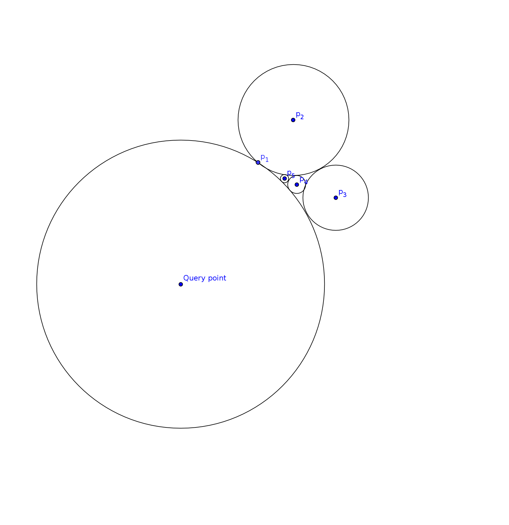
Figure 8: Example of point set where exact nearest neighbor search cannot be accelerated by maintaining bounds. The exact nearest neighbor is the point $p_{1}$, next point $p_{i}$ is placed in the curvilinear triange formed by the balls around the query point, $p_{2}$ and $p_{i-1}$. Even verifying that $p_{1}$ is the true nearest neighbor cannot be done without computing all distances $\delta(p_{i},q)$. Indeed, every computed $\delta(p_{i},q)$ allows to exclude the region in the corresponding ball around $p_{i}$, but all these balls contain only one $p_{i}$.

The algorithm computes $r_{i}$ by assumption and updates all lower bounds. For $p_{j}$, it sets $a_{j}\leftarrow\max(a_{j},|\delta(p_{i},p_{j})-r_{i}|)$. If $\delta(p_{i},p_{j})\geq(1+\frac{1}{1+\varepsilon})r_{i}$, it follows that

$$a_{j}\geq(1+\frac{1}{1+\varepsilon})r_{i}-r_{i}=\frac{r_{i}}{1+\varepsilon}.$$

Likewise, if $\delta(p_{i},p_{j})\leq\frac{\varepsilon}{1+\varepsilon}r_{i}$,

$$a_{j}\geq r_{i}-\delta(p_{i},p_{j})\geq r_{i}-\frac{\varepsilon}{1+\varepsilon}r_{i}=\frac{r_{i}}{1+\varepsilon}.$$

In both cases, after the point $p_{i}$ is handled, $v\leq r_{i}$ clearly holds. Since $v$ is only decreasing and $a_{j}$ is only increasing in the algorithm, it follows that $a_{j}\geq\frac{v}{1+\varepsilon}$ when $p_{j}$ is handled, so the algorithm proceeds without a distance computation. ∎

In what follows, we let $c_{i}$ denote the candidate at the end of the $i$-th iteration of the loop, and $v_{i}$ the distance to $\delta(c_{i},q)$, $i=1,\dots,n$. Clearly, $v_{1},\ldots,v_{n}$ is a decreasing sequence. With the previous lemma, we can derive an upper bound for the number of distance computations in an arbitrary subsequence of $p_{1},\ldots,p_{n}$ as follows.

Lemma 4.

Among the points $p_{k},\ldots,p_{\ell}$ with $1\leq k<\ell\leq n$, the algorithm computes at most

$$\left(\frac{4(2+\varepsilon)v_{k}}{\varepsilon v_{\ell}}\right)^{d}$$

distances to $q$.

Proof.

By the first part of Lemma 3, every point in $p_{k},\ldots,p_{\ell}$ whose distance to $q$ is queried lies in the ball of radius $(1+\frac{1}{1+\varepsilon})v_{k}=\frac{2+\varepsilon}{1+\varepsilon}v_{k}$ around $c_{k}$. Moreover, if the distance of two points $p_{i}$ and $p_{j}$ with $k\leq i<j\leq\ell$ is computed, the second part of Lemma 3 implies that $\delta(p_{i},p_{j})>\frac{\varepsilon}{1+\varepsilon}r_{i}\geq\frac{\varepsilon}{1+\varepsilon}v_{\ell}$. Hence, all points in $p_{k},\ldots,p_{\ell}$ for which the algorithm computes the distance have a pairwise distance of at least $\frac{\varepsilon}{1+\varepsilon}v_{\ell}$. The statement follows by applying Lemma 1. ∎

A consequence of the lemma is that as long as a candidate $c$ is fixed in the algorithm, the number of computed distances is a constant (since $v_{k}=v_{\ell}$). This means that to prove Theorem 2, it would suffice to show that the candidate changes only a logarithmic number of times in expectation. While we have not found a simple proof for this claim, we can prove the statement with a slight variant of that argument.

Proof.

(of Theorem 2) In the sequence $p_{1},\ldots,p_{n}$, let $p_{k}$ be a point such that $r_{i}<r_{k}$ for all $1\leq i\leq k-1$. We call an element of this form a minimum of the sequence. A standard backwards analysis argument Seidel (1993) shows that the probability of $p_{k}$ being a minimum is at most $1/k$, so that the number of minima in the sequence is $O(\log n)$ in expectation.

Note that for $\varepsilon>0$, a minimum $p_{k}$ is not necessarily the candidate $c_{k}$ because a previous point in the sequence close to $p_{k}$ might have caused the lower bound $a_{k}$ to be in the interval $[\frac{v_{k}}{1+\varepsilon},v_{k}]$, which leads to not computing the distance $r_{k}$. However, it is true that $v_{k}\leq(1+\varepsilon)r_{k}$, because otherwise, $c_{k}$ would not be an approximate nearest neighbor of $\{p_{1},\ldots,p_{k}\}$.

Now, let $p_{k}$, $p_{\ell}$ be two consecutive minima in the sequence (we also allow that $\ell=n+1$ if $k$ is the last minimum in the sequence). Note that $v_{\ell-1}\geq r_{k}$ because each $v_{j}$ is equal to $r_{i}$ for some $i\leq j$, and in the sequence $r_{1},\ldots,r_{\ell-1}$, $r_{k}$ is minimal by construction. Using Lemma 4, the number of distance computations among the points $p_{k},\ldots,p_{\ell-1}$ is at most

$$\left(\frac{4(2+\varepsilon)v_{k}}{\varepsilon v_{\ell-1}}\right)^{d}\leq\left(\frac{4(2+\varepsilon)(1+\varepsilon)r_{k}}{\varepsilon r_{k}}\right)^{d}=\left(\frac{4(2+\varepsilon)(1+\varepsilon)}{\varepsilon}\right)^{d},$$

which is a constant depending only of $\varepsilon$ and $d$, irrespective of the length of the sequence. Since $p_{1},\ldots,p_{n}$ decomposes into $O(\log n)$ such sequences in expectation, the result follows. ∎

We point out that the proof fails for $\varepsilon=0$ because in that case, we cannot exclude an $\varepsilon$-ball of close-by points as in the second part of Lemma 3, and the packing argument fails. Indeed, as the example in Figure 8 shows, there are point sets where the expected number of distance computations for exact nearest neighbor is linear.

Finally, we remark that a fast $2$-approximation algorithm for $\delta$ would lead to a straight-forward optimization: compute a $2$-approximation of $\delta(p_{i},q)$ for all $1\leq i\leq n$ and let $m$ denote the minimal approximate distance encountered. Then, we can discard all points whose approximate distance is larger than $2m$, and run the above algorithm on the remaining points.

6 Experiments on approximate nearest neighbors

In order to experimentally evaluate the performance of our algorithm, we generate random point sets and random query points, and for each query point run the algorithm 10 times. The average number of distances to the query point that were actually computed is the measure that we are interested in. We average the results over 10 different instances of the point set and query point in order to see the trend clearer; thus each point on the plots in this section is the result of averaging of 100 runs of the code (10 instances, 10 random permutations per instance).

Figure 9: Ratio $\log(\mbox{computed distances})/n$ for ANN algorithm. Data is for uniformly distributed points.

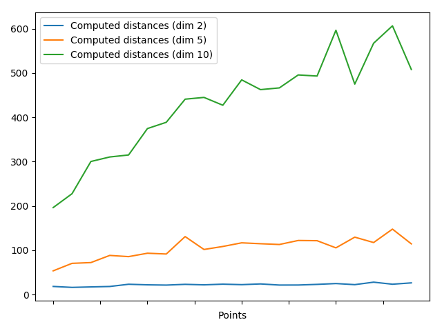
Figure 10: Number of computed distances for different dimensions. Points are chosen uniformly, $\varepsilon=0.01$.

We used the following methods of generating random points:

1. Uniform. Points are sampled uniformly at random from the unit cube in $\mathbb{R}^{d}$.

2. Normal. Points are sampled from the normal distribution.

Query points were sampled from the uniform distribution on the cube $[-10,10]^{d}$ and from the normal distribution centered at the origin with scale 100, thus we get query points that are "inside" the point set and also "outside". We sample data in dimensions up to 20 and for $\varepsilon\in\Set{0.001,0.005,0.01,0.05,0.1}$, the maximal number of points is $30,000$.

In order to empirically verify the upper bound $O(\log n)$, we plot the number of computed distances divided by the logarithm of the number of points in figure 9 (for $d=2$). We see that this ratio, though fluctuating a lot, remains in the interval $[1,4]$. This not just confirms the theoretical upper bound, but also shows that the algorithm in the low-dimensional case really computes only a very small number of distances to the query point. As expected, in high dimensions the algorithm does not perform as well. In Figure 10 we plot the average number of computed distances for $d=2,5,10$. While for $d=2$ the growth is hardly noticeable, for $d=10$ the sublinearity of the growth becomes clear only when the number of points is relatively large, approaching 30000.

7 Conclusion and future work

We have introduced a new cost model for the analysis of algorithms for metric spaces that fits the situation that computing an individual distance is more costly than other types of primitive operations. Our theoretical and experimental results are under the usual assumption that the metric space has a low doubling dimension. However, in our motivating example of collections of persistence diagrams or Reeb graphs, this assumption does not hold. For instance, the space of persistence diagrams has an infinite doubling dimension. Nevertheless, realistic data sets are usually not just a random sample in that infinite-dimensional space, but have structures (e.g. clusters of close-by diagrams) which should be favorable for our approach We plan to consider the quality of our algorithms for persistence diagrams as future work.

On the theoretical side, the obvious next question is whether our strategy for blind spanners yields a linear spanner in expectation. Our experiments are not conclusive enough in this respect to make this conjecture yet. However, it has been brought to our attention that the size of the blind spanner is bounded by the weight of the WSPD which is the sum of the cardinalities of all pairs in a WSPD. The weight of a WSPD can be quadratic, but preliminary experimental evaluation on worst-case examples do not show such a quadratic behavior. Therefore, we postpone the theoretical analysis of the spanner construction to an extended version of this article.

The existence of a $2$-approximation algorithm did not help us to significantly reduce the number of exact distance computations, although it seems obvious that knowing the all approximate distances is useful. We pose the question what heuristic could make more use of this feature.

References

- Althöfer et al. (1993) Ingo Althöfer, Gautam Das, David Dobkin, Deborah Joseph, and José Soares. On sparse spanners of weighted graphs. Discrete & Computational Geometry, 9(1):81–100, 1993.
- Bauer et al. (2014) Ulrich Bauer, Xiaoyin Ge, and Yusu Wang. Measuring distance between reeb graphs. In Proceedings of the thirtieth annual symposium on Computational geometry, page 464. ACM, 2014.
- Beygelzimer et al. (2006) Alina Beygelzimer, Sham Kakade, and John Langford. Cover trees for nearest neighbor. In Proceedings of the 23rd International Conference on Machine Learning, ICML ’06, pages 97–104, New York, NY, USA, 2006. ACM. ISBN 1-59593-383-2. doi: 10.1145/1143844.1143857. URL http://doi.acm.org/10.1145/1143844.1143857.
- Biasotti et al. (2008) S. Biasotti, D. Giorgi, M. Spagnuolo, and B. Falcidieno. Reeb graphs for shape analysis and applications. Theoretical Computer Science, 392(13):5 – 22, 2008. ISSN 0304-3975. doi: http://dx.doi.org/10.1016/j.tcs.2007.10.018. URL http://www.sciencedirect.com/science/article/pii/S0304397507007396. Computational Algebraic Geometry and Applications.
- Callahan and Kosaraju (1995a) Paul B. Callahan and S. Rao Kosaraju. A decomposition of multidimensional point sets with applications to k-nearest-neighbors and n-body potential fields. J. ACM, 42(1):67–90, January 1995a. ISSN 0004-5411. doi: 10.1145/200836.200853. URL http://doi.acm.org/10.1145/200836.200853.
- Callahan and Kosaraju (1995b) Paul B Callahan and S Rao Kosaraju. A decomposition of multidimensional point sets with applications to k-nearest-neighbors and n-body potential fields. Journal of the ACM (JACM), 42(1):67–90, 1995b.
- Cohen-Steiner et al. (2007) David Cohen-Steiner, Herbert Edelsbrunner, and John Harer. Stability of persistence diagrams. Discrete & Computational Geometry, 37(1):103–120, 2007.
- De Silva et al. (2016) Vin De Silva, Elizabeth Munch, and Amit Patel. Categorified reeb graphs. Discrete & Computational Geometry, 55(4):854–906, 2016.
- Di Fabio and Landi (2016) Barbara Di Fabio and Claudia Landi. The edit distance for reeb graphs of surfaces. Discrete & Computational Geometry, 55(2):423–461, 2016.
- Edelsbrunner et al. (2002) H. Edelsbrunner, D. Letscher, and A. Zomorodian. Topological persistence and simplification. Discrete & Computational Geometry, 28(4):511–533, 2002. ISSN 01795376. doi: 10.1007/s00454-002-2885-2.
- Farshi and Gudmundsson (2009) Mohammad Farshi and Joachim Gudmundsson. Experimental study of geometric t-spanners. Journal of Experimental Algorithmics (JEA), 14:3, 2009.
- Har-Peled and Mendel (2006) S. Har-Peled and M. Mendel. Fast construction of nets in low dimensional metrics and their applications. SIAM Journal on Computing, 35:1148–1184, 2006.
- Har-Peled (2011) Sariel Har-Peled. Geometric approximation algorithms. Number 173. American Mathematical Soc., 2011.
- Krauthgamer and Lee (2005) Robert Krauthgamer and James R Lee. The black-box complexity of nearest-neighbor search. Theoretical Computer Science, 348(2-3):262–276, 2005.
- Rubner et al. (2000) Yossi Rubner, Carlo Tomasi, and Leonidas J Guibas. The earth mover’s distance as a metric for image retrieval. International journal of computer vision, 40(2):99–121, 2000.
- Seidel (1993) Raimund Seidel. Backwards analysis of randomized geometric algorithms. In Janos Pach, editor, New Trends in Discrete and Computational Geometry. Springer, 1993.
- Smid (2009) Michiel Smid. Efficient algorithms. chapter The Weak Gap Property in Metric Spaces of Bounded Doubling Dimension, pages 275–289. Springer-Verlag, Berlin, Heidelberg, 2009. ISBN 978-3-642-03455-8. doi: 10.1007/978-3-642-03456-5_19. URL http://dx.doi.org/10.1007/978-3-642-03456-5_19.