Don’t Jump Through Hoops and Remove Those Loops: SVRG and Katyusha are Better Without the Outer Loop

Abstract

The stochastic variance-reduced gradient method (SVRG) and its accelerated variant (Katyusha) have attracted enormous attention in the machine learning community in the last few years due to their superior theoretical properties and empirical behaviour on training supervised machine learning models via the empirical risk minimization paradigm. A key structural element in both of these methods is the inclusion of an outer loop at the beginning of which a full pass over the training data is made in order to compute the exact gradient, which is then used in an inner loop to construct a variance-reduced estimator of the gradient using new stochastic gradient information. In this work we design loopless variants of both of these methods. In particular, we remove the outer loop and replace its function by a coin flip performed in each iteration designed to trigger, with a small probability, the computation of the gradient. We prove that the new methods enjoy the same superior theoretical convergence properties as the original methods. For loopless SVRG, the same rate is obtained for a large interval of coin flip probabilities, including the probability $\nicefrac{{1}}{{n}}$, where $n$ is the number of functions. This is the first result where a variant of SVRG is shown to converge with the same rate without the need for the algorithm to know the condition number, which is often unknown or hard to estimate correctly. We demonstrate through numerical experiments that the loopless methods can have superior and more robust practical behavior.

1 Introduction

Empirical risk minimization (aka finite-sum) problems form the dominant paradigm for training supervised machine learning models such as ridge regression, support vector machines, logistic regression, and neural networks. In its most general form, a finite sum problem has the form

$$\textstyle\min_{x\in\mathbb{R}^{d}}f(x)\overset{\text{def}}{=}\tfrac{1}{n}\sum\limits_{i=1}^{n}f_{i}(x)\;,$$ (1)

where $n$ refers to the number of training data points (e.g., videos, images, molecules), $x$ is the vector representation of a model using $d$ features, and $f_{i}(x)$ is the loss of model $x$ on data point $i$.

Variance-reduced methods. One of the most remarkable algorithmic breakthroughs in recent years was the development of variance-reduced stochastic gradient algorithms for solving (1). These methods are significantly faster than SGD [18, 17, 27] in theory and practice on convex and strongly convex problems, and faster in theory on several classes on nonconvex problems (unfortunately, these methods are no yet successful in training production-grade neural networks).

Two of the most notable and popular methods belonging to the family of variance-reduced methods are SVRG [12] and its accelerated variant known as Katyusha [1]. The latter method accelerates the former via the employment of a novel “negative momentum” idea. Both of these methods have a double loop design. At the beginning of the outer loop, a full pass over the training data is made to compute the gradient of $f$ at a reference point $w^{k}$, which is chosen as the freshest iterate (SVRG) or a weighted average of recent iterates (for Katyusha). This gradient is then used in the inner loop to adjust the stochastic gradient $\nabla f_{i}(x^{k})$, where $i$ is sampled uniformly at random from $[n]\overset{\text{def}}{=}\{1,2,\dots,n\}$, and $x^{k}$ is the current iterate, so as to reduce its variance. In particular, both SVRG and Katyusha perform the adjustment $g^{k}=\nabla f_{i}(x^{k})-\nabla f_{i}(w^{k})+\nabla f(w^{k}).$ Note that, like $\nabla f_{i}(x^{k})$, the new search direction $g^{k}$ is an unbiased estimator of $\nabla f(x^{k})$. Indeed,

$${\rm E}\left[g^{k}\right]=\nabla f(x^{k})-\nabla f(w^{k})+\nabla f(w^{k})=\nabla f(x^{k}).$$ (2)

where the expectation is taken over random choice of $i\in[n]$. However, it turns out that as the methods progress, the variance of $g^{k}$, unlike that of $\nabla f_{i}(x^{k})$, progressively decreases to zero. The total effect of this is significantly faster convergence.

Converegnce of SVRG and Katyusha for $L$–smooth and $\mu$–strongly convex functions. For instance, consider the regime where $f_{i}$ is $L$–smooth for each $i$, and $f$ is $\mu$–strongly convex:

Assumption 1.1 ($L$–smoothness).

Functions $f_{i}:\mathbb{R}^{d}\rightarrow\mathbb{R}$ are $L$–smooth for some $L>0$:

$$f(y)\leq f(x)+\left<\nabla f(x),y-x\right>+\tfrac{L}{2}\left\lVert y-x\right\rVert^{2},\qquad\forall x,y\in\mathbb{R}^{d}.$$ (3)

Assumption 1.2 ($\mu$–strong convexity).

Function $f:\mathbb{R}^{d}\rightarrow\mathbb{R}$ is $\mu$–strongly convex for $\mu>0$:

$$f(y)\geq f(x)+\left<\nabla f(x),y-x\right>+\tfrac{\mu}{2}\left\lVert y-x\right\rVert^{2},\qquad\forall x,y\in\mathbb{R}^{d}.$$ (4)

In this regime, the iteration complexity of SVRG is ${\cal O}\left(\left(n+\nicefrac{{L}}{{\mu}}\right)\log\nicefrac{{1}}{{\epsilon}}\right),$ which is a vast improvement on the linear rate of gradient descent (GD), which is ${\cal O}\left(\nicefrac{{nL}}{{\mu}}\log\nicefrac{{1}}{{\epsilon}}\right)$, and on the sublinear rate of SGD, which is ${\cal O}(\nicefrac{{L}}{{\mu}}+\nicefrac{{\sigma^{2}}}{{\mu^{2}\epsilon}})$, where $\sigma^{2}=\nicefrac{{1}}{{n}}\sum_{i}\|\nabla f_{i}(x^{*})\|^{2}$ and $x^{*}$ is the (necessarily unique) minimizer of $f$. On the other hand, Katyusha enjoys the accelerated rate ${\cal O}((n+\sqrt{\nicefrac{{nL}}{{\mu}}})\log\nicefrac{{1}}{{\epsilon}}),$ which is superior to that of SVRG in the ill-conditioned regime where $\nicefrac{{L}}{{\mu}}\geq n$. This rate has been shown to be optimal in a certain precise sense [19].

In the past several years, an enormous effort of the machine learning and optimization communities was exerted into designing new efficient variance-reduced methods algorithms to tackle problem (1). These developments have brought about a renaissance in the field. The historically first provably variance-reduced method, the stochastic average gradient (SAG) method of [23, 24], was awarded the Lagrange prize in continuous optimization in 2018. The SAG method was later modified to an unbiased variant called SAGA [6], achieving the same theoretical rates. Alternative variance-reduced method include MISO [16], FINITO [7], SDCA [25], dfSDCA [4], AdaSDCA [3], QUARTZ [22], SBFGS [9], SDNA [21], SARAH [20] and S2GD [14], mS2GD [13], RBCN [8], JacSketch [10] and SAGD [2]. Accelerated variance-reduced method were developed in [26], [5], [28] and [29].

2 Contributions

As explained in the introduction, a trade-mark structural feature of SVRG and its accelerated variant, Katyusha, is the presence of the outer loop in which a full pass over the data is made. However, the presence of this outer loop is the source of several issues. First, the methods are harder to analyze. Second, one needs to decide at which point the inner loop is terminated and the outer loop entered. For SVRG, the theoretically optimal inner loop size depends on both $L$ and $\mu$. However, $\mu$ is not always known. Moreover, even when an estimate is available, as is the case in regularized problems with an explicit strongly convex regularizer, the estimate can often be very loose. Because of these issues, one often chooses the inner loop size in a suboptimal way, such as by setting it to $n$ or ${\cal O}(n)$.

Two loopless methods. In this paper we address the above issues by developing loopless variants of both SVRG and Katyusha; we refer to them as L-SVRG and L-Katyusha, respectively. In these methods, we dispose of the outer loop and replace its role by a biased coin-flip, to be performed in every step of the methods, used to trigger the computation of the gradient $\nabla f(w^{k})$ via a pass over the data. In particular, in each step, with (a small) probability $p>0$ we perform a full pass over data and update the reference gradient $\nabla f(w^{k})$. With probability $1-p$ we keep the previous reference gradient. This procedure can alternatively be interpreted as having an outer loop of a random length. However, the resulting methods are easier to write down, comprehend and analyze.

Fast rates are preserved. We show that L-SVRG and L-Katyusha enjoy the same fast theoretical rates as their loopy forefathers. Our proofs are different and the complexity results more insightful.

For L-SVRG with fixed stepsize $\eta=\nicefrac{{1}}{{6L}}$ and probability $p=\nicefrac{{1}}{{n}}$, we show (see Theorem 3.5) that for the Lyapunov function

$$\textstyle\Phi^{k}\overset{\text{def}}{=}\left\lVert x^{k}-x^{*}\right\rVert^{2}+\tfrac{4\eta^{2}}{pn}\sum\limits_{i=1}^{n}\left\lVert\nabla f_{i}(w^{k})-\nabla f_{i}(x^{*})\right\rVert^{2}.$$ (5)

we get ${{\rm E}}\left[\Phi^{k}\right]\leq\epsilon\Phi^{0}$ as long as $k={\cal O}\left(\left(n+\nicefrac{{L}}{{\mu}}\right)\log\nicefrac{{1}}{{\epsilon}}\right).$ In contrast, the classical SVRG result shows convergence of the expected functional suboptimality ${{\rm E}}\left[f(x^{k})-f(x^{*})\right]$ to zero at the same rate. Note that the classical result follows from our theorem by utilizing the inequality $f(x^{k})-f(x^{*})\leq\nicefrac{{L}}{{2}}\|x^{k}-x^{*}\|^{2},$ which is a simple consequence of $L$–smoothness. However, our result provides a deeper insight into the behavior of the method. In particular, it follows that the gradients $\nabla f_{i}(w^{k})$ at the reference points $w^{k}$ converge to the gradients at the optimum. This is a key intuition behind the workings of SVRG, one not revealed by the classical analysis. Hereby we close the gap in the theoretical understanding of the the SVRG convergence mechanism. Moreover, our theory predicts that as long as $p$ is chosen in the (possibly very large) interval

$$\min\left\{\nicefrac{{c}}{{n}},\nicefrac{{c\mu}}{{L}}\right\}\leq p\leq\max\left\{\nicefrac{{c}}{{n}},\nicefrac{{c\mu}}{{L}}\right\},$$ (6)

where $c=\Theta(1)$, L-SVRG will enjoy the optimal complexity ${\cal O}\left(\left(n+\nicefrac{{L}}{{\mu}}\right)\log\nicefrac{{1}}{{\epsilon}}\right)$. In the ill-conditioned regime $\nicefrac{{L}}{{\mu}}\gg n$, for instance, we roughly have $p\in[\nicefrac{{\mu}}{{L}},\nicefrac{{1}}{{n}}]$. This is in contrast with the (loopy/standard) SVRG method the outer loop of which needs to be of the size $\approx\nicefrac{{L}}{{\mu}}$. To the best of our knowledge, SVRG does not enjoy this rate for an outer loop of size $n$ (or any value independent of $\mu$, which is often not known in practice), even though this is the setting most often used in practice. Several authors have tried to establish such a result, but without success. We thus answer an open problem since 2013, the inception of SVRG.

For L-Katyusha with stepsize $\eta=\frac{\theta_{2}}{(1+\theta_{2})\theta_{1}}$ we show convergence of the Lyapunov function

$$\Psi^{k}={\cal Z}^{k}+{\cal Y}^{k}+{\cal W}^{k},$$ (7)

where ${\cal Z}^{k}=\tfrac{L(1+\eta\sigma)}{2\eta}\left\lVert z^{k}-x^{*}\right\rVert^{2}$, ${\cal Y}^{k}=\tfrac{1}{\theta_{1}}(f(y^{k})-f(x^{*}))$, and ${\cal W}^{k}=\tfrac{\theta_{2}(1+\theta_{1})}{p\theta_{1}}(f(w^{k})-f(x^{*}))$, and where $x^{k},y^{k}$ and $w^{k}$ are iterates produced by the method, with the parameters defined by $\sigma=\nicefrac{{\mu}}{{L}}$, $\theta_{1}=\min\{\sqrt{\nicefrac{{2\sigma n}}{{3}}},\nicefrac{{1}}{{2}}\}$, $\theta_{2}=\nicefrac{{1}}{{2}}$, $p=\nicefrac{{1}}{{n}}$. Our main result (Theorem 4.6) states that ${{\rm E}}\left[\Psi^{k}\right]\leq\epsilon\Psi^{0}$ as long as $k={\cal O}((n+\sqrt{\nicefrac{{nL}}{{\mu}}})\log\nicefrac{{1}}{{\epsilon}}).$

Simplified analysis. Advantage of the loopless approach is that a single iteration analysis is sufficient to establish convergence. In contrast, one needs to perform elaborate aggregation across the inner loop to prove the convergence of the original loopy methods.

Superior empirical behaviour. We show through extensive numerical testing on both synthetic and real data that our loopless methods are superior to their loopy variants. We show through experiments that L-SVRG is very robust to the choice of $p$ from the optimal interval (6) predicted by our theory. Moreover, even the worst case for L-SVRG outperforms the best case for SVRG. This shows how further randomization can significantly speed up and stabilize the algorithm.

Notation. Throughout the whole paper we use conditional expectation ${\rm E}\left[{\cal X}\;|\;x^{k},w^{k}\right]$ for L-SVRG and ${\rm E}\left[{\cal X}\;|\;y^{k},z^{k},w^{k}\right]$ for L-Katyusha, but for simplicity we will denote these expectations as ${\rm E}\left[{\cal X}\right]$. If ${\rm E}\left[{\cal X}\right]$ refers to unconditional expectation, it is directly mentioned.

3 Loopless SVRG (L-SVRG)

In this section we describe in detail the Loopless SVRG method (L-SVRG), and its convergence.

The algorithm. The L-SVRG method, formalized as Algorithm 1, is inspired by the original SVRG [12] method. We remove the outer loop present in SVRG and instead use a probabilistic update of the full gradient. This update can be also seen in a way that outer loop size is generated by geometric distribution similar to [14, 15].

Algorithm 1 Loopless SVRG (L-SVRG)

  Parameters: stepsize $\eta>0$, probability $p\in(0,1]$

  Initialization: $x^{0}=w^{0}\in\mathbb{R}^{d}$

  for  $k=0,1,2,\ldots$  do

     $g^{k}=\nabla f_{i}(x^{k})-\nabla f_{i}(w^{k})+\nabla f(w^{k})$ ($i\in\{1,\ldots,n\}$ is sampled uniformly at random)

     $x^{k+1}=x^{k}-\eta g^{k}$

     $w^{k+1}=\begin{cases}x^{k}&\text{with probability }p\\ w^{k}&\text{with probability }1-p\end{cases}$

  end for

Note that the reference point $w^{k}$ (at which a full gradient is computed) is updated in each iteration with probability $p$ to the current iterate $x^{k}$, and is left unchanged with probability $1-p$. Alternatively, the probability $p$ can be seen as a parameter that controls the expected time before next full pass over data. To be more precise, the expected time before next full pass over data is $\nicefrac{{1}}{{p}}$. Intuitively, we wish to keep $p$ small so that full passes over data are computed rarely enough. As we shall see next, the simple choice $p=\nicefrac{{1}}{{n}}$ leads to complexity identical to that of original SVRG.

Convergence theory. A key role in the analysis is played by the gradient learning quantity

$$\textstyle{\cal D}^{k}\overset{\text{def}}{=}\tfrac{4\eta^{2}}{pn}\sum\limits_{i=1}^{n}\left\lVert\nabla f_{i}(w^{k})-\nabla f_{i}(x^{*})\right\rVert^{2}$$ (8)

and the Lyapunov function $\Phi^{k}\overset{\text{def}}{=}\left\lVert x^{k}-x^{*}\right\rVert^{2}+{\cal D}^{k}.$ The analysis involves four lemmas, followed by the main theorem. We wish to mention the lemmas as they highlight the way in which the argument works. All lemmas combined, together with the main theorem, can be proved on a single page, which underlines the simplicity of our approach.

Our first lemma upper bounds the expected squared distance of $x^{k+1}$ from $x^{*}$ in terms of the same distance but for $x^{k}$, function suboptimality, and variance of $g^{k}$.

Lemma 3.1.

We have

$$\begin{split}&{\rm E}\left[\left\lVert x^{k+1}-x^{*}\right\rVert^{2}\right]\leq(1-\eta\mu)\left\lVert x^{k}-x^{*}\right\rVert^{2}-2\eta(f(x^{k})-f(x^{*}))+\eta^{2}{\rm E}\left[\left\lVert g^{k}\right\rVert^{2}\right].\end{split}$$ (9)

In our next lemma, we further bound the variance of $g^{k}$ in terms of function suboptimality and ${\cal D}^{k}$.

Lemma 3.2.

We have

$$\begin{split}{\rm E}\left[\left\lVert g^{k}\right\rVert^{2}\right]\leq 4L(f(x^{k})-f(x^{*}))+\tfrac{p}{2\eta^{2}}{\cal D}^{k}.\end{split}$$ (10)

Finally, we bound ${\rm E}\left[{\cal D}^{k+1}\right]$ in terms of ${\cal D}^{k}$ and function suboptimality.

Lemma 3.3.

We have

$$\begin{split}{\rm E}\left[{\cal D}^{k+1}\right]\leq(1-p){\cal D}^{k}+8L\eta^{2}(f(x^{k})-f(x^{*})).\end{split}$$ (11)

Putting the above three lemmas together naturally leads to the following result involving Lyapunov function (5).

Lemma 3.4.

Let the step size $\eta\leq\nicefrac{{1}}{{6L}}$. Then for all $k\geq 0$ the following inequality holds:

$${\rm E}\left[\Phi^{k+1}\right]\leq(1-\eta\mu)\left\lVert x^{k}-x^{*}\right\rVert^{2}+\left(1-\nicefrac{{p}}{{2}}\right){\cal D}^{k}.$$ (12)

In order to obtain a recursion involving the Lyapunov function on the right-hand side of (12)

Theorem 3.5.

Let $\eta=\nicefrac{{1}}{{6L}}$, $p=\nicefrac{{1}}{{n}}$. Then ${\rm E}\left[\Phi^{k}\right]\leq\varepsilon\Phi^{0}$ as long as $k\geq{\cal O}\left(\left(n+\nicefrac{{L}}{{\mu}}\right)\log\nicefrac{{1}}{{\varepsilon}}\right).$

Proof.

As the corollary of Lemma 3.4 we have ${\rm E}\left[\Phi^{k}\right]\leq\max\left\{1-\eta\mu,1-\nicefrac{{p}}{{2}}\right\}\Phi^{k-1}.$ Setting $\eta=\nicefrac{{1}}{{6L}}$, $p=\nicefrac{{1}}{{n}}$ and unrolling conditional probability one obtains ${\rm E}\left[\Phi^{k}\right]\leq\max\left\{1-\nicefrac{{\mu}}{{6L}},1-\nicefrac{{1}}{{2n}}\right\}^{k}\Phi^{0},$ which concludes the proof. ∎

Note that the step size does not depend on the strong convexity parameter $\mu$ and yet the resulting complexity adapts to it.

Discussion. Examining (12), we can see that contraction of the Lyapunov function is $\max\{1-\eta\mu,1-\nicefrac{{p}}{{2}}\}$. Due to the limitation of $\eta\leq\nicefrac{{1}}{{6L}}$, the first term is at least $1-\nicefrac{{\eta}}{{6\mu}}$, thus the complexity cannot better than ${\cal O}\left(\nicefrac{{L}}{{\mu}}\log\nicefrac{{1}}{{\varepsilon}}\right)$. In terms of total complexity (number of stochastic gradient calls), L-SVRG calls the stochastic gradient oracle in expectation ${\cal O}(1+pn)$ times times in each iteration. Combining these two complexities together, one gets the total complexity ${\cal O}\left(\left(\nicefrac{{1}}{{p}}+n+\nicefrac{{L}}{{\mu}}+\nicefrac{{Lpn}}{{\mu}}\right)\log\nicefrac{{1}}{{\varepsilon}}\right).$ Note that any choice of $p\in\left[\min\left\{\nicefrac{{c}}{{n}},\nicefrac{{c\mu}}{{L}}\right\},\max\left\{\nicefrac{{c}}{{n}},\nicefrac{{c\mu}}{{L}}\right\}\right],$ where $c=\Theta(1)$, leads to the optimal total complexity ${\cal O}\left(\left(n+\nicefrac{{L}}{{\mu}}\right)\log\nicefrac{{1}}{{\varepsilon}}\right)$. This fills the gap in SVRG theory, where the outer loop length (in our case $\nicefrac{{1}}{{p}}$ in expectation) needs to be proportional to $\nicefrac{{L}}{{\mu}}$. Moreover, analysis for L-SVRG is much simpler and provides more insights.

4 Loopless Katyusha (L-Katyusha)

In this section we describe in detail the Loopless Katyusha method (L-Katyusha), and its convergence properties.

The algorithm. The L-Katyusha method, formalized as Algorithm 2, is inspired by the original Katyusha [1] method. We use the same technique as for Algorithm 1, where we remove the outer loop present in Katyusha and instead use a probabilistic update of the full gradient.

Algorithm 2 Loopless Katyusha (L-Katyusha)

  Parameters: $\theta_{1},\theta_{2}$, probability $p\in(0,1]$

  Initialization: Choose $y^{0}=w^{0}=z^{0}\in\mathbb{R}^{d}$, stepsize $\eta=\frac{\theta_{2}}{(1+\theta_{2})\theta_{1}}$ and set $\sigma=\nicefrac{{\mu}}{{L}}$

  for  $k=0,1,2,\ldots$  do

     $x^{k}=\theta_{1}z^{k}+\theta_{2}w^{k}+(1-\theta_{1}-\theta_{2})y^{k}$

     $g^{k}=\nabla f_{i}(x^{k})-\nabla f_{i}(w^{k})+\nabla f(w^{k})$ ($i\in\{1,\ldots,n\}$ is sampled uniformly at random)

     $z^{k+1}=\frac{1}{1+\eta\sigma}\left(\eta\sigma x^{k}+z^{k}-\frac{\eta}{L}g^{k}\right)$

     $y^{k+1}=x^{k}+\theta_{1}(z^{k+1}-z^{k})$

     $w^{k+1}=\begin{cases}y^{k}&\text{with probability }p\\ w^{k}&\text{with probability }1-p\end{cases}$

  end for

The exact analogy applies to the reference point $w^{k}$ (at which a full gradient is computed) as for L-SVRG. Instead of updating this point in a deterministic way every $m$ iteration, we use the probabilistic update with parameter $p$, when we update $w^{k+1}$ to the current iterate $y^{k}$ with this probability and is left unchanged with probability $1-p$. As we shall see next, the same choice $p=\nicefrac{{1}}{{n}}$ as for L-SVRG leads to complexity identical to that of original Katyusha.

Convergence theory. In comparison to L-SVRG, we don’t use gradient mapping as the key component of our analysis. Instead, we prove convergence of functional values in $y^{k},w^{k}$ and point-wise convergence of $z^{k}$. This is summarized in the following Lyapunov function:

$$\Psi^{k}={\cal Z}^{k}+{\cal Y}^{k}+{\cal W}^{k},$$ (13)

where ${\cal Z}^{k}=\tfrac{L(1+\eta\sigma)}{2\eta}\left\lVert z^{k}-x^{*}\right\rVert^{2}$, ${\cal Y}^{k}=\tfrac{1}{\theta_{1}}(f(y^{k})-f(x^{*}))$, ${\cal W}^{k}=\tfrac{\theta_{2}(1+\theta_{1})}{p\theta_{1}}(f(w^{k})-f(x^{*}))$. Note that even if $x^{k}$ is not in this function, its point-wise convergence is directly implied by the convergence of $\Psi^{k}$ due to the definition of $x^{k}$ in Algorithm 2 and $L$-smoothness of $f$.

The analysis involves five lemmas, followed by the convergence summarized in the main theorem. The lemmas highlight important steps of our analysis. The simplicity of our approach is still preserved: all lemmas and the main theorem can be proved on not more than two pages.

Our first lemma upper bounds the variance of the gradient estimator $g^{k}$, which eventually goes to zero as our algorithm progresses.

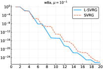
(a)

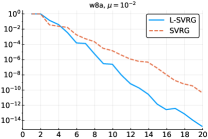
(b)

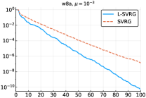
(c)

(d)

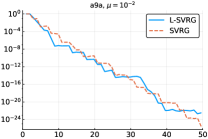
(e)

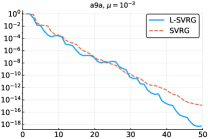
(f)

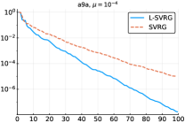
(g)

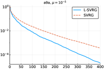
(h)

Figure 1: Comparison of SVRG and L-SVRG for different datasets and regularizer weights $\mu$.

Lemma 4.1.

We have

$$\begin{split}&{\rm E}\left[\left\lVert g^{k}-\nabla f(x^{k})\right\rVert^{2}\right]\leq 2L\left(f(w^{k})-f(x^{k})-\left<\nabla f(x^{k}),w^{k}-x^{k}\right>\right).\end{split}$$ (14)

Next two lemmas are more technical, but essential for proving the convergence.

Lemma 4.2.

We have

$$\begin{split}&\left<g^{k},x^{*}-z^{k+1}\right>+\tfrac{\mu}{2}\left\lVert x^{k}-x^{*}\right\rVert^{2}\geq\tfrac{L}{2\eta}\left\lVert z^{k}-z^{k+1}\right\rVert^{2}+{\cal Z}^{k+1}-\tfrac{1}{1+\eta\sigma}{\cal Z}^{k}.\end{split}$$ (15)

Lemma 4.3.

We have

$$\begin{split}&\tfrac{1}{\theta_{1}}\left(f(y^{k+1})-f(x^{k})\right)-\tfrac{\theta_{2}}{2L\theta_{1}}\left\lVert g^{k}-\nabla f(x^{k})\right\rVert^{2}\leq\tfrac{L}{2\eta}\left\lVert z^{k+1}-z^{k}\right\rVert^{2}+\left<g^{k},z^{k+1}-z^{k}\right>.\end{split}$$ (16)

Finally, we use the update of Algorithm 2 to decompose ${\cal W}^{k+1}$ in terms of ${\cal W}^{k}$ and ${\cal Y}^{k}$, which is one of the main components that allow for simpler analysis than the one of original Katyusha.

Lemma 4.4.

We have

$$\begin{split}{\rm E}\left[{\cal W}^{k+1}\right]=(1-p){\cal W}^{k}+\theta_{2}(1+\theta_{1}){\cal Y}^{k}.\end{split}$$ (17)

Putting all lemmas together, we obtain the following contraction of the Lyapunov function (7).

Lemma 4.5.

Let $\theta_{1},\theta_{2}>0$, $\theta_{1}+\theta_{2}\leq 1$, $\sigma=\frac{\mu}{L}$ and $\eta=\frac{\theta_{2}}{(1+\theta_{2})\theta_{1}}$, then we have

$$\begin{split}&{\rm E}\left[{\cal Z}^{k+1}+{\cal Y}^{k+1}+{\cal W}^{k+1}\right]\leq\tfrac{1}{1+\eta\sigma}{\cal Z}^{k}+(1-\theta_{1}(1-\theta_{2})){\cal Y}^{k}+\left(1-\tfrac{p\theta_{1}}{1+\theta_{1}}\right){\cal W}^{k}.\end{split}$$ (18)

In order to obtain a recursion involving the Lyapunov function on the right-hand side of (18)

Theorem 4.6.

Let $\theta_{1}=\min\{\sqrt{\nicefrac{{2\sigma n}}{{3}}},\nicefrac{{1}}{{2}}\}$, $\theta_{2}=\nicefrac{{1}}{{2}}$, $p=\nicefrac{{1}}{{n}}$. Then ${\rm E}\left[\Psi^{k}\right]\leq\varepsilon\Psi^{0}$ after the following number of iterations: $k={\cal O}((n+\sqrt{\nicefrac{{nL}}{{\mu}}})\log\nicefrac{{1}}{{\varepsilon}}).$

Proof.

From Lemma 4.5 we get ${\rm E}\left[\Psi^{k+1}\right]\leq\max\left\{\nicefrac{{1}}{{(1+\eta\sigma)}},1-\theta_{1}(1-\theta_{2}),1-\nicefrac{{p\theta_{1}}}{{(1+\theta_{1})}}\right\}\Psi^{k}.$ Setting $p=\nicefrac{{1}}{{n}}$, $\theta_{1}=\min\{\sqrt{\nicefrac{{2\sigma n}}{{3}}},\nicefrac{{1}}{{2}}\}$, $\theta_{2}=\nicefrac{{1}}{{2}}$, and unrolling conditional probability one obtains ${\rm E}\left[\Psi^{k+1}\right]\leq(1-\theta){\rm E}\left[\Psi^{k}\right]$, where $\theta=\min\left\{\nicefrac{{\sigma}}{{6\theta_{1}}},\nicefrac{{\theta_{1}}}{{2n}}\right\}.$ Choosing $\sigma=\nicefrac{{\mu}}{{L}}$ concludes the proof. ∎

Discussion. One can show by analyzing (18) that for ill-conditioned problems ($n<\nicefrac{{L}}{{\mu}}$), the iteration complexity is ${\cal O}(\sqrt{\nicefrac{{L}}{{\mu p}}}\log\nicefrac{{1}}{{\varepsilon}})$. Algorithm 2 calls stochastic gradient oracle ${\cal O}(1+pn)$ times per iteration in expectation. Thus, the total complexity is ${\cal O}((1+pn)\sqrt{\nicefrac{{L}}{{\mu p}}}\log\nicefrac{{1}}{{\varepsilon}})$. One can see that $p=\Theta\left(\nicefrac{{1}}{{n}}\right)$ leads to optimal rate.

5 Numerical Experiments

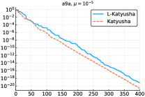
(a)

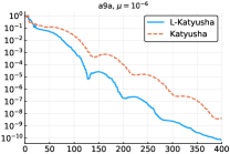
(b)

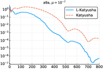
(c)

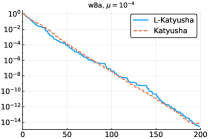
(d)

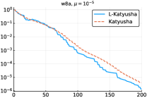
(e)

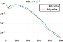
(f)

Figure 2: Comparison of Katyusha & L-Katyusha for different datasets and regularizer weights $\mu$.

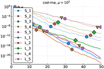
(a)

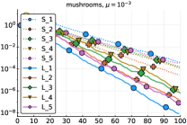
(b)

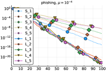
(c)

Figure 3: Comparison of SVRG (S) and L-SVRG (L) for several choices of expected outer loop length (L-SVRG) or deterministic outer loop length (SVRG). Numbers $1$–$5$ correspondent to loop-lengths $n$,$\sqrt[4]{\kappa n^{3}}$, $\sqrt{\kappa n}$, $\sqrt[4]{\kappa^{3}n}$, $\kappa$, respectively, where $\kappa=\nicefrac{{L}}{{\mu}}$.

In this section, we perform experiments with logistic regression for binary classification with $L_{2}$ regularizer, where our loss function has the form $f_{i}(x)=\log(1+\exp(-b_{i}a_{i}^{\top}x))+\tfrac{\mu}{2}\left\lVert x\right\rVert^{2},$ where $a_{i}\in\mathbb{R}^{d}$, $b_{i}\in\{-1,+1\}$, $i\in[n]$. Hence, $f$ is smooth and $\mu$-strongly convex. We use four LIBSVM library: a9a, w8a, mushrooms, phishing, cod-rna.

We compare our methods L-SVRG and L-Katyusha with their original version. It is well-known that whenever practical, SAGA is a bit faster than SVRG. While a comparison to SAGA seems natural as it also does not have a double loop structure, we position our loopless methods for applications where the high memory requirements of SAGA prevent it to be applied. Thus, we do not compare to SAGA.

Plots are constructed in such a way that the $y$-axis displays $\left\lVert x^{k}-x^{\star}\right\rVert^{2}$ for L-SVRG and $\left\lVert y^{k}-x^{\star}\right\rVert^{2}$ for L-Katyusha, where $x^{\star}$ were obtained by running gradient descent for a large number of epochs. The $x$-axis displays the number of epochs (full gradient evaluations). That is, $n$ computations of $\nabla f_{i}(x)$ equals one epoch.

Superior practical behaviour of the loopless approach. Here we show that L-SVRG and L-Katyusha perform better in experiments than their loopy variants. In terms of theoretical iteration complexity, both the loopy and the loopless methods are the same. However, as we can see from Figure 1, the improvement of the loopless approach can be significant. One can see that for these datasets, L-SVRG is always better than SVRG, and can be faster by several orders of magnitude! Looking at Figure 2, we see that the performance of L-Katyusha is at least as good as that of Katyusha, and can be significantly faster in some cases. All parameters of the methods were chosen as suggested by theory. For L-SVRG and L-Katyusha they are chosen based on Theorems 3.5 and 4.6, respectively. For SVRG and Katyusha we also choose the parameters based on the theory, as described in the original papers. The initial point $x^{0}$ is chosen to be the origin.

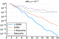
(a)

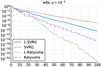
(b)

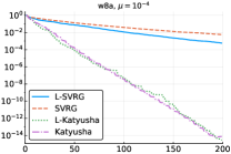
(c)

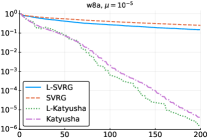
(d)

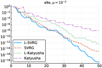
(e)

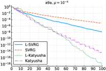
(f)

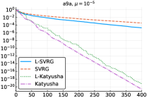
(g)

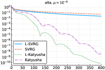
(h)

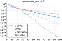
(i)

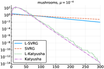
(j)

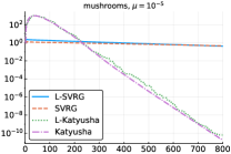
(k)

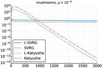
(l)

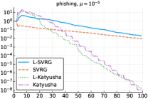
(m)

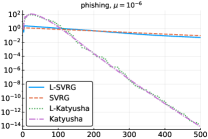
(n)

(o)

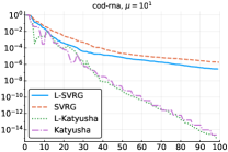
(p)

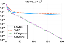
(q)

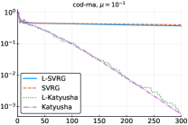
(r)

Figure 4: All methods together for different datasets and different regularizer weights.

Different choices of probability/ outer loop size. We now compare several choices of the probability $p$ of updating the full gradient for SVRG and several outer loop sizes $m$ for SVRG. Since our analysis guarantees the optimal rate for any choice of $p$ between $\nicefrac{{1}}{{n}}$ and $\nicefrac{{\mu}}{{L}}$ for well condition problems, we decided to perform experiments for $p$ within this range. More precisely, we choose $5$ values of $p$, uniformly distributed in logarithmic scale across this interval, and thus our choices are $n$,$\sqrt[4]{\kappa n^{3}}$, $\sqrt{\kappa n}$, $\sqrt[4]{\kappa^{3}n}$, and $\kappa$, where $\kappa=\nicefrac{{L}}{{\mu}}$, denoted in the figures by $1,2,3,4,5$, respectively. Since the expected “outer loop” length (length for which reference point stays the same) is $\nicefrac{{1}}{{p}}$, for SVRG we choose $m=\nicefrac{{1}}{{p}}$. Looking at Figure 3, one can see that L-SVRG is very robust to the choice of $p$ from the “optimal interval” predicted by our theory. Moreover, even the worst case for L-SVRG outperforms the best case for SVRG.

All methods together. Finally, we provide all algorithms together in one plot for different datasets with different regularizer weight, thus with different condition numbers, displayed in Figure 4. As for the previous experiments, loopless methods are not worse and sometimes significantly better.

Supplementary Material:
SVRG and Katyusha are Better Without the Outer Loop

Appendix A Auxiliary Lemmas

Lemma A.1.

For random vector $x\in\mathbb{R}^{d}$ and any $y\in\mathbb{R}^{d}$, the variance of $y$ can be decomposed as

$${\rm E}\left[\left\lVert x-{\rm E}\left[x\right]\right\rVert^{2}\right]={\rm E}\left[\left\lVert x-y\right\rVert^{2}\right]-{\rm E}\left[\left\lVert{\rm E}\left[x\right]-y\right\rVert^{2}\right]\,.$$ (19)

The next lemma is a consequence of Jensen’s inequality applied to $x\mapsto\|x\|^{2}$.

Lemma A.2.

For any vectors $a_{1},a_{2},\dots,a_{k}\in\mathbb{R}^{d}$, the following inequality holds:

$$\left\|\sum_{i=1}^{k}a_{i}\right\|^{2}\leq k\sum_{i=1}^{k}\left\lVert a_{i}\right\rVert^{2}\,.$$ (20)

Appendix B Proofs for Algorithm 1 (L-SVRG)

In all proofs below, we will for simplicity write $f^{*}\overset{\text{def}}{=}f(x^{*})$.

B.1 Proof of Lemma 3.1

Definition of $x^{k+1}$ and unbiasness of $g^{k}$ guarantee that

$${\rm E}\left[\left\lVert x^{k+1}-x^{*}\right\rVert^{2}\right] = {\rm E}\left[\left\lVert x^{k}-x^{*}-\eta g^{k}\right\rVert\right]^{2}$$

$$\overset{\text{Alg.}~{}\ref{alg:1}}{=} \left\lVert x^{k}-x^{*}\right\rVert^{2}+{\rm E}\left[2\eta\left<g^{k},x^{*}-x^{k}\right>\right]+\eta^{2}{\rm E}\left[\left\lVert g^{k}\right\rVert^{2}\right]$$

$$\overset{\eqref{eq:unbiased}}{=} \left\lVert x^{k}-x^{*}\right\rVert^{2}+2\eta\left<\nabla f(x^{k}),x^{*}-x^{k}\right>+\eta^{2}{\rm E}\left[\left\lVert g^{k}\right\rVert^{2}\right]$$

$$\overset{\eqref{def:strong_convexity}}{\leq} \left\lVert x^{k}-x^{*}\right\rVert^{2}+2\eta\left(f^{*}-f(x^{k})-\frac{\mu}{2}\left\lVert x^{k}-x^{*}\right\rVert\right)+\eta^{2}{\rm E}\left[\left\lVert g^{k}\right\rVert^{2}\right]$$

$$= \left\lVert x^{k}-x^{*}\right\rVert^{2}(1-\eta\mu)+2\eta\left(f^{*}-f(x^{k})\right)+\eta^{2}{\rm E}\left[\left\lVert g^{k}\right\rVert^{2}\right].$$

B.2 Proof of Lemma 3.2

Using definition of $g^{k}$

$${\rm E}\left[\left\lVert g^{k}\right\rVert^{2}\right] \overset{\text{Alg.}~{}\ref{alg:1}}{=} {\rm E}\left[\left\lVert\nabla f_{i}(x^{k})-\nabla f_{i}(x^{*})+\nabla f_{i}(x^{*})-\nabla f_{i}(w^{k})+\nabla f(w^{k})\right\rVert^{2}\right]$$

$$\overset{\eqref{eq:sum}}{\leq} 2{\rm E}\left[\left\lVert\nabla f_{i}(x^{k})-\nabla f_{i}(x^{*})\right\rVert^{2}\right]+2{\rm E}\left[\left\lVert\nabla f_{i}(x^{*})-\nabla f_{i}(w^{k})-{\rm E}\left[\nabla f_{i}(x^{*})-\nabla f_{i}(w^{k})\right]\right\rVert^{2}\right]$$

$$\overset{\eqref{def:L-smoothness}+\eqref{eq:variance}}{\leq} 4L(f(x^{k})-f^{*})+2{\rm E}\left[\left\lVert\nabla f_{i}(w^{k})-\nabla f_{i}(x^{*})\right\rVert^{2}\right]$$

$$\overset{\eqref{def:D^k_alg_1}}{=} 4L(f(x^{k})-f^{*})+\frac{p}{2\eta^{2}}{\cal D}^{k}.$$

B.3 Proof of Lemma 3.3

$${\rm E}\left[{\cal D}^{k+1}\right] \overset{\text{Alg.}~{}\ref{alg:1}}{=} (1-p){\cal D}^{k}+p\frac{4\eta^{2}}{pn}\sum\limits_{i=1}^{n}\left\lVert\nabla f(x^{k})-\nabla f(x^{*})\right\rVert^{2}$$

$$\overset{\eqref{def:L-smoothness}}{\leq} (1-p){\cal D}^{k}+8L\eta^{2}(f(x^{k})-f^{*}).$$

B.4 Proof of Lemma 3.4

Combining Lemmas 3.1 and 3.3 we obtain

$${\rm E}\left[\left\lVert x^{k+1}-x^{*}\right\rVert^{2}+{\cal D}^{k+1}\right] \overset{\eqref{eq:x^k_alg_1}+\eqref{eq:D^k_alg_1}}{\leq} (1-\mu\eta)\left\lVert x^{k}-x^{*}\right\rVert^{2}+2\eta(f^{*}-f(x^{k}))+\eta^{2}{\rm E}\left[\left\lVert g^{k}\right\rVert^{2}\right]$$

$$\quad+(1-p){\cal D}^{k}+8L\eta^{2}(f(x^{k})-f^{*})$$

$$\overset{\eqref{eq:g^k_alg_1}}{\leq} (1-\mu\eta)\left\lVert x^{k}-x^{*}\right\rVert^{2}+(1-p){\cal D}^{k}+(2\eta-8L\eta^{2})(f^{*}-f(x^{k}))$$

$$\quad+\eta^{2}\left(4L(f(x^{k})-f^{*})+\frac{p}{2\eta^{2}}{\cal D}^{k}\right)$$

$$= (1-\mu\eta)\left\lVert x^{k}-x^{*}\right\rVert^{2}+\left(1-\frac{p}{2}\right){\cal D}^{k}+(2\eta-12L\eta^{2})(f^{*}-f(x^{k})).$$

Now we use the fact that $\eta\leq\frac{1}{6L}$ and obtain the desired inequality:

$${\rm E}\left[\left\lVert x^{k+1}-x^{*}\right\rVert^{2}+{\cal D}^{k+1}\right] \leq (1-\mu\eta)\left\lVert x^{k}-x^{*}\right\rVert^{2}+\left(1-\frac{p}{2}\right){\cal D}^{k}.$$

Appendix C Proofs for Algorithm 2 (L-Katyusha)

C.1 Proof of Lemma 4.1

To upper bound the variance of $g^{k}$ we first uses its definition

$${\rm E}\left[\left\lVert g^{k}-\nabla f(x^{k})\right\rVert^{2}\right] \overset{\text{Alg.}~{}\ref{alg:2}}{=} {\rm E}\left[\left\lVert\nabla f_{i}(x^{k})-\nabla f_{i}(w^{k})-{\rm E}\left[\nabla f_{i}(x^{k})-\nabla f_{i}(w^{k})\right]\right\rVert^{2}\right]$$

$$\overset{\eqref{eq:variance}}{\leq} {\rm E}\left[\left\lVert\nabla f_{i}(x^{k})-\nabla f_{i}(w^{k})\right\rVert^{2}\right]$$

$$\overset{\eqref{def:L-smoothness}}{\leq} 2L\left(f(w^{k})-f(x^{k})-\left<\nabla f(x^{k}),w^{k}-x^{k}\right>\right).$$

C.2 Proof of Lemma 4.2

We start with the definition of $z^{k+1}$

$$z^{k+1}\overset{\text{Alg.}~{}\ref{alg:2}}{=}\frac{1}{1+\eta\sigma}\left(\eta\sigma x^{k}+z^{k}-\frac{\eta}{L}g^{k}\right),$$

which implies $\frac{\eta}{L}g^{k}=\eta\sigma(x^{k}-z^{k+1})+(z^{k}-z^{k+1}),$ which further implies that

$$\left<g^{k},z^{k+1}-x^{*}\right> = \mu\left<x^{k}-z^{k+1},z^{k+1}-x^{*}\right>+\frac{L}{\eta}\left<z^{k}-z^{k+1},z^{k+1}-x^{*}\right>$$

$$= \frac{\mu}{2}\left(\left\lVert x^{k}-x^{*}\right\rVert^{2}-\left\lVert x^{k}-z^{k+1}\right\rVert^{2}-\left\lVert z^{k+1}-x^{*}\right\rVert^{2}\right)$$

$$\quad+\frac{L}{2\eta}\left(\left\lVert z^{k}-x^{*}\right\rVert^{2}-\left\lVert z^{k}-z^{k+1}\right\rVert^{2}-\left\lVert z^{k+1}-x^{*}\right\rVert^{2}\right)$$

$$\leq \frac{\mu}{2}\left\lVert x^{k}-x^{*}\right\rVert^{2}+\frac{L}{2\eta}\left(\left\lVert z^{k}-x^{*}\right\rVert^{2}-(1+\eta\sigma)\left\lVert z^{k+1}-x^{*}\right\rVert^{2}\right)-\frac{L}{2\eta}\left\lVert z^{k}-z^{k+1}\right\rVert^{2}.$$

C.3 Proof of Lemma 4.3

$$\frac{L}{2\eta}\left\lVert z^{k+1}-z^{k}\right\rVert^{2}+\left<g^{k},z^{k+1}-z^{k}\right>$$

$$= \frac{1}{\theta_{1}}\left(\frac{L}{2\eta\theta_{1}}\left\lVert\theta_{1}(z^{k+1}-z^{k})\right\rVert^{2}+\left<g^{k},\theta_{1}(z^{k+1}-z^{k})\right>\right)$$

$$\overset{\text{Alg.}~{}\ref{alg:2}}{=} \frac{1}{\theta_{1}}\left(\frac{L}{2\eta\theta_{1}}\left\lVert y^{k+1}-x^{k}\right\rVert^{2}+\left<g^{k},y^{k+1}-x^{k}\right>\right)$$

$$= \frac{1}{\theta_{1}}\left(\frac{L}{2\eta\theta_{1}}\left\lVert y^{k+1}-x^{k}\right\rVert^{2}+\left<\nabla f(x^{k}),y^{k+1}-x^{k}\right>+\left<g^{k}-\nabla f(x^{k}),y^{k+1}-x^{k}\right>\right)$$

$$= \frac{1}{\theta_{1}}\left(\frac{L}{2}\left\lVert y^{k+1}-x^{k}\right\rVert^{2}+\left<\nabla f(x^{k}),y^{k+1}-x^{k}\right>+\frac{L}{2}\left(\frac{1}{\eta\theta_{1}}-1\right)\left\lVert y^{k+1}-x^{k}\right\rVert^{2}+\left<g^{k}-\nabla f(x^{k}),y^{k+1}-x^{k}\right>\right)$$

$$\overset{\eqref{def:L-smoothness}}{\geq} \frac{1}{\theta_{1}}\left(f(y^{k+1})-f(x^{k})+\frac{L}{2}\left(\frac{1}{\eta\theta_{1}}-1\right)\left\lVert y^{k+1}-x^{k}\right\rVert^{2}+\left<g^{k}-\nabla f(x^{k}),y^{k+1}-x^{k}\right>\right)$$

$$\geq \frac{1}{\theta_{1}}\left(f(y^{k+1})-f(x^{k})-\frac{\eta\theta_{1}}{2L(1-\eta\theta_{1})}\left\lVert g^{k}-\nabla f(x^{k})\right\rVert^{2}\right)$$

$$= \frac{1}{\theta_{1}}\left(f(y^{k+1})-f(x^{k})-\frac{\theta_{2}}{2L}\left\lVert g^{k}-\nabla f(x^{k})\right\rVert^{2}\right),$$

where the last inequality uses the Young’s inequality in the form of $\left<a,b\right>\geq-\frac{\left\lVert a\right\rVert^{2}}{2\beta}-\frac{\beta\left\lVert b\right\rVert^{2}}{2}$ for $\beta=\frac{\eta\theta_{1}}{L(1-\eta\theta_{1})}$, which concludes the proof.

C.4 Proof of Lemma 4.4

From the definition of $w^{k+1}$ in Algorithm 2 we have

$${\rm E}\left[f(w^{k+1})\right]\overset{\text{Alg.}~{}\ref{alg:2}}{=}(1-p)f(w^{k})+pf(y^{k}).$$ (21)

The rest of proof follows from the definition of ${\cal W}^{k}$ (17).

C.5 Proof of Lemma 4.5

Combining all the previous lemmas together, we obtain

$$f^{*} \overset{\eqref{def:strong_convexity}}{\geq} f(x^{k})+\left<\nabla f(x^{k}),x^{*}-x^{k}\right>+\frac{\mu}{2}\left\lVert x^{k}-x^{*}\right\rVert^{2}$$

$$= f(x^{k})+\frac{\mu}{2}\left\lVert x^{k}-x^{*}\right\rVert^{2}+\left<\nabla f(x^{k}),x^{*}-z^{k}+z^{k}-x^{k}\right>$$

$$\overset{\text{Alg.}~{}\ref{alg:2}}{=} f(x^{k})+\frac{\mu}{2}\left\lVert x^{k}-x^{*}\right\rVert^{2}+\left<\nabla f(x^{k}),x^{*}-z^{k}\right>+\frac{\theta_{2}}{\theta_{1}}\left<\nabla f(x^{k}),x^{k}-w^{k}\right>+\frac{(1-\theta_{1}-\theta_{2})}{\theta_{1}}\left<\nabla f(x^{k}),x^{k}-y^{k}\right>$$

$$\overset{\eqref{eq:unbiased}}{\geq} f(x^{k})+\frac{\theta_{2}}{\theta_{1}}\left<\nabla f(x^{k}),x^{k}-w^{k}\right>+\frac{(1-\theta_{1}-\theta_{2})}{\theta_{1}}(f(x^{k})-f(y^{k}))$$

$$\quad+{\rm E}\left[\frac{\mu}{2}\left\lVert x^{k}-x^{*}\right\rVert^{2}+\left<g^{k},x^{*}-z^{k+1}\right>+\left<g^{k},z^{k+1}-z^{k}\right>\right]$$

$$\overset{\eqref{eq:wg_alg_2}}{\geq} f(x^{k})+\frac{\theta_{2}}{\theta_{1}}\left<\nabla f(x^{k}),x^{k}-w^{k}\right>+\frac{(1-\theta_{1}-\theta_{2})}{\theta_{1}}(f(x^{k})-f(y^{k}))$$

$$\quad+{\rm E}\left[{\cal Z}^{k+1}-\frac{1}{1+\eta\sigma}{\cal Z}^{k}\right]+{\rm E}\left[\left<g^{k},z^{k+1}-z^{k}\right>+\frac{L}{2\eta}\left\lVert z^{k}-z^{k+1}\right\rVert^{2}\right]$$

$$\overset{\eqref{eq:wtheta_alg_2}}{\geq} f(x^{k})+\frac{\theta_{2}}{\theta_{1}}\left<\nabla f(x^{k}),x^{k}-w^{k}\right>+\frac{(1-\theta_{1}-\theta_{2})}{\theta_{1}}(f(x^{k})-f(y^{k}))$$

$$\quad+{\rm E}\left[{\cal Z}^{k+1}-\frac{1}{1+\eta\sigma}{\cal Z}^{k}\right]+{\rm E}\left[\frac{1}{\theta_{1}}\left(f(y^{k+1})-f(x^{k})\right)-\frac{\theta_{2}}{2L\theta_{1}}\left\lVert g^{k}-\nabla f(x^{k})\right\rVert^{2}\right]$$

$$\overset{\eqref{eq:g^k_alg_2}}{\geq} f(x^{k})+\frac{\theta_{2}}{\theta_{1}}\left<\nabla f(x^{k}),x^{k}-w^{k}\right>+\frac{(1-\theta_{1}-\theta_{2})}{\theta_{1}}(f(x^{k})-f(y^{k}))$$

$$\quad+{\rm E}\left[{\cal Z}^{k+1}-\frac{1}{1+\eta\sigma}{\cal Z}^{k}\right]+{\rm E}\left[\frac{1}{\theta_{1}}\left(f(y^{k+1})-f(x^{k})\right)-\frac{\theta_{2}}{\theta_{1}}\left(f(w^{k})-f(x^{k})-\left<\nabla f(x^{k}),w^{k}-x^{k}\right>\right)\right]$$

$$= f(x^{k})+\frac{(1-\theta_{1}-\theta_{2})}{\theta_{1}}(f(x^{k})-f(y^{k}))-\frac{1}{1+\eta\sigma}{\cal Z}^{k}-\frac{\theta_{2}}{\theta_{1}}(f(w^{k})-f(x^{k}))$$

$$\quad+{\rm E}\left[{\cal Z}^{k+1}+\frac{1}{\theta_{1}}\left(f(y^{k+1})-f(x^{k})\right)\right],$$

where in the second inequality we use also convexity of $f(x)$.

$$x^{k} \overset{\text{Alg.}~{}\ref{alg:2}}{=} \theta_{1}z^{k}+\theta_{2}w^{k}+(1-\theta_{1}-\theta_{2})y^{k}$$

$$z^{k}-x^{k} = \frac{\theta_{2}}{\theta_{1}}(x^{k}-w^{k})+\frac{1-\theta_{1}-\theta_{2}}{\theta_{1}}(x^{k}-y^{k}).$$

After rearranging we get

$$\frac{1}{1+\eta\sigma}{\cal Z}^{k}+(1-\theta_{1}-\theta_{2}){\cal Y}^{k}+\frac{\theta_{2}}{\theta_{1}}(f(w^{k}-f^{*}))\geq{\rm E}\left[{\cal Z}^{k+1}+{\cal Y}^{k+1}\right].$$

Using definition of ${\cal W}^{k}$ we get

$${\rm E}\left[{\cal Z}^{k+1}+{\cal Y}^{k+1}\right]\leq\frac{1}{1+\eta\sigma}{\cal Z}^{k}+(1-\theta_{1}-\theta_{2}){\cal Y}^{k}+\frac{p}{(1+\theta_{1})}{\cal W}^{k}.$$ (22)

Finally, using Lemma 4.4 we get

$${\rm E}\left[{\cal Z}^{k+1}+{\cal Y}^{k+1}+{\cal W}^{k+1}\right] \leq \frac{1}{1+\eta\sigma}{\cal Z}^{k}+(1-\theta_{1}-\theta_{2}){\cal Y}^{k}+\frac{p}{(1+\theta_{1})}{\cal W}^{k}+(1-p){\cal W}^{k}+\theta_{2}(1+\theta_{1}){\cal Y}^{k}$$

$$= \frac{1}{1+\eta\sigma}{\cal Z}^{k}+(1-\theta_{1}(1-\theta_{2})){\cal Y}^{k}+\left(1-\frac{p\theta_{1}}{1+\theta_{1}}\right){\cal W}^{k},$$

which concludes the proof.

References

- [1] Zeyuan Allen-Zhu. Katyusha: The first direct acceleration of stochastic gradient methods. In Proceedings of the 49th Annual ACM SIGACT Symposium on Theory of Computing, pages 1200–1205. ACM, 2017.
- [2] Adel Bibi, Alibek Sailanbayev, Bernard Ghanem, Robert Mansel Gower, and Peter Richtárik. Improving SAGA via a probabilistic interpolation with gradient descent. arXiv: 1806.05633, 2018.
- [3] Dominik Csiba, Zheng Qu, and Peter Richtárik. Stochastic dual coordinate ascent with adaptive probabilities. In Proceedings of the 32nd International Conference on Machine Learning, pages 674–683, 2015.
- [4] Dominik Csiba and Peter Richtárik. Primal method for ERM with flexible mini-batching schemes and non-convex losses. arXiv:1506.02227, 2015.
- [5] Aaron Defazio. A simple practical accelerated method for finite sums. In Advances in Neural Information Processing Systems, pages 676–684, 2016.
- [6] Aaron Defazio, Francis Bach, and Simon Lacoste-Julien. SAGA: A fast incremental gradient method with support for non-strongly convex composite objectives. In Advances in Neural Information Processing Systems, pages 1646–1654, 2014.
- [7] Aaron Defazio, Tiberio Caetano, and Justin Domke. Finito: A faster, permutable incremental gradient method for Big Data problems. The 31st International Conference on Machine Learning, 2014.
- [8] Nikita Doikov and Peter Richtárik. Randomized block cubic Newton method. In Proceedings of the 35th International Conference on Machine Learning, 2018.
- [9] Robert Mansel Gower, Donald Goldfarb, and Peter Richtárik. Stochastic block BFGS: squeezing more curvature out of data. In 33rd International Conference on Machine Learning, pages 1869–1878, 2016.
- [10] Robert Mansel Gower, Peter Richtárik, and Francis Bach. Stochastic quasi-gradient methods: variance reduction via Jacobian sketching. arXiv:1805.02632, 2018.
- [11] Thomas Hofmann, Aurelien Lucchi, Simon Lacoste-Julien, and Brian McWilliams. Variance reduced stochastic gradient descent with neighbors. In Advances in Neural Information Processing Systems, pages 2305–2313, 2015.
- [12] Rie Johnson and Tong Zhang. Accelerating stochastic gradient descent using predictive variance reduction. In Advances in Neural Information Processing Systems, pages 315–323, 2013.
- [13] Jakub Konečný, Jie Lu, Peter Richtárik, and Martin Takáč. Mini-batch semi-stochastic gradient descent in the proximal setting. IEEE Journal of Selected Topics in Signal Processing, 10(2):242–255, 2016.
- [14] Jakub Konečný and Peter Richtárik. S2GD: Semi-stochastic gradient descent methods. Frontiers in Applied Mathematics and Statistics, pages 1–14, 2017.
- [15] Lihua Lei, Cheng Ju, Jianbo Chen, and Michael I Jordan. Non-convex finite-sum optimization via CSSG methods. In Advances in Neural Information Processing Systems, pages 2348–2358, 2017.
- [16] Julien Mairal. Incremental majorization-minimization optimization with application to large-scale machine learning. SIAM Journal on Optimization, 25(2):829–855, 2015.
- [17] A Nemirovski, A Juditsky, G Lan, and A Shapiro. Robust stochastic approximation approach to stochastic programming. SIAM Journal on Optimization, 19(4):1574–1609, 2009.
- [18] Arkadi Nemirovsky and David B. Yudin. Problem complexity and method efficiency in optimization. Wiley, New York, 1983.
- [19] Yurii Nesterov. Introductory lectures on convex optimization: A basic course, volume 87. Springer Science & Business Media, 2013.
- [20] Lam M Nguyen, Jie Liu, Katya Scheinberg, and Martin Takáč. SARAH: A novel method for machine learning problems using stochastic recursive gradient. In International Conference on Machine Learning, pages 2613–2621, 2017.
- [21] Zheng Qu, Peter Richtárik, Martin Takáč, and Olivier Fercoq. SDNA: Stochastic dual Newton ascent for empirical risk minimization. In The 33rd International Conference on Machine Learning, pages 1823–1832, 2016.
- [22] Zheng Qu, Peter Richtárik, and Tong Zhang. Quartz: Randomized dual coordinate ascent with arbitrary sampling. In Advances in Neural Information Processing Systems 28, pages 865–873, 2015.
- [23] Nicolas Le Roux, Mark Schmidt, and Francis Bach. A stochastic gradient method with an exponential convergence rate for finite training sets. In Advances in Neural Information Processing Systems, pages 2663–2671, 2012.
- [24] Mark Schmidt, Nicolas Le Roux, and Francis Bach. Minimizing finite sums with the stochastic average gradient. Mathematical Programming, 162(1-2):83–112, 2017.
- [25] Shai Shalev-Shwartz. SDCA without duality, regularization, and individual convexity. In International Conference on Machine Learning, pages 747–754, 2016.
- [26] Shai Shalev-Shwartz and Tong Zhang. Accelerated proximal stochastic dual coordinate ascent for regularized loss minimization. In International Conference on Machine Learning, pages 64–72, 2014.
- [27] Martin Takáč, Avleen Bijral, Peter Richtárik, and Nathan Srebro. Mini-batch primal and dual methods for SVMs. In 30th International Conference on Machine Learning, pages 537–552, 2013.
- [28] Kaiwen Zhou. Direct acceleration of SAGA using sampled negative momentum. arXiv preprint arXiv:1806.11048, 2018.
- [29] Kaiwen Zhou, Fanhua Shang, and James Cheng. A simple stochastic variance reduced algorithm with fast convergence rates. arXiv preprint arXiv:1806.11027, 2018.