Abstract

We study the problem of minimizing the average of a very large number of smooth functions, which is of key importance in training supervised learning models. One of the most celebrated methods in this context is the SAGA algorithm of Defazio et al. (2014). Despite years of research on the topic, a general-purpose version of SAGA—one that would include arbitrary importance sampling and minibatching schemes—does not exist. We remedy this situation and propose a general and flexible variant of SAGA following the arbitrary sampling paradigm. We perform an iteration complexity analysis of the method, largely possible due to the construction of new stochastic Lyapunov functions. We establish linear convergence rates in the smooth and strongly convex regime, and under a quadratic functional growth condition (i.e., in a regime not assuming strong convexity). Our rates match those of the primal-dual method Quartz Qu et al. (2015) for which an arbitrary sampling analysis is available, which makes a significant step towards closing the gap in our understanding of complexity of primal and dual methods for finite sum problems.

1 Introduction

We consider a convex composite optimization problem

$$\textstyle\min_{x\in\mathbb{R}^{d}}P(x)\;{:=}\;\left(\sum\limits_{i=1}^{n}\lambda_{i}f_{i}(x)\right)+\psi(x),$$ (1)

where $f:=\sum_{i}\lambda_{i}f_{i}$ is a conic combination (with coefficients $\lambda_{1},\dots,\lambda_{n}>0$) of a very large number of smooth convex functions $f_{i}:\mathbb{R}^{d}\to\mathbb{R}$, and $\psi:\mathbb{R}^{d}\to\mathbb{R}\cup\{+\infty\}$ is a proper closed convex function. We do not assume $\psi$ to be smooth. In particular, $\psi$ can be the indicator function of a nonempty closed convex set, turning problem (1) into a constrained minimization of function $f$. We are interested in the regime where $n\gg d$, although all our theoretical results hold without this assumption.

In a typical setup in the literature, $\lambda_{i}=1/n$ for all $i\in[n]\;{:=}\;\{1,2,\dots,n\}$, $f_{i}(x)$ corresponds to the loss of a supervised machine learning model $x$ on example $i$ from a training dataset of size $n$, and $f$ represents the average loss (i.e., empirical risk). Problems of the form (1) are often called “finite-sum” or regularized empirical risk minimization (ERM) problems, and are of immense importance in supervised learning, essentially forming the dominant training paradigm Shalev-Shwartz & Ben-David (2014).

1.1 Variance-reduced methods

One of the most successful methods for solving ERM problems is stochastic gradient descent (SGD) Robbins & Monro (1951); Nemirovski et al. (2009) and its many variants, including those with minibatches Takáč et al. (2013), importance sampling Needell et al. (2015); Zhao & Zhang (2015) and momentum Loizou & Richtárik (2017a; b).

One of the most interesting developments in recent years concerns variance-reduced variants of SGD. The first method in this category is the celebrated stochastic average gradient (SAG) method of Schmidt et al. (2017). Many additional variance-reduced methods were proposed since, including SDCA Richtárik & Takáč (2014); Shalev-Shwartz & Zhang (2013); Shalev-Shwartz (2016), SAGA Defazio et al. (2014), SVRG Johnson & Zhang (2013); Xiao & Zhang (2014b), S2GD Konečný & Richtárik (2017); Konečný et al. (2016), MISO Mairal (2015), JacSketch Gower et al. (2018) and SAGD Bibi et al. (2018).

1.2 SAGA: the known and the unknown

Since the SAG gradient estimator is not unbiased, SAG is notoriously hard to analyze. Soon after SAG was proposed, the SAGA method Defazio et al. (2014) was developed, obtained by replacing the biased SAG estimator by a similar, but unbiased, SAGA estimator. This method admits a simpler analysis, retaining the favourable convergence properties of SAG. SAGA is one of the early and most successful variance-reduced methods for (1).

Better understanding of the behaviour of SAGA remains one of the open challenges in the literature. Consider problem (1) with $\lambda_{i}=1/n$ for all $i$. Assume, for simplicity, that each $f_{i}$ is $L_{i}$-smooth and $f$ is $\mu$-strongly convex. In this regime, the iteration complexity of SAGA with uniform sampling probabilities is ${\cal O}((n+\tfrac{L_{\max}}{\mu})\log\tfrac{1}{\epsilon})$, where $L_{\max}\;{:=}\;\max_{i}L_{i}$, which was established already by Defazio et al. (2014). Schmidt et al. (2015) conjectured that there exist nonuniform sampling probabilities for which the complexity improves to ${\cal O}((n+\tfrac{\bar{L}}{\mu})\log\tfrac{1}{\epsilon})$, where ${\bar{L}}\;{:=}\;\sum_{i}L_{i}/n$. However, the “correct” importance sampling strategy leading to this result was not discovered until recently in the work of Gower et al. (2018), where the conjecture was resolved in the affirmative. One of the key difficulties in the analysis was the construction of a suitable stochastic Lyapunov function controlling the iterative process. Likewise, until recently, very little was known about the minibatch performance of SAGA, even for the simplest uniform minibatch strategies. Notable advancements in this area were made by Gower et al. (2018), who have the currently best rates for SAGA with standard uniform minibatch strategies and the first importance sampling results for a block variant of SAGA.

1.3 Contributions

Regime	Arbitrary sampling	Theorem
Smooth $\psi\equiv 0$ $f_{i}$ is $L_{i}$-smooth, $f$ is $\mu$-strongly convex	$\displaystyle\max_{1\leq i\leq n}\left\{\tfrac{1}{{\color[rgb]{1,0,0}p_{i}}}+\tfrac{4L_{i}{\color[rgb]{0,0,1}\beta_{i}}\lambda_{i}}{\mu}\right\}\log\left(\tfrac{1}{\epsilon}\right)$	3.1
Nonsmooth $P$ satisfies $\mu$-growth condition (19) and Assumption 4.3 $f_{i}(x)=\phi_{i}({\bf A}_{i}^{\top}x)$, $\phi_{i}$ is $1/\gamma$-smooth, $f$ is $L$-smooth	$\displaystyle\left(2+\max\left\{\tfrac{6L}{\mu},3\max_{1\leq i\leq n}\left\{\tfrac{1}{{\color[rgb]{1,0,0}p_{i}}}+\tfrac{4{\color[rgb]{0,0,1}v_{i}}\lambda_{i}}{{\color[rgb]{1,0,0}p_{i}}\mu\gamma}\right\}\right\}\right)\log\left(\tfrac{1}{\epsilon}\right)$	4.4
Nonsmooth $\psi$ is $\mu$-strongly convex $f_{i}(x)=\phi_{i}({\bf A}_{i}^{\top}x)$, $\phi_{i}$ is $1/\gamma$-smooth	$\displaystyle\max_{1\leq i\leq n}\left\{1+\tfrac{1}{{\color[rgb]{1,0,0}p_{i}}}+\tfrac{3{\color[rgb]{0,0,1}v_{i}}\lambda_{i}}{{\color[rgb]{1,0,0}p_{i}}\mu\gamma}\right\}\log\left(\tfrac{1}{\epsilon}\right)$	4.6

Table 1: Iteration complexity results for SAGA-AS. We have ${\color[rgb]{1,0,0}p_{i}}\;{:=}\;\mathbb{P}(i\in S)$, where $S$ is a sampling of subsets of $[n]$ utilized by SAGA-AS. The key complexity parameters $\color[rgb]{0,0,1}\beta_{i}$ and $\color[rgb]{0,0,1}v_{i}$ are defined in the sections containing the theorems.

Our contributions can be summarized as follows.

SAGA with arbitrary sampling. We study the performance of SAGA under fully general data sampling strategies known in the literature as arbitrary sampling, generalizing all previous results, and obtaining an array of new theoretically and practically useful samplings. We call our general method SAGA-AS. Our theorems are expressed in terms of new stochastic and deterministic Lyapunov functions, the constructions of which was essential to our success.

In the arbitrary sampling paradigm, first proposed by Richtárik & Takáč (2016) in the context of randomized coordinate descent methods, one considers all (proper) random set valued mappings $S$ (called “samplings”) with values being subsets of $[n]$. A sampling is uniquely determined by assigning a probability to all $2^{n}$ subsets of $[n]$. A sampling is called proper if probability of each $i\in[n]$ being sampled is positive; that is, if $p_{i}\;{:=}\;\mathbb{P}(i\in S)>0$ for all $i$. Finally, the term “arbitrary sampling” refers to an arbitrary proper sampling.

Smooth case. We perform an iteration complexity analysis in the smooth case ($\psi\equiv 0$), assuming $f$ is $\mu$-strongly convex. Our analysis generalizes the results of Defazio et al. (2014) and Gower et al. (2018) to arbitrary sampling. The JacSketch method Gower et al. (2018) and its analysis rely on the notion of a bias-correcting random variable. Unfortunately, such a random variable does not exist for SAGA-AS. We overcome this obstacle by proposing a bias-correcting random vector (BCRV) which, as we show, always exists. While Gower et al. (2018); Bibi et al. (2018) consider particular suboptimal choices, we are able to find the BCRV which minimizes the iteration complexity bound. Unlike all known and new variants of SAGA considered in Gower et al. (2018), SAGA-AS does not arise as a special case of JacSketch. Our linear rates for SAGA-AS are the same as those for the primal-dual stochastic fixed point method Quartz Qu et al. (2015) (the first arbitrary sampling based method for (1)) in the regime when Quartz is applicable, which is the case when an explicit strongly convex regularizer is present. In contrast, we do not need an explicit regularizer, which means that SAGA-AS can utilize the strong convexity of $f$ fully, even if the strong convexity parameter $\mu$ is not known. While the importance sampling results in Gower et al. (2018) require each $f_{i}$ to be strongly convex, we impose this requirement on $f$ only.

Nonsmooth case. We perform an iteration complexity analysis in the general nonsmooth case. When the regularizer $\psi$ is strongly convex, which is the same setting as that considered in Qu et al. (2015), our iteration complexity bounds are essentially the same as that of Quartz. However, we also prove linear convergence results, with the same rates, under a quadratic functional growth condition (which does not imply strong convexity) Necoara et al. (2018). These are the first linear convergence result for any variant of SAGA without strong convexity. Moreover, to the best of our knowledge, SAGA-AS is the only variance-reduced method which achieves linear convergence without any a priori knowledge of the error bound condition number.

Our arbitrary sampling rates are summarized in Table 1.

1.4 Brief review of arbitrary sampling results

The arbitrary sampling paradigm was proposed by Richtárik & Takáč (2016), where a randomized coordinate descent method with arbitrary sampling of subsets of coordinates was analyzed for unconstrained minimization of a strongly convex function. Subsequently, the primal-dual method Quartz with arbitrary sampling of dual variables was studied in Qu et al. (2015) for solving (1) in the case when $\psi$ is strongly convex (and $\lambda_{i}=\tfrac{1}{n}$ for all $i$). An accelerated randomized coordinate descent method with arbitrary sampling called ALPHA was proposed by Qu & Richtárik (2016a) in the context of minimizing the sum of a smooth convex function and a convex block-separable regularizer. A key concept in the analysis of all known methods in the arbitrary sampling paradigm is the notion of expected separable overapproximation (ESO), introduced by Richtárik & Takáč (2016), and in the context of arbitrary sampling studied in depth by Qu & Richtárik (2016b). A stochastic primal-dual hybrid gradient algorithm (aka Chambolle-Pock) with arbitrary sampling of dual variables was studied by Chambolle et al. (2017). Recently, an accelerated coordinate descent method with arbitrary sampling for minimizing a smooth and strongly convex function was studied by Hanzely & Richtárik (2018). Finally, the first arbitrary sampling analysis in a nonconvex setting was performed by Horváth & Richtárik (2018), which is also the first work in which the optimal sampling out of class of all samplings of a given minibatch size was identified.

2 The Algorithm

Let $F:\mathbb{R}^{d}\to\mathbb{R}^{n}$ be defined by

$$\textstyle F(x)\;{:=}\;(f_{1}(x),...,f_{n}(x))^{\top}$$

and let ${\bf G}(x)\;{:=}\;[\nabla f_{1}(x),...,\nabla f_{n}(x)]\in{\mathbb{R}^{d\times n}}$ be the Jacobian of $F$ at $x$.

2.1 JacSketch

Gower et al. (2018) propose a new family of variance reduced SGD methods—called JacSketch—which progressively build a variance-reduced estimator of the gradient via the utilization of a new technique they call Jacobian sketching. As shown in Gower et al. (2018), state-of-the-art variants SAGA can be obtained as a special case of JacSketch. However, SAGA-AS does not arise as a special case of JacSketch. In fact, the generic analysis provided in Gower et al. (2018) (Theorem 3.6) is too coarse and does not lead to good bounds for any variants of SAGA with importance sampling. On the other hand, the analysis of Gower et al. (2018) which does do well for importance sampling does not generalize to arbitrary sampling, regularized objectives or regimes without strong convexity.

In this section we provide a brief review of the JacSketch method, establishing some useful notation along the way, with the goal of pointing out the moment of departure from JacSketch construction which leads to SAGA-AS. The iterations of JacSketch have the form

$$x^{k+1}=x^{k}-\alpha g^{k},$$ (2)

where $\alpha>0$ is a fixed step size, and $g^{k}$ is an variance-reduced unbiased estimator of the gradient $\nabla f(x^{k})$ built iteratively through a process involving Jacobian sketching, sketch-and-project and bias-correction.

Starting from an arbitrary matrix ${\bf J}^{0}\in\mathbb{R}^{d\times n}$, at each $k\geq 0$ of JacSketch an estimator ${\bf J}^{k}\in\mathbb{R}^{d\times n}$ of the true Jacobian ${\bf G}(x^{k})$ is constructed using a sketch-and-project iteration:

$$\begin{array}[]{rcl}{\bf J}^{k+1}=&&\arg\min\limits_{{\bf J}\in\mathbb{R}^{d\times n}}\|{\bf J}-{\bf J}^{k}\|\\ &&{\rm subject\ to}\ {\bf J}{\bf S}_{k}={\bf G}(x^{k}){\bf S}_{k}.\end{array}$$ (3)

Above, $\|{\bf X}\|\;{:=}\;\sqrt{{\rm Tr}({\bf X}{\bf X}^{\top})}$ is the Frobenius norm, and ${\bf S}_{k}\in{\mathbb{R}}^{n\times\tau}$ is a random matrix drawn from some ensamble of matrices $\cal D$ in an i.i.d. fashion in each iteration. The solution to (3) is the closest matrix to ${\bf J}^{k}$ consistent with true Jacobian in its action onto ${\bf S}_{k}$. Intuitively, the higher $\tau$ is, the more accurate ${\bf J}^{k+1}$ will be as an estimator of the true Jacobian ${\bf G}(x^{k})$. However, in order to control the cost of computing ${\bf J}^{k+1}$, in practical applications one chooses $\tau\ll n$. In the case of standard SAGA, for instance, ${\bf S}_{k}$ is a random standard unit basis vector in $\mathbb{R}^{n}$ chosen uniformly at random (and hence $\tau=1$).

The projection subproblem (3) has the explicit solution (see Lemma B.1 in Gower et al. (2018)):

$${\bf J}^{k+1}={\bf J}^{k}+({\bf G}(x^{k})-{\bf J}^{k}){\bf\Pi}_{{\bf S}_{k}},$$

where ${\bf\Pi}_{\bf S}\;{:=}\;{\bf S}({\bf S}^{\top}{\bf S})^{\dagger}{\bf S}^{\top}$ is an orthogonal projection matrix (onto the column space of $\bf S$), and $\dagger$ denotes the Moore-Penrose pseudoinverse. Since ${\bf J}^{k+1}$ is constructed to be an approximation of ${\bf G}(x^{k})$, and since $\nabla f(x^{k})={\bf G}(x^{k})\lambda$, where $\lambda\;{:=}\;(\lambda_{1},...,\lambda_{n})^{\top}$, it makes sense to estimate the gradient via $\nabla f(x^{k})\approx{\bf J}^{k+1}\lambda$. However, this gradient estimator is not unbiased, which poses dramatic challenges for complexity analysis. Indeed, the celebrated SAG method, with its infamously technical analysis, uses precisely this estimator in the special case when ${\bf S}_{k}$ is chosen to be a standard basis vector in $\mathbb{R}^{n}$ sampled uniformly at random. Fortunately, as show in Gower et al. (2018), an unbiased estimator can be constructed by taking a random linear combination of ${\bf J}^{k+1}\lambda$ and ${\bf J}^{k}\lambda$:

$$g^{k} = (1-\theta_{{\bf S}_{k}}){\bf J}^{k}\lambda+\theta_{{\bf S}_{k}}{\bf J}^{k+1}\lambda$$ (4)

$$= {\bf J}^{k}\lambda+\theta_{{\bf S}_{k}}({\bf G}(x^{k})-{\bf J}^{k}){\bf\Pi}_{{\bf S}_{k}}\lambda,$$

where $\theta=\theta_{{\bf S}}$ is a bias-correcting random variable (dependent on $\bf S$), defined as any random variable for which $\mathbb{E}[\theta_{\bf S}{\bf\Pi}_{\bf S}\lambda]=\lambda.$ Under this condition, $g^{k}$ becomes an unbiased estimator of $\nabla f(x^{k})$. The JacSketch method is obtained by alternating optimization steps (2) (producing iterates $x^{k}$) with sketch-and-project steps (producing ${\bf J}^{k}$).

2.2 Bias-correcting random vector

In order to construct SAGA-LS, we take a departure here and consider a bias-correcting random vector

$$\theta_{\bf S}=(\theta_{\bf S}^{1},\cdots,\theta_{\bf S}^{n})^{\top}\in\mathbb{R}^{n}$$

instead. From now on it will be useful to think of $\theta_{\bf S}$ as an $n\times n$ diagonal matrix, with the vector embedded in its diagonal. In contrast to (4), we propose to construct $g^{k}$ via

$$g^{k}={\bf J}^{k}\lambda+({\bf G}(x^{k})-{\bf J}^{k})\theta_{{\bf S}_{k}}{\bf\Pi}_{{\bf S}_{k}}\lambda.$$

It is easy to see that under the following assumption, $g^{k}$ will be an unbiased estimator of $\nabla f(x^{k})$.

Assumption 2.1 (Bias-correcting random vector).

We say that the diagonal random matrix $\theta_{\bf S}\in\mathbb{R}^{n\times n}$ is a bias-correcting random vector if

$$\mathbb{E}[\theta_{\bf S}{\bf\Pi}_{\bf S}\lambda]=\lambda.$$ (5)

2.3 Choosing distribution $\cal D$

In order to complete the description of SAGA-AS, we need to specify the distribution $\cal D$. We choose $\cal D$ to be a distribution over random column submatrices of the $n\times n$ identity matrix $\bf I$. Such a distribution is uniquely characterized by a random subset of the columns of ${\bf I}\in\mathbb{R}^{n\times n}$, i.e., a random subset of $[n]$. This leads us to the notion of a sampling, already outlined in the introduction.

Definition 2.2 (Sampling).

A sampling $S$ is a random set-valued mapping with values being the subsets of $[n]$. It is uniquely characterized by the choice of probabilities $p_{C}\;{:=}\;\mathbb{P}[S=C]$ associated with every subset $C$ of $[n]$. Given a sampling $S$, we let $p_{i}\;{:=}\;\mathbb{P}[i\in S]=\sum_{C:i\in C}p_{C}$. We say that $S$ is proper if $p_{i}>0$ for all $i$.

So, given a proper sampling $S$, we sample matrices $\bf S\sim{\cal D}$ as follows: i) Draw a random set $S$, ii) Define ${\bf S}={\bf I}_{:S}\in\mathbb{R}^{n\times|S|}$ (random column submatrix of $\bf I$ corresponding to columns $i\in S$). For $h=(h_{1},\cdots,h_{n})^{\top}\in\mathbb{R}^{n}$ and sampling $S$ define vector $h_{S}\in\mathbb{R}^{n}$ as follows:

$$(h_{S})_{i}\;{:=}\;h_{i}1_{(i\in S)},\;\text{where}\;1_{(i\in S)}\;{:=}\;\left\{\begin{array}[]{rl}1,&\mbox{ if $i\in{S}$}\\ 0,&\mbox{ otherwise.}\end{array}\right.$$

It is easy to observe (see Lemma 4.7 in Gower et al. (2018)) that for ${\bf S}={\bf I}_{:S}$ we have the identity

$${\bf\Pi}_{\bf S}={\bf\Pi}_{{\bf I}_{:S}}={\bf I}_{S}\;{:=}\;{\rm Diag}(e_{S}).$$ (6)

In order to simplify notation, we will write $\theta_{S}$ instead of $\theta_{\bf S}=\theta_{{\bf I}_{:S}}$.

Lemma 2.3.

Let $S$ be a proper sampling and define $\cal D$ by setting ${\bf S}={\bf I}_{:S}$. Then condition (5) is equivalent to

$$\textstyle\mathbb{E}[\theta_{S}^{i}1_{(i\in S)}]\equiv\sum_{C\subseteq[n]:i\in C}p_{C}\theta_{C}^{i}=1,\quad\forall i\in[n].$$ (7)

This condition is satisfied by the default vector $\theta_{S}^{i}\equiv\tfrac{1}{p_{i}}$.

In general, there is an infinity of bias-correcting random vectors characterized by (7). In SAGA-AS we reserve the freedom to choose any of these vectors.

2.4 SAGA-AS

By putting all of the development above together, we have arrived at SAGA-AS (Algorithm 1). Note that since we consider problem (1) with a regularizer $\psi$, the optimization step involves a proximal operator, defined as

$$\operatorname{prox}^{\psi}_{\alpha}(x)\;{:=}\;\arg\min\left\{\tfrac{1}{2\alpha}\|x-y\|^{2}+\psi(y)\right\},\quad\alpha>0.$$

To shed more light onto the key steps of SAGA-AS, note that that an alternative way of writing the Jacobian update is

$${\bf J}^{k+1}_{:i}=\begin{cases}{\bf J}^{k}_{:i}&\quad\text{if}\quad i\notin S_{k},\\ \nabla f_{i}(x^{k})&\quad\text{if}\quad i\in S_{k},\end{cases}$$

while the gradient estimate can be alternatively written as

$$g^{k} =\textstyle\sum_{i=1}^{n}\lambda_{i}{\bf J}^{k}_{:i}+\sum_{i\in S_{k}}\lambda_{i}\theta_{S_{k}}^{i}\left[\nabla f_{i}(x^{k})-{\bf J}^{k}_{:i}\right]$$

$$\textstyle=\sum_{i\notin S_{k}}\lambda_{i}{\bf J}^{k}_{:i}+\sum_{i\in S_{k}}\lambda_{i}\left[\theta_{S_{k}}^{i}\nabla f_{i}(x^{k})+(1-\theta_{S_{k}}^{i}){\bf J}^{k}_{:i}\right].$$

Algorithm 1 SAGA with Arbitrary Sampling (SAGA-AS)

  Parameters: Arbitrary proper sampling $S$; bias-correcting random vector $\theta_{S}$; stepsize $\alpha>0$

  Initialization: Choose $x^{0}\in\mathbb{R}^{d}$, ${\bf J}^{0}\in\mathbb{R}^{d\times n}$

  for  $k=0,1,2,...$ do

     Sample a fresh set $S_{k}\sim S\subseteq[n]$

     ${\bf J}^{k+1}={\bf J}^{k}+({\bf G}(x^{k})-{\bf J}^{k}){\bf I}_{S_{k}}$

     $g^{k}={\bf J}^{k}\lambda+({\bf G}(x^{k})-{\bf J}^{k}){\theta_{S_{k}}}{\bf I}_{S_{k}}\lambda$

     $x^{k+1}=\operatorname{prox}^{\psi}_{\alpha}\left(x^{k}-\alpha g^{k}\right)$

  end for

3 Analysis in the Smooth Case

In this section we consider problem (1) in the smooth case; i.e., we let $\psi\equiv 0$.

3.1 Main result

Given an arbitrary proper sampling $S$, and bias-correcting random vector $\theta_{S}$, for each $i\in[n]$ define

$$\textstyle\beta_{i}\;{:=}\;\sum_{C\subseteq[n]:i\in C}p_{C}|C|(\theta_{C}^{i})^{2},\quad i\in[n],$$ (8)

where $|C|$ is the cardinality of the set $C$. As we shall see, these quantities play a key importance in our complexity result, presented next.

Theorem 3.1.

Let $S$ be an arbitrary proper sampling, and let ${\theta}_{S}$ be a bias-correcting random vector satisfying (7). Let $f$ be $\mu$-strongly convex and $f_{i}$ be convex and $L_{i}$-smooth. Let $\{x^{k},{\bf J}^{k}\}$ be the iterates produced by Algorithm 1. Consider the stochastic Lyapunov function

$$\Psi^{k}_{S}\;{:=}\;\|x^{k}-x^{*}\|^{2}+2\alpha|S|\sum_{i\in S}\sigma_{i}\|\theta_{S}^{i}\lambda_{i}({\bf J}^{k}_{:i}-\nabla f_{i}(x^{*}))\|^{2},$$

where $\sigma_{i}=\tfrac{1}{4L_{i}\beta_{i}p_{i}\lambda_{i}}$ for all $i$. If stepsize $\alpha$ satisfies

$$\alpha\leq\min_{1\leq i\leq n}\tfrac{p_{i}}{\mu+4L_{i}\beta_{i}\lambda_{i}p_{i}},$$ (9)

then $\mathbb{E}[{\Psi}^{k}_{S}]\leq(1-\mu\alpha)^{k}\mathbb{E}[{\Psi}^{0}_{S}].$ This implies that if we choose $\alpha$ equal to the upper bound in (9), then $\mathbb{E}[{\Psi}^{k}_{S}]\leq\epsilon\cdot\mathbb{E}[{\Psi}^{0}_{S}]$ as long as $k\geq\max_{i}\left\{\tfrac{1}{p_{i}}+\tfrac{4L_{i}\beta_{i}\lambda_{i}}{\mu}\right\}\log\left(\tfrac{1}{\epsilon}\right).$

Our result involves a novel stochastic Lyapunov function ${\Psi}^{k}_{S}$, different from that in Gower et al. (2018). We call this Lyapnuov function stochastic because it is a random variable when conditioned on $x^{k}$ and ${\bf J}_{i}^{k}$. Virtually all analyses of stochastic optimization algorithms in the literature (to the best of our knowledge, all except for that in Gower et al. (2018)) involve deterministic Lyapunov functions.

The result posits linear convergence with iteration complexity whose leading term involves the quantities $p_{i}$, $\beta_{i}$ (which depend on the sampling $S$ only) and on $L_{i}$, $\mu$ and $\lambda_{i}$ (which depend on the properties and structure of $f$).

3.2 Optimal bias-correcting random vector

Note that the complexity bound gets better as $\beta_{i}$ get smaller. Having said that, even for a fixed sampling $S$, the choice of $\beta_{i}$ is not unique, Indeed, this is because $\beta_{i}$ depends on the choice of $\theta_{S}$. In view of Lemma 2.3, we have many choices for this random vector. Let $\Theta(S)$ be the collection of all bias-correcting random vectors associated with sampling $S$. In our next result we will compute the bias-correcting random vector $\theta_{S}$ which leads to the minimal complexity parameters $\beta_{i}$. In the rest of the paper, let $\mathbb{E}^{i}[\cdot]\;{:=}\;\mathbb{E}[\cdot\;|\;i\in S].$

Lemma 3.2.

Let $S$ be a proper sampling. Then
(i) $\min_{\theta\in\Theta(S)}\beta_{i}=\tfrac{1}{\sum_{C:i\in C}p_{C}/|C|}=\tfrac{1}{p_{i}\mathbb{E}^{i}[1/|S|]}$ for all $i$, and the minimum is obtained at $\theta\in\Theta(S)$ given by $\theta_{C}^{i}=\tfrac{1}{|C|\sum_{C:i\in C}p_{C}/|C|}=\tfrac{1}{p_{i}|C|\mathbb{E}^{i}[1/|S|]}$ for all $C:i\in C$;
(ii) $\tfrac{1}{\mathbb{E}^{i}[1/|S|]}\leq\mathbb{E}^{i}[|S|],$ for all $i$.

3.3 Importance Sampling for Minibatches

In this part we construct an importance sampling for minibatches. This is in general a daunting task, and only a handful of papers exist on this topic. In particular, Csiba & Richtárik (2018) and Hanzely & Richtárik (2019) focused on coordinate descent methods, and Gower et al. (2018) considered minibatch SAGA with importance sampling over subsets of $[n]$ forming a partition.

Let $\tau:=\mathbb{E}[|S|]$ be the expected minibatch size. By Lemma 3.2 and Theorem 3.1, if we choose the optimal ${\theta}_{S}$ as ${\theta}_{S}^{i}=\tfrac{1}{p_{i}|S|\mathbb{E}^{i}[1/|S|]}$ for all $i$, then $\beta_{i}=\tfrac{1}{p_{i}}\tfrac{1}{\mathbb{E}^{i}[1/|S|]}$, and the iteration complexity bound becomes

$$\max_{i}\left\{\tfrac{1}{p_{i}}+\tfrac{4L_{i}\lambda_{i}}{p_{i}\mu\mathbb{E}^{i}[1/|S|]}\right\}\log\left(\tfrac{1}{\epsilon}\right).$$ (10)

Since $\mathbb{E}^{i}[1/|S|]$ is nonlinear, it is difficult to minimize (10) generally. Instead, we choose ${\theta}_{S}^{i}\equiv 1/p_{i}$ for all $i$, in which case $\beta_{i}=\mathbb{E}^{i}[|S|]/p_{i}$, and the complexity bound becomes

$$\max_{i}\left\{\tfrac{1}{p_{i}}+\tfrac{4L_{i}\lambda_{i}\mathbb{E}^{i}[|S|]}{p_{i}\mu}\right\}\log\left(\tfrac{1}{\epsilon}\right).$$ (11)

From now on we focus on so-called independent samplings. Alternative results for partition samplings can be found in Section A of the Supplementary. In particular, let $S$ be formed as follows: for each $i\in[n]$ we flip a biased coin, independently, with probability of success $p_{i}>0$. If we are successful, we include $i$ in $S$. This type of sampling was also considered for nonconvex ERM problems in Horváth & Richtárik (2018) and for accelerated coordinate descent in Hanzely & Richtárik (2018).

First, we calculate $\mathbb{E}^{i}[|S|]$ for this sampling $S$. Let the sampling $S^{\{i\}}$ includes every $j\in[n]\setminus\{i\}$ in it, independently, with probability $p_{j}$. Then

$$\textstyle\mathbb{E}^{i}[|S|]=1+\mathbb{E}[|S^{\{i\}}|]=1+\sum_{j\neq i}p_{j}=\tau+1-p_{i}.$$

Since $\tau\leq\mathbb{E}^{i}[|S|]<\tau+1$, the complexity bound (11) has an upper bound as

$$\max_{i}\left\{\tfrac{\mu+4L_{i}\lambda_{i}(\tau+1)}{\mu p_{i}}\right\}\log\left(\tfrac{1}{\epsilon}\right).$$ (12)

Next, we minimize the upper bound (12) over $p_{1},p_{2},...,p_{n}$ under the condition $\mathbb{E}[|S|]=\tau$. Let $q_{i}=\tfrac{\mu+4L_{i}\lambda_{i}(\tau+1)}{\sum_{j=1}^{n}[\mu+4L_{j}\lambda_{j}(\tau+1)]}\cdot\tau,$ for $1\leq i\leq n$ and denote $T=\{i\;|\;q_{i}>1\}$. If $T=\emptyset$, then it is easy to see that $p_{i}=q_{i}$ minimize (12), and consequently, (12) becomes $\textstyle\left(\tfrac{n}{\tau}+\tfrac{\sum_{i\in[n]}4L_{i}\lambda_{i}(\tau+1)}{\mu\tau}\right)\log\left(\tfrac{1}{\epsilon}\right).$ Otherwise, in order to minimize (12), we can choose $p_{i}=1$ for $i\in T$, and $q_{i}\leq p_{i}\leq 1$ for $i\notin T$ such that $\sum_{i=1}^{n}p_{i}=\tau$. By choosing this optimal probability, (12) becomes $\textstyle\max_{i\in T}\left\{\tfrac{\mu+4L_{i}\lambda_{i}(\tau+1)}{\mu}\right\}\log\left(\tfrac{1}{\epsilon}\right).$

Notice that from Theorem 3.1, for $\tau$-nice sampling, the iteration complexity is

$$\textstyle\left(\tfrac{n}{\tau}+\tfrac{4n\max_{i}L_{i}\lambda_{i}}{\mu}\right)\log\left(\tfrac{1}{\epsilon}\right).$$ (13)

Hence, compared to $\tau$-nice sampling, the iteration complexity for importance independent sampling could be at most $(1+1/\tau)$ times worse, but could also be $n/(\tau+1)$ times better in some extreme cases.

3.4 SAGA-AS vs Quartz

In this section, we compare our results for SAGA-AS with known complexity results for the primal-dual method Quartz of Qu et al. (2015). We do this because this was the first and (with the exception of the dfSDCA method of Csiba & Richtárik (2015)) remains the only SGD-type method for solving (1) which was analyzed in the arbitrary sampling paradigm. Prior to this work we have conjectured that SAGA-AS would attain the same complexity as Quartz. As we shall show, this is indeed the case.

The problem studied in Qu et al. (2015) is

$$\textstyle\min_{x\in\mathbb{R}^{d}}\tfrac{1}{n}\sum_{i=1}^{n}\phi_{i}({\bf A}_{i}^{\top}x)+\psi(x),$$ (14)

where ${\bf A}_{i}\in{\mathbb{R}}^{d\times m}$, $\phi_{i}:{\mathbb{R}}^{m}\to\mathbb{R}$ is $1/\gamma$-smooth and convex, $\psi:\mathbb{R}^{d}\to\mathbb{R}$ is a $\mu$-strongly convex function. When $\psi$ is also smooth, problem (14) can be written in the form of problem (1) with $\lambda_{i}=1/n$, and

$$\textstyle f_{i}(x)=\phi_{i}({\bf A}_{i}^{\top}x)+\psi(x),$$ (15)

Quartz guarantees the duality gap to be less than $\epsilon$ in expectation using at most

$$\textstyle{\cal O}\left\{\max_{i}\left(\tfrac{1}{p_{i}}+\tfrac{v_{i}}{p_{i}\mu\gamma n}\right)\log\left(\tfrac{1}{\epsilon}\right)\right\}$$ (16)

iterations, where the parameters $v_{1},...,v_{n}$ are assumed to satisfy the following expected separable overapproximation (ESO) inequality, which needs to hold for all $h_{i}\in\mathbb{R}^{m}$:

$$\textstyle\mathbb{E}_{S}\left[\left\|\sum_{i\in S}{\bf A}_{i}h_{i}\right\|^{2}\right]\leq\sum_{i=1}^{n}p_{i}v_{i}\|h_{i}\|^{2}.$$ (17)

If in addition $\psi$ is $L_{\psi}$-smooth, then $f_{i}$ in (15) is smooth with $L_{i}\leq\tfrac{\lambda_{\max}({\bf A}_{i}^{\top}{\bf A}_{i})}{\gamma}+{L_{\psi}}.$ Let us now consider several particular samplings:

Serial samplings. $S$ is said to be serial if $|S|=1$ with probability 1. So, $p_{i}=\mathbb{P}(S=\{i\})$ for all $i$. By Lemma 5 in Qu et al. (2015), $v_{i}=\lambda_{\max}({\bf A}_{i}^{\top}{\bf A}_{i})$. Hence the iteration complexity bound (16) becomes

$$\textstyle{\cal O}\left\{\max_{i}\left(\tfrac{1}{p_{i}}+\tfrac{\lambda_{\max}({\bf A}_{i}^{\top}{\bf A}_{i})}{p_{i}\mu\gamma n}\right)\log\left(\tfrac{1}{\epsilon}\right)\right\}.$$

By choosing ${\theta}_{S}^{i}=1/p_{i}$ (this is both the default choice mentioned in Lemma 2.3 and the optimal choice in view of Lemma 3.2), $\beta_{i}=1/p_{i}$ and our iteration complexity bound in Theorem 3.1 becomes

$$\textstyle\max_{i}\left\{\left(1+\tfrac{4L_{\psi}}{n\mu}\right)\tfrac{1}{p_{i}}+\tfrac{4\lambda_{\max}({\bf A}_{i}^{\top}{\bf A}_{i})}{p_{i}\mu\gamma n}\right\}\log\left(\tfrac{1}{\epsilon}\right).$$

We can see that as long as $L_{\psi}/\mu={\cal O}(n)$, the two bounds are essentially the same.

Parallel ($\tau$-nice) sampling. $S$ is said to be $\tau$-nice if it selects from all subsets of $[n]$ of cardinality $\tau$, uniformly at random. By Lemma 6 in Qu et al. (2015),

$$\textstyle v_{i}=\lambda_{\max}\left(\sum_{j=1}^{d}\left(1+\tfrac{(\omega_{j}-1)(\tau-1)}{n-1}\right){\bf A}_{ji}^{\top}{\bf A}_{ji}\right),$$

where ${\bf A}_{ji}$ is the $j$-th row of ${\bf A}_{i}$, and for each $1\leq j\leq d$, $\omega_{j}$ is the number of nonzero blocks in the $j$-th row of matrix ${\bf A}$, i.e., $\omega_{j}\;{:=}\;|\{i\in[n]:{\bf A}_{ji}\neq 0\}|,\quad 1\leq j\leq d.$ In the dense case, i.e., $\omega_{j}=n$, $v_{i}=\tau\lambda_{\max}({\bf A}_{i}^{\top}{\bf A}_{i})$. Hence, (16) becomes

$${\cal O}\left\{\max_{i}\left(\tfrac{n}{\tau}+\tfrac{\lambda_{\max}({\bf A}_{i}^{\top}{\bf A}_{i})}{\mu\gamma}\right)\log\left(\tfrac{1}{\epsilon}\right)\right\}.$$

By choosing ${\theta}_{S}^{i}=1/p_{i}=n/\tau$, we get $\beta_{i}=n$, and our iteration complexity bound in Theorem 3.1 becomes

$$\max_{i}\left\{\tfrac{n}{\tau}+4\tfrac{L_{\psi}}{\mu}+\tfrac{4\lambda_{\max}({\bf A}_{i}^{\top}{\bf A}_{i})}{\mu\gamma}\right\}\log\left(\tfrac{1}{\epsilon}\right).$$

We can see the bounds are also essentailly the same up to some constant factors. However, if $\omega_{j}\ll n$, then Quartz enjoys a tighter bound.

The parameters $v_{1},\cdots,v_{n}$ used in Qu et al. (2015) allow one to exploit the sparsity of the data matrix ${\bf A}=({\bf A}_{1},\cdots,{\bf A}_{n})$ and achieve almost linear speedup when ${\bf A}$ is sparse or has favourable spectral properties. In the next section, we study further SAGA-AS in the case when the objective function is of the form (14), and obtain results which, like Quartz, are able to improve with data sparsity.

4 Analysis in the Composite Case

We now consider the general problem (1) with $\psi\neq 0$.

4.1 Assumptions

In order to be able to take advantage of data sparsity, we assume that functions $f_{i}$ take the form

$$f_{i}(x)\equiv\phi_{i}({\bf A}_{i}^{\top}x).$$ (18)

Then clearly $\nabla f_{i}(x)={\bf A}_{i}\nabla\phi_{i}({\bf A}_{i}^{\top}x)$. Thus if SAGA-AS starts with $\mathbf{J}^{0}=\begin{pmatrix}{\bf A}_{1}\alpha^{0}_{1}&{\bf A}_{2}\alpha^{0}_{2}&\cdots&{\bf A}_{n}\alpha^{0}_{n}\end{pmatrix},$ for some $\alpha^{0}_{i}\in\mathbb{R}^{m}$, $i\in[n]$, then we always have $\mathbf{J}^{k}=\begin{pmatrix}{\bf A}_{1}\alpha^{k}_{1}&{\bf A}_{2}\alpha^{k}_{2}&\cdots&{\bf A}_{n}\alpha^{k}_{n}\end{pmatrix},$ for some $\alpha^{k}_{i}\in\mathbb{R}^{m}$, $i\in[n]$. We assume that the set of minimizers $\mathcal{X}^{*}\;{:=}\;\arg\min\{P(x):x\in\mathbb{R}^{d}\},$ is nonempty, and let $P^{*}=P(x^{*})$ for $x^{*}\in\mathcal{X}^{*}$. Further, denote $[x]^{*}=\arg\min\{\|x-y\|:y\in\mathcal{X}^{*}\};$ the closest optimal solution from $x$. Further, for any $M>0$ define $\mathcal{X}(M)$ to be the set of points with objective value bounded by $P^{*}+M$, i.e.,

$$\mathcal{X}(M):=\{x\in\operatorname{dom}(\psi):P(x)\leq P^{*}+M)\}.$$

We make several further assumptions:

Assumption 4.1 (Smoothness).

Each $\phi_{i}:\mathbb{R}^{m}\rightarrow\mathbb{R}$ is $1/\gamma$-smooth and convex, i.e.,

$$0\leq\langle\nabla\phi_{i}(a)-\nabla\phi_{i}(b),a-b\rangle\leq\|a-b\|^{2}/\gamma,\enspace\forall a,b\in\mathbb{R}^{m}.$$

Assumption 4.2 (Quadratic functional growth condition; see Necoara et al. (2018)).

For any $M>0$, there is $\mu>0$ such that for any $x\in\mathcal{X}(M)$

$$\textstyle P(x)-P^{*}\geq\tfrac{\mu}{2}\|x-[x]^{*}\|^{2}.$$ (19)

Assumption 4.3 (Nullspace consistency).

For any $x^{*},y^{*}\in\mathcal{X}^{*}$ we have ${\bf A}_{i}^{\top}x^{*}={\bf A}_{i}^{\top}y^{*},\enspace\forall i\in[n].$

4.2 Linear convergence under quadratic functional growth condition

Our first complexity result states a linear convergence rate of SAGA-AS under the quadratic functional growth condition.

Theorem 4.4.

Assume $f$ is $L$-smooth. Let $v\in\mathbb{R}^{n}_{+}$ be a positive vector satisfying (17) for a proper sampling $S$. Let $\{x^{k},{\bf J}^{k}\}$ be the iterates produced by Algorithm 1 with ${\theta}_{S}^{i}=1/p_{i}$ for all $i$ and $S$. Let any $x^{*}\in\mathcal{X}^{*}$. Consider the Lyapunov function

$$\Psi^{k} \;{:=}\;\|x^{k}-[x^{k}]^{*}\|^{2}$$

$$\textstyle\qquad+\alpha\sum_{i=1}^{n}\sigma_{i}p_{i}^{-1}v_{i}\lambda_{i}^{2}\|\alpha_{i}^{k}-\nabla\phi_{i}({\bf A}_{i}^{\top}x^{*})\|^{2},$$

where $\sigma_{i}=\tfrac{\gamma}{2v_{i}\lambda_{i}}$ for all $i$. Then there is a constant $\mu>0$ such that the following is true. If stepsize $\alpha$ satisfies

$$\alpha\leq\min\left\{\tfrac{2}{3}\min_{1\leq i\leq n}\tfrac{p_{i}}{\mu+4v_{i}\lambda_{i}/\gamma},\tfrac{1}{3L}\right\},$$ (20)

then $\mathbb{E}[{\Psi}^{k}]\leq\left(\tfrac{1+\alpha\mu/2}{1+\alpha\mu}\right)^{k}\mathbb{E}[{\Psi}^{0}].$ This implies that if we choose $\alpha$ equal to the upper bound in (20), then $\mathbb{E}[{\Psi}^{k}]\leq\epsilon\cdot\mathbb{E}[{\Psi}^{0}]$ when

$$k\geq\left(2+\max\left\{\tfrac{6L}{\mu},3\max_{i}\left(\tfrac{1}{p_{i}}+\tfrac{4v_{i}\lambda_{i}}{p_{i}\mu\gamma}\right)\right\}\right)\log\left(\tfrac{1}{\epsilon}\right).$$

Also note that the Lyapunov function considered is not stochastic (i.e., $\mathbb{E}[\Psi^{k}]\;|\;x^{k},\alpha_{i}^{k}]$ is not random).

Non-strongly convex problems in the form of (1) and (18) which satisfy Assumptions 4.1,  4.2 and 4.3 include the case when each $\phi_{i}$ is strongly convex and $\psi$ is polyhedral Necoara et al. (2018). In particular, Theorem 4.4 applies to the following logistic regression problem that we use in the experiments ($\lambda_{1}\geq 0$ and $\lambda_{2}\geq 0$)

$$\min_{x\in\mathbb{R}^{d}}\sum_{i=1}^{n}\log(1+e^{b_{i}A_{i}^{\top}x})+\lambda_{1}\|x\|_{1}+\tfrac{\lambda_{2}}{2}\|x\|^{2}.$$ (21)

Remark 4.5.

It is important to note that the estimation of the constant $\mu$ in Theorem 4.4 is not an easy task. However we can obtain $\alpha$ satisfying (20) without any knowledge of $\mu$ and keep the same order of complexity bound. W.l.o.g. we can assume $\mu\leq 4v_{i}\lambda_{i}/\gamma$. Then (20) is satisfied by taking $\alpha=\min\left\{\tfrac{1}{12}\min_{1\leq i\leq n}\tfrac{p_{i}\gamma}{v_{i}\lambda_{i}},\tfrac{1}{3L}\right\}$. This makes SAGA stand out from all the stochastic variance reduced methods including SDCA Shalev-Shwartz & Zhang (2013), SVRG Xiao & Zhang (2014a), SPDC Zhang & Lin (2015), etc. We also note that an adaptive strategy was proposed for SVRG in order to avoid guessing the constant $\mu$ Xu et al. (2017). Their adaptive approach leads to a triple-looped algorithm (as SVRG is already double-looped) and linear convergence as we have in Theorem 4.4 was not obtained.

4.3 Linear convergence for strongly convex regularizer

For the problem studied in Qu et al. (2015) where the regularizer $\psi$ is $\mu$-strongly convex (and hence Assumption (4.2) holds and the minimizer is unique), we obtain the following refinement of Theorem 4.4.

Theorem 4.6.

Let $\psi$ be $\mu$-strongly convex. Let $v\in\mathbb{R}^{n}_{+}$ be a positive vector satisfying (17) for a proper sampling $S$. Let $\{x^{k},{\bf J}^{k}\}$ be the iterates produced by Algorithm 1 with ${\theta}_{S}^{i}=1/p_{i}$ for all $i$ and $S$. Consider the same Lyapunov function as in Theorem 4.4, but set $\sigma_{i}=\tfrac{2\gamma}{3v_{i}\lambda_{i}}$ for all $i$. If stepsize $\alpha$ satisfies

$$\textstyle\alpha\leq\min_{1\leq i\leq n}\tfrac{p_{i}}{\mu+3v_{i}\lambda_{i}/\gamma},$$ (22)

then $\mathbb{E}[{\Psi}^{k}]\leq\left(\tfrac{1}{1+\alpha\mu}\right)^{k}\mathbb{E}[{\Psi}^{0}].$ This implies that if we choose $\alpha$ equal to the upper bound in (22), then $\mathbb{E}[{\Psi}^{k}]\leq\epsilon\cdot\mathbb{E}[{\Psi}^{0}]$ when $\textstyle k\geq\max_{i}\left\{1+\tfrac{1}{p_{i}}+\tfrac{3v_{i}\lambda_{i}}{p_{i}\mu\gamma}\right\}\log\left(\tfrac{1}{\epsilon}\right).$

Note that up to some small constants, the rate provided by Theorem 4.6 is the same as that of Quartz. Hence, the analysis for special samplings provided in Section 3.4 applies, and we conclude that SAGA-AS is also able to accelerate on sparse data.

5 Experiments

We tested SAGA-AS to solve the logistic regression problem (21) on three different datasets: w8a, a9a and ijcnn1. The experiments presented in Section 5.1 and 5.2 are tested for $\lambda_{1}=0$ and $\lambda_{2}=1e-5$, which is of the same order as the number of samples in the three datasets. In Section 5.3 we test on the unregularized problem with $\lambda_{1}=\lambda_{2}=0$. More experiments can be found in the Supplementary.

Note that in all the plots, the x-axis records the number of pass of the dataset, which by theory should grow no faster than $O(\tau/(\alpha\mu)\log(1/\epsilon))$ to obtain $\epsilon$-accuracy.

5.1 Batch sampling

Here we compare SAGA-AS with SDCA in the case when $S$ is a $\tau$-nice sampling and for $\tau\in\{1,10,50\}$. Note that SDCA with $\tau$-nice sampling works the same both in theory and in practice as Quartz with $\tau$-nice sampling. We report in Figure 1 the results obtained for the dataset ijcnn1. When we increase $\tau$ by 50, the number of epochs of SAGA-AS only increased by less than 6. This indicates a considerable speedup if parallel computation is used in the implementation of mini-batch case.

(a) SAGA; ijcnn1

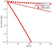
(b) SDCA; ijcnn1

Figure 1: mini-batch SAGA V.S. mini-batch SDCA

5.2 Importance sampling

We compare uniform sampling SAGA (SAGA-UNI) with importance sampling SAGA (SAGA-IP), as described in Section 3.3 , on three values of $\tau\in\{1,10,50\}$. The results for the datasets w8a and ijcnn1 are shown in Figure 2. For the dataset ijcnn1, mini-batch with importance sampling almost achieves linear speedup as the number of epochs does not increase with $\tau$. For the dataset w8a, mini-batch with importance sampling can even need less number of epochs than serial uniform sampling. Note that we adopt the importance sampling strategy described in Hanzely & Richtárik (2019) and the actual running time is the same as uniform sampling.

(a) ijcnn1

(b) w8a

Figure 2: importance sampling V.S. uniform sampling

5.3 Comparison with coordinate descent

We consider the un-regularized logistic regression problem (21) with $\lambda_{1}=\lambda_{2}=0$. In this case, Theorem 4.4 applies and we expect to have linear convergence of SAGA without any knowledge on the constant $\mu$ satsifying Assumption (4.2), see Remark 4.5. This makes SAGA comparable with descent methods such as gradient method and coordinate descent (CD) method. However, comparing with their deterministic counterparts, the speedup provided by CD can be at most of order $d$ while the speedup by SAGA can be of order $n$. Thus SAGA is much preferable than CD when $n$ is larger than $d$. We provide numerical evidence in Figure 3.

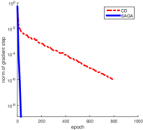
(a) ijcnn1

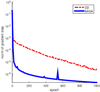
(b) a9a

Figure 3: SAGA V.S. CD

 

SUPPLEMENTARY MATERIAL
SAGA with Arbitrary Sampling

 

Appendix A Importance Sampling for Minibatches: Partition Sampling

In this section, we consider SAGA-AS with partition sampling for the problem

$$x^{*}=\arg\min_{x\in\mathbb{R}^{d}}\left[f(x)\;{:=}\;\sum_{i=1}^{n}\frac{1}{n}f_{i}(x)\right].$$ (23)

First we give the definition of partition of $[n]$ and partition sampling.

Definition A.1.

A partition ${\cal G}$ of $[n]$ is a set consisted of the subsets of $[n]$ such that $\cup_{C\in{\cal G}}C=[n]$ and $C_{i}\cap C_{j}=\emptyset$ for any $C_{i}$, $C_{j}\in{\cal G}$ with $i\neq j$. A partition sampling $S$ is a sampling such that $p_{C}=\mathbb{P}[S=C]>0$ for all $C\in{\cal G}$ and $\sum_{C\in{\cal G}}p_{C}=1$.

From (7) of Lemma 2.3, for partition sampling, we have ${\theta}_{C}^{i}=\frac{1}{p_{C}}$ if $i\in C$ for all $C\in{\cal G}$. Hence, SAGA-AS for problem (23) with partition sampling becomes Algorithm 2 (SAGA-PS):

Algorithm 2 SAGA with Partition Sampling for problem (23)–SAGA-PS

  Parameters: Partition sampling $S$ and stepsize $\alpha>0$

  Initialization: Choose $x^{0}\in\mathbb{R}^{d}$, ${\bf J}^{0}\in\mathbb{R}^{d\times n}$

  for  $k=0,1,2,...$ do

     Sample a fresh set $S_{k}\sim S$

     ${\bf J}^{k+1}={\bf J}^{k}+\left({\bf G}(x^{k})-{\bf J}^{k}\right){\bf\Pi}_{{\bf I}_{S_{k}}}$

     $g^{k}={\bf J}^{k}\lambda+\frac{1}{np_{S_{k}}}\left({\bf G}(x^{k})-{\bf J}^{k}\right){\bf\Pi}_{{\bf I}_{S_{k}}}e$

     $x^{k+1}=x^{k}-\alpha g^{k}$

  end for

Next we will give the iteration complexity of SAGA-PS by reformulation. For any partition sampling $S$, let $f_{C}(x)=\frac{1}{|C|}\sum_{i\in C}f_{i}(x)$ for $C\in{\cal G}$, and let $f_{C}$ be $L_{C}$-smooth. In problem (23), $\textstyle f(x)=\frac{1}{n}\sum_{i=1}^{n}f_{i}(x)=\frac{1}{n}\sum_{C\in{\cal G}}|C|f_{C}(x)=\sum_{C\in{\cal G}}\frac{|C|}{n}f_{C}(x).$ Let $m=|{\cal G}|$ and without loss of generality, we denote ${\cal G}=\{C_{1},C_{2},...,C_{m}\}$. Let $\lambda_{i}=\frac{|C_{i}|}{n}$ for $1\leq i\leq m$. Then we can see the minibatch SAGA with partition sampling for problem (23) (Algorithm 2) can be regarded as Algorithm 1 for problem (1) with the sampling: $\mathbb{P}[{\{i\}}]=p_{C_{i}}$ and ${\theta}_{\{i\}}^{j}=\frac{1}{p_{C_{i}}}$ for all $i$, $j\in[m]$. Hence, by applying Theorem 3.1, we can obtain the following theorem.

Theorem A.2.

Let $S$ be any partition sampling with partition ${\cal G}=\{C_{1},C_{2},...,C_{m}\}$. Let $f$ in problem (23) be $\mu$-strongly convex and $f_{C}$ be convex and $L_{C}$-smooth. Let $\{x^{k},{\bf J}^{k}\}$ be the iterates produced by Algorithm 2.
Consider the stochastic Lyapunov function

$$\Psi^{k}_{S}\;{:=}\;\|x^{k}-x^{*}\|^{2}+2\alpha\sigma_{S}\left\|\frac{1}{np_{S}}({\bf J}^{k}-{\bf G}(x^{k})){\Pi}_{{\bf I}_{S}}e\right\|^{2},$$

where $\sigma_{S}=\frac{n}{4L_{S}|S|}$ is a stochastic Lyapunov constant. If stepsize $\alpha$ satisfies

$$\alpha\leq\min_{C\in{\cal G}}\frac{p_{C}}{\mu+\frac{4L_{C}|C|}{n}},$$ (24)

then $\mathbb{E}[{\Psi}^{k}_{S}]\leq(1-\mu\alpha)^{k}\mathbb{E}[{\Psi}^{0}_{S}].$ This implies that if we choose $\alpha$ equal to the upper bound in (24), then

$$k\geq\max_{C\in{\cal G}}\left\{\frac{1}{p_{C}}+\frac{4L_{C}|C|}{\mu np_{C}}\right\}\log\left(\frac{1}{\epsilon}\right)\Rightarrow\mathbb{E}[{\Psi}^{k}_{S}]\leq\epsilon\cdot\mathbb{E}[{\Psi}^{0}_{S}].$$

Theorem A.2 contains Theorem 5.2 with $\tau$-partition sampling in Gower et al. (2018) as a special case, and with a little weaker condition: instead of demanding $f_{C}$ be $\mu$-strongly convex, we only need $f$ be $\mu$-strongly convex.

A.1 Partition sampling

From Theorem A.2, we can propose importance partition sampling for Algorithm 2. For a partition sampling $S$ with the partition ${\cal G}=\{C_{1},C_{2},...,C_{m}\}$, where $m=|{\cal G}|$, the iteration complexity of Algorithm 2 is given by

$$\max_{C\in{\cal G}}\left\{\frac{1}{p_{C}}+\frac{4L_{C}|C|}{\mu np_{C}}\right\}\log\left(\frac{1}{\epsilon}\right).$$

We can minimize the complexity bound in $p_{C}$ by choosing

$$p_{C}=\frac{\mu n+4L_{C}|C|}{\sum_{C\in{\cal G}}(\mu n+4L_{C}|C|)}.$$ (25)

With these optimal probabilities, the stepsize bound is $\alpha\leq\frac{n}{\sum_{C\in{\cal G}}(\mu n+4L_{C}|C|)}$, and by choosing the maximum allowed stepsize the resulting complexity becomes

$$\left(|{\cal G}|+\frac{4\sum_{C\in{\cal G}}L_{C}|C|}{\mu n}\right)\log\left(\frac{1}{\epsilon}\right).$$ (26)

Appendix B Proofs of Lemmas  2.3 and  3.2

B.1 Proof of Lemma 2.3

From (6), we know (5) in Assumption 2.1 is actually

$$\mathbb{E}[\theta_{S}{\rm Diag}(e_{S})\lambda]=\lambda,$$

which is equivalent to

$$\mathbb{E}[{\theta}^{i}_{S}1_{i\in S}\lambda_{i}]=\lambda_{i},$$

for all $i\in[n]$. Then for all $i\in[n]$, we have

$$\mathbb{E}[{\theta}^{i}_{S}1_{i\in S}\lambda_{i}] = \sum_{C\subseteq[n]}p_{C}{\theta}^{i}_{C}1_{i\in C}\lambda_{i}$$

$$= \sum_{C\subseteq[n]:i\in C}p_{C}{\theta}^{i}_{C}\lambda_{i}$$

$$= \lambda_{i}.$$

Since $\lambda_{i}>0$ for all $i\in[n]$, we have that (5) is equivalent to

$$\sum_{C\subseteq[n]:i\in C}p_{C}{\theta}^{i}_{C}=1,\quad\forall i\in[n].$$

B.2 Proof of Lemma 3.2(i)

From Lemma 2.3, the problem $\min_{\theta\in{\Theta}(S)}\beta_{i}$ is equivalent to the following linearly constrained convex problem:

$$\begin{array}[]{rcl}\min&&\beta_{i}=\sum_{C:i\in C}p_{C}|C|({\theta}_{C}^{i})^{2}\\ {\rm s.t.}&&\sum_{C:i\in C}p_{C}{\theta}_{C}^{i}=1.\end{array}$$ (27)

The KKT system of problem (27) is

$$\left\{\begin{array}[]{l}2p_{C}|C|{\theta}_{C}^{i}+{\tilde{\lambda}}p_{C}=0,\forall C:i\in C\\ \sum_{C:i\in C}p_{C}{\theta}_{C}^{i}=1,\end{array}\right.$$ (28)

where ${\tilde{\lambda}}\in\mathbb{R}$ is the Lagrangian dual variable. By solving system (28), we obtain the optimal solution

$${\theta}_{C}^{i}=\frac{1}{|C|\sum_{C:i\in C}\frac{p_{C}}{|C|}}=\frac{1}{p_{i}|C|\mathbb{E}^{i}[\frac{1}{|S|}]},$$

for all $C:i\in C$, and the minimum of $\beta_{i}$ is

$$\beta_{i} = \sum_{C:i\in C}p_{C}|C|({\theta}_{C}^{i})^{2}$$

$$= \sum_{C:i\in C}p_{C}|C|\frac{1}{(p_{i}|C|\mathbb{E}^{i}[\frac{1}{|S|}])^{2}}$$

$$= \frac{1}{p_{i}}\cdot\frac{1}{(\mathbb{E}^{i}[\frac{1}{|S|}])^{2}}\sum_{C:i\in C}\frac{p_{C}}{p_{i}}\frac{1}{|C|}$$

$$= \frac{1}{p_{i}}\cdot\frac{1}{\mathbb{E}^{i}[\frac{1}{|S|}]}.$$

B.3 Proof of Lemma 3.2(ii)

From (7) of Lemma 2.3, we can choose ${\theta}_{C}^{i}=\frac{1}{p_{i}}$ for all $i$ and $C$. Hence

$$\min_{\theta\in{\Theta}(S)}\beta_{i}\leq\sum_{C:i\in C}p_{C}|C|\frac{1}{p_{i}^{2}}=\frac{1}{p_{i}}\mathbb{E}^{i}[|S|],$$

which implies

$$\frac{1}{\mathbb{E}^{i}[\frac{1}{|S|}]}\leq\mathbb{E}^{i}[|S|].$$

Appendix C Smooth Case: Proof of Theorem 3.1

C.1 Lemmas

The following inequality is a direct consequence of convexity of $x\mapsto\|x\|^{2}$.

Lemma C.1.

Let $a^{i}\in\mathbb{R}^{d}$ for $1\leq i\leq z$ with $z\geq 1$. Then

$$\left\|\sum_{i=1}^{z}a^{i}\right\|^{2}\leq z\sum_{i=1}^{z}\|a^{i}\|^{2}.$$

Lemma C.2.

Let $S$ be a sampling, and $\sigma_{i}$ be any non-negative constant for $1\leq i\leq n$. Then

$$\mathbb{E}\left[|S|\sum_{i\in S}\sigma_{i}\left\|{\theta}_{S}^{i}\lambda_{i}({\bf J}^{k+1}_{:i}-\nabla f_{i}(x^{*}))\right\|^{2}\right] \leq \mathbb{E}\left[|S|\sum_{i\in S}(1-p_{i})\sigma_{i}\left\|{\theta}_{S}^{i}\lambda_{i}({\bf J}^{k}_{:i}-\nabla f_{i}(x^{*}))\right\|^{2}\right]$$

$$\quad+\mathbb{E}\left[\sum_{i=1}^{n}\sigma_{i}p_{i}\beta_{i}\lambda_{i}^{2}\left\|\nabla f_{i}(x^{k})-\nabla f_{i}(x^{*})\right\|^{2}\right].$$

Proof.

First notice that

$${\bf J}^{k+1}_{:i}=\left\{\begin{array}[]{rl}\nabla f_{i}(x^{k}),&\mbox{ if $i\in{S^{k}}$}\\ {\bf J}^{k}_{:i}.&\mbox{ if $i\notin S^{k}$ }\end{array}\right.$$

Then by taking conditional expectation on ${\bf J}^{k}$ and $x^{k}$, we have

$$\mathbb{E}\left[|S|\sum_{i\in S}\sigma_{i}\left\|{\theta}_{S}^{i}\lambda_{i}({\bf J}^{k+1}_{:i}-\nabla f_{i}(x^{*}))\right\|^{2}\;|\;{\bf J}^{k},x^{k}\right]$$

$$= \sum_{C}\sum_{\tilde{C}}\sum_{i\in C}p_{C}p_{\tilde{C}}|C|\sigma_{i}\left\|{\theta}_{C}^{i}\lambda_{i}({\bf J}^{k+1}_{:i}|_{S^{k}=\tilde{C}}-\nabla f_{i}(x^{*}))\right\|^{2}$$

$$= \sum_{C}p_{C}\sum_{i\in C}|C|\sigma_{i}({\theta}_{C}^{i})^{2}\lambda_{i}^{2}\sum_{\tilde{C}}p_{\tilde{C}}\left\|{\bf J}^{k+1}_{:i}|_{S^{k}=\tilde{C}}-\nabla f_{i}(x^{*})\right\|^{2}$$

$$= \sum_{C}p_{C}\sum_{i\in C}|C|\sigma_{i}({\theta}_{C}^{i})^{2}\lambda_{i}^{2}\left[\sum_{{\tilde{C}}:i\in{\tilde{C}}}p_{\tilde{C}}\left\|\nabla f_{i}(x^{k})-\nabla f(x^{*})\right\|^{2}+\sum_{{\tilde{C}}:i\notin{\tilde{C}}}p_{\tilde{C}}\left\|{\bf J}^{k}_{:i}-\nabla f_{i}(x^{*})\right\|^{2}\right]$$

$$= \sum_{C}p_{C}\sum_{i\in C}|C|\sigma_{i}({\theta}_{C}^{i})^{2}\lambda_{i}^{2}\left[p_{i}\left\|\nabla f_{i}(x^{k})-\nabla f(x^{*})\right\|^{2}+(1-p_{i})\left\|{\bf J}^{k}_{:i}-\nabla f_{i}(x^{*})\right\|^{2}\right]$$

$$= \mathbb{E}\left[|S|\sum_{i\in S}(1-p_{i})\sigma_{i}\left\|{\theta}_{S}^{i}\lambda_{i}({\bf J}^{k}_{:i}-\nabla f_{i}(x^{*}))\right\|^{2}\;|\;{\bf J}^{k},x^{k}\right]+\sum_{C}p_{C}\sum_{i\in C}|C|\sigma_{i}p_{i}({\theta}_{C}^{i})^{2}\lambda_{i}^{2}\left\|\nabla f_{i}(x^{k})-\nabla f_{i}(x^{*})\right\|^{2}$$

$$= \mathbb{E}\left[|S|\sum_{i\in S}(1-p_{i})\sigma_{i}\left\|{\theta}_{S}^{i}\lambda_{i}({\bf J}^{k}_{:i}-\nabla f_{i}(x^{*}))\right\|^{2}\;|\;{\bf J}^{k},x^{k}\right]+\sum_{i=1}^{n}\sigma_{i}p_{i}\lambda_{i}^{2}\sum_{C:i\in C}p_{C}|C|({\theta}_{C}^{i})^{2}\left\|\nabla f_{i}(x^{k})-\nabla f(x^{*})\right\|^{2}$$

$$= \mathbb{E}\left[|S|\sum_{i\in S}(1-p_{i})\sigma_{i}\left\|{\theta}_{S}^{i}\lambda_{i}({\bf J}^{k}_{:i}-\nabla f_{i}(x^{*}))\right\|^{2}\;|\;{\bf J}^{k},x^{k}\right]+\sum_{i=1}^{n}\sigma_{i}p_{i}\beta_{i}\lambda_{i}^{2}\left\|\nabla f_{i}(x^{k})-\nabla f_{i}(x^{*})\right\|^{2}.$$

Taking expectations again and applying the tower property, we obtain the result.

∎

In the next lemma we bound the second moment of the gradient estimate $g^{k}$.

Lemma C.3.

The second moment of the gradient estimate is bounded by

$$\mathbb{E}\left[\|g^{k}\|^{2}\;|\;{\bf J}^{k},x^{k}\right] \leq 2\mathbb{E}\left[|S|\sum_{i\in S}\left\|{\theta}_{S}^{i}\lambda_{i}({\bf J}^{k}_{:i}-\nabla f_{i}(x^{*}))\right\|^{2}\right]+2\sum_{i=1}^{n}\beta_{i}\lambda_{i}^{2}\left\|\nabla f_{i}(x^{k})-\nabla f_{i}(x^{*})\right\|^{2}.$$

Proof.

Recall that

$$g^{k} = {\bf J}^{k}\lambda+({\bf G}(x^{k})-{\bf J}^{k}){\theta}_{S_{k}}{\bf\Pi}_{{\bf I}_{S_{k}}}\lambda$$

$$= {\bf J}^{k}\lambda-({\bf J}^{k}-{\bf G}(x^{*})){\theta}_{S_{k}}{\bf\Pi}_{{\bf I}_{S_{k}}}\lambda+({\bf G}(x^{k})-{\bf G}(x^{*})){\theta}_{S_{k}}{\bf\Pi}_{{\bf I}_{S_{k}}}\lambda.$$

By applying Lemma C.1 with $z=2$, we get

$$\left\|g^{k}\right\|^{2}\leq 2\left\|({\bf G}(x^{k})-{\bf G}(x^{*})){\theta}_{S_{k}}{\bf\Pi}_{{\bf I}_{S_{k}}}\lambda\right\|^{2}+2\left\|({\bf J}^{k}-{\bf G}(x^{*})){\theta}_{S_{k}}{\bf\Pi}_{{\bf I}_{S_{k}}}\lambda-{\bf J}^{k}\lambda\right\|^{2},$$

which implies that

$$\mathbb{E}\left[\left\|g^{k}\right\|^{2}\;|\;{\bf J}^{k},x^{k}\right] \leq 2\mathbb{E}\left[\left\|({\bf G}(x^{k})-{\bf G}(x^{*})){\theta}_{S_{k}}{\bf\Pi}_{{\bf I}_{S_{k}}}\lambda\right\|^{2}\;|\;{\bf J}^{k},x^{k}\right]$$

$$\qquad+2\mathbb{E}\left[\left\|({\bf J}^{k}-{\bf G}(x^{*})){\theta}_{S_{k}}{\bf\Pi}_{{\bf I}_{S_{k}}}\lambda-{\bf J}^{k}\lambda\right\|^{2}\;|\;{\bf J}^{k},x^{k}\right].$$

For $\mathbb{E}\left[\left\|({\bf G}(x^{k})-{\bf G}(x^{*})){\theta}_{S_{k}}{\bf\Pi}_{{\bf I}_{S_{k}}}\lambda\right\|^{2}\;|\;{\bf J}^{k},x^{k}\right]$, by applying Lemma C.1 with $z=|C|$, we get

$$\mathbb{E}\left[\left\|({\bf G}(x^{k})-{\bf G}(x^{*})){\theta}_{S_{k}}{\bf\Pi}_{{\bf I}_{S_{k}}}\lambda\right\|^{2}\;|\;{\bf J}^{k},x^{k}\right] = \sum_{C}p_{C}\left\|({\bf G}(x^{k})-{\bf G}(x^{*})){\theta}_{C}{\bf\Pi}_{{\bf I}_{C}}\lambda\right\|^{2}$$

$$\leq \sum_{C}p_{C}|C|\sum_{i\in C}\left\|{\theta}_{C}^{i}\lambda_{i}(\nabla f_{i}(x^{k})-\nabla f_{i}(x^{*}))\right\|^{2}$$

$$= \sum_{i=1}^{n}\lambda_{i}^{2}\sum_{C:i\in C}p_{C}|C|({\theta}_{C}^{i})^{2}\left\|\nabla f_{i}(x^{k})-\nabla f_{i}(x^{*})\right\|^{2}$$

$$= \sum_{i=1}^{n}\beta_{i}\lambda_{i}^{2}\left\|\nabla f_{i}(x^{k})-\nabla f_{i}(x^{*})\right\|^{2}.$$

For $\mathbb{E}\left[\left\|({\bf J}^{k}-{\bf G}(x^{*})){\theta}_{S_{k}}{\bf\Pi}_{{\bf I}_{S_{k}}}\lambda-{\bf J}^{k}\lambda\right\|^{2}\;|\;{\bf J}^{k},x^{k}\right]$, since

$$\mathbb{E}\left[({\bf J}^{k}-{\bf G}(x^{*})){\theta}_{S_{k}}{\bf\Pi}_{{\bf I}_{S_{k}}}\lambda\;|\;{\bf J}^{k},x^{k}\right]={\bf J}^{k}\lambda,$$

and $\mathbb{E}[\|X-\mathbb{E}[X]\|^{2}]\leq\mathbb{E}[\|X\|^{2}]$, we have that

$$\mathbb{E}\left[\left\|({\bf J}^{k}-{\bf G}(x^{*})){\theta}_{S_{k}}{\bf\Pi}_{{\bf I}_{S_{k}}}\lambda-{\bf J}^{k}\lambda\right\|^{2}\;|\;{\bf J}^{k},x^{k}\right] \leq \mathbb{E}\left[\left\|({\bf J}^{k}-{\bf G}(x^{*})){\theta}_{S_{k}}{\bf\Pi}_{{\bf I}_{S_{k}}}\lambda\right\|^{2}\;|\;{\bf J}^{k},x^{k}\right]$$

$$= \sum_{C}p_{C}\left\|{\bf J}^{k}-{\bf G}(x^{*})){\theta}_{C}{\bf\Pi}_{{\bf I}_{C}}\lambda\right\|^{2}$$

$$\leq \sum_{C}p_{C}|C|\sum_{i\in C}\left\|{\theta}_{C}^{i}\lambda_{i}({\bf J}^{k}_{:i}-\nabla f_{i}(x^{*}))\right\|^{2}$$

$$= \mathbb{E}\left[|S|\sum_{i\in S}\left\|{\theta}_{S}^{i}\lambda_{i}({\bf J}^{k}_{:i}-\nabla f_{i}(x^{*}))\right\|^{2}\;|\;{\bf J}^{k},x^{k}\right],$$

where the second inequality comes from Lemma C.1 with $z=|C|$.

Finally, we arrive at the result

$$\mathbb{E}\left[\|g^{k}\|^{2}\;|\;{\bf J}^{k},x^{k}\right]\leq 2\mathbb{E}\left[|S|\sum_{i\in S}\left\|{\theta}_{S}^{i}\lambda_{i}({\bf J}^{k}_{:i}-\nabla f_{i}(x^{*}))\right\|^{2}\;|\;{\bf J}^{k},x^{k}\right]+2\sum_{i=1}^{n}\beta_{i}\lambda_{i}^{2}\left\|\nabla f_{i}(x^{k})-\nabla f_{i}(x^{*})\right\|^{2}.$$

∎

Lemma C.4.

If $f$ is $\mu$-strongly convex, and $f_{i}$ is convex and $L_{i}$-smooth, then

$$\langle\nabla f(x)-\nabla f(y),x-y\rangle\geq\frac{\mu}{2}\|x-y\|^{2}+\sum_{i=1}^{n}\frac{\lambda_{i}}{2L_{i}}\left\|\nabla f_{i}(x)-\nabla f_{i}(y)\right\|^{2},$$

for all $x$, $y\in\mathbb{R}^{d}$.

Proof.

Since $f$ is $\mu$-strongly convex, we have

$$\langle\nabla f(x)-\nabla f(y),x-y\rangle\geq\mu\|x-y\|^{2}.$$ (29)

Since $f_{i}$ is $L_{i}$-smooth, we have

$$\langle\nabla f_{i}(x)-\nabla f_{i}(y),x-y\rangle\geq\frac{1}{L_{i}}\|\nabla f_{i}(x)-\nabla f_{i}(y)\|^{2},$$

which indicates

$$\langle\nabla f(x)-\nabla f(y),x-y\rangle\geq\sum_{i=1}^{n}\frac{\lambda_{i}}{L_{i}}\|\nabla f_{i}(x)-\nabla f_{i}(y)\|^{2}.$$ (30)

Combining (29) and (30), we can get

$$\langle\nabla f(x)-\nabla f(y),x-y\rangle\geq\frac{\mu}{2}\|x-y\|^{2}+\sum_{i=1}^{n}\frac{\lambda_{i}}{2L_{i}}\|\nabla f_{i}(x)-\nabla f_{i}(y)\|^{2}.$$

∎

C.2 Proof of Theorem 3.1

Having established the above lemmas, we are ready to proceed to the proof of pour main theorem covering the smooth case (Theorem 3.1).

Let $\mathbb{E}_{k}[\cdot]$ denote the expectation conditional on ${\bf J}^{k}$ and $x^{k}$. First, from Assumption 2.1, it is evident that

$$\mathbb{E}_{k}[g^{k}]={\bf J}^{k}\lambda+\nabla f(x^{k})-{\bf J}^{k}\lambda=\nabla f(x^{k}).$$ (31)

Then we can obtain

$$\mathbb{E}_{k}\left[\|x^{k+1}-x^{*}\|^{2}\right] = \mathbb{E}_{k}\left[\|x^{k}-x^{*}-\alpha g^{k}\|^{2}\right]$$

$$\overset{(\ref{expgk})}{=} \|x^{k}-x^{*}\|^{2}-2\alpha\langle\nabla f(x^{k}),x^{k}-x^{*}\rangle+\alpha^{2}\mathbb{E}_{k}[\|g^{k}\|^{2}]$$

$$\overset{\rm Lemma~{}\ref{lm:nablafx}}{\leq} (1-\mu\alpha)\|x^{k}-x^{*}\|^{2}-2\alpha\sum_{i=1}^{n}\frac{\lambda_{i}}{2L_{i}}\|\nabla f_{i}(x^{k})-\nabla f_{i}(x^{*})\|^{2}+\alpha^{2}\mathbb{E}_{k}[\|g^{k}\|^{2}]$$

$$\overset{\rm Lemma~{}\ref{lm:gk2}}{\leq} (1-\mu\alpha)\|x^{k}-x^{*}\|^{2}+2\alpha\sum_{i=1}^{n}\left[(\alpha\beta_{i}\lambda_{i}^{2}-\frac{\lambda_{i}}{2L_{i}})\|\nabla f_{i}(x^{k})-\nabla f_{i}(x^{*})\|^{2}\right]$$

$$+2\alpha^{2}\mathbb{E}_{k}\left[|S|\sum_{i\in S}\left\|{\theta}_{S}^{i}\lambda_{i}({\bf J}^{k}_{:i}-\nabla f_{i}(x^{*}))\right\|^{2}\right]$$

Taking expectation again and applying the tower property, we obtain

$$\mathbb{E}\left[\|x^{k+1}-x^{*}\|^{2}\right] \leq (1-\mu\alpha)\mathbb{E}\left[\|x^{k}-x^{*}\|^{2}\right]+2\alpha\mathbb{E}\left[\sum_{i=1}^{n}\left((\alpha\beta_{i}\lambda_{i}^{2}-\frac{\lambda_{i}}{2L_{i}})\left\|\nabla f_{i}(x^{k})-\nabla f_{i}(x^{*})\right\|^{2}\right)\right]$$

$$+2\alpha^{2}\mathbb{E}\left[|S|\sum_{i\in S}\left\|{\theta}_{S}^{i}\lambda_{i}({\bf J}^{k}_{:i}-\nabla f_{i}(x^{*}))\right\|^{2}\right].$$

Therefore, for the stochastic Lyapunov function $\Psi^{k+1}_{S}$, we have

$$\mathbb{E}[\Psi^{k+1}_{S}] \leq (1-\mu\alpha)\mathbb{E}\left[\|x^{k}-x^{*}\|^{2}\right]+2\alpha\mathbb{E}\left[\sum_{i=1}^{n}\left(\left(\alpha\beta_{i}\lambda_{i}^{2}-\frac{\lambda_{i}}{2L_{i}}\right)\left\|\nabla f_{i}(x^{k})-\nabla f_{i}(x^{*})\right\|^{2}\right)\right]$$

$$+2\alpha^{2}\mathbb{E}\left[|S|\sum_{i\in S}\left\|{\theta}_{S}^{i}\lambda_{i}({\bf J}^{k}_{:i}-\nabla f_{i}(x^{*}))\right\|^{2}\right]+2\alpha\mathbb{E}\left[|S|\sum_{i\in S}\sigma_{i}\left\|{\theta}_{S}^{i}\lambda_{i}({\bf J}^{k+1}_{:i}-\nabla f_{i}(x^{*}))\right\|^{2}\right]$$

$$\overset{\rm Lemma\ref{lm:Jk+1}}{\leq} \mathbb{E}\left[(1-\mu\alpha)\|x^{k}-x^{*}\|^{2}\right]+2\alpha\mathbb{E}\left[\sum_{i=1}^{n}\left((\alpha\beta_{i}\lambda_{i}^{2}-\frac{\lambda_{i}}{2L_{i}}+\sigma_{i}p_{i}\beta_{i}\lambda_{i}^{2})\left\|\nabla f_{i}(x^{k})-\nabla f_{i}(x^{*})\right\|^{2}\right)\right]$$

$$+2\alpha\mathbb{E}\left[|S|\sum_{i\in S}[(1-p_{i})\sigma_{i}+\alpha]\left\|{\theta}_{S}^{i}\lambda_{i}({\bf J}^{k}_{:i}-\nabla f_{i}(x^{*}))\right\|^{2}\right]$$

In order to guarantee that $\mathbb{E}{\Psi^{k+1}_{S}}\leq(1-\mu\alpha)\mathbb{E}{\Psi^{k}_{S}}$, $\alpha$ should be chosen such that

$$\alpha\beta_{i}\lambda_{i}^{2}-\frac{\lambda_{i}}{2L_{i}}+\sigma_{i}p_{i}\beta_{i}\lambda_{i}^{2}\leq 0,\quad\Rightarrow\quad\alpha\leq\frac{1}{2L_{i}\beta_{i}\lambda_{i}}-\sigma_{i}p_{i},$$

and

$$(1-p_{i})\sigma_{i}+\alpha\leq(1-\mu\alpha)\sigma_{i},\quad\Rightarrow\quad\alpha\leq\frac{\sigma_{i}p_{i}}{\mu\sigma_{i}+1},$$

for all $1\leq i\leq n$. Since $\sigma_{i}=\frac{1}{4L_{i}\beta_{i}p_{i}\lambda_{i}}$, if $\alpha$ satisfies

$$\alpha\leq\min_{1\leq i\leq n}\frac{p_{i}}{\mu+4L_{i}\beta_{i}\lambda_{i}p_{i}},$$

then we have the recursion $\mathbb{E}{\Psi^{k+1}_{S}}\leq(1-\mu\alpha)\mathbb{E}{\Psi^{k}_{S}}$.

C.3 Proof of Theorem A.2

In problem (23),

$$f(x)=\sum_{C\in{\cal G}}\frac{|C|}{n}f_{C}(x)=\sum_{i=1}^{m}\frac{|C_{i}|}{n}f_{C_{i}}(x).$$

Hence by choosing ${\tilde{f}}_{i}=f_{C_{i}}$ and ${\tilde{\lambda}}_{i}=\frac{|C_{i}|}{n}$ for $1\leq i\leq m$, problem (23) has the same form as problem (1), and the Lipschitz smothness constant ${\tilde{L}}_{i}$ of ${\tilde{f}}_{i}$ is $L_{C_{i}}$.

From the partition sampling $S$, we can construct a sampling $\tilde{S}$ from $S$ as follows: ${\tilde{S}}(S)=\{i\}$ if $S=C_{i}$. It is obvious that $\mathbb{P}[{\tilde{S}}=\{i\}]=p_{C_{i}}$ for all $1\leq i\leq m$. For sampling $\tilde{S}$, we choose ${\theta}_{\tilde{S}}$ be such that ${\theta}_{\{i\}}=\frac{1}{p_{C_{i}}}{\bf I}$. For the sampling $\tilde{S}$ and ${\theta}_{\tilde{S}}$, the corresponding ${\tilde{\beta}}_{i}=\frac{1}{p_{C_{i}}}$ from (8).

Let ${\tilde{S}}_{k}(S_{k})=\{i\}$ if $S_{k}=C_{i}$ for $k\geq 0$. Then ${\tilde{S}}_{k}\sim{\tilde{S}}$ is equivalent to $S_{k}\sim S$. Let $\{{\tilde{x}}^{k},{\tilde{\bf J}}^{k}\}$ be produced by Algorithm 1 with ${\tilde{\lambda}}_{i}$, ${\tilde{f}}_{i}$, $\tilde{S}$, and ${\theta}_{\tilde{S}}$. Then it is easy to see that

$$\left\{\begin{array}[]{l}{\tilde{x}}^{k}=x^{k},\\ {\tilde{\bf J}}^{k}_{:i}=\frac{1}{|C_{i}|}{\bf J}^{k}{\Pi}_{{\bf I}_{C_{i}}}e,\ \forall 1\leq i\leq m.\end{array}\right.$$ (32)

Therefore, by applying Theorem 3.1 to $\{{\tilde{x}}^{k},{\tilde{\bf J}}^{k}\}$, we can get the results.

Appendix D Nonsmooth Case: Proofs of Theorems 4.4 and 4.6

D.1 Lemmas

Lemma D.1.

Let $\mathbb{E}_{k}[\cdot]$ denote the expectation conditional on ${\bf J}^{k}$ and $x^{k}$. First, from Assumption 2.1, it is evident that

$$\mathbb{E}_{k}[g^{k}]={\bf J}^{k}\lambda+\nabla f(x^{k})-{\bf J}^{k}\lambda=\nabla f(x^{k}).$$ (33)

Lemma D.2.

Under Assumption 4.1 and Assumption 4.3, for any $x^{*},y^{*}\in\mathcal{X}^{*}$ and $x\in\mathbb{R}^{d}$, we have,

$$\langle\nabla f(x)-\nabla f(y^{*}),x-y^{*}\rangle\geq\gamma\sum_{i=1}^{n}\lambda_{i}\left\|\nabla\phi_{i}({\bf A}_{i}^{\top}x)-\nabla\phi_{i}({\bf A}_{i}^{\top}x^{*})\right\|^{2}.$$

Proof.

Since $\phi_{i}$ is $1/\gamma$-smooth, we have

$$\langle\nabla\phi_{i}(\tilde{x})-\nabla\phi_{i}(\tilde{y}),{\tilde{x}}-{\tilde{y}}\rangle\geq\gamma\left\|\nabla\phi_{i}(\tilde{x})-\nabla\phi_{i}(\tilde{y})\right\|^{2},\enspace\forall i=1,\cdots,n.$$

Let $\tilde{x}={\bf A}_{i}^{\top}x$, and $\tilde{y}={\bf A}_{i}^{\top}y^{*}$ in the above inequlity. Then we get

$$\langle\nabla\phi_{i}({\bf A}_{i}^{\top}x)-\nabla\phi_{i}({\bf A}_{i}^{\top}y^{*}),{\bf A}_{i}(x-y^{*})\rangle\geq\gamma\left\|\nabla\phi_{i}({\bf A}_{i}^{\top}x)-\nabla\phi_{i}({\bf A}_{i}^{\top}y^{*})\right\|^{2},\enspace\forall i=1,\cdots,n,$$

which is actually

$$\langle\nabla f_{i}(x)-\nabla f_{i}(y^{*}),x-y^{*}\rangle\geq\gamma\left\|\nabla\phi_{i}({\bf A}_{i}^{\top}x)-\nabla\phi_{i}({\bf A}_{i}^{\top}y^{*})\right\|^{2},\enspace\forall i=1,\cdots,n,$$

Summing over $i$ we get

$$\langle\nabla f(x)-\nabla f(y^{*}),x-y^{*}\rangle\geq\gamma\sum_{i=1}^{n}\lambda_{i}\left\|\nabla\phi_{i}({\bf A}_{i}^{\top}x)-\nabla\phi_{i}({\bf A}_{i}^{\top}y^{*})\right\|^{2}$$

The statement then follows directly from Assumption 4.3. ∎

We now quote a result from Poon et al. (2018).

Theorem D.3.

[Poon et al. (2018)] If if $f$ is $L$-smooth and $\alpha\leq\frac{1}{3L}$, then almost surely the sequence $P(x^{k})$ is bounded.

Lemma D.4.

Under Assumption 4.2, if $f$ is $L$-smooth and $\alpha\leq\frac{1}{3L}$, then there is $\mu>0$ such that for all $k\geq 0$,

$$\mathbb{E}_{k}\left[\|x^{k+1}-[x^{k+1}]^{*}\|^{2}\right]\leq\frac{1}{1+\mu\alpha}\mathbb{E}_{k}\left[\|x^{k}-[x^{k}]^{*}\|^{2}\right]+\frac{2\alpha^{2}}{1+\mu\alpha}\mathbb{E}_{k}\left[\|g^{k}-\nabla f(x^{k})\|^{2}\right]$$

Proof.

Since

$$x^{k+1}=\arg\min\left\{\frac{1}{2\alpha}\|y-x^{k}+\alpha g^{k}\|^{2}+\psi(y)\right\},$$

we know $\alpha^{-1}(x^{k}-x^{k+1})-g^{k}\in\partial\psi(x^{k+1})$. Using the convexity of $f$ and $\psi$, we obtain

$$P^{*}\geq f(x^{k})+\langle\nabla f(x^{k}),[x^{k}]^{*}-x^{k}\rangle+\psi(x^{k+1})+\langle\alpha^{-1}(x^{k}-x^{k+1})-g^{k},[x^{k}]^{*}-x^{k+1}\rangle.$$ (34)

Next we bound $f(x^{k+1})$ by $f(x^{k})$. Since $f$ is $L$-smooth, we have

$$f(x^{k+1})\leq f(x^{k})+\langle\nabla f(x^{k}),x^{k+1}-x^{k}\rangle+\frac{L}{2}\|x^{k+1}-x^{k}\|^{2}.$$ (35)

Combining (34) and (35) we get

$$f(x^{k+1})+\psi(x^{k+1})-P^{*} \leq \langle\nabla f(x^{k}),x^{k+1}-[x^{k}]^{*}\rangle+\frac{L}{2}\|x^{k+1}-x^{k}\|^{2}$$

$$\qquad\quad-\langle\alpha^{-1}(x^{k}-x^{k+1})-g^{k},[x^{k}]^{*}-x^{k+1}\rangle$$

$$= \frac{L}{2}\|x^{k+1}-x^{k}\|^{2}-\frac{1}{\alpha}\langle x^{k}-x^{k+1},[x^{k}]^{*}-x^{k+1}\rangle+\langle\nabla f(x^{k})-g^{k},[x^{k}]^{*}-x^{k+1}\rangle$$

$$= \left(\frac{L}{2}-\frac{1}{2\alpha}\right)\|x^{k+1}-x^{k}\|^{2}-\frac{1}{2\alpha}\|x^{k+1}-x^{k}\|^{2}$$

$$\qquad-\frac{1}{\alpha}\langle x^{k}-x^{k+1},[x^{k}]^{*}-x^{k}\rangle+\langle\nabla f(x^{k})-g^{k},[x^{k}]^{*}-x^{k+1}\rangle$$

$$\leq -\frac{1}{2\alpha}\|x^{k+1}-x^{k}\|^{2}-\frac{1}{\alpha}\langle x^{k}-x^{k+1},[x^{k}]^{*}-x^{k}\rangle+\langle\nabla f(x^{k})-g^{k},[x^{k}]^{*}-x^{k+1}\rangle$$

$$= -\frac{1}{2\alpha}\|x^{k+1}-[x^{k}]^{*}\|^{2}+\frac{1}{2\alpha}\|x^{k}-[x^{k}]^{*}\|^{2}+\langle\nabla f(x^{k})-g^{k},[x^{k}]^{*}-x^{k+1}\rangle.$$

Now we use Assumption 4.2 and Theorem D.3 to obtain the existence of $\mu>0$ such that

$${(\mu\alpha+1)}\|x^{k+1}-[x^{k+1}]^{*}\|^{2}\leq\|x^{k}-[x^{k}]^{*}\|^{2}+2\alpha\langle\nabla f(x^{k})-g^{k},[x^{k}]^{*}-x^{k+1}\rangle.$$

Taking conditional expectation on both side, we get

$$\mathbb{E}_{k}\left[\|x^{k+1}-[x^{k+1}]^{*}\|^{2}\right]\leq\frac{1}{\mu\alpha+1}\mathbb{E}_{k}\left[\|x^{k}-[x^{k}]^{*}\|^{2}\right]+\frac{2\alpha}{\mu\alpha+1}\mathbb{E}_{k}\left[\langle\nabla f(x^{k})-g^{k},[x^{k}]^{*}-x^{k+1}\rangle\right]$$

$$\overset{\eqref{expgk2}}{=}\frac{1}{\mu\alpha+1}\mathbb{E}_{k}\left[\|x^{k}-[x^{k}]^{*}\|^{2}\right]+\frac{2\alpha}{\mu\alpha+1}\mathbb{E}_{k}\left[\langle\nabla f(x^{k})-g^{k},\bar{x}^{k+1}-x^{k+1}\rangle\right],$$

where $\bar{x}^{k+1}=\operatorname{prox}^{\psi}_{\alpha}(x^{k}-\alpha\nabla f(x^{k}))$ is determined by $x^{k}$. Recall that ${x}^{k+1}=\operatorname{prox}^{\psi}_{\alpha}(x^{k}-\alpha g^{k})$. We use the non-expansiveness of the proximal mapping:

$$\|\bar{x}^{k+1}-x^{k+1}\|\leq\alpha\|\nabla f(x^{k})-g^{k}\|.$$

Then the statement follows by the Cauchy-Schwarz inequality. ∎

Lemma D.5.

$$\mathbb{E}\left[\sum_{i=1}^{n}\sigma_{i}p_{i}^{-1}v_{i}\lambda_{i}^{2}\left\|\alpha_{i}^{k+1}-\nabla\phi_{i}({\bf A}_{i}^{\top}x^{*})\right\|^{2}\right] \leq \mathbb{E}\left[\sum_{i=1}^{n}\sigma_{i}v_{i}\lambda_{i}^{2}\left\|\nabla\phi({\bf A}_{i}^{\top}x^{k})-\nabla\phi_{i}({\bf A}_{i}^{\top}x^{*})\right\|^{2}\right]$$

$$\qquad+\mathbb{E}\left[\sum_{i=1}^{n}\sigma_{i}p_{i}^{-1}v_{i}\lambda_{i}^{2}(1-p_{i})\left\|\alpha_{i}^{k}-\nabla\phi_{i}({\bf A}_{i}^{\top}x^{*})\right\|^{2}\right]$$

Proof.

First notice that

$$\alpha^{k+1}_{i}=\left\{\begin{array}[]{ll}\nabla\phi({\bf A}_{i}^{\top}x^{k}),&\mbox{ if $i\in{S^{k}}$}\\ \alpha_{i}^{k},&\mbox{ if $i\notin S^{k}$ }\end{array}\right.$$

Then by taking conditional expectation on $\alpha^{k}$, we have

$$\mathbb{E}\left[\sum_{i=1}^{n}\sigma_{i}p_{i}^{-1}v_{i}\lambda_{i}^{2}\left\|\alpha_{i}^{k+1}-\nabla\phi_{i}({\bf A}_{i}^{\top}x^{*})\right\|^{2}\;|\;\alpha^{k}\right]$$

$$= \sum_{i=1}^{n}\sigma_{i}p_{i}^{-1}v_{i}\lambda_{i}^{2}\mathbb{E}\left[\left\|\alpha_{i}^{k+1}-\nabla\phi_{i}({\bf A}_{i}^{\top}x^{*})\right\|^{2}|\alpha^{k}\right]$$

$$= \sum_{i=1}^{n}\sigma_{i}p_{i}^{-1}v_{i}\lambda_{i}^{2}\left(p_{i}\|\nabla\phi_{i}({\bf A}_{i}^{\top}x^{k})-\nabla\phi_{i}({\bf A}_{i}^{\top}x^{*})\|^{2}+(1-p_{i})\left\|\alpha_{i}^{k}-\nabla\phi_{i}({\bf A}_{i}^{\top}x^{*})\right\|^{2}\right).$$

Taking expectations again and applying the tower property, we obtain the result.

∎

Lemma D.6.

For any $x^{*},y^{*}\in\mathcal{X}^{*}$,

$$\mathbb{E}\left[\|g^{k}-\nabla f(y^{*})\|^{2}\;|\;{\bf J}^{k},x^{k}\right]\leq 2\sum_{i=1}^{n}p_{i}^{-1}v_{i}\lambda_{i}^{2}\left\|\nabla\phi_{i}({\bf A}_{i}^{\top}x^{k})-\nabla\phi_{i}({\bf A}_{i}^{\top}x^{*})\right\|^{2}+2\sum_{i=1}^{n}p_{i}^{-1}v_{i}\lambda_{i}^{2}\left\|\alpha_{i}^{k}-\nabla\phi_{i}({\bf A}_{i}^{\top}x^{*})\right\|^{2}.$$

Proof.

Recall that

$$g^{k} = {\bf J}^{k}\lambda+\left({\bf G}(x^{k})-{\bf J}^{k}\right){\theta}_{S_{k}}{\bf\Pi}_{{\bf I}_{S_{k}}}\lambda$$

$$= {\bf J}^{k}\lambda-\left({\bf J}^{k}-{\bf G}(x^{*})\right){\theta}_{S_{k}}{\bf\Pi}_{{\bf I}_{S_{k}}}\lambda+({\bf G}(x^{k})-{\bf G}(x^{*})){\theta}_{S_{k}}{\bf\Pi}_{{\bf I}_{S_{k}}}\lambda.$$

By applying Lemma C.1 with $z=2$, we get

$$\|g^{k}-\nabla f(y^{*})\|^{2}\leq 2\left\|({\bf G}(x^{k})-{\bf G}(x^{*})){\theta}_{S_{k}}{\bf\Pi}_{{\bf I}_{S_{k}}}\lambda\right\|^{2}+2\left\|({\bf J}^{k}-{\bf G}(x^{*})){\theta}_{S_{k}}{\bf\Pi}_{{\bf I}_{S_{k}}}\lambda-{\bf J}^{k}\lambda+\nabla f(y^{*})\right\|^{2},$$

which implies that

$$\mathbb{E}\left[\|g^{k}-\nabla f(y^{*})\|^{2}\;|\;{\bf J}^{k},x^{k}\right] \leq 2\mathbb{E}\left[\left\|({\bf G}(x^{k})-{\bf G}(x^{*})){\theta}_{S_{k}}{\bf\Pi}_{{\bf I}_{S_{k}}}\lambda\right\|^{2}\;|\;{\bf J}^{k},x^{k}\right]$$

$$\qquad+2\mathbb{E}\left[\left\|({\bf J}^{k}-{\bf G}(x^{*})){\theta}_{S_{k}}{\bf\Pi}_{{\bf I}_{S_{k}}}\lambda-{\bf J}^{k}\lambda+\nabla f(y^{*})\right\|^{2}\;|\;{\bf J}^{k},x^{k}\right]$$

$$\leq 2\mathbb{E}\left[\left\|({\bf G}(x^{k})-{\bf G}(x^{*})){\theta}_{S_{k}}{\bf\Pi}_{{\bf I}_{S_{k}}}\lambda\right\|^{2}\;|\;{\bf J}^{k},x^{k}\right]$$

$$\qquad+2\mathbb{E}\left[\left\|({\bf J}^{k}-{\bf G}(x^{*})){\theta}_{S_{k}}{\bf\Pi}_{{\bf I}_{S_{k}}}\lambda\right\|^{2}\;|\;{\bf J}^{k},x^{k}\right],$$

where the last inequality follows from

$$\mathbb{E}\left[({\bf J}^{k}-{\bf G}(x^{*})){\theta}_{S_{k}}{\bf\Pi}_{{\bf I}_{S_{k}}}\lambda\;|\;{\bf J}^{k},x^{k}\right]={\bf J}^{k}\lambda-\nabla f(x^{*})\overset{Assumption~{}\ref{ass:uniquegradient}}{=}{\bf J}^{k}\lambda-\nabla f(y^{*})$$

and $\mathbb{E}[\|X-\mathbb{E}[X]\|^{2}]\leq\mathbb{E}[\|X\|^{2}]$. Hence,

$$\mathbb{E}\left[\|g^{k}-\nabla f(x^{*})\|^{2}\;|\;{\bf J}^{k},x^{k}\right] \leq 2\mathbb{E}\left[\left\|\sum_{i\in S_{k}}p_{i}^{-1}\lambda_{i}{\bf A}_{i}\left(\phi_{i}^{\prime}({\bf A}_{i}^{\top}x^{k})-\phi^{\prime}_{i}({\bf A}_{i}^{\top}x^{*})\right)\right\|^{2}\;|\;{\bf J}^{k},x^{k}\right]$$

$$\qquad+2\mathbb{E}\left[\left\|\sum_{i\in S_{k}}p_{i}^{-1}\lambda_{i}{\bf A}_{i}\left(\alpha^{k}-\phi^{\prime}_{i}({\bf A}_{i}^{\top}x^{*})\right)\right\|^{2}\;|\;{\bf J}^{k},x^{k}\right]$$

$$\overset{\eqref{eq:ESOfirst}}{\leq} 2\sum_{i=1}^{n}p_{i}^{-1}v_{i}\lambda_{i}^{2}\left\|\phi_{i}^{\prime}({\bf A}_{i}^{\top}x^{k})-\phi^{\prime}_{i}({\bf A}_{i}^{\top}x^{*})\right\|^{2}+2\sum_{i=1}^{n}p_{i}^{-1}v_{i}\lambda_{i}^{2}\left\|\alpha_{i}^{k}-\phi^{\prime}_{i}({\bf A}_{i}^{\top}x^{*})\right\|^{2}.$$

∎

Lemma D.7.

For any $x^{*}\in\mathcal{X}^{*}$,

$$\mathbb{E}\left[\|g^{k}-\nabla f(x^{k})\|^{2}\;|\;{\bf J}^{k},x^{k}\right]\leq 2\sum_{i=1}^{n}p_{i}^{-1}v_{i}\lambda_{i}^{2}\left\|\nabla\phi_{i}({\bf A}_{i}^{\top}x^{k})-\nabla\phi_{i}({\bf A}_{i}^{\top}x^{*})\right\|^{2}+2\sum_{i=1}^{n}p_{i}^{-1}v_{i}\lambda_{i}^{2}\left\|\alpha_{i}^{k}-\nabla\phi_{i}({\bf A}_{i}^{\top}x^{*})\right\|^{2}.$$

Proof.

$$g^{k}-\nabla f(x^{k}) = {\bf J}^{k}\lambda-({\bf J}^{k}-{\bf G}(x^{*})){\theta}_{S_{k}}{\bf\Pi}_{{\bf I}_{S_{k}}}\lambda+({\bf G}(x^{k})-{\bf G}(x^{*})){\theta}_{S_{k}}{\bf\Pi}_{{\bf I}_{S_{k}}}\lambda-\nabla f(x^{k})$$

$$= {\bf J}^{k}\lambda-({\bf J}^{k}-{\bf G}(x^{*})){\theta}_{S_{k}}{\bf\Pi}_{{\bf I}_{S_{k}}}\lambda-\nabla f(x^{*})$$

$$\qquad\quad+({\bf G}(x^{k})-{\bf G}(x^{*})){\theta}_{S_{k}}{\bf\Pi}_{{\bf I}_{S_{k}}}\lambda-\nabla f(x^{k})+\nabla f(x^{*}).$$

The rest of the proof is the same as in Lemma D.6. ∎

D.2 Proof of Theorem 4.4

For any $x^{*}\in\mathcal{X}^{*}$, we have

$$x^{*}=\operatorname{prox}^{\psi}_{\alpha}(x^{*}-\alpha\nabla f(x^{*})).$$

Therefore,

$$\mathbb{E}_{k}\left[\left\|x^{k+1}-[x^{k+1}]^{*}\right\|^{2}\right]$$

$$\leq \mathbb{E}_{k}\left[\left\|x^{k+1}-[x^{k}]^{*}\right\|^{2}\right]$$

$$= \mathbb{E}_{k}\left[\left\|\operatorname{prox}^{\psi}_{\alpha}(x^{k}-\alpha g^{k})-[x^{k}]^{*}\right\|^{2}\right]$$

$$= \mathbb{E}_{k}\left[\left\|\operatorname{prox}^{\psi}_{\alpha}(x^{k}-\alpha g^{k})-\operatorname{prox}^{\psi}_{\alpha}([x^{k}]^{*}-\alpha\nabla f([x^{k}]^{*}))\right\|^{2}\right]$$

$$\leq \mathbb{E}_{k}\left[\left\|x^{k}-\alpha g^{k}-([x^{k}]^{*}-\alpha\nabla f([x^{k}]^{*}))\right\|^{2}\right]$$

$$\overset{(\ref{expgk2})}{=} \left\|x^{k}-[x^{k}]^{*}\right\|^{2}-2\alpha\langle\nabla f(x^{k})-\nabla f([x^{k}]^{*}),x^{k}-[x^{k}]^{*}\rangle+\alpha^{2}\mathbb{E}_{k}\left[\|g^{k}-\nabla f([x^{k}]^{*})\|^{2}\right]$$

Now we apply Lemma D.4. For any $\beta\in[0,1]$, we have

$$\mathbb{E}_{k}\left[\left\|x^{k+1}-[x^{k+1}]^{*}\right\|^{2}\right]$$

$$\leq \left(\frac{\beta}{1+\alpha\mu}+1-\beta\right)\left\|x^{k}-[x^{k}]^{*}\right\|^{2}-2\alpha(1-\beta)\langle\nabla f(x^{k})-\nabla f([x^{k}]^{*}),x^{k}-[x^{k}]^{*}\rangle$$

$$\qquad+\alpha^{2}(1-\beta)\mathbb{E}_{k}\left[\|g^{k}-\nabla f([x^{k}]^{*})\|^{2}\right]+\frac{2\alpha^{2}\beta}{1+\mu\alpha}\mathbb{E}_{k}\left[\|g^{k}-\nabla f(x^{k})\|^{2}\right]$$

Plugging in Lemma D.2, Lemma D.6 and Lemma D.7 we obtain:

$$\mathbb{E}_{k}\left[\left\|x^{k+1}-[x^{k+1}]^{*}\right\|^{2}\right]$$

$$\leq \left(\frac{\beta}{1+\alpha\mu}+1-\beta\right)\left\|x^{k}-[x^{k}]^{*}\right\|^{2}-2\gamma\alpha(1-\beta)\sum_{i=1}^{n}\lambda_{i}\left\|\nabla\phi_{i}({\bf A}_{i}^{\top}x^{k})-\nabla\phi_{i}({\bf A}_{i}^{\top}x^{*})\right\|^{2}$$

$$\quad+\left(\alpha^{2}(1-\beta)+\frac{2\alpha^{2}\beta}{1+\mu\alpha}\right)\left(2\sum_{i=1}^{n}p_{i}^{-1}v_{i}\lambda_{i}^{2}\left\|\nabla\phi_{i}({\bf A}_{i}^{\top}x^{k})-\nabla\phi_{i}({\bf A}_{i}^{\top}x^{*})\right\|^{2}+2\sum_{i=1}^{n}p_{i}^{-1}v_{i}\lambda_{i}^{2}\left\|\alpha_{i}^{k}-\nabla\phi_{i}({\bf A}_{i}^{\top}x^{*})\right\|^{2}\right)$$

$$= \left(\frac{\beta}{1+\alpha\mu}+1-\beta\right)\left\|x^{k}-[x^{k}]^{*}\right\|^{2}+\sum_{i=1}^{n}2p_{i}^{-1}v_{i}\lambda_{i}^{2}\left(\alpha^{2}(1-\beta)+\frac{2\alpha^{2}\beta}{1+\mu\alpha}\right)\left\|\alpha_{i}^{k}-\nabla\phi_{i}({\bf A}_{i}^{\top}x^{*})\right\|^{2}$$

$$\qquad-\sum_{i=1}^{n}\left(2\gamma\lambda_{i}\alpha(1-\beta)-2p_{i}^{-1}v_{i}\lambda_{i}^{2}\left(\alpha^{2}(1-\beta)+\frac{2\alpha^{2}\beta}{1+\mu\alpha}\right)\right)\left\|\nabla\phi_{i}({\bf A}_{i}^{\top}x^{k})-\nabla\phi_{i}({\bf A}_{i}^{\top}x^{*})\right\|^{2}$$

Taking expectation again and applying the tower property, we obtain

$$\mathbb{E}\left[\|x^{k+1}-[x^{k+1}]^{*}\|^{2}\right] \leq \left(\frac{\beta}{1+\alpha\mu}+1-\beta\right)\mathbb{E}\left[\left\|x^{k}-[x^{k}]^{*}\right\|^{2}\right]$$

$$\qquad+\sum_{i=1}^{n}2p_{i}^{-1}v_{i}\lambda_{i}^{2}\left(\alpha^{2}(1-\beta)+\frac{2\alpha^{2}\beta}{1+\mu\alpha}\right)\mathbb{E}\left[\left\|\alpha_{i}^{k}-\nabla\phi_{i}({\bf A}_{i}^{\top}x^{*})\right\|^{2}\right]$$

$$\qquad-\sum_{i=1}^{n}\left(2\gamma\lambda_{i}\alpha(1-\beta)-2p_{i}^{-1}v_{i}\lambda_{i}^{2}\left(\alpha^{2}(1-\beta)+\frac{2\alpha^{2}\beta}{1+\mu\alpha}\right)\right)\mathbb{E}\left[\left\|\nabla\phi_{i}({\bf A}_{i}^{\top}x^{k})-\nabla\phi_{i}({\bf A}_{i}^{\top}x^{*})\right\|^{2}\right]$$

Therefore, for the stochastic Lyapunov function $\Psi^{k+1}$, we have in view of Lemma D.5,

$$\mathbb{E}\left[\Psi^{k+1}\right] \leq \left(\frac{\beta}{1+\alpha\mu}+1-\beta\right)\mathbb{E}\left[\left\|x^{k}-[x^{k}]^{*}\right\|^{2}\right]$$

$$\qquad+\sum_{i=1}^{n}2p_{i}^{-1}v_{i}\lambda_{i}^{2}\left(\alpha^{2}(1-\beta)+\frac{2\alpha^{2}\beta}{1+\mu\alpha}+\frac{\alpha\sigma_{i}(1-p_{i})}{2}\right)\mathbb{E}\left[\left\|\alpha_{i}^{k}-\nabla\phi_{i}({\bf A}_{i}^{\top}x^{*})\right\|^{2}\right]$$

$$\qquad-\sum_{i=1}^{n}\left(2\gamma\lambda_{i}\alpha(1-\beta)-2p_{i}^{-1}v_{i}\lambda_{i}^{2}\left(\alpha^{2}(1-\beta)+\frac{2\alpha^{2}\beta}{1+\mu\alpha}\right)-\alpha\sigma_{i}v_{i}\lambda_{i}^{2}\right)\mathbb{E}\left[\left\|\nabla\phi_{i}({\bf A}_{i}^{\top}x)-\nabla\phi_{i}({\bf A}_{i}^{\top}x^{*})\right\|^{2}\right]$$

In order to guarantee that $\mathbb{E}[\Psi^{k+1}]\leq\left(\frac{\beta}{1+\alpha\mu}+1-\beta\right)\mathbb{E}[\Psi^{k}]$, $\alpha$ and $\beta$ should be chosen such that

$$2p_{i}^{-1}v_{i}\lambda_{i}^{2}\left(\alpha^{2}(1-\beta)+\frac{2\alpha^{2}\beta}{1+\mu\alpha}\right)+\alpha\sigma_{i}v_{i}\lambda_{i}^{2}\leq 2\gamma\lambda_{i}\alpha(1-\beta),$$

and

$$\alpha^{2}(1-\beta)+\frac{2\alpha^{2}\beta}{1+\mu\alpha}+\frac{\alpha\sigma_{i}(1-p_{i})}{2}\leq\frac{\alpha\sigma_{i}}{2}\left(\frac{\beta}{1+\alpha\mu}+1-\beta\right).$$

for all $1\leq i\leq n$. Now we let $\beta=\frac{1}{2}$ and $\delta\geq\alpha\left(\frac{1}{2}+\frac{1}{1+\mu\alpha}\right)$ so that

$$1-\delta\mu\leq\frac{1}{2(1+\alpha\mu)}+\frac{1}{2}.$$

Then the above inequalities can be satisfied if

$$p_{i}^{-1}v_{i}\lambda_{i}\delta+\frac{\sigma_{i}v_{i}\lambda_{i}}{2}\leq\frac{\gamma}{2},\quad\Rightarrow\quad\delta\leq\frac{\gamma p_{i}}{2v_{i}\lambda_{i}}-\frac{\sigma_{i}p_{i}}{2},$$ (36)

and

$$\delta+\frac{\sigma_{i}(1-p_{i})}{2}\leq\frac{\sigma_{i}}{2}(1-\delta\mu),\quad\Rightarrow\quad\delta\leq\frac{\sigma_{i}p_{i}}{\mu\sigma_{i}+2},$$ (37)

for all $1\leq i\leq n$. Since $\sigma_{i}=\frac{\gamma}{2v_{i}\lambda_{i}}$, if $\delta$ satisfies

$$\delta\leq\min_{1\leq i\leq n}\frac{p_{i}}{\mu+4v_{i}\lambda_{i}/\gamma},$$

then (36) and (37) hold. This means if we choose $\alpha$ such that

$$\alpha\left(\frac{1}{2}+\frac{1}{1+\mu\alpha}\right)\leq\min_{1\leq i\leq n}\frac{p_{i}}{\mu+4v_{i}\lambda_{i}/\gamma},$$

then

$$\mathbb{E}[\Psi^{k+1}]\leq\left(\frac{1}{2(1+\alpha\mu)}+\frac{1}{2}\right)\mathbb{E}[\Psi^{k}].$$

In particular, we can choose

$$\alpha\leq\frac{2}{3}\min_{1\leq i\leq n}\frac{p_{i}}{\mu+4v_{i}\lambda_{i}/\gamma}.$$

Notice that when we apply Lemma D.4, $\alpha$ should satisfy $\alpha\leq\frac{1}{L}$. Hence,

$$\alpha\leq\min\left\{\frac{2}{3}\min_{1\leq i\leq n}\frac{p_{i}}{\mu+4v_{i}\lambda_{i}/\gamma},\frac{1}{L}\right\}.$$

From $\mathbb{E}[\Psi^{k}]\leq(1-\frac{\alpha\mu}{2(1+\alpha\mu)})^{k}\mathbb{E}[\Psi^{0}]$, we know if

$$k\geq\left(2+\max\left\{\frac{2L}{\mu},3\max_{i}\left(\frac{1}{p_{i}}+\frac{4v_{i}\lambda_{i}}{\mu p_{i}\gamma}\right)\right\}\right)\log\left(\frac{1}{\epsilon}\right)$$

Then $\mathbb{E}[\Psi^{k}]\leq\epsilon\mathbb{E}[\Psi^{0}]$.

D.3 Proof of Theorem 4.6

First notice that, if $\psi$ is $\mu$-strongly convex, then $P$ is $\mu$-strongly convex which implies that the optimal solution of problem (1) is unique. Let $\mathcal{X}^{*}=\{x^{*}\}$. For the $x^{*}$, we have

$$x^{*}=\operatorname{prox}^{\psi}_{\alpha}(x^{*}-\alpha\nabla f(x^{*})).$$

Therefore,

$$\mathbb{E}_{k}\left[\left\|x^{k+1}-x^{*}\right\|^{2}\right]$$

$$= \mathbb{E}_{k}\left[\left\|\operatorname{prox}^{\psi}_{\alpha}(x^{k}-\alpha g^{k})-x^{*}\right\|^{2}\right]$$

$$= \mathbb{E}_{k}\left[\left\|\operatorname{prox}^{\psi}_{\alpha}(x^{k}-\alpha g^{k})-\operatorname{prox}^{\psi}_{\alpha}(x^{*}-\alpha\nabla f(x^{*}))\right\|^{2}\right]$$

$$\leq \frac{1}{1+\alpha\mu}\mathbb{E}_{k}\left[\left\|x^{k}-\alpha g^{k}-(x^{*}-\alpha\nabla f(x^{*}))\right\|^{2}\right]$$

$$\overset{(\ref{expgk2})}{=} \frac{1}{1+\alpha\mu}\left\|x^{k}-x^{*}\right\|^{2}-\frac{2\alpha}{1+\alpha\mu}\langle\nabla f(x^{k})-\nabla f(x^{*}),x^{k}-x^{*}\rangle+\frac{\alpha^{2}}{1+\alpha\mu}\mathbb{E}_{k}\left[\|g^{k}-\nabla f(x^{*})\|^{2}\right]$$

$$\overset{\text{Lemma~{}\ref{l:nadph} and \ref{lm:gk23}}}{\leq} \frac{1}{1+\alpha\mu}\|x^{k}-x^{*}\|^{2}+\frac{2\alpha}{1+\alpha\mu}\sum_{i=1}^{n}(\frac{\alpha v_{i}\lambda_{i}^{2}}{p_{i}}-\gamma\lambda_{i})\left\|\nabla\phi_{i}({\bf A}_{i}^{\top}x^{k})-\nabla\phi_{i}({\bf A}_{i}^{\top}x^{*})\right\|^{2}$$

$$\qquad+\frac{2\alpha^{2}}{1+\alpha\mu}\sum_{i=1}^{n}p_{i}^{-1}v_{i}\lambda_{i}^{2}\left\|\alpha^{k}_{i}-\nabla\phi_{i}({\bf A}_{i}^{\top}x^{*})\right\|^{2}$$

Taking expectation again and applying the tower property, we obtain

$$\mathbb{E}\left[\|x^{k+1}-x^{*}\|^{2}\right] \leq \frac{1}{1+\alpha\mu}\mathbb{E}[\|x^{k}-x^{*}\|^{2}]+\frac{2\alpha}{1+\alpha\mu}\mathbb{E}\left[\sum_{i=1}^{n}\left(\frac{\alpha v_{i}\lambda_{i}^{2}}{p_{i}}-\gamma\lambda_{i}\right)\left\|\nabla\phi_{i}({\bf A}_{i}^{\top}x^{k})-\nabla\phi_{i}({\bf A}_{i}^{\top}x^{*})\right\|^{2}\right]$$

$$\qquad+\frac{2\alpha^{2}}{1+\alpha\mu}\mathbb{E}\left[\sum_{i=1}^{n}p_{i}^{-1}v_{i}\lambda_{i}^{2}\left\|\alpha^{k}_{i}-\nabla\phi_{i}({\bf A}_{i}^{\top}x^{*})\right\|^{2}\right]$$

Therefore, for the stochastic Lyapunov function $\Psi^{k+1}$, we have

$$\mathbb{E}\left[\Psi^{k+1}\right] \overset{\text{Lemma}~{}\ref{lm:ak+1}}{\leq} \frac{1}{1+\alpha\mu}\mathbb{E}[\|x^{k}-x^{*}\|^{2}]+\frac{\alpha}{1+\alpha\mu}\mathbb{E}\left[\sum_{i=1}^{n}p_{i}^{-1}v_{i}\lambda_{i}^{2}\left(2\alpha+(1+\alpha\mu)\sigma_{i}(1-p_{i})\right)\left\|\alpha^{k}_{i}-\nabla\phi_{i}({\bf A}_{i}^{\top}x^{*})\right\|^{2}\right]$$

$$\qquad\frac{2\alpha}{1+\alpha\mu}\mathbb{E}\left[\sum_{i=1}^{n}\lambda_{i}\left(\frac{\alpha v_{i}\lambda_{i}}{p_{i}}-\gamma+\frac{1+\alpha\mu}{2}\sigma_{i}v_{i}\lambda_{i}\right)\left\|\nabla\phi_{i}({\bf A}_{i}^{\top}x^{k})-\nabla\phi_{i}({\bf A}_{i}^{\top}x^{*})\right\|^{2}\right]$$

In order to guarantee that $\mathbb{E}[\Psi^{k+1}]\leq\left(\frac{1}{1+\alpha\mu}\right)\mathbb{E}[\Psi^{k}]$, $\alpha$ should be choosen such that

$$\frac{\alpha v_{i}\lambda_{i}}{p_{i}}-\gamma+\frac{1+\alpha\mu}{2}\sigma_{i}v_{i}\lambda_{i}\leq 0,\quad\Rightarrow\quad\alpha\leq\frac{p_{i}\gamma}{v_{i}\lambda_{i}}-\frac{1+\alpha\mu}{2}p_{i}\sigma_{i},$$

and

$$2\alpha+(1+\alpha\mu)\sigma_{i}(1-p_{i})\leq\sigma_{i},\quad\Rightarrow\quad\alpha\leq\frac{\sigma_{i}p_{i}}{2+\mu\sigma_{i}(1-p_{i})},$$

for all $1\leq i\leq n$. Assume $\alpha\leq 1/\mu$. Then the above inequalities can be satisfied if

$$\alpha\leq\frac{p_{i}\gamma}{v_{i}\lambda_{i}}-p_{i}\sigma_{i},$$

and

$$\alpha\leq\frac{\sigma_{i}p_{i}}{2+\mu\sigma_{i}},$$

for all $i$. Since $\sigma_{i}=\frac{2\gamma}{3v_{i}\lambda_{i}}$, if $\alpha$ is chosen as

$$\alpha\leq\min_{1\leq i\leq n}\frac{p_{i}}{\mu+3v_{i}\lambda_{i}/\gamma},$$

which is actually satisfies $\alpha\leq 1/\mu$, then we have the recursion $\mathbb{E}[\Psi^{k+1}]\leq\left(\frac{1}{1+\alpha\mu}\right)\mathbb{E}[\Psi^{k}]$.

Appendix E Extra Experiments

We include in this section more experimental results.

E.1 Batch sampling

Here we compare SAGA-AS with SDCA, for the case when $S$ is a $\tau$-nice sampling for three different values of $\tau\in\{1,10,50\}$. Note that SDCA with $\tau$-nice sampling works the same both in theory and in practice as Quartz with $\tau$-nice sampling. We report in Figure 4, Figure 5 and Figure 6 the results obtained for the dataset ijcnn1, a9a and w8a. Note that for ijcnn1, when we increase $\tau$ by 50, the number of epochs of SAGA-AS only increased by less than 6. This indicates a considerable speedup if parallel computation can be included in the implementation of mini-batch case.

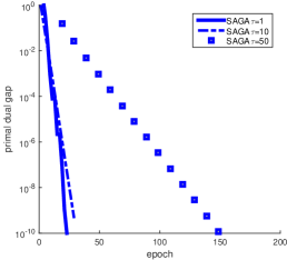
(a) SAGA; ijcnn1

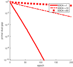
(b) SDCA; ijcnn1

Figure 4: mini-batch SAGA V.S. mini-batch SDCA: ijcnn1

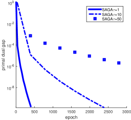
(a) SAGA; a9a

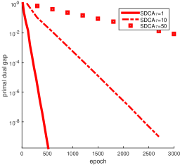
(b) SDCA; a9a

Figure 5: mini-batch SAGA V.S. mini-batch SDCA: a9a

(a) SAGA; w8a

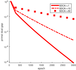
(b) SDCA; w8a

Figure 6: mini-batch SAGA V.S. mini-batch SDCA: w8a

E.2 Importance sampling

We compare uniform sampling SAGA (SAGA-UNI) with importance sampling SAGA (SAGA-IP), as described in Section 3.3 , on three values of $\tau\in\{1,10,50\}$. The results for the datasets w8a, ijcnn1 and a9a are shown in Figure 7. For the dataset ijcnn1, mini-batch with importance sampling almost achieves linear speedup as the number of epochs does not increase with $\tau$. For the dataset w8a, mini-batch with importance sampling can even need less number of epochs than serial uniform sampling. For the dataset a9a, importance sampling slightly but consistently improves over uniform sampling. Note that we adopt the importance sampling strategy described in Hanzely & Richtárik (2019) and the actual running time is the same as uniform sampling.

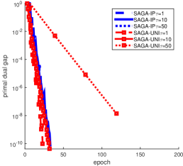
(a) ijcnn1

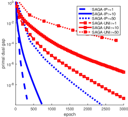
(b) w8a

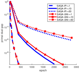
(c) a9a

Figure 7: importance sampling V.S. uniform sampling

E.3 Comparison with Coordinate Descent

We consider the un-regularized logistic regression problem (21) with $\lambda_{1}=\lambda_{2}=0$. In this case, Theorem 4.4 applies and we expect to have linear convergence of SAGA without any knowledge on the constant $\mu$ satsifying Assumption (4.2), see Remark 4.5. This makes SAGA comparable with descent methods such as gradient method and coordinate descent (CD) method. However, comparing with their deterministic counterparts, the speedup provided by CD can be at most of order $d$ while the speedup by SAGA can be of order $n$. Thus SAGA is much preferable than CD when $n$ is larger than $d$. We provide numerical evidence in Figure 8.

(a) ijcnn1

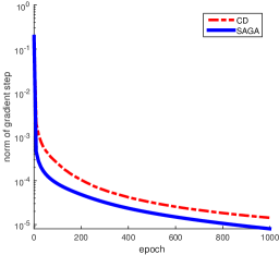
(b) w8a

(c) a9a

Figure 8: SAGA V.S. CD

References

- Bibi et al. (2018) Bibi, A., Sailanbayev, A., Ghanem, B., Gower, R. M., and Richtárik, P. Improving SAGA via a probabilistic interpolation with gradient descent. arXiv: 1806.05633, 2018.
- Chambolle et al. (2017) Chambolle, A., Ehrhardt, M. J., Richtárik, P., and Schönlieb, C. B. Stochastic primal-dual hybrid gradient algorithm with arbitrary sampling and imaging applications. SIAM Journal on Optimization, 28(4):2783–2808, 2017.
- Csiba & Richtárik (2015) Csiba, D. and Richtárik, P. Primal method for ERM with flexible mini-batching schemes and non-convex losses. arXiv:1506.02227, 2015.
- Csiba & Richtárik (2018) Csiba, D. and Richtárik, P. Importance sampling for minibatches. Journal of Machine Learning Research, 19(27):1–21, 2018.
- Defazio et al. (2014) Defazio, A., Bach, F., and Lacoste-Julien, S. SAGA: A fast incremental gradient method with support for non-strongly convex composite objectives. In Ghahramani, Z., Welling, M., Cortes, C., Lawrence, N. D., and Weinberger, K. Q. (eds.), Advances in Neural Information Processing Systems 27, pp. 1646–1654. Curran Associates, Inc., 2014.
- Gower et al. (2018) Gower, R. M., Richtárik, P., and Bach, F. Stochastic quasi-gradient methods: Variance reduction via Jacobian sketching. arXiv Preprint arXiv: 1805.02632, 2018.
- Hanzely & Richtárik (2018) Hanzely, F. and Richtárik, P. Accelerated coordinate descent with arbitrary sampling and best rates for minibatches. arXiv Preprint arXiv: 1809.09354, 2018.
- Hanzely & Richtárik (2019) Hanzely, F. and Richtárik, P. Accelerated coordinate descent with arbitrary sampling and best rates for minibatches. In The 22nd International Conference on Artificial Intelligence and Statistics, 2019.
- Horváth & Richtárik (2018) Horváth, S. and Richtárik, P. Nonconvex variance reduced optimization with arbitrary sampling. arXiv:1809.04146, 2018.
- Johnson & Zhang (2013) Johnson, R. and Zhang, T. Accelerating stochastic gradient descent using predictive variance reduction. In NIPS, pp. 315–323, 2013.
- Konečný & Richtárik (2017) Konečný, J. and Richtárik, P. Semi-stochastic gradient descent methods. Frontiers in Applied Mathematics and Statistics, pp. 1–14, 2017. URL http://arxiv.org/abs/1312.1666.
- Konečný et al. (2016) Konečný, J., Lu, J., Richtárik, P., and Takáč, M. Mini-batch semi-stochastic gradient descent in the proximal setting. IEEE Journal of Selected Topics in Signal Processing, 10(2):242–255, 2016.
- Loizou & Richtárik (2017a) Loizou, N. and Richtárik, P. Linearly convergent stochastic heavy ball method for minimizing generalization error. In NIPS Workshop on Optimization for Machine Learning, 2017a.
- Loizou & Richtárik (2017b) Loizou, N. and Richtárik, P. Momentum and stochastic momentum for stochastic gradient, Newton, proximal point and subspace descent methods. arXiv:1712.09677, 2017b.
- Mairal (2015) Mairal, J. Incremental majorization-minimization optimization with application to large-scale machine learning. SIAM Journal on Optimization, 25(2):829–855, 2015. URL http://jmlr.org/papers/volume16/mokhtari15a/mokhtari15a.pdf.
- Necoara et al. (2018) Necoara, I., Nesterov, Y., and Glineur, F. Linear convergence of first order methods for non-strongly convex optimization. Mathematical Programming, pp. 1–39, 2018. doi: https://doi.org/10.1007/s10107-018-1232-1.
- Needell et al. (2015) Needell, D., Srebro, N., and Ward, R. Stochastic gradient descent, weighted sampling, and the randomized Kaczmarz algorithm. Mathematical Programming, 2015.
- Nemirovski et al. (2009) Nemirovski, A., Juditsky, A., Lan, G., and Shapiro, A. Robust stochastic approximation approach to stochastic programming. SIAM Journal on Optimization, 19(4):1574–1609, 2009.
- Poon et al. (2018) Poon, C., Liang, J., and Schönlieb, C. Local convergence properties of SAGA/Prox-SVRG and acceleration. In Dy, J. and Krause, A. (eds.), Proceedings of the 35th International Conference on Machine Learning, volume 80 of Proceedings of Machine Learning Research, pp. 4124–4132, Stockholmsmässan, Stockholm Sweden, 10–15 Jul 2018. PMLR.
- Qu & Richtárik (2016a) Qu, Z. and Richtárik, P. Coordinate descent with arbitrary sampling I: Algorithms and complexity. Optimization Methods and Software, 31(5):829–857, 2016a.
- Qu & Richtárik (2016b) Qu, Z. and Richtárik, P. Coordinate descent with arbitrary sampling II: Expected separable overapproximation. Optimization Methods and Software, 31(5):858–884, 2016b.
- Qu et al. (2015) Qu, Z., Richtárik, P., and Zhang, T. Quartz: Randomized dual coordinate ascent with arbitrary sampling. In Cortes, C., Lawrence, N. D., Lee, D. D., Sugiyama, M., and Garnett, R. (eds.), Advances in Neural Information Processing Systems 28, pp. 865–873. Curran Associates, Inc., 2015.
- Richtárik & Takáč (2016) Richtárik, P. and Takáč, M. On optimal probabilities in stochastic coordinate descent methods. Optimization Letters, 10(6):1233–1243, 2016.
- Richtárik & Takáč (2014) Richtárik, P. and Takáč, M. Iteration complexity of randomized block-coordinate descent methods for minimizing a composite function. Mathematical Programming, 144(2):1–38, 2014.
- Richtárik & Takáč (2016) Richtárik, P. and Takáč, M. Parallel coordinate descent methods for big data optimization. Mathematical Programming, 156(1-2):433–484, 2016.
- Robbins & Monro (1951) Robbins, H. and Monro, S. A stochastic approximation method. Annals of Mathematical Statistics, 22:400–407, 1951.
- Schmidt et al. (2015) Schmidt, M., Babanezhad, R., Ahmed, M. O., Defazio, A., Clifton, A., and Sarkar, A. Non-uniform stochastic average gradient method for training conditional random fields. In 18th International Conference on Artificial Intelligence and Statistics, 2015.
- Schmidt et al. (2017) Schmidt, M., Le Roux, N., and Bach, F. Minimizing finite sums with the stochastic average gradient. Math. Program., 162(1-2):83–112, 2017.
- Shalev-Shwartz (2016) Shalev-Shwartz, S. SDCA without duality, regularization, and individual convexity. In Proceedings of The 33rd International Conference on Machine Learning, volume 48, pp. 747–754, 2016.
- Shalev-Shwartz & Ben-David (2014) Shalev-Shwartz, S. and Ben-David, S. Understanding machine learning: from theory to algorithms. Cambridge University Press, 2014.
- Shalev-Shwartz & Zhang (2013) Shalev-Shwartz, S. and Zhang, T. Stochastic dual coordinate ascent methods for regularized loss. Journal of Machine Learning Research, 14(1):567–599, 2013.
- Takáč et al. (2013) Takáč, M., Bijral, A., Richtárik, P., and Srebro, N. Mini-batch primal and dual methods for SVMs. In 30th International Conference on Machine Learning, pp. 537–552, 2013.
- Xiao & Zhang (2014a) Xiao, L. and Zhang, T. A proximal stochastic gradient method with progressive variance reduction. SIAM Journal on Optimization, 24(4):2057–2075, 2014a. doi: 10.1137/140961791.
- Xiao & Zhang (2014b) Xiao, L. and Zhang, T. A proximal stochastic gradient method with progressive variance reduction. SIAM Journal on Optimization, 24(4):2057–2075, 2014b.
- Xu et al. (2017) Xu, Y., Lin, Q., and Yang, T. Adaptive svrg methods under error bound conditions with unknown growth parameter. In Guyon, I., Luxburg, U. V., Bengio, S., Wallach, H., Fergus, R., Vishwanathan, S., and Garnett, R. (eds.), Advances in Neural Information Processing Systems 30, pp. 3277–3287. Curran Associates, Inc., 2017.
- Zhang & Lin (2015) Zhang, Y. and Lin, X. Stochastic primal-dual coordinate method for regularized empirical risk minimization. In Blei, D. and Bach, F. (eds.), Proceedings of the 32nd International Conference on Machine Learning (ICML-15), pp. 353–361. JMLR Workshop and Conference Proceedings, 2015. URL http://jmlr.org/proceedings/papers/v37/zhanga15.pdf.
- Zhao & Zhang (2015) Zhao, P. and Zhang, T. Stochastic optimization with importance sampling. The 32nd International Conference on Machine Learning, 37:1–9, 2015.