Fairness risk measures

Abstract

Ensuring that classifiers are non-discriminatory or fair with respect to a sensitive feature (e.g., race or gender) is a topical problem. Progress in this task requires fixing a definition of fairness, and there have been several proposals in this regard over the past few years. Several of these, however, assume either binary sensitive features (thus precluding categorical or real-valued sensitive groups), or result in non-convex objectives (thus adversely affecting the optimisation landscape).

In this paper, we propose a new definition of fairness that generalises some existing proposals, while allowing for generic sensitive features and resulting in a convex objective. The key idea is to enforce that the expected losses (or risks) across each subgroup induced by the sensitive feature are commensurate. We show how this relates to the rich literature on risk measures from mathematical finance. As a special case, this leads to a new convex fairness-aware objective based on minimising the conditional value at risk (CVaR).

1 Introduction

Ensuring that learned classifiers are non-discriminatory or fair with respect to some sensitive feature (e.g., race or gender) is a topical problem (Pedreshi et al., 2008; Žliobaitė, 2017; Chouldechova et al., 2018). Progress on this problem requires that one agrees upon some pre-defined notion of fairness; to this end, there have been several definitions of fairness at both the individual (Dwork et al., 2012; Kusner et al., 2017; Speicher et al., 2018) and group level (Calders and Verwer, 2010; Feldman et al., 2015; Hardt et al., 2016; Zafar et al., 2017b; Heidari et al., 2019).

Recently, several works (Zafar et al., 2017b; Dwork et al., 2018; Hashimoto et al., 2018; Alabi et al., 2018; Speicher et al., 2018; Donini et al., 2018; Heidari et al., 2019) have abstracted earlier definitions of fairness by framing the problem in terms of subgroup losses. Intuitively, these works posit that a fair predictor incurs similar losses for each sensitive feature subgroup (e.g., men and women). One encourages fairness by minimising specific notions of disparity of subgroup losses. For specific choices of loss, this leads to a convex objective (Zafar et al., 2017c; Donini et al., 2018).

In this paper, we propose a new definition of fairness that follows this theme, but abstracts the notion of subgroup loss disparity. Our resulting framework is applicable for generic convex base losses (e.g., hinge), complex sensitive features (e.g., multi-valued), and results in a convex objective. In detail, our contributions are as follows:

• building on notions of fairness in terms of subgroup errors (Zafar et al., 2017b; Dwork et al., 2018; Donini et al., 2018), we provide a new definition of fairness (Definition 3) requiring the average losses (or risks) for each sensitive feature subgroup have low deviation.

• we draw a connection (Corollary 12) between our proposed definition of fairness and the rich literature on risk measures from mathematical finance (Artzner et al., 1999; Föllmer and Schied, 2011), thus allowing one to leverage tools and analyses from the latter.

• we propose a new convex fairness-aware objective (Equation 26) based on minimising the conditional value at risk (CVaR) (Rockafellar and Uryasev, 2000), and relate it to existing learning objectives.

In a nutshell, our proposal is to break up the standard risk into risks on each subgroup defined by the sensitive feature. We combine these via an aggregator which measures the mean and deviation of the subgroup risks. By defining some axioms an aggregator should satisfy, we obtain a connection to risk measures from finance and operations research.

We remark that much of the work in the paper is in setting up the problem to easily exploit a wide body of existing results on risk measures; however, to our knowledge, the application of such tools to fairness is novel. The end result is a simple, powerful framework to learn fair classifiers.

In the sequel, after reviewing existing work (§2), we introduce our new definition of fairness (§3), and relate it to financial risk measures (§4). We detail a special case employing the conditional value at risk (§5), further develop our approach (§6), and confirm its empirical viability (§7).

2 Background

We briefly review the fairness-aware learning problem.

2.1 Standard and fairness-aware learning

Given pairs of instances (e.g., job applicants) and target labels (e.g., likelihood of repaying a loan), supervised learning concerns finding a predictor that best estimates the target label for new instances. Formally, suppose there is a feature set $X$, and label set $Y$. A predictor is any $f\colon X\to A$ for some action set $A$, where typically $A=Y$. Suppose we are given a class of predictors $\mathscr{F}\subseteq A^{X}$, and a loss function $\ell\colon Y\times A\rightarrow\mathbb{R}_{\geq 0}$ measuring the disagreement between a target label and its prediction. The base goal of learning is to find an $f^{*}\in\mathscr{F}$ minimising the risk or expected loss:

$$f^{*}=\underset{f\in\mathscr{F}}{\operatornamewithlimits{argmin}}\,L(f)\text{ where }L(f):=\underset{\mathsf{X},\mathsf{Y}}{\mathbb{E}}\left[\ell(\mathsf{Y},f(\mathsf{X}))\right],$$ (1)

where $\mathsf{X},\mathsf{Y}$ are drawn from some distribution over $X\times Y$.

In fairness-aware learning, we augment the base goal by requiring our predictor does not discriminate with respect to some sensitive feature (e.g., race). Formally, suppose there is a sensitive set $S$ over which there is a random variable $\mathsf{S}$, and that the feature set $X$ contains $S$ as a subset. A fairness measure is some $\Lambda(\cdot)$ for which $\Lambda(\mathsf{Y},f(\mathsf{X}),\mathsf{S})$ evaluates the level of discrimination of $f$. The fairness goal is to find an $f$ minimising the risk subject to $\Lambda$ being small: for $\epsilon\geq 0$,

$$f^{*}=\underset{f\in\mathscr{F}}{\operatornamewithlimits{argmin}}\,L(f)\text{ such that }\Lambda(\mathsf{Y},f(\mathsf{X}),\mathsf{S})\leq\epsilon.$$ (2)

2.2 Measures of perfect fairness

To design a fairness measure $\Lambda$, it is useful to decide what it means for a predictor to be perfectly fair. Most formalisms of perfect (group) fairness are statements of statistical independence. Demographic parity (Dwork et al., 2012) requires

$$\mathsf{A}\mathchoice{\mathrel{\hbox to0.0pt{$\displaystyle\perp$\hss}\mkern 2.0mu{\displaystyle\perp}}}{\mathrel{\hbox to0.0pt{$\textstyle\perp$\hss}\mkern 2.0mu{\textstyle\perp}}}{\mathrel{\hbox to0.0pt{$\scriptstyle\perp$\hss}\mkern 2.0mu{\scriptstyle\perp}}}{\mathrel{\hbox to0.0pt{$\scriptscriptstyle\perp$\hss}\mkern 2.0mu{\scriptscriptstyle\perp}}}\mathsf{S},$$ (3)

so that knowledge of the predictions $\mathsf{A}:=f(\mathsf{X})$ provides no knowledge of the sensitive feature $\mathsf{S}$. For example, when $S=\{{\tt male},{\tt female}\}$, this would mean that the distribution of predictions are identical for both men and women. On the other hand, equalised odds (Hardt et al., 2016) requires

$$\mathsf{A}\mathchoice{\mathrel{\hbox to0.0pt{$\displaystyle\perp$\hss}\mkern 2.0mu{\displaystyle\perp}}}{\mathrel{\hbox to0.0pt{$\textstyle\perp$\hss}\mkern 2.0mu{\textstyle\perp}}}{\mathrel{\hbox to0.0pt{$\scriptstyle\perp$\hss}\mkern 2.0mu{\scriptstyle\perp}}}{\mathrel{\hbox to0.0pt{$\scriptscriptstyle\perp$\hss}\mkern 2.0mu{\scriptscriptstyle\perp}}}\mathsf{S}\mid\mathsf{Y},$$ (4)

so that given knowledge of the true label $\mathsf{Y}$, knowledge of the predictions $\mathsf{A}$ provides no knowledge of the sensitive feature $\mathsf{S}$. Continuing the previous example, this requires that the predictions do not discriminate between men and women beyond whatever power these have in predicting $\mathsf{Y}$. Similarly, lack of disparate mistreatment (Zafar et al., 2017b) constrains the subgroup error rates to be identical:

$$(\forall s,s^{\prime}\in S)\,\mathbb{P}(\mathsf{Y}\neq\mathsf{A}\mid\mathsf{S}=s)=\mathbb{P}(\mathsf{Y}\neq\mathsf{A}\mid\mathsf{S}=s^{\prime}).$$ (5)

There are other extant notions of perfect fairness (Zafar et al., 2017a; Ritov et al., 2017; Heidari et al., 2018; Zhang and Bareinboim, 2018), including those for individual rather than group fairness (Dwork et al., 2012; Kusner et al., 2017).

2.3 Measures of approximate fairness

Notions of perfect fairness represent ideal statements about the world. When learning a classifier from a finite training sample, it is infeasible to guarantee perfect fairness on a test sample (Agarwal et al., 2018). In practice, one often instead works instead with measures of approximate fairness. The learner may then seek to achieve a tradeoff between fairness and accuracy (Menon and Williamson, 2018).

We highlight three popular measures of approximate fairness, using demographic parity (3) as the underlying perfect fairness notion for simplicity. The first is to look at the maximal deviation between subgroup predictions (Calmon et al., 2017), (Alabi et al., 2018, Section 5.2.2):

$$\Lambda_{\mathrm{dev}}(\mathsf{A},\mathsf{S})=\sup_{a,s,s^{\prime}}|\mathbb{P}(\mathsf{A}=a\mid\mathsf{S}=s)-\mathbb{P}(\mathsf{A}=a\mid\mathsf{S}=s^{\prime})|.$$

This measure is popular for binary $S$, where it is known as the mean difference score (Calders and Verwer, 2010). However, it involves computing $|S|^{2}$ terms for categorical $S$, and is infeasible for real-valued $S$. The former issue can be addressed with a simple variant (Agarwal et al., 2018).

An elegant alternative is to recall that perfect fairness measures assert that certain random variables are independent. One may naturally measure approximate fairness by measuring their degree of independence. For example, one might quantify approximate demographic parity (3) via

$$\Lambda_{\mathrm{MI}}(\mathsf{A},\mathsf{S})=\mathrm{MI}(\mathsf{A};\mathsf{S})=\mathrm{KL}(\mathbb{P}(\mathsf{A},\mathsf{S})\,\|\,\mathbb{P}(\mathsf{A})\cdot\mathbb{P}(\mathsf{S})),$$ (6)

where $\mathrm{MI}$ denotes the mutual information, $\mathrm{KL}$ the Kullback-Leibler divergence, $\mathbb{P}(\mathsf{A},\mathsf{S})$ the joint distribution over predictions and sensitive features, and $\mathbb{P}(\mathsf{A})$, $\mathbb{P}(\mathsf{S})$ the corresponding marginals. Since the MI measures the degree of independence of two random variables, $\Lambda_{\mathrm{MI}}$ is a natural measure of approximate demographic parity (Kamishima et al., 2012; Fukuchi et al., 2013; Calmon et al., 2017; Ghassami et al., 2018). One can replace the KL divergence in (6) with other measures of dissimilarity between distributions, e.g., an $f$-divergence (Komiyama and Shimao, 2017) or Hilbert-Schmidt criterion (Pérez-Suay et al., 2017).

Conceptually, measures based on (6) have appealing generality: in particular, they can seamlessly handle multi-class, multi-label and continuous $S$. However, they typically result in a non-convex objective (Kamishima et al., 2012). An alternate measure that is similarly general, but convex, is the covariance between the target and sensitive features (Zafar et al., 2017c; Olfat and Aswani, 2018; Donini et al., 2018):

$$\Lambda_{\mathrm{cov}}(\mathsf{A},\mathsf{S})=\mathrm{Cov}(\mathsf{A},\mathsf{S})=\mathbb{E}[\mathsf{A}\cdot\mathsf{S}]-\mathbb{E}[\mathsf{A}]\cdot\mathbb{E}[\mathsf{S}].$$ (7)

2.4 Fairness-aware algorithms

Having fixed a notion of perfect or approximate fairness, one may then go about designing a fairness-aware learning algorithm. Broadly, these follow one of three approaches:

1. pre-process the training set to ensure fairness of any learned model (Zemel et al., 2013; Johndrow and Lum, 2017; Calmon et al., 2017; Adler et al., 2018; del Barrio et al., 2018; McNamara et al., 2019);

2. post-process model predictions to ensure their fairness (Feldman et al., 2015; Hardt et al., 2016);

3. directly ensure fairness by optimising (2) (Zafar et al., 2016, 2017b; Agarwal et al., 2018; Donini et al., 2018).

This paper focusses on methods of type (c); we defer implications for methods of types (a) and (b) to future work.

2.5 Scope of this paper

In relation to the above (necessarily incomplete) survey, the scope of the present work is in providing:

1. a new notion of approximate fairness (Definition 3),

2. a new method that optimises for this notion (§5), and

3. a new connection between fairness and concepts from mathematical finance (Corollary 12).

In more detail, we consider fairness in terms of subgroup risk, following (Zafar et al., 2017b; Donini et al., 2018; Dwork et al., 2018; Alabi et al., 2018). Our new notion of approximate fairness is that these risks exhibit low deviation. By connecting this to risk measures in mathematical finance, we arrive at a convex objective for fairness-aware learning, applicable for generic sensitive features $S$, and with interesting connections to some existing learning paradigms.

3 Fairness as subgroup risk deviation

We present our new measure of fairness by introducing the notion of subgroup risks, and using it to define natural measures of perfect (§3.2) and approximate fairness (§3.3). We also define some recurring notation, summarised in Table 1. The core idea of our proposal is to aggregate the subgroup risks by measuring their mean behaviour and deviance (Equations 14 and 15).

Symbol	Meaning
$\ell,f$	Base loss, predictor
$L(f)$	Risk of $f$ on entire population
$L_{s}(f)$	Risk of $f$ on subgroup with $S=s$
$\mathsf{L}(f)$	Random variable of all subgroup risks
$\mathcal{D}(\mathsf{L}(f))$	Deviation of subgroup risks
$\mathcal{R}(\mathsf{L}(f))$	Aggregation of subgroup risks

Table 1: Glossary of important symbols.

3.1 Subgroup risks

Observe that the sensitive feature $S$ partitions the instance space $X$ into subgroups (e.g., men and women). It will be useful to define two induced quantities. The first is the subgroup risk for a predictor $f$, which for any $s\in S$ is

$$L_{s}(f):=\underset{\mathsf{X},\mathsf{Y}|\mathsf{S}=s}{\mathbb{E}}\ell(\mathsf{Y},f(\mathsf{X})).$$ (8)

The second is the random variable $\mathsf{L}(f):=L_{\mathsf{S}}(f)$ summarising all subgroup risks. For $|S|<\infty$, this is simply a discrete random variable taking on $|S|$ possible values, i.e., $\{L_{s}(f)\}_{s\in S}$, with corresponding probabilities $\mathbb{P}(\mathsf{S}=s)$.

We can now rewrite the original risk $L(f)$ from (1) as an average over these subgroup risks:

$$L(f)=\underset{\mathsf{S}}{\mathbb{E}}\,\underset{\mathsf{X},\mathsf{Y}\mid\mathsf{S}}{\mathbb{E}}[\ell(\mathsf{Y},f(\mathsf{X}))]=\mathbb{E}[\mathsf{L}(f)].$$ (9)

The base goal of learning (1) is thus expressible as

$$f^{*}=\underset{f\in\mathscr{F}}{\operatorname{argmin}}\,{\mathbb{E}}[\mathsf{L}(f)],$$ (10)

so that one seeks good average subgroup risk. Equally, we wish to select $f^{*}\in\mathscr{F}$ based on the expectations of the family of random variables $\{\mathsf{L}(f)\}_{f\in\mathscr{F}}$.

We now introduce our new measure of fairness. Following the discussion in §2, we do so in two steps: we start by settling on a notion of perfect fairness based on the subgroup risks, and then present an approximate version of the same.

3.2 Perfect fairness via subgroup risks

Every measure of fairness in §2.2 specifies that our predictor $f$ behaves similarly across the sub-groups induced by $S$. We employ a notion of perfect fairness that is faithful to this.

Definition 1.

We say that a predictor $f\in\mathscr{F}$ is perfectly fair with respect to $\ell$ if all subgroups attain the same average loss; i.e., $\mathsf{L}(f)$ is a constant random variable, so that

$$(\forall s,s^{\prime}\in S)\,\underset{\mathsf{X},\mathsf{Y}|\mathsf{S}=s}{\mathbb{E}}\ell(\mathsf{Y},f(\mathsf{X}))=\underset{{\mathsf{X},\mathsf{Y}|\mathsf{S}=s^{\prime}}}{\mathbb{E}}\ell(\mathsf{Y},f(\mathsf{X})).$$ (11)

Abstractly, the idea behind (11) is that the loss $\ell$ should ideally be chosen to capture all aspects of the problem ignoring fairness; perfect fairness means that regardless of the value of sensitive attribute, the performance does not vary. For a specific choice of $\ell$, Definition 1 captures an existing notion of perfect fairness owing to Zafar et al. (2017b).

Example 2.

For the zero-one loss $\ell_{01}(y,f)=\llbracket y\neq f\rrbracket$, (11) reduces to the previously introduced (5):

$$(\forall s,s^{\prime}\in S)\,\mathbb{P}(f(\mathsf{X})\neq\mathsf{Y}\mid\mathsf{S}=s)=\mathbb{P}(f(\mathsf{X})\neq\mathsf{Y}\mid\mathsf{S}=s^{\prime}).$$

Definition 1 is not new as a measure of perfect fairness. Indeed, Donini et al. (2018, Appendix H) considered essentially the same notion, with additional conditioning on $\mathsf{Y}=1$. Several other recent works implicitly define perfect fairness in terms of subgroup risks (Dwork et al., 2018; Hashimoto et al., 2018; Alabi et al., 2018). Further, recent welfare-based notions of fairness (Speicher et al., 2018; Heidari et al., 2019) also posit that fair classifiers have equally distributed benefit (i.e., negative losses).

However, we build on Definition 1 to provide a novel notion of approximate fairness, one which has appealing properties and provides a bridge to the tools of financial risk measures.

3.3 Approximate fairness via subgroup deviations

A natural way to design an approximate fairness measure based on (11) is to ensure that the subgroup risks $\mathsf{L}(f)$ are roughly constant. Formally, for some deviation measure $\mathcal{D}$ of the non-constancy of a random variable (e.g., the standard deviation), we will require that $\mathcal{D}(\mathsf{L}(f))$ is small.

Definition 3.

Let $\mathcal{D}(\cdot)$ be a measure of deviation of a random variable. For any $\epsilon>0$, we say that $f\in\mathscr{F}$ is $\epsilon$-approximately fair with respect to $\mathcal{D}$ and $\ell$ if the average subgroup losses have small deviation; i.e., $\mathcal{D}(\mathsf{L}(f))<\epsilon$.

Definition 3 is applicable for generic $S$ (e.g., real-valued). For the case of binary $S$, it is consistent with existing notions of approximate fairness, as we now illustrate.

Example 4.

Suppose $S=\{0,1\}$, and that we use deviation measure $\mathcal{D}_{\mathrm{SD}}(\cdot)=\sigma(\cdot)$, where $\sigma$ is the standard deviation of a random variable. Fix $f\in\mathscr{F}$, and for brevity write the subgroup risks as $L_{s}:=L_{s}(f)$ and $\mathsf{L}:=\mathsf{L}(f)$. We have

$$\mathcal{D}_{\mathrm{SD}}(\mathsf{L}) =\sqrt{\mathbb{E}(\mathsf{L}^{2})-\mathbb{E}^{2}(\mathsf{L})}=\frac{1}{2}\cdot|L_{0}-L_{1}|.$$ (12)

Recall that the subgroup risks $L_{s}$ depend on the underlying loss $\ell$. Employing the zero-one loss $\ell_{01}$ in (12) yields

$$\mathcal{D}_{\mathrm{SD}}(\mathsf{L})=\frac{1}{2}\cdot|\mathbb{P}(f(\mathsf{X})\neq\mathsf{Y}\mid\mathsf{S}=0)-\mathbb{P}(f(\mathsf{X})\neq\mathsf{Y}\mid\mathsf{S}=1)|,$$

i.e., the mean-difference score (Calders and Verwer, 2010) applied to the lack of disparate mistreatment (5).

3.4 Fairness-aware learning via subgroup aggregation

To achieve approximate fairness according to Definition 3, we may augment the standard expected risk (10) with a penalty term: for suitable $\lambda>0$, we may find

$$f^{*}=\operatornamewithlimits{argmin}_{f\in\mathscr{F}}\,L(f)+\lambda\cdot\mathcal{D}(\mathsf{L}(f)),$$ (13)

so that we find a predictor that predicts the target label, but does so consistently across all subgroups. Observe now that in light of (9), we can succinctly summarise (13) as

We make two observations. First, both standard risk minimisation (10) and  (14) minimise a function of the subgroup risks $\mathsf{L}(f)$; the only difference is the choice of subgroup risk aggregator $\mathcal{R}_{\lambda}$. In (14), we aim to ensure that the subgroup risks are small, and that they are roughly commensurate. Intuitively, the latter ensures that we do not exhibit systematic bias in terms of mispredictions on one of the subgroups.

Second, given a finite sample $\lbag(x_{j},y_{j},s_{j})\rbag_{j=1}^{m}$, one may solve the empirical analogue of (14): we minimise $\mathcal{R}_{\lambda}(\hat{\mathsf{L}}(f))$, where $\hat{\mathsf{L}}$ comprises empirical subgroup risks, i.e., we employ empirical expectations in (8); see, e.g.,  (27).

We make (14) concrete with an example.

Example 5.

For the setting of Example 4, for deviation measure $\mathcal{D}_{\mathrm{SD}}$ we have the fairness-aware objective (14)

$$\mathcal{R}_{\mathrm{SD},\lambda}(\mathsf{L})=\mathbb{E}(\mathsf{L})+\lambda\cdot\mathcal{D}_{\mathrm{SD}}(\mathsf{L})=\mathbb{E}(\mathsf{L})+\frac{\lambda}{2}\cdot|L_{1}-L_{2}|,$$ (16)

so that we ensure that the average subgroup risk is small, and that the two subgroup risks are commensurate.

Remark 6.

For binary $S$, previous methods sharing our notion of perfect fairness (Definition 1) have objectives similar to (16). There is, however, a subtle difference: in (14), we use the same loss $\ell$ to measure the standard risk, and its deviation across subgroups. However, Zafar et al. (2017b); Donini et al. (2018) employ different losses for these two terms. Specifically, they employ a linear loss for the deviation, which corresponds to measuring the covariance between $\mathsf{A}$ and $\mathsf{S}$ per (7). This choice is crucial to ensuring convexity of their objective; we shall see that one can preserve convexity for other $\ell$ by instead modifying $\mathcal{D}$.

Remark 7.

The idea of moving beyond expectations to a general aggregation of the per-instance losses has precedent in learning theory (Chapelle et al., 2001; Maurer and Pontil, 2009) and robust optimisation (Duchi et al., 2016; Gotoh et al., 2018). These encourage the loss deviance across all samples to be small, i.e., effectively, they treat each instance as its own group. Similar connections will also arise in §5.3.

A natural question at this stage is what constitutes a “sensible” choice of deviation measure $\mathcal{D}$. One may of course proceed with intuitively reasonable choices, such as the standard deviation (Example 4); however, we shall now axiomatise the properties we would like any sensible deviation measure to satisfy. This shall lead to an admissible family of fairness risk measures.

4 Fairness risk measures

The proposal of the previous section was boiled down to a simple recipe in (14): rather than minimise the average of the subgroup risks, we minimise a general functional $\mathcal{R}$ of them, which involves an expectation and deviation $\mathcal{D}$. We now axiomatically specify the class of admissible subgroup aggregators $\mathcal{R}$, which will in turn specify the class of admissible deviations $\mathcal{D}$ (Theorem 13).

The technical aspects here are not new; rather, we leverage results in the risk measures literature (particularly Rockafellar and Uryasev (2013)) for a novel application to fairness.

4.1 Fairness risk measures: an axiomatic definition

At this stage, we employ a slight change of terminology: rather than refer to $\mathcal{R}$ as a risk aggregator, we shall refer to it as a risk measure. The reasoning for this change will become evident in the next section.

With this, we define the class of fairness risk measures $\mathcal{R}$ as those satisfying seven simple mathematical axioms. In what follows, let $\mathcal{L}^{2}(S)$ comprise real-valued random variables over $S$ with finite second moment.

Definition 8.

We say $\mathcal{R}\colon\mathcal{L}^{2}(S)\rightarrow\bar{\mathbb{R}}:=\mathbb{R}\cup\{+\infty\}$ is a fairness risk measure if, for any $\mathsf{Z},\mathsf{Z}^{\prime}\in\mathcal{L}^{2}(S)$ and $C\in\mathbb{R}$, it satisfies the following axioms (F1)–(F7):

F1 Convexity

$\mathcal{R}((1-\lambda)\mathsf{Z}+\lambda\mathsf{Z}^{\prime})\leq(1-\lambda)\mathcal{R}(\mathsf{Z})+\lambda\mathcal{R}(\mathsf{Z}^{\prime})$, $\forall\lambda\in(0,1)$.

F2 Positive Homogeneity

$\mathcal{R}(0)=0$, $\mathcal{R}(\lambda\mathsf{Z})=\lambda\mathcal{R}(\mathsf{Z})$ $\forall\lambda>0$.

F3 Monotonicity

$\mathcal{R}(\mathsf{Z})\leq\mathcal{R}(\mathsf{Z}^{\prime})$ if $\mathsf{Z}\leq\mathsf{Z}^{\prime}$ almost surely.

F4 Lower Semicontinuity

$\{\mathsf{Z}\colon\mathcal{R}(\mathsf{Z})\leq C\}$ is closed.

F5 Translation Invariance

$\mathcal{R}(\mathsf{Z}+C)=\mathcal{R}(\mathsf{Z})+C$.

F6 Aversity

$\mathcal{R}(\mathsf{Z})>\mathbb{E}(\mathsf{Z})$ for any non-constant random variable $\mathsf{Z}$.

F7 Law Invariance

$\mathcal{R}(\mathsf{Z})=\mathcal{R}(\mathsf{Z}^{\prime})$ if $\mathbb{P}_{\mathsf{Z}}=\mathbb{P}_{\mathsf{Z}^{\prime}}$.

In Appendix A, we argue why each of these axioms is natural when $\mathcal{R}$ is used per (14) to ensure fairness across subgroups. Here, we highlight the import of two axioms:

Convexity (F1) is desirable because without it, the risk could be decreased by more fine grained partitioning as we now show. F1 and F2 are equivalent to $\mathcal{R}$ being sub-additive and positive homogeneous (Rockafellar and Uryasev, 2013). Suppose $S=\{0,1\}$ and the sensitive feature is determinate and thus induces a partition $(X_{0},X_{1})$ of $X$. Then $\mathsf{L}=\mathsf{L}^{0}+\mathsf{L}^{1}$, where $\mathsf{L}^{i}$ is the restriction of $\mathsf{L}$ to $X_{i}$, so that e.g. $\mathsf{L}^{0}_{s}=\llbracket s=0\rrbracket\cdot\mathbb{P}(\mathsf{S}=0)\cdot\mathsf{L}_{s}$. Now if $\mathcal{R}$ were not convex, it would not be subadditive, and so $\mathcal{R}(\mathsf{L}^{0}+\mathsf{L}^{1})=\mathcal{R}(\mathsf{L})>\mathcal{R}(\mathsf{L}^{0})+\mathcal{R}(\mathsf{L}^{1})$. That is, by splitting into subgroups we could automatically make our risk measure smaller, which is counter to what we wish to achieve.

Convexity is also desirable because, combined with F3, if $f\mapsto L(f)$ is convex, then so is $f\mapsto\mathcal{R}(\mathsf{L}(f))$. Thus, for convex $\ell$ and $\mathscr{F}$, encouraging fairness does not pose an optimisation burden, in contrast to some existing approaches  (Kamishima et al., 2012; Zafar et al., 2016).

Aversity (F6) has a clear justification, as it penalises deviation from perfect fairness (by Definition 1, this corresponds to constant $\mathsf{L}$); this is essential for any fairness measure.

Remark 9.

The subgroup risk aggregator $\mathcal{R}_{\mathrm{SD}}$ corresponding to the standard deviation (16) does not satisfy F1, and thus is not a fairness risk measure. This does not necessarily preclude its use; while Appendix A makes a case that these measures are sensible to use, we do not claim that these are the only legitimate measures. Nonetheless, we now see that a wide class of measures satisfy F1–F7.

4.2 Relation to financial risk measures

In mathematical finance, a risk measure (Artzner et al., 1999) is a quantification of the potential loss associated with a position, i.e., a function $\rho\colon\mathcal{L}^{2}(S)\to\mathbb{R}$ whose input is a random variable, being the possible outcomes for a position. We now show the intimate relationship between fairness risk measures and two classes of risk measures widely studied in finance and operations research (Artzner et al., 1999; Pflug and Romisch, 2007; Krokhmal et al., 2011; Föllmer and Schied, 2011; Rockafellar and Uryasev, 2013). The first class is readily defined in terms of our existing axioms.

Definition 10.

We say $\mathcal{R}\colon\mathcal{L}^{2}(S)\rightarrow\bar{\mathbb{R}}$ is a coherent measure of risk (Artzner et al., 1999) if it satisfies F1 — F5.

The second class requires two additional axioms:

F8 Translation Equivariance

$\mathcal{R}(\mathsf{Z})=C$ for any constant random variable $\mathsf{Z}$ taking value $C\in\mathbb{R}$.

F9 Positivity under non-constancy

$\mathcal{R}(\mathsf{Z})\geq 0$, with equality if and only if $\mathsf{Z}$ is constant.

Equipped with this, we have the following definition.

Definition 11.

We say $\mathcal{R}\colon\mathcal{L}^{2}(S)\rightarrow\bar{\mathbb{R}}$ is a regular measure of risk (Rockafellar and Uryasev, 2013) if it satisfies F1, F4, F6 and F8. Similarly, $\mathcal{D}\colon\mathcal{L}^{2}(S)\rightarrow\bar{\mathbb{R}}$ is a regular measure of deviation if satisfies F1, F4 and F9.

By employing $\mathsf{Z}=0$, (F5 $\land$ F6) $\implies$ F8. This gives a simple relation between fairness and financial risk measures.

Corollary 12.

Every fairness risk measure is a coherent and regular measure of risk satisfying law-invariance.

4.3 Practical implications

Connecting fairness and financial risk measures is not merely of conceptual interest. In particular, Corollary 12 lets us construct fairness risk measures $\mathcal{R}$ given a regular measure of deviation $\mathcal{D}$ via $\mathcal{R}(\mathsf{Z})=\mathbb{E}(\mathsf{Z})+\mathcal{D}(\mathsf{Z})$. This is a consequence of the following quadrangle theorem.

Theorem 13 (Rockafellar and Uryasev (2013)).

The relations

$$\mathcal{R}(\mathsf{Z})=\mathbb{E}(\mathsf{Z})+\mathcal{D}(\mathsf{Z})\text{ and }\mathcal{D}(\mathsf{Z})=\mathcal{R}(\mathsf{Z})-\mathbb{E}(\mathsf{Z})$$ (17)

give a one-to-one correspondence between regular measures of risk $\mathcal{R}$ and regular measures of deviation $\mathcal{D}$. Further, $\mathcal{R}$ is positively homogeneous iff $\mathcal{D}$ is positively homogeneous; and monotonic iff $\mathcal{D}(\mathsf{Z})\leq\sup\mathsf{Z}-\mathbb{E}(\mathsf{Z})$ for all $\mathsf{Z}\in\mathcal{L}^{2}(S)$.

Remark 14.

Using the construction in (17), we arrive at risk aggregators $\mathcal{R}$ that are an expectation plus a deviance $\mathcal{D}$. By contrast, in (13) we applied a scalar $\lambda$ to the deviance. This is equivalent to using a new deviance $\mathcal{D}_{\lambda}:=\lambda\cdot\mathcal{D}$.

Corollary 12 also allows us to import well-studied financial risk measures for use in a fairness context, as we now study.

5 The CVaR-fairness risk measure

We now illustrate a special case of our framework, where we use conditional value of risk (CVaR) to measure subgroup deviation. This is shown to yield a simple objective (Equation 26), and connect to existing learning paradigms.

5.1 CVaR as a fairness risk measure

We first recall the definition of CVaR. For $\alpha\in(0,1)$ and random variable $\mathsf{Z}$, let $q_{\alpha}(\mathsf{Z})$ be the quantile at level $\alpha$. The conditional value at risk is (Rockafellar and Uryasev, 2000)

$$\mathrm{CVaR}_{\alpha}(\mathsf{Z}):=\mathbb{E}(\mathsf{Z}\mid\mathsf{Z}>q_{\alpha}(\mathsf{Z})),$$ (18)

i.e., it measures the tail behaviour of $\mathsf{Z}$. Now define

$$\mathcal{R}_{\mathrm{CV},\alpha}(\mathsf{Z}) :=\mathrm{CVaR}_{\alpha}(\mathsf{Z})$$ (19)

$$\mathcal{D}_{\mathrm{CV},\alpha}(\mathsf{Z}) :=\mathrm{CVaR}_{\alpha}(\mathsf{Z}-\mathbb{E}(\mathsf{Z})).$$ (20)

Intuitively, $\mathcal{D}_{\mathrm{CV},\alpha}$ measures the tail behaviour of $\mathsf{Z}^{\prime}=\mathsf{Z}-\mathbb{E}(\mathsf{Z})$, i.e., how much $\mathsf{Z}$ deviates above its mean.

One has that $\mathcal{R}_{\mathrm{CV},\alpha}$ and $\mathcal{D}_{\mathrm{CV},\alpha}$ are regular, coherent measures of risk and deviation respectively (Rockafellar and Uryasev, 2013). By Theorem 13, one may equally write $\mathcal{D}_{\mathrm{CV},\alpha}(\mathsf{Z})=\mathrm{CVaR}_{\alpha}(\mathsf{Z})-\mathbb{E}(\mathsf{Z})$. Further, $\mathcal{R}_{\mathrm{CV},\alpha}$ is a fairness risk measure with fairness-aware objective (14)

Here, $\alpha\in(0,1)$ is a tuning parameter. From (18), increasing $\alpha$ focusses attention to the most extreme values of $\mathsf{L}(f)$, i.e., the largest subgroup risks. Interestingly, the limiting cases of $\alpha$ yield famous fairness principles. Per Rockafellar (2007, Equation 5.8), as $\alpha\to 1$, (21) becomes

$$\min_{f\in\mathscr{F}}\max_{s\in S}L_{s}(f),$$ (22)

i.e., we seek all subgroup risks to be small, per the maximin principle (Rawls, 1971). As $\alpha\to 0$, (21) becomes

$$\min_{f\in\mathscr{F}}\mathbb{E}_{\mathsf{S}}(L_{\mathsf{S}}(f)),$$

i.e., we seek the average subgroup risks to be small, per the impartial observer principle (Harsanyi, 1977) for uniform $\mathsf{S}$ (see §6.1). To intuit the effect of generic $\alpha\in(0,1)$, suppose $n=|S|<\infty$, and $\mathsf{S}$ has uniform distribution. Then,

$$\mathrm{CVaR}_{\alpha}(\mathsf{L}(f))=\frac{\lambda_{\alpha}}{k_{\alpha}}\sum_{i=1}^{k_{\alpha}}L_{[i]}(f)+(1-\lambda_{\alpha})\cdot L_{[k_{\alpha}+1]}(f),$$ (23)

where $L_{[i]}(f)$ denotes the $i$th largest subgroup risk, $k_{\alpha}:=\lceil n\alpha\rceil$ and $\lambda_{\alpha}$ is a weighting parameter given by Rockafellar and Uryasev (2002, Proposition 8). When $k_{\alpha}$ is an integer,

$$\mathrm{CVaR}_{\alpha}(\mathsf{L}(f))=\frac{1}{k_{\alpha}}\sum_{i=1}^{k_{\alpha}}L_{[i]}(f),$$ (24)

Minimising (21) seeks that the average of the largest subgroup risks is small. This tightens the range of subgroup risks, thus ensuring they are commensurate. Thus, using CVaR as an aggregator (or deviance measure) yields intuitive objectives. We now show these are feasible to optimise.

Remark 15.

The maximal subgroup risk (22) was also considered in Hashimoto et al. (2018), motivated by settings where group identity is unknown. Objectives that interpolate between maximum and average subgroup risk have been proposed, e.g., Alabi et al. (2018, Section 6.1). These are similar in spirit to (23); note however that (23) allows one to choose any $\alpha\in(0,1)$, and thus effectively account for a partial version of the $(k_{\alpha}+1)$th largest subgroup risk.

Remark 16.

Increasing both $\lambda\in(0,\infty)$ and $\alpha\in(0,1)$ in the fairness risk measures $\mathcal{R}_{\mathrm{SD},\lambda}$ (Equation 16) and $\mathcal{R}_{\mathrm{CV},\alpha}$ (Equation 19) penalise variability of subgroup risks $\mathsf{L}(f)$. But the effects are different in detail: large $\lambda$ means strong control on the variance of $\mathsf{L}(f)$, whereas large $\alpha$ means that attention is only paid to the most extreme values of $\mathsf{L}(f)$.

5.2 Optimising CVaR-fairness

Optimisation of quantities based on the CVaR is aided by a variational representation: for any $\alpha\in(0,1)$ and random variable $\mathsf{Z}$, (Rockafellar and Uryasev, 2000, Theorem 1)

$$\mathrm{CVaR}_{\alpha}(\mathsf{Z})=\min_{\rho\in\mathbb{R}}\left\{\rho+\frac{1}{1-\alpha}\cdot\mathbb{E}[\mathsf{Z}-\rho]_{+}\right\}.$$ (25)

Consequently, the CVaR-fairness objective (21) becomes

This is a convex objective when $f\mapsto\mathsf{L}(f)$ is convex (e.g., using a convex base $\ell$ and $\mathscr{F}$). Given a finite sample $\lbag(x_{j},y_{j},s_{j})\rbag_{j=1}^{m}$ with $n=|S|<+\infty$, this becomes

$$\min_{f\in\mathscr{F},\rho\in\mathbb{R}}\left\{\rho+\frac{1}{n\cdot(1-\alpha)}\sum_{s\in S}\left[\frac{1}{m_{s}}\sum_{j\colon s_{j}=s}\ell(y_{j},f(x_{j}))-\rho\right]_{+}\right\},$$ (27)

for $m_{s}$ the number of examples with sensitive feature $s$. In words, for fixed $\rho$, we find a predictor $f\in\mathscr{F}$ which minimises a variant of the standard expected risk, wherein we discard all subgroup risks which are smaller than $\rho$; i.e., we focus attention on the “hard” subgroups.

5.3 Relation to existing paradigms

Fan et al. (2017) considered the problem of learning a robust binary classifier given a sample $\lbag(x_{j},y_{j})\rbag_{j=1}^{m}$ and loss $\ell\colon Y\times A\to\mathbb{R}$. To achieve this, it was proposed to minimise the average of the top-$k$ per-instance losses for $k\ll m$:

$$\min_{f\in\mathscr{F}}\frac{1}{k}\sum_{i=1}^{k}\ell_{[i]}(f),$$ (28)

where $\ell_{[i]}(f)$ is the $i$th largest element of the per-instance losses $[\,\ell(y_{j},f(x_{j}))\,]_{j=1}^{m}$. Following (24), this is equal to

$$\min_{f\in\mathscr{F}}\mathrm{CVaR}_{\alpha_{k}}(\mathsf{L}_{\mathrm{inst}}(f))$$

where ${\alpha_{k}}:={k}/{m}$, and $\mathsf{L}_{\mathrm{inst}}(f)$ is the discrete random variable of per-instance losses, with values $\{\ell(y_{j},f(x_{j})\}_{j=1}^{m}$. Consequently, despite being developed with a wholly different goal in mind, this objective is a special case of our framework where each instance belongs to a separate group.

CVaR also arises in the $\nu$-SVM (Schölkopf et al., 2000), which alternately parametrises the SVM with $\nu\in(0,1)$, and whose objective is expressible as (Gotoh and Takeda, 2005; Takeda and Sugiyama, 2008; Tsyurmasto et al., 2014)

$$\min_{f\in\mathscr{H}}\frac{1}{2}\|f\|_{\mathscr{H}}^{2}+\nu\cdot\mathrm{CVaR}_{1-\nu}(\mathsf{M}(f)),$$

where $\mathsf{M}(f)$ is the random variable of per-instance margins, taking values $[\,-y_{j}\cdot f(x_{j})\,]_{j=1}^{m}$. This is a special case of our framework where each instance belongs to a separate group, and one employs the “linear” loss $\ell(y,f)=-y\cdot f$: while the $\nu$-SVM ignores (or down-weights) any instance with low margin error, we ignore (or down-weight) any subgroup with low average loss.

6 Extensions and discussion

We briefly observe some extensions of our formulation.

6.1 Sensitive feature weighting

In forming our fairness-aware objective (14), we employed the standard risk $L(f)$, which is a weighted sum of the subgroup risks (Equation 9). The default weighting is the underlying sensitive feature distribution. However, one could easily apply different a weighting $\nu_{S}$ to privilege certain groups over others. For $|S|<\infty$, we could define (c.f. (9))

$$L(f;\nu_{S}):=\underset{\mathsf{S}\sim\nu_{S}}{\mathbb{E}}[L_{\mathsf{S}}(f)]=\sum_{s\in S}\nu_{S}(s)\cdot L_{i}(f).$$ (29)

For example, when $S=\{0,1\}$, if one felt that individuals with $s=0$ were more important to treat well, one could simply put a large mass on $1$, e.g. $\nu_{S}(0)=0.9$ and $\nu_{S}(1)=0.1$. The effects of imposing $\mathsf{S}\sim\nu_{S}$ will similarly be reflected in one’s deviation measure $\mathcal{D}(L_{\mathsf{S}}(f))$.

To treat both groups equally in terms of risk, one could alternately choose $\nu_{S}$ to be uniform. This forms the basis for Harsanyi’s principle of justice (Harsanyi, 1977), and would be analogous to the use of the balanced error in classification (Brodersen et al., 2010; Menon et al., 2013).

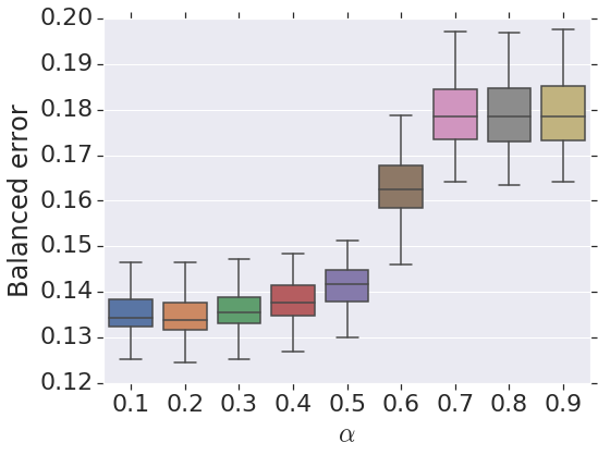
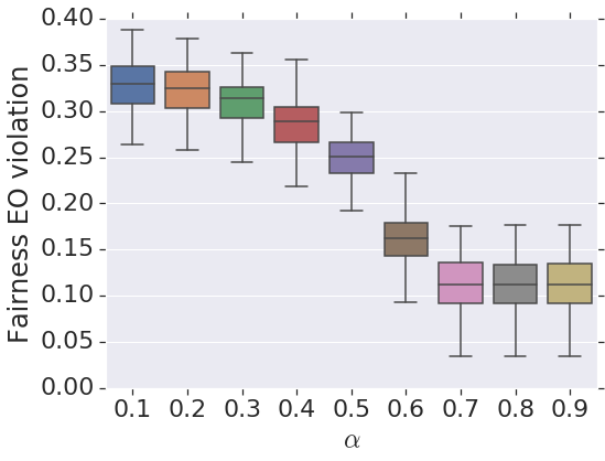
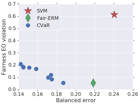
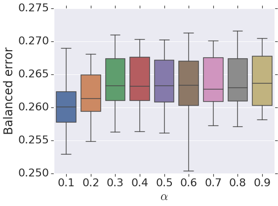
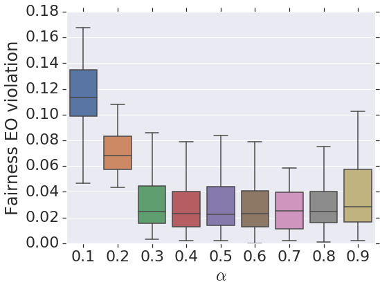
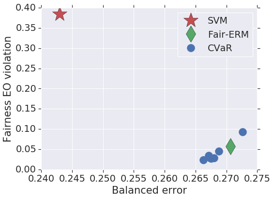
Figure 1: Results on synth (top) and adult (bottom) datasets. The left and middle panel show that as $\alpha$ is varied, CVaR-based optimisation results in a decrease in predictive accuracy and fairness violation. The right panel overlays the performance of CVaR-based optimisation for various $\alpha$ with that of two baselines. The CVaR method is shown to attain a reasonable fairness-accuracy tradeoff.

6.2 Non-binary sensitive features

Our examples thus far have focussed on binary $S$. However, the risk measures underpinning our framework seamlessly handle generic $S$. We make this concrete with two examples. The first is where $S=\mathbb{R}_{\geq 0}$ (as is appropriate for a person’s income, e.g.). Then, for $\alpha\in(0,1)$ and measure $\nu_{S}$ over $S$ per (29), the CVaR-fairness objective (26) is:

$$\min_{f\in\mathscr{F},\rho\in\mathbb{R}}\left\{\rho+\frac{1}{1-\alpha}\cdot\int_{S}[L_{s}(f)-\rho]_{+}\,\nu_{S}(\mathrm{d}s)\right\}.$$ (30)

On a finite sample $\lbag(x_{j},y_{j},s_{j})\rbag_{j=1}^{m}$ with all $s_{j}$’s distinct for simplicity, taking the empirical measure $\hat{\nu}_{S}$ gives

$$\min_{f\in\mathscr{F},\rho\in\mathbb{R}}\left\{\rho+\frac{1}{1-\alpha}\cdot\frac{1}{m}\sum_{j=1}^{m}\left[\ell(y_{j},f(x_{j}))-\rho\right]_{+}\right\},$$ (31)

so that each instance is considered as belonging to the same group. Interestingly, this is equivalent to the top-$k$ objective (28) for $k=m\alpha$. However, one may consider other natural alternatives; e.g., one may construct a non-parametric estimate of $\nu_{S}$ from the given sample, and use this in (30).

The case of multiple sensitive features $\{S_{1},\ldots,S_{l}\}$ can be similarly handled: all one needs to do is define a suitably structured $S$, and a valid measure $\nu_{S}$ over $S$. As an example, one can set $S:=S_{1}\times\cdots\times S_{l}$ and define $\nu_{S}$ as the product of measures $\nu_{S_{i}}$ on each individual sensitive feature.

7 Empirical illustration

We present experiments illustrating the practical viability of our framework. In particular, we demonstrate that optimising the CVaR-fairness objective (27) yields solutions with reasonable fairness-accuracy tradeoffs.

In detail, we assess the performance of CVaR-based optimisation (27) as $\alpha$ is tuned in $\{0.1,0.2,\ldots,0.9\}$. As baselines, we compare against a standard SVM, and the fair-ERM approach of Donini et al. (2018). For all methods, we use square-hinge $\ell(y,f)=[1-yf]_{+}^{2}$ as our base loss, and use regularised linear scorers as our $\mathscr{F}$. We use the validation procedure of Donini et al. (2018), to tune the regularisation strength, but with balanced in place of 0-1 error as the primary measure of predictive performance on $\mathsf{Y}$.

We present results on a synthetic two-dimensional dataset (synth) from Donini et al. (2018), and the UCI adult dataset with gender as the binary $S$. (In Appendix B, we present additional results, including on a real-valued $S$.) For each method, over 100 random 80—20% train-test splits we measure the predictive performance on $\mathsf{Y}$ via the balanced error, and the fairness on $\mathsf{S}$ via the violation of equality of opportunity (EO) (Hardt et al., 2016), as measured by $|\mathbb{P}(\mathsf{A}=1\mid\mathsf{S}=1,\mathsf{Y}=1)-\mathbb{P}(\mathsf{A}=1\mid\mathsf{S}=0,\mathsf{Y}=1)|$. As both datasets are slightly imbalanced, we weight positives and negatives equally for each method.

The left and middle panels of Figure 1 evince that as $\alpha$ is increased, there is a decrease in predictive accuracy accompanied by an increase in fairness (i.e., decreased violation of the EO condition). We remark here that the CVaR method only explicitly encourages the violation with respect to the square-hinge loss is minimised across the subgroups, which is indeed manifest (see Appendix B).

The right panel of Figure 1 summarises the fairness-accuracy tradeoff for all methods on one train-test split. For the CVaR method, we present operating points for all values of $\alpha$. Generally, CVaR’s results are competitive with the fair-ERM approach of Donini et al. (2018). While more extensive experiments are apposite, the above indicates the practical promise in further studying fairness risk measures.

8 Conclusion and future work

We proposed a new definition of fairness that generalises some existing proposals, while allowing for generic sensitive features and resulting in a convex objective. The key idea is to enforce that the expected losses (or risks) across each subgroup induced by the sensitive feature are commensurate. We showed how this relates to the rich literature on risk measures from mathematical finance. As a special case, this leads to a new convex fairness-aware objective based on minimising the conditional value at risk (CVaR).

Our relating of fairness and risk measures motivates study of risk measures beyond CVaR, e.g., spectral measures (Acerbi, 2002), optimised certainty equivalents (Ben-Tal and Teboulle, 2007), & entropic value at risk (Ahmadi-Javid, 2012).

Supplementary material for “Fairness risk measures”

Appendix A Justification of fairness risk measure axioms

We now argue why each of these axioms is natural when $\mathcal{R}$ is used per (14) to ensure fairness across subgroups. We note that apart from (F2), none of these properties can be relaxed without causing problems.

Convexity (F1) is desirable because without it, the risk could be decreased by more fine grained partitioning as we now show. F1 and F2 are equivalent to $\mathcal{R}$ being sub-additive and positive homogeneous [Rockafellar and Uryasev, 2013]. Suppose $S=\{0,1\}$ and the sensitive feature is determinate and thus induces a partition $(X_{0},X_{1})$ of $X$. Then $\mathsf{L}=\mathsf{L}^{0}+\mathsf{L}^{1}$, where $\mathsf{L}^{i}$ is the restriction of $\mathsf{L}$ to $X_{i}$, so that e.g. $\mathsf{L}^{0}_{s}=\llbracket s=0\rrbracket\cdot\mathbb{P}(\mathsf{S}=0)\cdot\mathsf{L}_{s}$. Now if $\mathcal{R}$ were not convex it would not be subadditive and we would have $\mathcal{R}(\mathsf{L}^{0}+\mathsf{L}^{1})=\mathcal{R}(\mathsf{L})>\mathcal{R}(\mathsf{L}^{0})+\mathcal{R}(\mathsf{L}^{1})$. In other words, by splitting into subgroups we could automatically make our risk measure smaller, which is counter to what we wish to achieve. Convexity is also desirable because, combined with F3, it preserves tractability of optimisation.

Positive Homogeneity (F2) is desirable but not essential. We would like our fairness measure to not vary in a manner that changes the optimal $f$ when $\ell$ varies in a manner that leaves the base problem invariant. For example, if $\ell^{\prime}=c\cdot\ell$ for some $c>0$ then obviously $\operatornamewithlimits{argmin}_{f\in\mathscr{F}}L_{\ell}(f)=\operatornamewithlimits{argmin}_{f\in\mathscr{F}}L_{\ell^{\prime}}(f)$. If $\mathcal{R}$ is positively homogeneous, then $\mathcal{R}(\mathsf{L}^{\prime})=\mathcal{R}(c\cdot\mathsf{L})=c\cdot\mathcal{R}(\mathsf{L})$ and thus $\operatornamewithlimits{argmin}_{f\in\mathscr{F}}\mathcal{R}(\mathsf{L})=\operatornamewithlimits{argmin}_{f\in\mathscr{F}}\mathcal{R}(\mathsf{L}^{\prime})$. Observe this last statement would remain true if $\mathcal{R}$ was $k$-homogeneous, for any $k\geq 0$. Whether a relaxation of (F2) adds any practical advantage is not yet understood. Positive homogeneity does imply that the units of measurement of $\mathcal{R}(\mathsf{Z})$ are automatically the same as those for $\mathsf{Z}$. The assumption of 1-homogeneity is also beneficial when analysing duality properties of risk measures; see Rockafellar and Uryasev [2013, Section 6].

Monotonicity (F3) is desirable because when combined with convexity (F1) it ensures that if $f\mapsto L(f)$ is convex, then so will be $f\mapsto\mathcal{R}(\mathsf{L}(f))$; see [Rockafellar and Uryasev, 2013, Section 5], and part 3 of Theorem 13. It is also intuitive that one’s overall risk not increase if all subgroup risks are decreased. We note that a similar monotonicity assumption, and its implications, were also employed in Dwork et al. [2018, Section 4].

Lower Semicontinuity (F4) is a technical assumption that avoids problems with limits [Rockafellar and Uryasev, 2013].

Translation invariance (F5) is desirable because if we replace $\ell$ by $\ell+C$ we have not changed the unfairness at all, just the expected risk value.

Aversity (F6) means that deviation from perfect fairness (Definition 1) is penalised; without this property we would not be capturing deviation from ideal fairness.

Law Invariance (F7) means that $\mathcal{R}$ only depends upon $\mathsf{Z}$ via its distribution $\mathbb{P}_{\mathsf{Z}}$ through an induced functional $\mathcal{F}_{\mathscr{P}}\colon\mathscr{P}(S)\rightarrow\mathbb{R}$. For a fairness measure this would mean that the identity of each of the values of the sensitive feature do not matter, only the distribution of the risk variable $\mathsf{L}(s)$ as a function of $s\in S$. This is clearly a desirable attribute for a fairness measure.

Appendix B Additional experiments

We present some experimental results supplementing those in the body.

B.1 Results with real-valued sensitive feature

We illustrate the viability of using the model with a real-valued sensitive feature $S$. We consider the adult dataset, but this time with fnlwgt (an estimate of how representative an individual is) as the sensitive feature. Following 31, essentially all instances are placed into separate subgroups in forming the CVaR objective. Figure 2 compares the histogram of margin scores $\{y_{i}\cdot f(x_{i})\}_{i=1}^{m}$ for $\alpha=0.1$ and $\alpha=0.9$. We see that, as expected, setting $\alpha=0.9$ encourages all scores to be roughly commensurate.

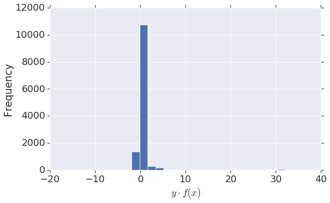
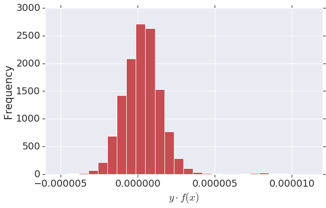
Figure 2: Results on adult dataset with fnlwgt as the continuous sensitive feature. The left and right panel are for $\alpha=0.1$ and $\alpha=0.9$ respectively. Since essentially each individual is a member of a singleton subgroup, the latter is seen to encourage commensurate model predictions, and thus margin scores across all instances.

B.2 Additional results on synth and adult

In Figures 4 and 5, we show the behaviour of the CVaR method as $\alpha$ is varied with respect to different metrics. In Figure 3, we measure the 0-1 error with respect to $\mathsf{Y}$, and the difference of the 0-1 across the subgroups induced by $\mathsf{S}$, i.e., the violation of the demographic parity (DP) condition. Note that since the datasets are slightly imbalanced, the 0-1 error is not ideal as a measure of performance.

To better reflect the nature of class imbalance, in Figure 4, we measure the pairwise disagreement (i.e., one minus the area under the ROC curve) with respect to $\mathsf{Y}$, and the difference of the pairwise disagreement across the subgroups induced by $\mathsf{S}$. In Figure 5, we measure the square hinge loss with respect to $\mathsf{Y}$, and the difference of this loss across the subgroups induced by $\mathsf{S}$. We generally see that, as in the body, increasing $\alpha$ has the effect of reducing predictive accuracy of $\mathsf{Y}$ while also reducing the fairness violation.

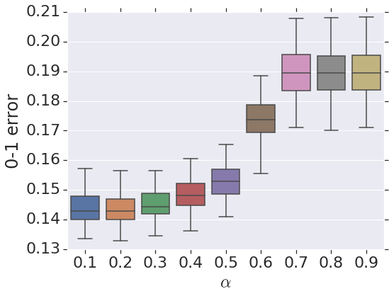
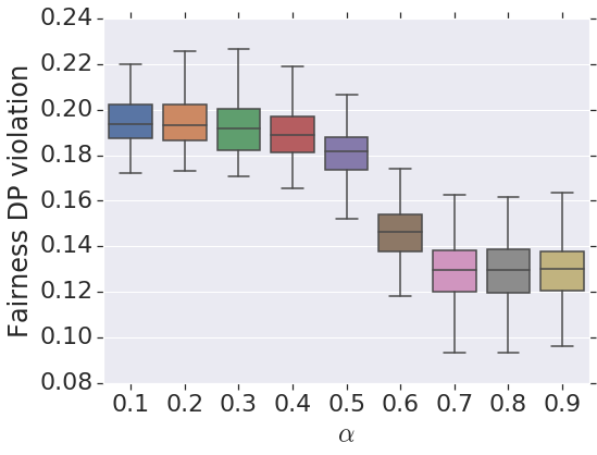
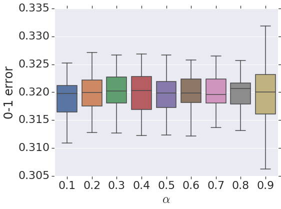
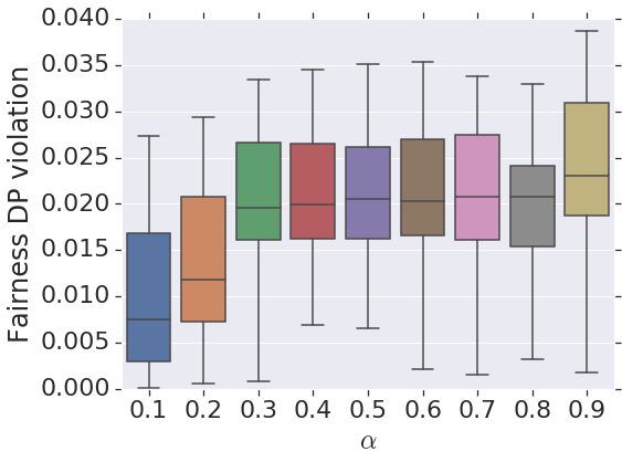
Figure 3: Results on synth (top) and adult (bottom) datasets. The left and right panel show that as $\alpha$ is varied, CVaR-based optimisation generally results in a decrease in predictive accuracy and fairness violation.

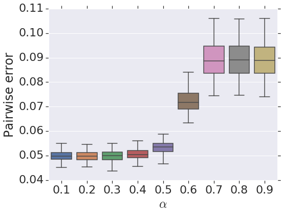
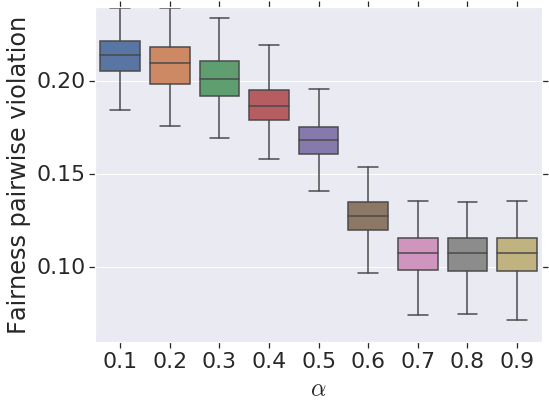
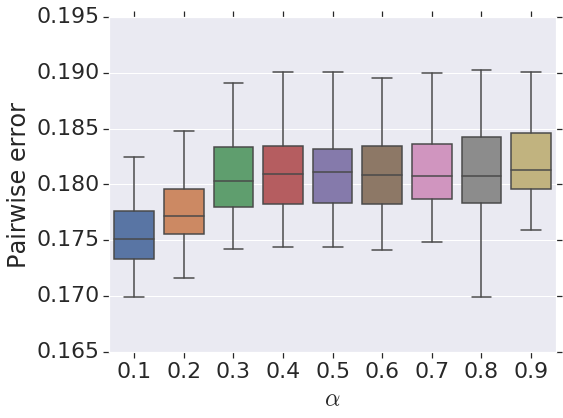
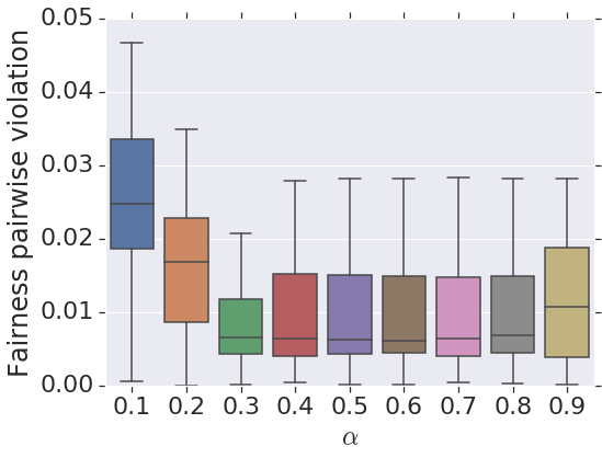
Figure 4: Results on synth (top) and adult (bottom) datasets. The left and right panel show that as $\alpha$ is varied, CVaR-based optimisation generally results in a decrease in predictive accuracy and fairness violation.

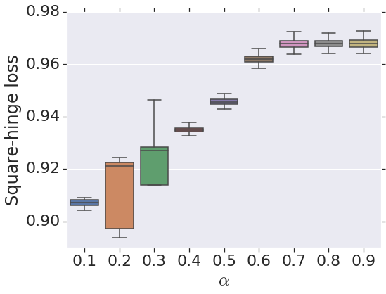
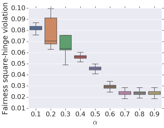
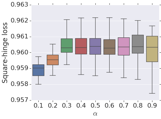
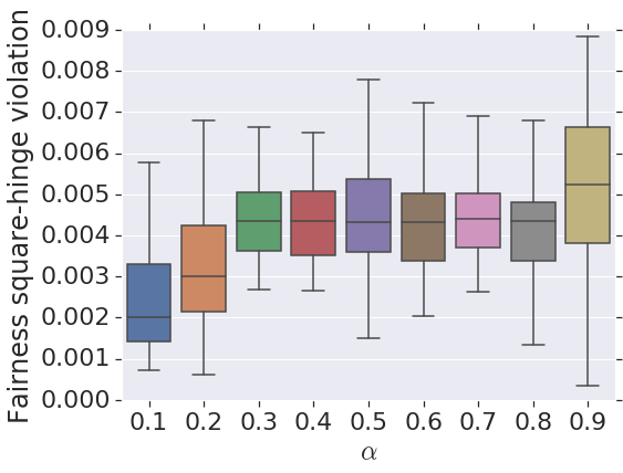
Figure 5: Results on synth (top) and adult (bottom) datasets. The left and right panel show that as $\alpha$ is varied, CVaR-based optimisation generally results in a decrease in predictive accuracy and fairness violation.

References

- Acerbi [2002] Carlo Acerbi. Spectral measures of risk: A coherent representation of subjective risk aversion. Journal of Banking & Finance, 26(7):1505–1518, 2002.
- Adler et al. [2018] Philip Adler, Casey Falk, Sorelle A. Friedler, Tionney Nix, Gabriel Rybeck, Carlos Scheidegger, Brandon Smith, and Suresh Venkatasubramanian. Auditing black-box models for indirect influence. Knowledge and Information Systems, 54(1):95–122, January 2018.
- Agarwal et al. [2018] Alekh Agarwal, Alina Beygelzimer, Miroslav Dudik, John Langford, and Hanna Wallach. A reductions approach to fair classification. In Proceedings of the 35th International Conference on Machine Learning, pages 60–69, 2018.
- Ahmadi-Javid [2012] Amir Ahmadi-Javid. Entropic value-at-risk: A new coherent risk measure. Journal of Optimization Theory and Applications, 155(3):1105–1123, Dec 2012.
- Alabi et al. [2018] Daniel Alabi, Nicole Immorlica, and Adam Tauman Kalai. Unleashing linear optimizers for group-fair learning and optimization. In Proceedings of the 31st Conference On Learning Theory, pages 2043–2066, 06–09 Jul 2018.
- Artzner et al. [1999] Philippe Artzner, Freddy Delbaen, Jean-Marc Eber, and David Heath. Coherent measures of risk. Mathematical finance, 9(3):203–228, 1999.
- Ben-Tal and Teboulle [2007] Aharon Ben-Tal and Marc Teboulle. An old-new concept of convex risk measures: the optimized certainty equivalent. Mathematical Finance, 17(3):449–476, 2007.
- Brodersen et al. [2010] Kay Henning Brodersen, Cheng Soon Ong, Klaas Enno Stephan, and Joachim M. Buhmann. The balanced accuracy and its posterior distribution. In Proceedings of the 20th International Conference on Pattern Recognition, pages 3121–3124, 2010.
- Calders and Verwer [2010] Toon Calders and Sicco Verwer. Three Naive Bayes approaches for discrimination-free classification. Data Mining and Knowledge Discovery, 21(2):277–292, 2010.
- Calmon et al. [2017] Flávio du Pin Calmon, Dennis Wei, Bhanukiran Vinzamuri, Karthikeyan Natesan Ramamurthy, and Kush R. Varshney. Optimized pre-processing for discrimination prevention. In Advances in Neural Information Processing Systems, pages 3995–4004, 2017.
- Chapelle et al. [2001] Olivier Chapelle, Jason Weston, Léon Bottou, and Vladimir Vapnik. Vicinal risk minimization. In Advances in Neural Information Processing Systems 13, pages 416–422. MIT Press, 2001.
- Chouldechova et al. [2018] Alexandra Chouldechova, Diana Benavides Prado, Oleksandr Fialko, and Rhema Vaithianathan. A case study of algorithm-assisted decision making in child maltreatment hotline screening decisions. In Conference on Fairness, Accountability and Transparency, pages 134–148, 2018.
- del Barrio et al. [2018] Eustasio del Barrio, Fabrice Gamboa, Paula Gordaliza, and Jean-Michel Loubes. Obtaining fairness using optimal transport theory. arXiv e-prints, art. arXiv:1806.03195, June 2018.
- Donini et al. [2018] Michele Donini, Luca Oneto, Shai Ben-David, John S Shawe-Taylor, and Massimiliano Pontil. Empirical risk minimization under fairness constraints. In Advances in Neural Information Processing Systems 31, pages 2796–2806. 2018.
- Duchi et al. [2016] John Duchi, Peter Glynn, and Hongseok Namkoong. Statistics of Robust Optimization: A Generalized Empirical Likelihood Approach. arXiv e-prints, art. arXiv:1610.03425, October 2016.
- Dwork et al. [2012] Cynthia Dwork, Moritz Hardt, Toniann Pitassi, Omer Reingold, and Richard Zemel. Fairness through awareness. In Innovations in Theoretical Computer Science Conference, pages 214–226, 2012.
- Dwork et al. [2018] Cynthia Dwork, Nicole Immorlica, Adam Tauman Kalai, and Max Leiserson. Decoupled classifiers for group-fair and efficient machine learning. In Proceedings of the 1st Conference on Fairness, Accountability and Transparency, pages 119–133, 2018.
- Fan et al. [2017] Yanbo Fan, Siwei Lyu, Yiming Ying, and Bao-Gang Hu. Learning with average top-k loss. In Advances in Neural Information Processing Systems, pages 497–505, 2017.
- Feldman et al. [2015] Michael Feldman, Sorelle A. Friedler, John Moeller, Carlos Scheidegger, and Suresh Venkatasubramanian. Certifying and removing disparate impact. In ACM SIGKDD International Conference on Knowledge Discovery and Data Mining (KDD), pages 259–268, 2015.
- Föllmer and Schied [2011] Hans Föllmer and Alexander Schied. Stochastic finance: an introduction in discrete time. Walter de Gruyter, 2011.
- Fukuchi et al. [2013] Kazuto Fukuchi, Jun Sakuma, and Toshihiro Kamishima. Prediction with model-based neutrality. In European Conference on Machine Learning and Knowledge Discovery in Databases, pages 499–514, 2013.
- Ghassami et al. [2018] AmirEmad Ghassami, Sajad Khodadadian, and Negar Kiyavash. Fairness in supervised learning: An information theoretic approach. CoRR, abs/1801.04378, 2018. URL http://arxiv.org/abs/1801.04378.
- Gotoh and Takeda [2005] Jun-ya Gotoh and Akiko Takeda. A linear classification model based on conditional geometric score. Pacific Journal of Optimization, 1:277–296, 2005.
- Gotoh et al. [2018] Jun-ya Gotoh, Michael Jong Kim, and Andrew E.B. Lim. Robust empirical optimization is almost the same as mean-variance optimization. Operations Research Letters, 46(4):448 – 452, 2018.
- Hardt et al. [2016] Moritz Hardt, Eric Price, and Nathan Srebro. Equality of opportunity in supervised learning. In Advances in Neural Information Processing Systems (NIPS), December 2016.
- Harsanyi [1977] John C. Harsanyi. Rational Behaviour and Bargaining Equilibrium in Games and Social Situations. Cambridge University Press, 1977.
- Hashimoto et al. [2018] T. B. Hashimoto, M. Srivastava, H. Namkoong, and P. Liang. Fairness without demographics in repeated loss minimization. In International Conference on Machine Learning, 2018.
- Heidari et al. [2018] Hoda Heidari, Claudio Ferrari, Krishna P. Gummadi, and Andreas Krause. Fairness behind a veil of ignorance: A welfare analysis for automated decision making. In Advances in Neural Information Processing Systems 31, pages 1273–1283, 2018.
- Heidari et al. [2019] Hoda Heidari, Michele Loi, Krishna P. Gummadi, and Andreas Krause. A moral framework for understanding of fair ML through economic models of equality of opportunity. In ACM Conference on Fairness, Accountability, and Transparency, January 2019.
- Johndrow and Lum [2017] James E. Johndrow and Kristian Lum. An algorithm for removing sensitive information: application to race-independent recidivism prediction. arXiv e-prints, art. arXiv:1703.04957, March 2017.
- Kamishima et al. [2012] Toshihiro Kamishima, Shotaro Akaho, Hideki Asoh, and Jun Sakuma. Fairness-aware classifier with prejudice remover regularizer. In European Conference on Machine Learning and Knowledge Discovery in Databases, pages 35–50, 2012.
- Komiyama and Shimao [2017] J. Komiyama and H. Shimao. Two-stage Algorithm for Fairness-aware Machine Learning. ArXiv e-prints, October 2017.
- Krokhmal et al. [2011] Pavlo Krokhmal, Michael Zabarankin, and Stan Uryasev. Modeling and optimization of risk. Surveys in Operations Research and Management Science, 16:49–66, 2011.
- Kusner et al. [2017] Matt J. Kusner, Joshua R. Loftus, Chris Russell, and Ricardo Silva. Counterfactual fairness. In Advances in Neural Information Processing Systems, pages 4069–4079, 2017.
- Maurer and Pontil [2009] Andreas Maurer and Massimiliano Pontil. Empirical bernstein bounds and sample-variance penalization. In COLT, 2009.
- McNamara et al. [2019] Daniel McNamara, Cheng Soon Ong, and Robert C. Williamson. Costs and benefits of fair representation learning. In AAAI Conference on Artificial Intelligence, Ethics and Society, 2019.
- Menon and Williamson [2018] Aditya Krishna Menon and Robert C. Williamson. The cost of fairness in binary classification. In Conference on Fairness, Accountability and Transparency, pages 107–118, 2018.
- Menon et al. [2013] Aditya Krishna Menon, Harikrishna Narasimhan, Shivani Agarwal, and Sanjay Chawla. On the statistical consistency of algorithms for binary classification under class imbalance. In International Conference on Machine Learning (ICML), pages 603–611, 2013.
- Ogryczak and Tamir [2003] Wlodzimierz Ogryczak and Arie Tamir. Minimizing the sum of the k largest functions in linear time. Information Processing Letters, 85(3):117 – 122, 2003.
- Olfat and Aswani [2018] Mahbod Olfat and Anil Aswani. Spectral algorithms for computing fair support vector machines. In International Conference on Artificial Intelligence and Statistics, pages 1933–1942, 2018.
- Pedreshi et al. [2008] Dino Pedreshi, Salvatore Ruggieri, and Franco Turini. Discrimination-aware data mining. In ACM SIGKDD International Conference on Knowledge Discovery and Data Mining (KDD), pages 560–568, 2008.
- Pérez-Suay et al. [2017] Adrián Pérez-Suay, Valero Laparra, Gonzalo Mateo-García, Jordi Muñoz-Marí, Luis Gómez-Chova, and Gustau Camps-Valls. Fair kernel learning. In Machine Learning and Knowledge Discovery in Databases, pages 339–355, 2017.
- Pflug and Romisch [2007] Georg Ch Pflug and Werner Romisch. Modeling, measuring and managing risk. World Scientific, 2007.
- Rawls [1971] John Rawls. A Theory of Justice. Harvard University Press, 1971.
- Ritov et al. [2017] Y. Ritov, Y. Sun, and R. Zhao. On conditional parity as a notion of non-discrimination in machine learning. ArXiv e-prints, June 2017.
- Rockafellar [2007] R. Tyrrell Rockafellar. Coherent approaches to risk in optimization under uncertainty. In OR Tools and Applications: Glimpses of Future Technologies, chapter 3, pages 38–61. 2007.
- Rockafellar and Uryasev [2013] R. Tyrrell Rockafellar and Stan Uryasev. The fundamental risk quadrangle in risk management, optimization and statistical estimation. Surveys in Operations Research and Management Science, 18(1-2):33–53, 2013.
- Rockafellar and Uryasev [2000] R. Tyrrell Rockafellar and Stanislav Uryasev. Optimization of conditional value-at-risk. Journal of Risk, 2:21–41, 2000.
- Rockafellar et al. [2006] R. Tyrrell Rockafellar, Stan Uryasev, and Michael Zabarankin. Generalized deviations in risk analysis. Finance and Stochastics, 10(1):51–74, 2006.
- Rockafellar and Uryasev [2002] R.T. Rockafellar and S. Uryasev. Conditional value-at-risk for general loss distributions. Journal of Banking & Finance, 26(7):1443–1471, 2002.
- Schölkopf et al. [2000] Bernhard Schölkopf, Alex J. Smola, Robert C. Williamson, and Peter L. Bartlett. New support vector algorithms. Neural Computation, 12(5):1207–1245, May 2000.
- Speicher et al. [2018] Till Speicher, Hoda Heidari, Nina Grgic-Hlaca, Krishna P. Gummadi, Adish Singla, Adrian Weller, and Muhammad Bilal Zafar. A unified approach to quantifying algorithmic unfairness: Measuring individual & group unfairness via inequality indices. In Proceedings of the 24th ACM SIGKDD International Conference on Knowledge Discovery & Data Mining, pages 2239–2248, 2018.
- Takeda and Sugiyama [2008] Akiko Takeda and Masashi Sugiyama. nu-support vector machine as conditional value-at-risk minimization. In Proceedings of the Twenty-Fifth International Conference on Machine Learning, pages 1056–1063, 2008.
- Tsyurmasto et al. [2014] Peter Tsyurmasto, Michael Zabarankin, and Stan Uryasev. Value-at-risk support vector machine: stability to outliers. Journal of Combinatorial Optimization, 28(1):218–232, Jul 2014.
- Zafar et al. [2017a] M. B. Zafar, I. Valera, M. Gomez Rodriguez, K. Gummadi, and A. Weller. From parity to preference-based notions of fairness in classification. In Advances in Neural Information Processing Systems 30, pages 229–239, 2017a.
- Zafar et al. [2016] Muhammad Bilal Zafar, Isabel Valera, Manuel Gomez-Rodriguez, and Krishna Gummadi. Learning fair classifiers. arXiv preprint arXiv:1507.05259, 2016.
- Zafar et al. [2017b] Muhammad Bilal Zafar, Isabel Valera, Manuel Gomez-Rodriguez, and Krishna Gummadi. Fairness beyond disparate treatment & disparate impact: Learning classification without disparate mistreatment. In International World Wide Web Conference, 2017b.
- Zafar et al. [2017c] Muhammad Bilal Zafar, Isabel Valera, Manuel Gomez-Rodriguez, and Krishna P. Gummadi. Fairness constraints: Mechanisms for fair classification. In Proceedings of the 20th International Conference on Artificial Intelligence and Statistics, pages 962–970, 2017c.
- Zemel et al. [2013] Richard Zemel, Yu Wu, Kevin Swersky, Toniann Pitassi, and Cynthia Dwork. Learning fair representations. In International Conference on Machine Learning (ICML), 2013.
- Zhang and Bareinboim [2018] Junzhe Zhang and Elias Bareinboim. Equality of opportunity in classification: A causal approach. In Advances in Neural Information Processing Systems 31, pages 3675–3685, 2018.
- Žliobaitė [2017] Indrė Žliobaitė. Measuring discrimination in algorithmic decision making. Data Mining and Knowledge Discovery, 31(4):1060–1089, Jul 2017.