Sparkling nights and very hot days on WASP-18b:
the formation of clouds and the emergence of an ionosphere

Abstract

Context. WASP-18b is an utra-hot Jupiter with a temperature difference of upto 2500K between day and night. Such giant planets begins to emerge as planetary laboratory for understanding cloud formation and gas chemistry in well-tested parameter regimes in order to better understand planetary mass loss and for linking observed element ratios to planet formation and evolution.

Aims. We aim to understand where clouds form, their interaction with the gas phase chemistry through depletion and enrichment, the ionisation of the atmospheric gas and the possible emergence of an ionosphere on ultra-hot Jupiters.

Methods. We utilize 1D profiles from a 3D atmosphere simulations for WASP-18b as input for kinetic cloud formation and gas-phase chemical equilibrium calculations. We solve our kinetic cloud formation model for these 1D profiles that sample the atmosphere of WASP-18b at 16 different locations along the equator and in the mid-latitudes and derive consistently the gas-phase composition.

Results. The dayside of WASP-18b emerges as completely cloud-free due to the very high atmospheric temperatures. In contrast, the nightside is covered in geometrically extended and chemically heterogeneous clouds with disperse particle size distributions. The atmospheric C/O ratio increases to $>0.7$ and the enrichment of the atmospheric gas with cloud particles is $\rho_{\rm d}/\rho_{\rm gas}>10^{-3}$. The clouds that form at the limbs appear located farther inside the atmosphere and they are the least extended. Not all day-night terminator regions form clouds. The gas-phase is dominated by H₂, CO, SiO, H₂O, H₂S, CH₄, SiS. In addition, the dayside has a substantial degree of ionisation due to ions like Na⁺, K⁺, Ca⁺, Fe⁺. Al⁺ and Ti⁺ are the most abundant of their element classes. We find that WASP-18b, as one example for ultra-hot Jupiters, develops an ionosphere on the dayside.

1 Introduction

WASP-18b is a hot (T${}_{\rm equ}\approx\,$2400K) Jupiter of 10 M_J and 1.1 R_J (Hellier et al. 2009; Sheppard et al. 2017) orbiting a inactive late F6-type host star (Fossati et al. 2014) in 0.94 days on an orbit with a low eccentricity (e = 0.0085) and in almost perfect alignment with its host star (Triaud et al. 2010).

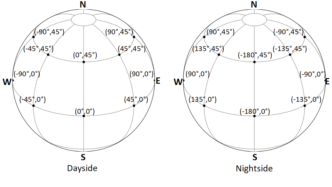
Figure 1: The 3D visualisation of the location of the 16 1D profiles (black dots) that are used to sample the 3D atmosphere for cloud formation, gas-phase chemistry and thermal ionisation on WASP-18b on the day (left) and the nightside (right). The sampled longitudes are $\phi=0^{o},45^{o},90^{o},135^{o},-180^{o},-135^{o},-90^{o}$, the latitudes are at the equator and $\theta=0^{o},45^{o}$ in the northern hemisphere. The 3D simulations assume the southern hemisphere being similar to the northern hemisphere. The substellar point is $(\theta,\phi)=(0^{o},0^{o})$, the terminators are at $\phi=90^{o},-90^{o}$. The sketches indicate East and West which, however, need to be quoted with respect to the day or the nightside.

WASP-18b is an ultra-hot Jupiter, being among the hottest close-in gas giants known so far (Parmentier et al. 2018). Its ultra-short period cause very high irradiation from its F-type star and, hence leads to a extreme temperature difference between day- and nightside (Komacek & Showman 2016). Nymeyer et al. (2011) suggest that WASP-18b has an extremely low Bond albedo and very inefficient day/nightside energy redistribution, a conclusion supported by Iro & Maxted (2013); Schwartz & Cowan (2015). The near Ks-band secondary eclipse observations in combination with the previously obtained Spitzer data suggest that a better thermal mixing is to be expected at higher pressures deeper in the atmospheres (Zhou et al. 2015). Sheppard et al. (2017) find that WASP-18b might have a non-solar C/O $\sim\,1$ based on a radiative transfer retrieval method that includes a selected number of absorbing species (H₂, H₂O, CH₄, NH₃, CO, CO₂, HCN, C₂H₂, CIA of H₂-H₂, H₂-He; Gandhi & Madhusudhan 2018). H₂O, TiO and VO were expected in their dayside emission spectroscopy from HST secondary eclipse observations but were not found. Arcangeli et al. (2018) found that neglecting H^- as opacity source and the thermal dissociation of H₂O would push their retrieval results to high C/O ratios for the evaluation of secondary eclipse observations with HST WFC3 (1.1$\,\ldots\,1.7\mu$m) and combined with Spitzer IRAC (3.5, 5.8 and 8.0 $\mu$m) both providing dayside emission spectra. By including both effects, the metallicity was constrained to approximately solar and an atmospheric C/O¡0.85. Arcangeli et al. (2018) confirm the minimal day-night energy redistribution found by previous authors and the presence of a thermal inversion on the dayside.

This paper begins a consistent analysis of cloud formation and gas-phase chemistry on ultra-hot Jupiters and analysis WASP-18b by applying numerical simulations. We post-process 1D-profiles from a 3D simulation with our kinetic cloud formation model (nucleation, growth/evaporation, gravitational settling, element conservation) that includes a detailed gas-phase calculation and evaluates the thermal ionisation of the gas-phase. We find that WASP-18b forms clouds on the nightside and that thermal ionisation causes the emergence of an ionosphere on the dayside with Mg, Fe, Al, Ca, Na, and K being the most important electron donors in the collisional dominated parts of the atmospheres. Ti⁺ is the most abundant Ti-species on the dayside, not TiO. The enrichment of the atmospheric gas with cloud particles (dust-to-gas ratio, $\rho_{\rm d}/\rho_{\rm gas}$) is rather homogeneously of the order of $\geq 10^{-3}$. The C/O ratio has increased to $>0.7$ in the cloud forming regions of WASP-18b’s atmosphere.

Our approach is outlines in Sect. 2 which includes a summary of the cloud formation model. Section 3 present our results for the global cloud properties of WASP-18b, and Sect. 4 the global day-night changes in gas-phase chemistry on WASP-18b. Section 5 offers a discussion on element replenishment representations and a comparisons of WASP-18b to HD 189733b and HD 209458b. Section 6 concludes the paper.

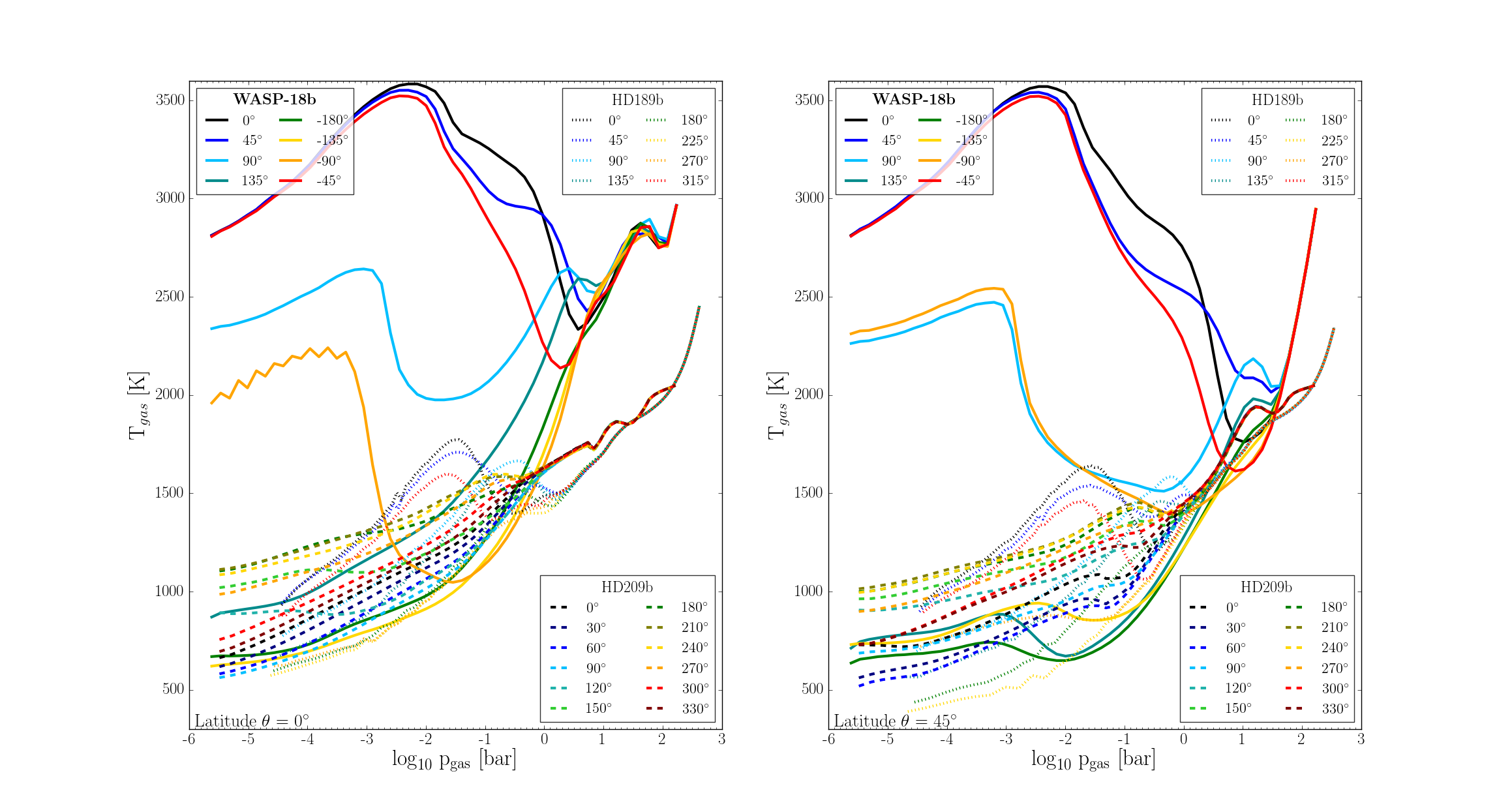
Figure 2: Input gas temperature, T_gas [K], and gas pressure, p_gas [bar], for WASP-18b (Arcangeli et al. 2018), and in comparison to HD 189733b (Dobbs-Dixon & Agol 2013) and HD 209458b (Mayne et al. 2014). WASP-18b is considerably different to HD 189733b and HD 209458b at the days-side but similar temperature regimes occur on the night-side.

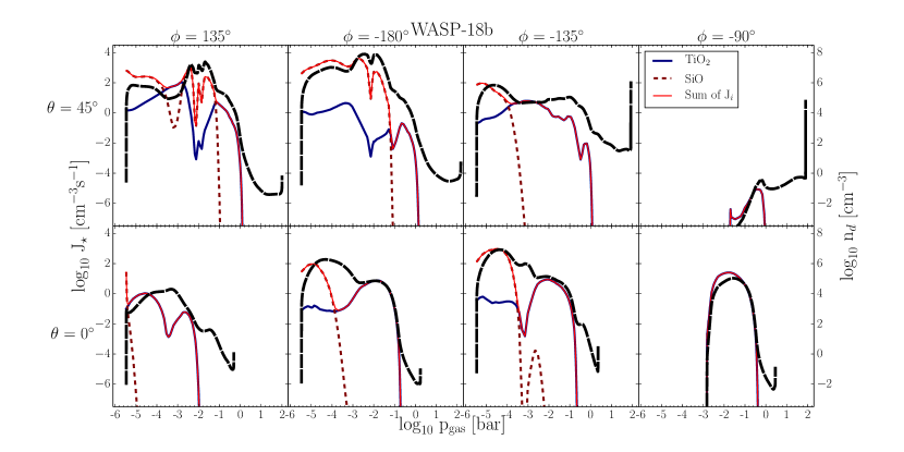
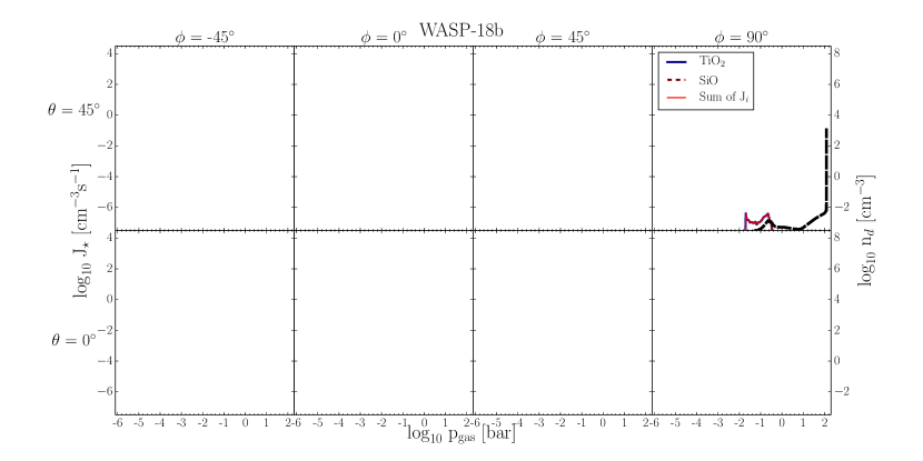
Figure 3: The seed formation rate, J_∗ [cm^-3 s^-1], that triggers the cloud formation (left axis) and the resulting cloud particle number densities, n_d [cm^-3], (right axis, thick dashed line). The total seed formation rate (solid red line) is the sum of the nucleation rate for TiO₂ (solid blue), SiO (dashed brown) and C (dashed gray). Only TiO₂ and SiO form condensation seeds, carbon does not condense in the oxygen-rich environment of WASP-18b. No seed formation occurs on the dayside, hence, no clouds can form, except in the mid-latitudes near the east day/night terminator.

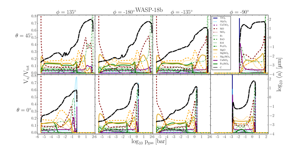
Figure 4: The cloud structure in terms of material composition ($V_{\rm s}/V_{\rm tot}$, $s$ - 15 solid species, left axis, colour coded) and the mean cloud particles size ($\langle a\rangle$ [$\mu$m], right axis, black dashed) on the nightside of WASP-18b. No clouds form on the dayside of WASP-18b. (top: 45^o north, bottom: equator). Some materials reach 100% at the top (SiO[s] (brown dashed), TiO₂[s] (blue solid)) or at the bottom (Fe[s] at $\phi=135^{o},-185^{o}$) of the cloud. Carbon (grey solid) appears with a volume fraction of $\approx 5-10\%$ at some locations.

2 Approach

We apply the two-model approach that we adopted to study the global and the local cloud formation of HD 189733b and HD 209458b in comparison (Helling et al. 2016). We extract 1D (T_gas(z), p_gas(z), v${}_{\rm z}(x,y,z)$)-profiles (T_gas(z) – local gas temperature [K], p_gas(z) – local gas pressure [bar], v_z(x,y,z) – local vertical velocity component [cm s^-1]) from 3D hydrodynamic atmosphere simulations across the globe and use these structures as input for our kinetic, non-equilibrium cloud-formation code Drift (Woitke & Helling 2003, 2004; Helling & Woitke 2006; Helling et al. 2008b). The 3D thermal and wind structure of WASP-18b were calculated using the SPARC/MITgcm (Showman et al. 2009) . We refer to the individual papers regarding more details on the 3D simulations and also the cloud formation modelling (see below). SPARC/MITgcm used here did not implement radiative feedback by clouds. This approach has the limitation of not taking into account the potential effect of horizontal winds on the cloud formation. We note that the cloud formation processes are determined by the local thermodynamic properties which are the result of the 3D dynamic atmosphere simulations. Horizontal winds would affect the cloud formation profoundly if the horizontal wind time-scale would be of the order of the time-scales of the microscopic cloud formation processes. Another aspect is the transport of existing cloud particles through horizontal advection which can not be considered in the approach that we follow in this paper. Horizontal advection as transport mechanisms for cloud particles will play a role if the frictional coupling between gas and cloud particles is sufficient. A frictional decoupling emerges for large enough cloud particles or for low enough gas densities as explored in Woitke & Helling (2003). Horizontal transport will only affect our results if the wind blows in the right direction (night $\rightarrow$ day), and if the advected cloud particles remain thermally stable. Vertical decoupling is included in the approach used here as part of the cloud formation formalism (Sect. 2.1). Woitke & Helling (2003) have further shown that latent heat release is negligible for the condensation of the materials considered if forming from a solar element abundances gas.

2.1 Kinetic formation of cloud particles from oxygen-rich gases

Cloud formation in extrasolar atmospheres requires the formation of seed particles because giant gas planets have no crust like rocky planets. Rocky planets, like Earth, sweep up cloud condensation nuclei (CCNs) through sand storms, volcano outbreaks, wild fires, and ocean spray. Condensation seeds provide a surface onto which other materials can condense more easily as surface reactions are considerably more efficient than the sum of chemical gas phase reactions leading to the formation of the seed. The formation of the first surface out of the gas phase proceeds by a number of subsequent chemical reactions that eventually result in small seed particles. Such a chain of chemical reactions can proceed by adding e.g. a molecular unit during each reaction step (e.g., Jeong et al. 2000; Plane 2013). Goumans & Bromley (2012), for example, show that condensation occurs from small gas-phase constituent like MgO and SiO, which will lead to the formation of bigger units like Mg₂SiO₄ during the condensation process. It is important to realize that big molecules like Mg₂SiO₄ or Ca₄Ti₃O₁₀ do not exist in the gas phase (see Woitke et al. 2017). In this paper, we follow our kinetic cloud formation approach and refer the reader for details on the theoretical background to the references provided below.

Nucleation (seed formation): We apply the concept of homogeneous nucleation to model the formation of TiO₂, SiO and carbon seed particles (Helling & Fomins 2013; Lee et al. 2015b, 2018). We consider the simultaneous formation of these three different nucleation species in contrast to our previous works. In order to do so, we combine our previous works Lee et al. (2015b) (for TiO₂ and SiO) and Helling et al. (2017) (for carbon). The effective nucleation rate, $J_{*}=\sum_{i}J_{\rm i=TiO2,SiO,C}$ [cm^-3 s^-1], determines the number of cloud particles, n_d [cm^-3], and hence, the total cloud surface (as sum of the surface of the cloud particles).

Bulk growth/evaporation: It is essential that the seed forming species are also considered as surface growth material as both process (nucleation and growth) compete for the participating elements (here: Ti, Si, O, C). We consider the formation of 15 bulk materials (TiO₂[s], Mg₂SiO₄[s], MgSiO₃[s], MgO[s], SiO[s], SiO₂[s], Fe[s], FeO[s], FeS[s], Fe₂O₃[s], Fe₂SiO₄[s], Al₂O₃[s], CaTiO₃[s], CaSiO₃[s], C[s]) that form from 9 elements (Mg, Si, Ti, O, Fe, Al, Ca, S, C) by 126 surface reactions (Table 3). We solve moment equations for the cloud particle size distribution function that consider nucleation, growth/evaporation, gravitational settling and mixing (Woitke & Helling 2003; Helling & Woitke 2006; Helling et al. 2008b, c; Helling & Fomins 2013). The growth speed is $\chi$ [cm s^-1] the sign of which is determined by the effective supersaturation ration, $S_{\rm eff}$. If $S_{\rm eff}<1$, $\chi<0$ and the cloud particles evaporate. The approach presented in Woitke & Helling (2003), and utilized in this paper, applies force balance between friction and gravity to derive a size-dependent drift velocity which is required to determine a drift dependent growth term in the moment equations (gravitational settling).

In addition to the local element abundances, $\varepsilon(z)$, also the local thermodynamic properties $T_{\rm gas}(z)$ and $\rho_{\rm gas}(z)$ (local gas density, [g cm^-3]) determine if atmospheric clouds can form, to which sizes, ($\langle a\rangle$ [$\mu$m] – mean cloud particle size), the cloud particles grow and of which materials, s (e.g. TiO₂[s], Mg₂SiO₄[s], MgSiO₃[s], $\ldots$), they will be composed. The gravitational settling velocity ($v_{\rm drift}$ [cm s^-1]) is determined by the local gas density, $\rho_{\rm gas}(z)$, and the cloud particle size.

Element conservation: An additional set of equations for all involved elements is solved with source/sink terms for nucleation, surface growth/evaporation, gravitational settling.

Element replenishment: Cloud particle formation depletes the local gas phase, and gravitational settling causes these elements to be deposited for example in the inner (low pressure) atmosphere where the cloud particles evaporate. For a stationary cloud to form, element replenishment needs to be modelled. We apply the approach outline in Lee et al. (2015a) (Sect. 2.4) using the local vertical velocity to calculate a mixing time scale, $\tau_{\rm mix}\sim v_{\rm z}(r)^{-1}$. We discuss the use of constant vertical diffusion coefficient, $\tau_{\rm mix}\sim K_{\rm zz}^{-1}$ in Sect. 5.1.

2.2 Chemical gas composition

We apply chemical equilibrium (thermochemical equilibrium) to calculate the chemical gas composition (represented in terms of number densities n_x [cm^-3]) of the atmospheres as part of our cloud formation approach. We use the 1D (T${}_{\rm gas}(z)$, p${}_{\rm gas}(z)$) profiles and element abundances $\varepsilon_{\rm i}(z)$ (i=O, Ca, S, Al, Fe, Si, Mg, Ti, C) depleted by the cloud formation processes. All other elements are assumed to be of solar abundance. We use the GGChem routines that recently were made publicly available through Woitke et al. (2017). A combination of $156$ gas-phase molecules, $16$ atoms, and various ionic species were used under the assumption of LTE. The respective material data are benchmarked (Woitke et al. 2017). High velocities and/or strong radiation may cause departure from LTE. Visscher et al. (2006, 2010); Zahnle et al. (2009); Line et al. (2010); Kopparapu et al. (2012); Moses et al. (2011); Venot et al. (2012) have shown that in warm exoplanet atmospheres (T¿1200 K), the chemical timescales are in fact short, and hence thermo-chemical equilibrium prevails in particular in the cloud-forming regions that we are interested.

No condensates are part of our chemical equilibrium calculations in contrast to equilibrium condensation models. The influence of cloud formation on the gas phase composition results from the reduced or enriched element abundances due to cloud formation and the cloud opacity impact on the radiation field, and hence, on the local gas temperature and gas pressure. The element depletion or enrichment due to cloud formation is therefore directly coupled with the gas-phase chemistry calculation.

2.3 Input and boundary conditions

Element abundances: We assume that WASP-18b has an oxygen-rich atmosphere of approximately solar element composition. We use the solar element abundances from Grevesse et al. (2007) (Table 2) as initial values for the cloud formation simulation and outside the cloud forming domains.

Input profiles from a 3D atmosphere simulation for WASP-18b: We use 1D profiles from a 3D atmosphere code which are globally distributed as shown in Fig. 1. The geometry is north-south symmetric. The 3D thermal and wind structures were calculated using the SPARC/MITgcm (Showman et al. 2009). The hydrodynamic model solves the primitive equations on a cube sphere grid. It has been successfully applied to a wide range of hot Jupiters (Showman et al. 2009; Parmentier et al. 2013; Kataria et al. 2015a, 2016; Lewis et al. 2017)including a few ultra hot Jupiters (Zhang & Showman 2018; Kreidberg et al. 2018).

Molecular and atomic abundances in the 3D code are calculated using a modified version of the NASA CEA Gibbs minimization code as part of a grid previously tabulated and used to explore gas and condensate equilibrium chemistry in substellar objects (Moses et al., 2013; Skemer et al., 2016; Kataria et al., 2015a; Wakeford et al., 2017; Burningham et al., 2017; Marley et al., 2017) over a wide range of atmospheric conditions. We consider $\approx 500$ gas-phase species and condensates containing the elements H, He, C, N, O, Ne, Na, Mg, Al, Si, P, S, Cl, Ar, K, Ca, Ti, Cr, Mn, Fe, and Ni. We assume solar elemental abundances and local chemical equilibrium with rainout of condensate material taken into account, but no interaction between the gas phase and the solid phase.

The opacities of major molecules (CO, H₂O, CH₄, NH₃, TiO, VO, CrH, FeH, CO₂, PH₃, H₂S), alkali atoms (Na, K, Cs, Rb, and Li), and continuum (collision induced absorption due to H2-H2, H2-He and H2-H, bound-free absorption by H and H- and free-free absorption are taken into account following Freedman et al. (2008) and Freedman et al. (2014). The radiative transfer is performed within 8 k-coefficients inside each of the 11 wavelengths bins (Kataria et al., 2015b). We used a timestep of 25s, ran the simulations for 300 days and averaged all quantities over the last 100 days. The above modelling process is the same as that described in Parmentier et al. (2016), using the WASP-18 system parameters from Southworth et al. (2009)

The model, as all global circulation models studying these hot planets suffers from some important limitations. The model does not include magnetic interactions between the planetary magnetic field and the ionised gas (Rogers & Showman, 2014; Rogers, 2017), latent heat transport through the recombination of $\rm H_{2}$ (e.g. Bell & Cowan, 2018) nor cloud opacities (Parmentier et al., 2016; Roman & Rauscher, 2017). We therefore expect that large scale structure such as the day/night contrast or the east/west terminator difference to be accurate within an order of magnitude, but exact temperatures and winds speeds might change  (Koll & Komacek, 2018, e.g.).

WASP-18b’s planetary parameter: We use $T_{\rm equ}=2411$K (Sheppard et al. 2017), assume a constant value $g=19043$ cm $s^{-2}$ ($R_{\rm P}=8.328818\cdot 10^{9}$ cm, $M_{\rm P}=1.979614\cdot 10^{31}$g, Hellier et al. 2009) and a constant mean molecular weight for a H₂ dominated gas ($\rm\mu$ = 2.3 m_μ). The local gas density $\rho_{\rm gas}(z)$ is calculated from the given gas pressure by applying the ideal gas law, $\rho_{\rm gas}(z)=P_{\rm gas}(z)\mu m_{\mu}/(k_{B}T_{\rm gas}(z))$. In order to find the height of each of the atmospheric layer inside the 53 vertical computational domains, hydrostatic equilibrium is assumed in vertical direction. The hydrostatic equilibrium equation is integrated to convert the given pressure into a height coordinate. The inner integration boundaries are the planet radius where $p_{\rm gas}=1$ bar.

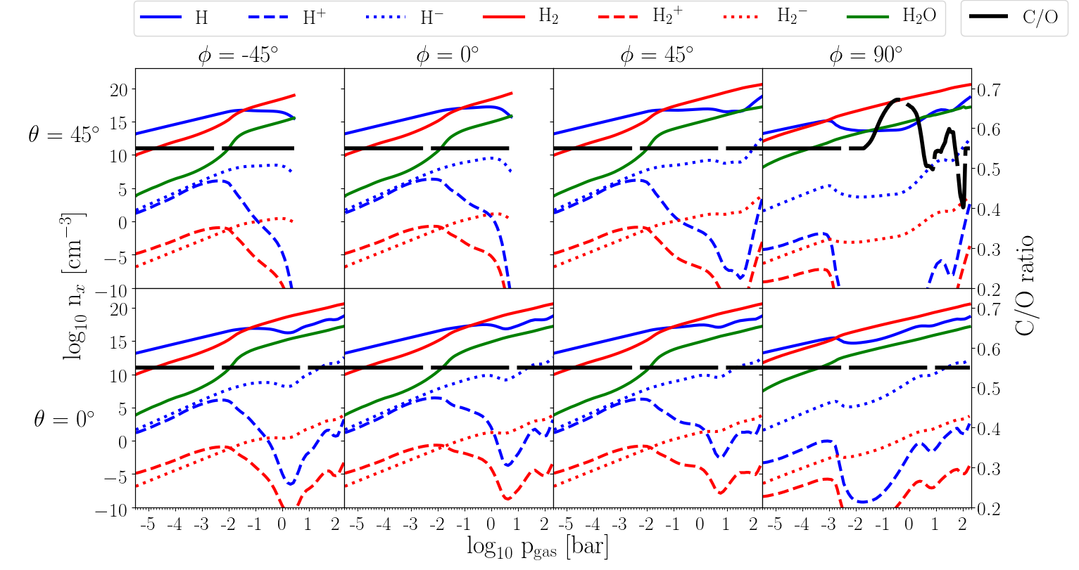
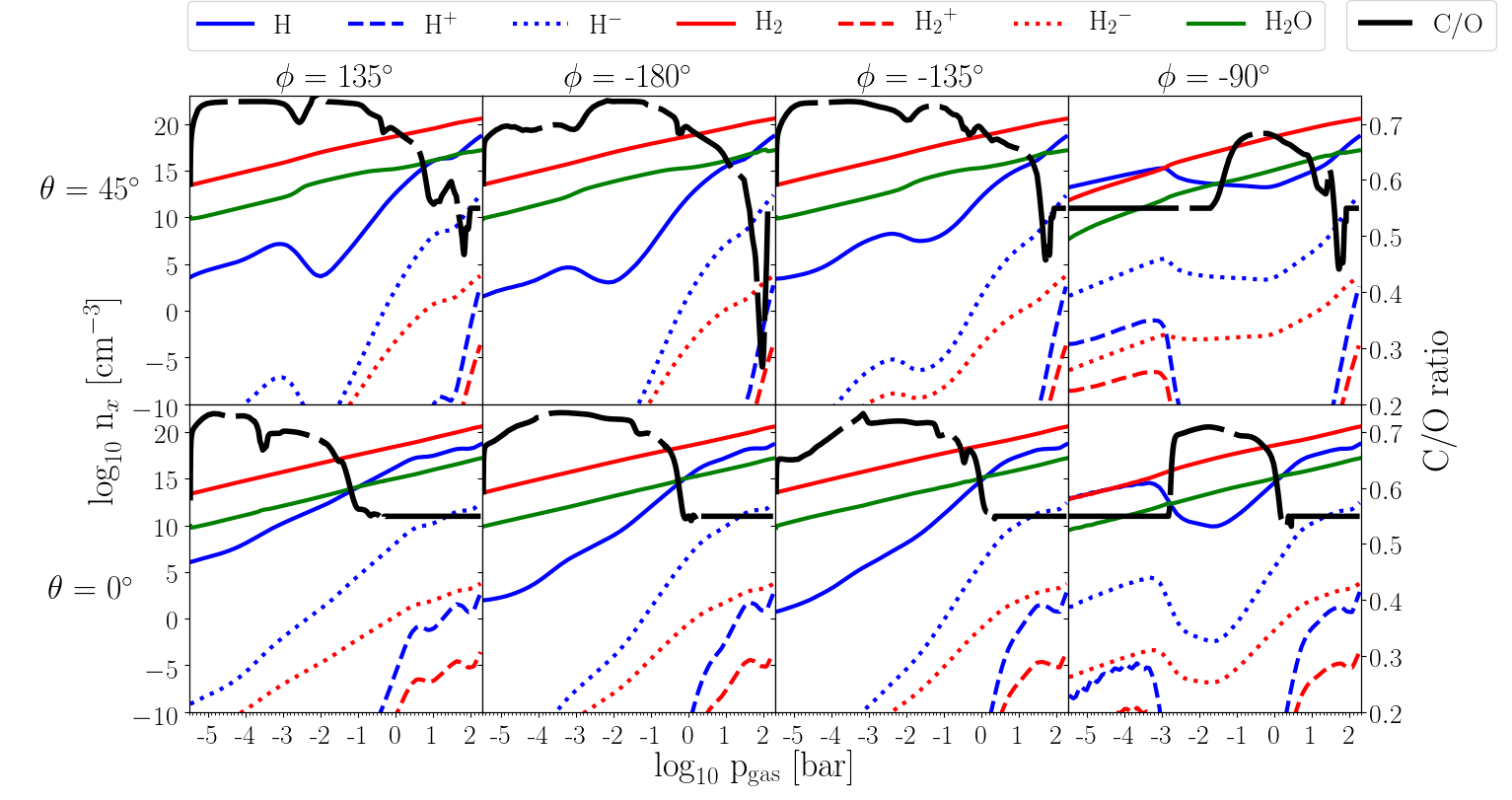
Figure 13: Number densities, log $n_{\rm x}$ [cm^-3], of H-binding gas-species (color coded, left axis). The C/O is overplotted and shows where cloud affects the atmosphere (black long-dashed line, right axis).

We introduce a small uncertainty by using $\rm\mu$ = 2.3 m_μ if H₂ would dissociate. We show in Fig. 13 that thermal H₂ dissociation only occurs on the dayside of WASP-18b where no clouds can form. Hence, this assumption does not affect our cloud formation results for which the above procedure is required in order to derive the geometric extension of the numerical grid.

3 The global cloud properties of WASP-18b

We study if and which kind of clouds could form on WASP-18b by sampling 8 different profiles at the equator and 8 in the mid-latitude region. We endeavour to provide a first insight into the global and the local cloud structure for a planet that is expected to show vastly different day and nightsides.

Figures 2 summarise the input profiles that we use to study cloud formation at the day- (longitude $\phi=0^{o}$, $45^{o}$, $-45^{o}$) and the nightside (longitude $\phi=-180^{o}$, $135^{o}$, $-135^{o}$) of WASP-18b as well as at the day/nightside terminators (longitude $\phi=90^{o}$ and $\phi-90^{o}$). The differences in the thermodynamic structures are very large: Day and nightside temperature have a difference of upto 2500K. The dayside profiles can be as hot as 3500K at a relatively low pressure of p${}_{\rm gas}=10^{-3}$ bar. The terminator regions show strong temperature inversions causing a steep local (inward) drop in temperature of up to 1000K. Such thermodynamic differences suggest that cloud and gas-phase chemistry will differ strongly between the day and the nightside of the planet. This temperature inversion may cause the appearance of emission features due the emergence of an outward increasing temperature gradient.

WASP-18b in comparison to HD 189733b and HD 209458b: In reference to our previous studies (Helling et al. 2016), Fig. 2 shows the WASP-18b 1D profiles in comparison to the 1D profiles from HD 189733b and HD 209458b. Both, HD 189733b and HD 209458b have atmospheres that are filled with clouds on the day and the nightside, though their detailed characteristics (like cloud particle size, material composition) differ. WASP-18b has a much hotter inner atmosphere compared to HD 189733b and HD 209458b at the equator and in the hemispheres, but reaches comparable low temperatures at the nightside. The dayside is hotter by about 2500K compared to HD 189733b and HD 209458b in the equator region. The day/nightside temperature difference for HD 189733b and HD 209458b are $\approx 500K$ compared to the 2000K on WASP-18b at local gas pressure of $10^{-5}\,...\,10^{-2}$bar (see Fig. 2).

Our first result is that no clouds form on the dayside (Fig. 3), hence, a non-depleted warm gas-phase chemistry should be observed. However, a depletion of the gas-phase could occur if cloud particles can be transported horizontally from the nightside to the dayside and if, at the same time, the local supersaturation is large enough to allow for surface growth processes. A depletion of the dayside gas-phase could also occur if the depleted gas from the nightside is advected on the dayside faster than the vertical mixing occurs (see Parmentier et al. 2013). In-situ cloud formation only takes place in the day/nightside terminator regions and on the nightside equator and in the hemispheric regions on WASP-18b. The northern dayside terminator profile ($\theta=45^{o}$, $\phi=90^{o}$) does form seed particles, but the equator dayside terminator profile ($\theta=0^{o}$, $\phi=90^{o}$) remains cloud-free as superrotation affects the equatorial temperature such that the mid-latitudes are colder than the equator (compare also Fig. 2). The supersaturation of the gas is very low ($<10^{-5}$) at the $(\theta,\phi)=(0^{o},90^{o})$ terminator (see Fig. 5). Cloud formation on the dayside remains therefore very unlikely even if condensations seeds would be swept along with the winds given that the temperatures on the dayside are even higher. On the nightside, a vast amount of cloud particles form leading to a dust-to-gas-ratio of $\geq 10^{-3}$ and an increase in the atmospheric C/O to $>0.7$. Arcangeli et al. (2018) derive a disk-averaged C/O $<0.85$ from their emission spectre, hence for the day-side of WASP-18b. We predict that the dayside C/O ratio should be unaffected by cloud formation. If this primordial C/O were close to the upper bound of 0.85, then cloud formation could drive the C/O on the nightside to values large enough to change significantly the atmospheric chemistry and lead to an observable signature (Helling et al. 2014). Molecules like HCN and CN might be detectable. The increase of C/O to $>0.7$ (starting from solar values) does only occur on the nightside in our simulation.

3.1 The nightside of WASP-18b

Figure 3 demonstrawhere in the atmosphere WASP-18b cloud formation is triggered through the nucleation of condensation seeds. We consider the simultaneous formation of TiO₂ (solid blue), SiO (brown dashed) and C (solid gray) seed particles (left axis). The sum of these seeds then provides the total number of cloud particles (long dashed black lines, right axis) locally. The comparison between the total nucleation rate, $J_{*}$ [cm^-3s^-1], the cloud particle number density, $n_{\rm d}$ [cm^-3] and Fig. 4 reveals that the vertical cloud extension encompasses a larger volume (plotted in terms of pressure) than the nucleation regions would suggest. This difference demonstrates that cloud particles are transported vertically through gravitational settling into the deeper atmosphere.

Figure 3 further demonstrates that SiO and TiO₂ do efficiently nucleate in the uppermost atmospheric regions until $\approx$ 2200K in the model structures used here. Carbon does not nucleate for all probed profiles. TiO₂ remains efficient also at higher temperatures due to the combined effect of element consumption by material growth and temperature. TiO₂ is the sole nucleation species for the hotter nightside east-terminator ($\phi=-90^{o}$) at the equator and in the mid-latitudes.

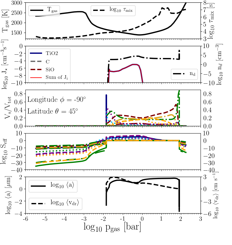
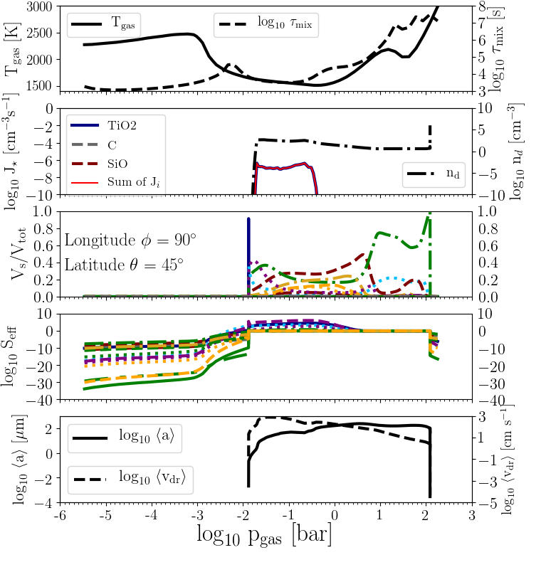
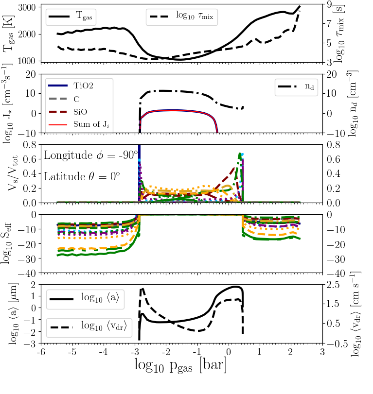
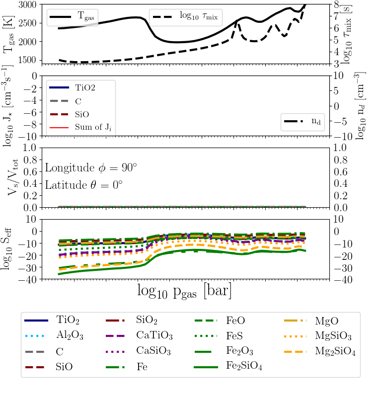
Figure 5: The combined view on the cloud structure of the profiles probing each of day-night-terminators of WASP-18b (top: 45^o north, bottom: equator; left: west, right: east seen from the dayside). Following earlier works (e.g. Fig. 9 in Helling & Casewell 2014), we summarise the fundamental cloud properties for each of the limb profiles to demonstrate the differences in cloud details and their causes. For each profile the plots show the following properties as function of the local gas pressure p_gas [bar] : 1st panel: local gas temperature, T_gas [K] (solid, left), mixing time scale $\tau_{\rm mix}$ [s] (dashed, right). 2nd panel: total nucleation rate, J_∗ [cm^-3 s^-1] (red), and the individual rates for TiO₂ (blue), SiO (brown dashed), carbon (green dashed); number density of cloud particle, n_d [cm^-3]. 3rd panel: effective growth velocity, $\chi$ [10^-7 cm s^-1]. 4th panel: material volume fraction, $V_{\rm s}/V_{\rm tot}$ with $V_{\rm s}$ the volume of the material s, $V_{\rm tot}$ the volume of all cloud particles. 5th panel: effective supersaturation ratio, $S_{\rm eff}$, per material. 6th panel: mean cloud particle size, $\langle a\rangle$ [$\mu$m] (solid, left), drift velocity $v_{\rm drift}$ [cm s^-1]. The materials are line and colour coded as follows: TiO₂[s] - solid, dark blue; Al₂O₃[s] - dotted, light blue; C[s] - dashed, green; SiO[s] - dashed, brown; SiO₂[s] - dash-dot, crown; CaTiO₃[s] - dashed, purple; CaSiO₃[s] - dotted, purple; Fe[s] - dash-dot, green; FeO[s] - dahsed, green; FeS[s] - dotted, green; Fe₂O₃[s] long-dash-dot, green; Fe₂SiO₃[s] - solid, green; MgO[s] - dash-dot, dark organg; MgSiO₃[s] - dotted, organg; Mg₂SiO₄[s] - dashed, organg. Superrotation prohibits cloud formation on the east equatorial terminator ($\phi=90^{o}$, $\theta=0^{o}$; lower left panels).

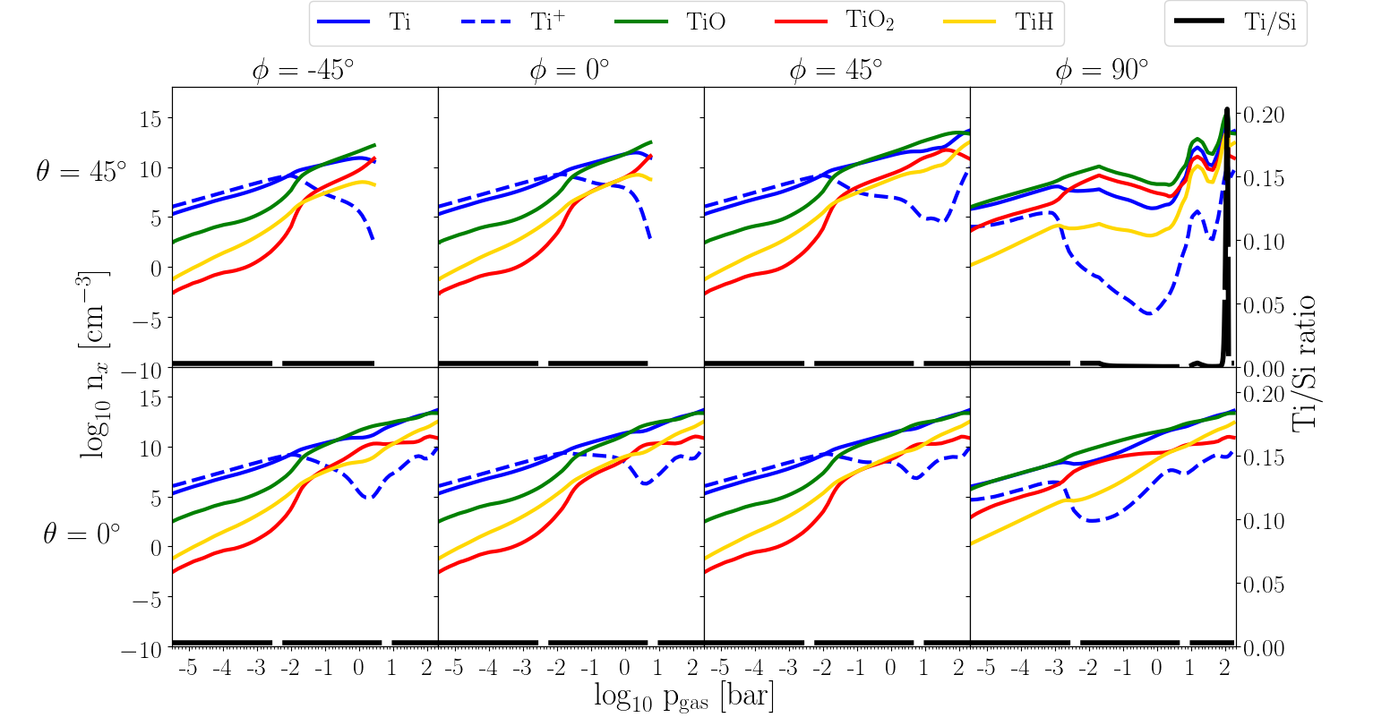
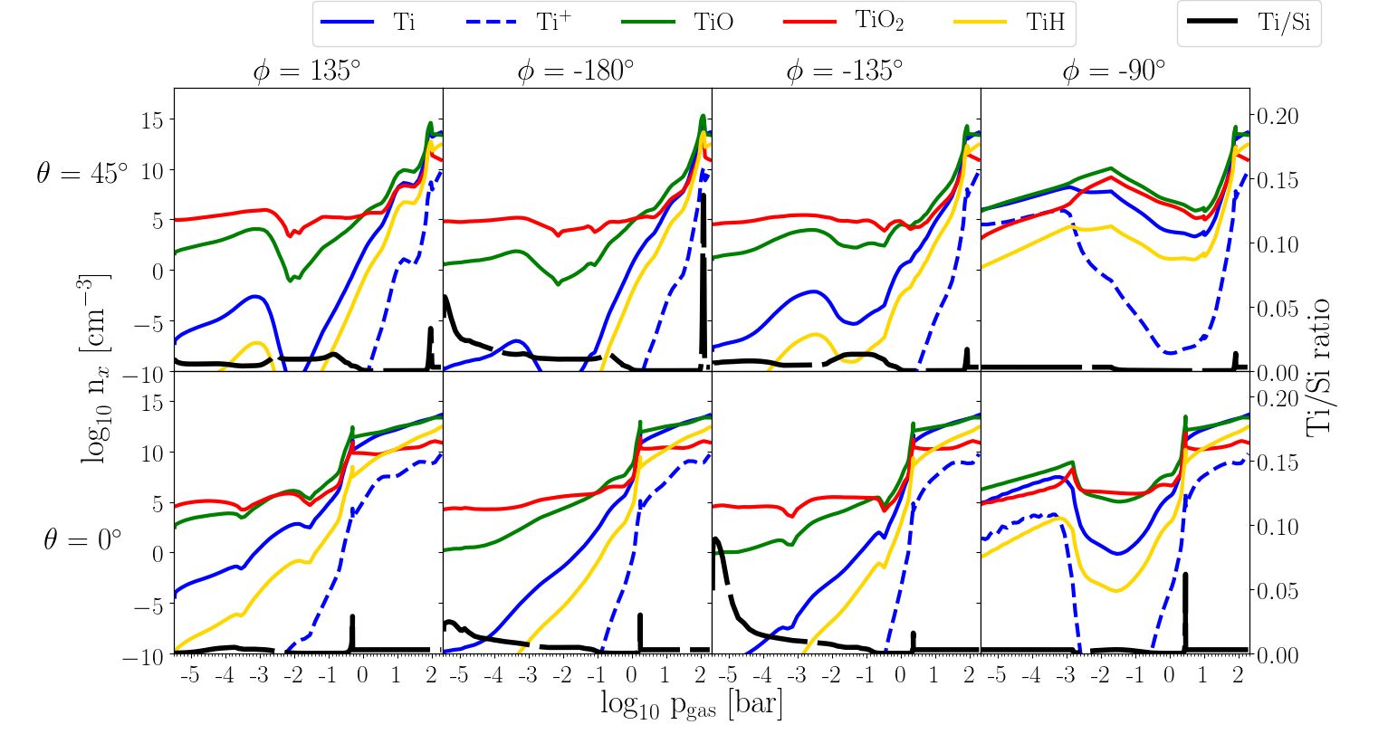
Figure 24: Number densities, log $n_{\rm x}$ [cm^-3], of Ti-binding gas-species (color coded, left axis). The Ca/Si ratio is overplotted and shows where cloud affects the atmosphere (black long-dashed line, right axis).

The dayside of WASP-18b does have no seed formation except at the dayside west terminator ($\phi=90^{o}$). This is a clear indication for that WASP-18b will not form any clouds in situ at its dayside because the local temperatures are simply too high. This conclusion is further emphasized by our study of the gas-phase composition in Sect. 4 and Fig. 24 which shows that Ti⁺ is the dominating Ti-carrier at the days-side of WASP-18b, and not TiO₂ as is the case for most of the nightside. Small cloud particles can move along with the flow and could therefore be transported form the night to the dayside. They could, hence, serve as condensation seeds in the absence of in-situ seed formation. Our investigation of the local gas-phase, however, shows that the dayside of WASP-18b will be too hot to allow for a sufficient supersaturation of the gas phase for condensation to occur.

Figure 4 present the vertical cloud extension, their detailed material composition in units of relative volumes ($V_{\rm s}/V_{\rm tot}$, $s$ - solid species; colour codes lines on left axis) and the vertical distribution of the mean cloud particles ($\langle a\rangle$ [$\mu$m], black solid line on right axis) for the equator (bottom row) and the 45^o-latitude on the northern hemisphere. These 1D cloud maps visualize that the clouds extend over a larger pressure range in the (norther) hemisphere than at the equator region. At the (northern) hemisphere nightside profiles ($\phi=135^{o},-180^{o},-135^{o}$), the entire computational domain is filled with cloud particles. The cloud extension becomes more confined the more westward ($\phi=-135^{o}\longrightarrow-180^{o}\longrightarrow 135^{o}$) we probe the atmosphere on the nightside in the equatorial regions. This confinement does not occur in the northern/southern hemisphere. The mean cloud particles sizes follow the profile of the atmospheric gas that generally has an outward decreasing gas density: The cloud particles size increases inwards and reaches it’s maximum in the densest regions just before it decreases and drops to zero because the local temperature becomes to hot and the cloud particles evaporate. It is interesting to note that the hemispheric ($\theta=45^{o},-45^{o}$) day-night terminator at $\phi=-90^{o}$ forms the largest cloud particles as result of a considerably lower nucleation rate.

The material composition of the cloud particles changes as the local thermodynamic conditions change. The top-most layer is determined by the seed particle forming materials and MgO[s] for all but the $\phi=-135^{o}$-equator profile. As soon as Mg-Si-O and Fe-Si-O materials become thermally stable, a combinations of them makes up the matrix (the bulk) of the cloud particles. Mg₂SiO₄[s], MgSiO₃[s], MgO[s],Fe₂SiO₄[s] make up 60% of the volume with Mg₂SiO₄[s] and MgSiO₃[s] contributing most. This is followed by 20-30% made of SiO[s], SiO₂[s], and FeS[s]. All other materials remain below the 10% level providing a colorful mix of minerals in the Mg₂SiO₄[s]/MgSiO₃[s]-dominated part of the cloud. We note that the cloud particles change in sizes from $\langle a\rangle\approx 10^{-3}\,\ldots\,1\mu$m in this cloud region. The temperature increases when going deeper into the atmospheres at the nightside which causes the Mg-Si-O/Fe-Si-O materials to become thermally unstable and, hence, to evaporate. This results in a substantial material peak of SiO[s] before it evaporates and the high-temperature condensates determine the material composition of the cloud at its hottest rim at low altitudes. The SiO[s] dominates substantially in the warmer regions. 75% of the cloud volume in this layer made of $\approx 1\,\ldots\,2\mu$m-sized particles is made of SiO[s] with MgO[s] ($\approx 20$%) and Fe[s] ($\approx 15$%) with inclusions from CaSiO₃[s] and Al₂O₃[s]. The equatorial region has again the smaller particles also in this cloud region. Once SiO[s] has evaporated, a thin cloud layer made of Fe[s] with CaSiO₃[s] and Al₂O₃[s] inclusions follows. At the equator, one to two additional cloud regions made of almost pure Al₂O₃[s] and below that CaTiO₃[s] form. Al₂O₃[s] and CaTiO₃[s] are the most stable materials in our setup. In the mid-latitudes, the largest cloud particles reach sizes of 100$\mu$m and are made of Fe[s] with CaSiO₃[s] and Al₂O₃[s] inclusions. In the equator region, the largest particles reach 10$\mu$m and are made of - possibly sparkling - Al₂O₃[s] and CaTiO₃[s]. If the cloud particle undergo a heating or are exposed to large pressures, amorphous materials can turn into their crystalline counterparts (e.g. Helling & Rietmeijer 2009) possibly causing clouds to sparkle.

The implication of the cloud formation on the gas-phase chemistry will be discussed in detail in Sect. 4.

3.2 The day/nightside terminator clouds on WASP-18b

WASP-18b is interesting with respect to cloud and gas-chemistry as its thermodynamic set-up varies greatly over the globe (Sect. 2.3). The change-over between ’no clouds’ and ’plenty of clouds’ occurs at the day/nightside terminators which we discuss here separately. Both terminator-regions at the equator and in the northern hemisphere show strong temperature inversions causing an extended, local minimum of the temperature inside the atmosphere.

Figure 5 summarized the cloud details for the four 1D terminator profiles investigated in this paper (top: 45^o north, bottom: equator; left: west, right: east seen from the dayside). The top panel of this figures also show the input properties (T_gas, $p_{\rm gas}$) (solid line, left axis) and the mixing time scale, $\tau_{\rm mix}$ (dashed line, right axis). Cloud formation takes place at three out of the four terminators. The east (seen from the dayside) terminator ($\phi=90^{o}$) at the equator is too hot for clouds to form. But winds will not transport cloud particles from the night side here because the wind moves from the day into the nightside at $\phi=90^{o}$. The terminator exposed to the wind from the nightside ($\phi=-90^{o}$) is cold enough for in situ cloud formation.

The vertical cloud extension varies between the equatorial ($p_{\rm gas}\approx 10^{-3}\,...\,10^{0.5}$ bar) and the norther/southern hemisphere ($p_{\rm gas}\approx 10^{-2}\,...\,10^{2}$ bar) terminator as result of the local temperature. This will have implications for transit spectroscopy. The mean cloud particle sizes vary widely at the equator and less in the norther/southern hemisphere terminator. Differences emerge also for the material compositions. The northern/southern hemisphere terminators (east & west) have cloud particles mainly composed of SiO[s], Fe[s], MgO[s] being less dominated by Mg₂SiO₄[s]/MgSiO₃[s] with inclusions from other materials. The top and the bottom parts of the terminator clouds are dominated by high-temperature condensates: The top is made of thin layers of pure TiO₂[s], followed by a thin layer of a Al₂O₂[s]/CaTiO₃[s] mix, and then a thin Fe[s]/CaTiO₃[s]-dominated layer with inclusions from Al₂O₂[s], SiO[s] and others to a lesser extend. The bottom layer is made of big Fe[s]-dominated particles with some Al₂O₂[s]. The $\phi=90^{o}$ terminator region has a substantial Fe[s]-dominated low-altitude layer in contrast to the $\phi=-90^{o}$ terminator that has a rather thin Fe[s]-dominated inner layer at low-altitudes. The whole low-altitude portion for $p<1$bar is made of big particles of $\approx 32\mu$m which are decelerated by the inward increasing gas density (dashed line, right axis).

The equatorial terminator that forms clouds on WASP-18b is in the west terminator seen from the dayside ($\phi=-90^{o}$). Its cloud top is made of subsequent thin layers of TiO₂[s], Al₂O₂[s], CaTiO₃[s] and Fe[s]-dominated and become more and more a mix of many materials. The major vertical portion of the cloud is made of Mg₂SiO₄[s]/MgSiO₃[s]/MgO[s]/SiO[s]/Fe[s] with inclusions from the other materials. The bottom of the cloud changes from SiO[s] dominated, to Fe[s], then Al₂O₂[s], and then CaTiO₃[s] dominated. These cloud bottom layers are composed of the biggest particles of $\approx 60\mu$m falling with a fall speed of 1.5 cm s^-1 (dashed line, right axis).

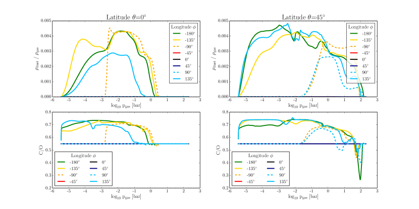
Figure 6: The cloud particle load in terms of mass density ratios (top; $\rho_{\rm dust}/\rho_{\rm gas}$) and the C/O element ratio (bottom) at the equator (left) and in the norther hemisphere (right) of the WASP-18b atmosphere profiles studied. C/O remains at the solar value of 0.53 for profiles without clouds forming ($\phi=-45^{o},135^{o}$). For other mineral rations like Fe/Si, Mg/Si etc., please refer to Appendix A (Figs. 14 – 24).

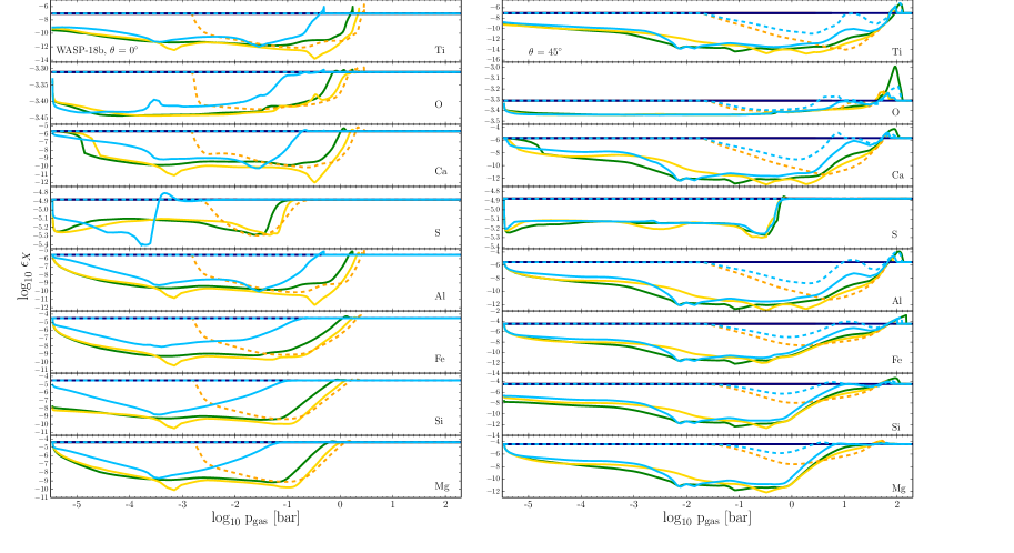
Figure 7: The abundances, $\epsilon_{\rm x}$, of those element involved in cloud formation for the equatorial (left, $\theta=0^{o}$) and the northern hemisphere (right, $\theta=45^{o}$) profiles of WASP-18b. The colour code for the atmospheric profiles is that same as in Fig. 6 and all figures throughout the paper. The day-night terminators are depicted as dashed lines. Straight lines indicate no element depletion for these longitudes. Cloud formation mostly causes element depletion. Element enrichment occurs where cloud particles evaporate, most noticeable for $\epsilon_{\rm O}$. The element abundances change due to cloud formation throughout the atmosphere and across the globe. The clouds affect the element abundances over a larger pressure range at the norther (southern) hemisphere compared to the equatorial region.

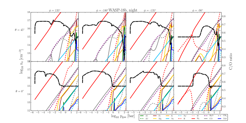
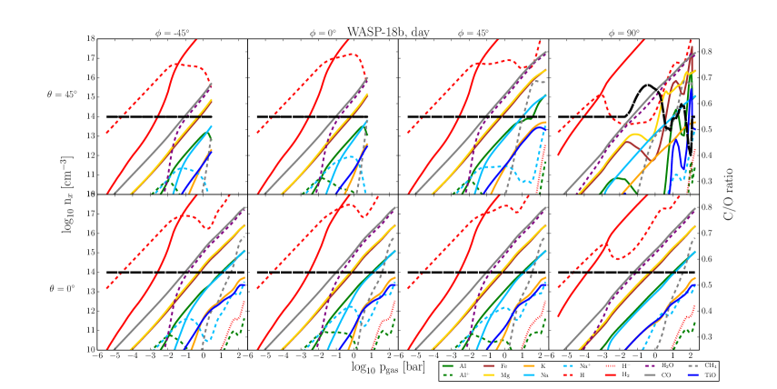
Figure 8: Composition of the atmospheric gas in chemical equilibrium with respect to the most abundant molecules, atoms and ions (number density n_x [cm^-3]) from the night (top) to the dayside (bottom) on WASP-18b. The day- and the nightside have very different chemical atmosphere gas composition. The dayside is dominated by atomic H, the nightside by H₂. The next most abundant gas species are CO, H or H₂ depending ($\theta,\phi$). C/O is over plotted to visualise where clouds form. C/O remains at its initial (solar) value on the dayside where no clouds are forming, but increases on the nightside. A complete account of all species per element is provided in Appendix A.

3.3 Cloud particle load of the atmosphere of WASP-18b

An interesting measure regarding the cloud particle load of the atmosphere is the so-called dust-to-gas mass ratio, $\rho_{\rm dust}/\rho_{\rm gas}$ (Fig. 6, top). This measure for the enrichment of a gaseous medium with condensates (often solid) is widely used in disk modelling where it is set to a constant value (e.g. Alessi & Pudritz 2018), or to study the dust enrichment of cometary tails (e.g. Fulle et al. 2010; Langland-Shula & Smith 2011) or AGB star envelopes (e.g. Helling et al. 2000; Ramstedt et al. 2011). Woitke et al. (2017) have demonstrated that the dust-to-gas mass ratio changes with temperature for a system in thermal equilibrium (i.e. everything that can condense has condensed). The main contributors are materials involving Al, Ca, Fe, Si and Mg. Condensates composed of titanium, nickel, vanadium, chromium, manganese, sodium and potassium contribute only very little as their initial element abundances are very low. The maximum value reached in thermal equilibrium is $\rho_{\rm dust}/\rho_{\rm gas}\approx 0.004\,\ldots\,0.0052$ for gases $>500$K and (Fig. 5 in Woitke et al. 2017).

The cloud particle load of the atmospheric gas in WASP-18b varies vertically with the maximum of $\rho_{\rm dust}/\rho_{\rm gas}\approx 0.0042$ being reached at $p\approx 10^{-2}$bar in the equatorial region and $\rho_{\rm dust}/\rho_{\rm gas}\approx 0.0049$ at lower pressure of $p\approx 10^{-3}$bar in the mid-latitudes on the nightside. $\rho_{\rm dust}/\rho_{\rm gas}$ clearly shows that the cloud layers are located much farther inside the atmosphere and are considerably less extended at the day-night-terminators. This indicates the transitional character of the planet’s limbs where a hot dayside transits into a cold nightside. No one $\rho_{\rm dust}/\rho_{\rm gas}$ can describe the profiles studied here. However, the $\rho_{\rm dust}/\rho_{\rm gas}$ is of the order of $10^{-3}$ for all probed profiles suggesting a globally rather homogeneous cloud particle load in regions where clouds form.

4 The global changes of the atmospheric gas composition on WASP-18b

The large temperature (and pressure) difference between the day- and the nightside on WASP-18b and the transitional character of the terminator regions lead to a distinct cloud distribution on WASP-18b. We therefore expect the atmospheric gas composition on WASP-18b to be vastly different on the day- and the nightside, too. We have considered 15 materials which affect the element abundances of the 9 (Mg, Si, Ti, O, Fe, Al, Ca, S, C) elements by cloud particle growth and evaporation by 126 surface reactions. The growth process reduces the element abundances, the evaporation process enriches the element abundances. The nucleation process has only very little affect on the element involved (Si, Ti, O, C), but it is strongly affected by element depletion.

4.1 Element depletion and enrichment

One of the most important outcomes of a cloud formation model is the feedback on the gas phase through element depletion or enrichment. The essential quantities to start with are the element abundances as the number of elements needs to be conserved for each element individually. Figures 7 demonstrates the consistency of our cloud formation model because cloud formation only affects the involved elements at the nightside and at the day/night-terminators.

Each of the elements is individually depleted and the depletion varies widely through the cloud structure (along the pressure axis) and across the globe. The largest variations in element depletion for any one element occurs along the equator for WASP-18b (Fig. 7, left plots). The day/nightside terminators stand out by depleting a less extended atmosphere of the vertical atmosphere at the equator and in the hemispheres.

A closer look at Fig. 7 shows that the individual depletion of the elements varies by order of magnitudes. Ti is strongest depleted but it also has the smallest initial element abundance of all involved cloud forming elements. Some elements show a substantial enrichment at the inner cloud boundary located at low-altitudes due to the evaporation of cloud particles that have been falling until such high temperatures. Most noticeable is the effect in the mid-latitudes (right of Fig. 7) for Ti, O, Ca, Al and Fe. Si is enriched, too, compared to the initial solar values but far less than the other elements. Therefore, element enrichment occurs in deep, unobservable layers of the atmosphere. Observable layers are expected to be depleted in all elements that are involved in cloud formation.

Oxygen is one of the most abundant elements in a solar set of element abundances and it is involved in almost every growth material that easily forms. We therefore portrait the oxygen-depletion also as C/O ratio in Fig. 6.

4.2 C/O and [X/Si] element ratio

The most prominent element ratio studied in the literature is the carbon-to-oxygen ratio, C/O. C/O is of interest with respect to planet formation scenarios and the link to the chemistry in planet forming disk (e.g. Helling et al. 2014; Eistrup et al. 2018). C/O, Mg/Si and Fe/Si are discussed in the literature as control parameter for the amount of carbides and silicates formed in planets (Adibekyan et al. 2017; Suárez-Andrés et al. 2018). Our results show that the thermodynamic properties of the local gas determine the condensation processes from which element ratios like C/O (Fig. 6) and X/Si (Figs. 14 – 24) result.

The largest change in the C/O throughout the cloud-affected part of the atmosphere occurs in the northern/southern hemisphere. Here the larges and the smallest C/O is reached. C/O is bound between 0.28 and 0.73. Only a C/O ration above 0.93 will allow first carbon-binding molecules to emerge (TiC; Woitke et al. 2017). Bedell et al. (2018) show that C/O varies between 0.4 and 0.6 for the solar twins in the solar neighborhood. No one atmospheric C/O will suffice to describe the atmosphere of WASP-18b. First, it varies vertically throughout the atmosphere and it varies globally. C/O remains solar at the dayside where no clouds form and becomes enriched/depleted on the cloud-forming nightside. The C/O at the night side shows the change from a thermally stable to a thermally unstable cloud. C/O increases above the initial (solar) value of 0.53 in the thermally stable part of the atmosphere but decreases substantially where the cloud particles evaporate. The increase in C/O is mainly caused by oxygen consumption and the decrease in C/O is mainly caused by oxygen being transported into deeper atmospheric regions due to falling cloud particles. The width of the O-enriched zone shows that the cloud particles do not evaporate instantaneously. If carbon-materials form, carbon depletion/enrichment will affect the C/O ratio, too. Our calculations show the condensation of only very little carbon on the nightside of WASP-18b (5-10%; Fig 4).

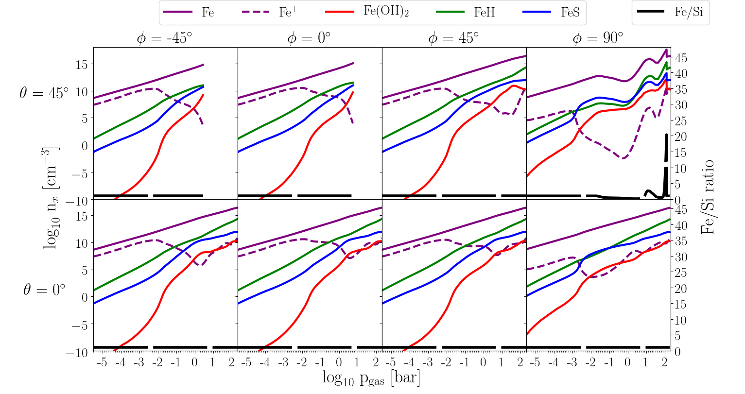
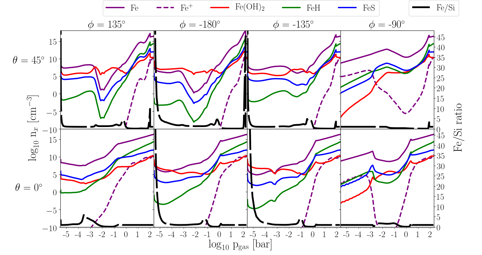
Figure 18: Number densities, log $n_{\rm x}$ [cm^-3], of Fe-binding gas-species (color coded, left axis). The Fe/Si ratio is overplotted and shows where cloud affects the atmosphere (black long-dashed line, right axis).

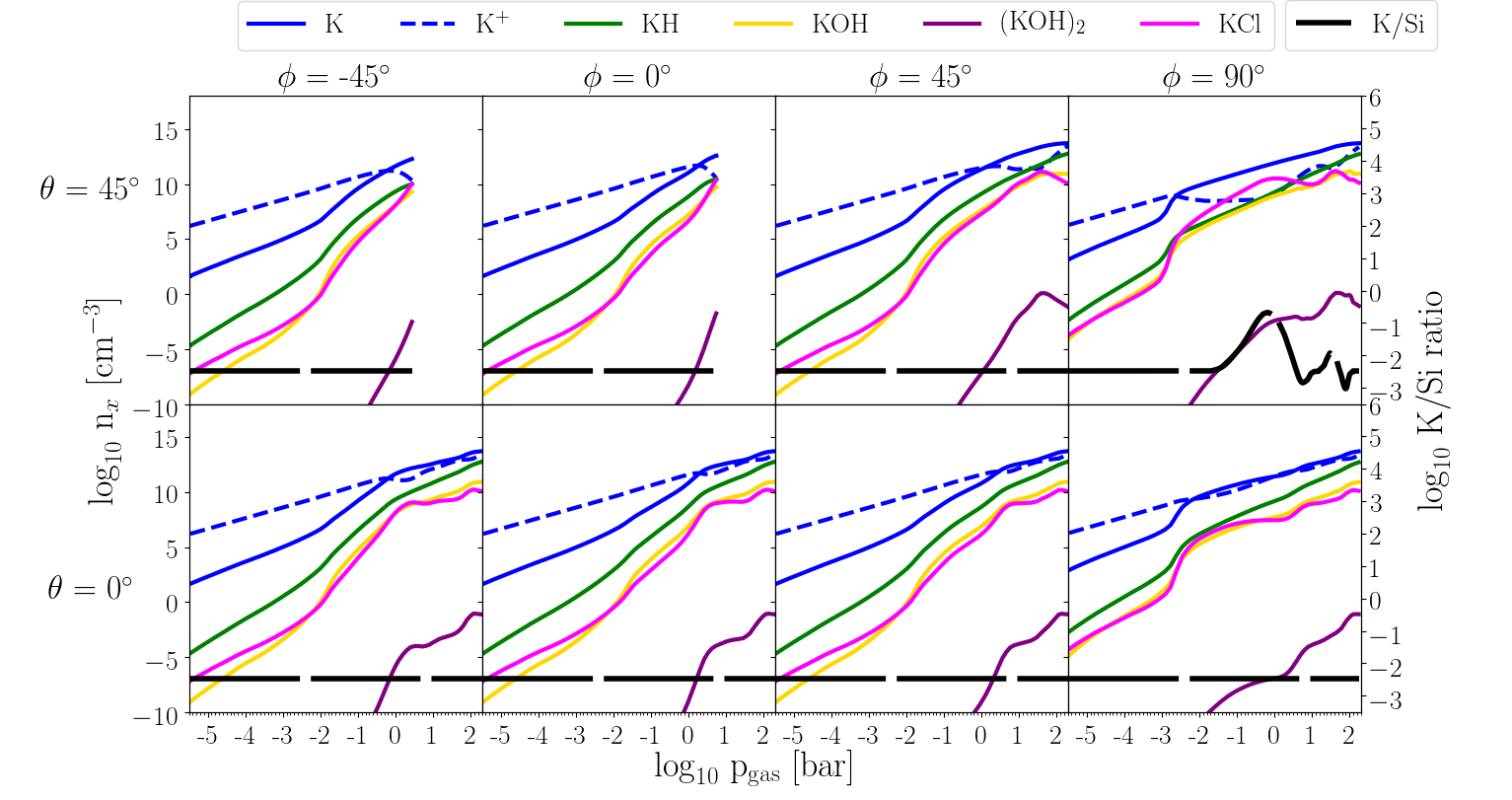
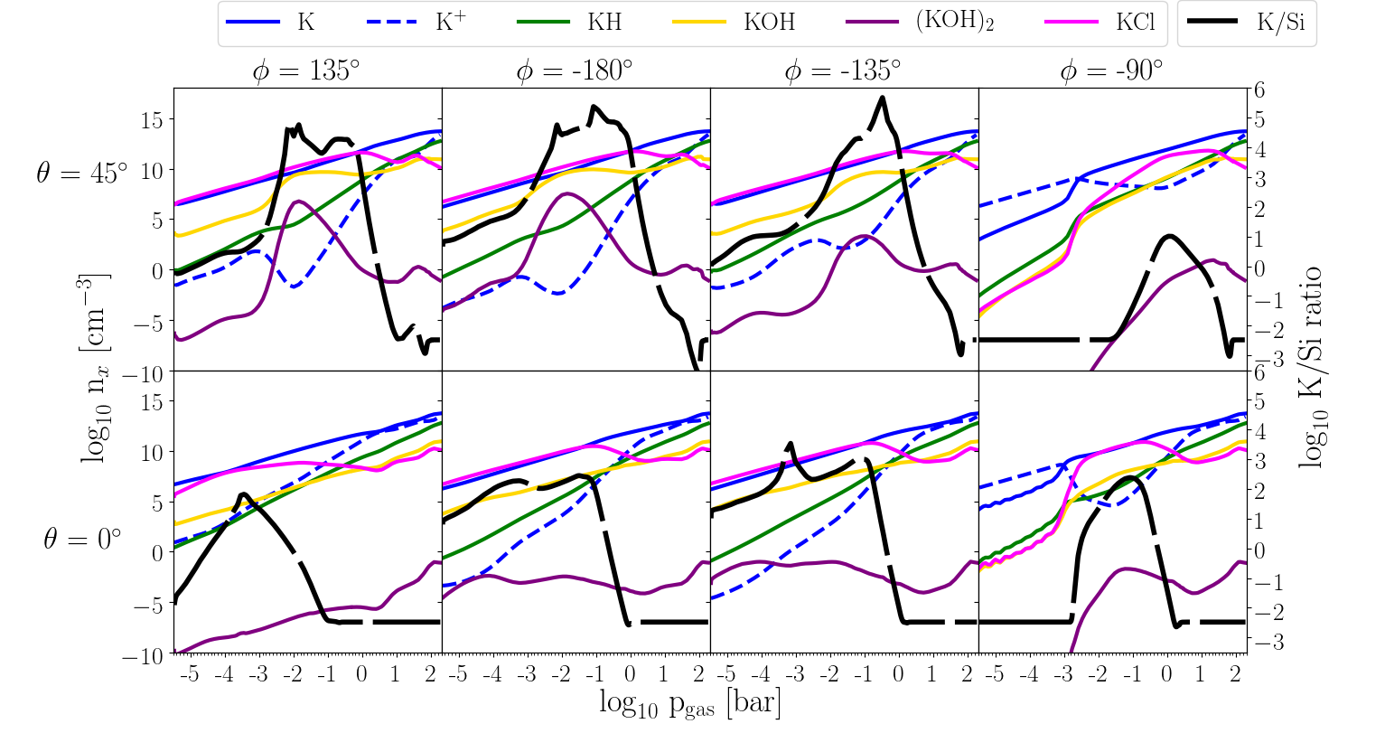
Figure 19: Number densities, log $n_{\rm x}$ [cm^-3], of K-binding gas-species (color coded, left axis). The log(K/Si) ratio is overplotted and shows where cloud affects the atmosphere (black long-dashed line, right axis).

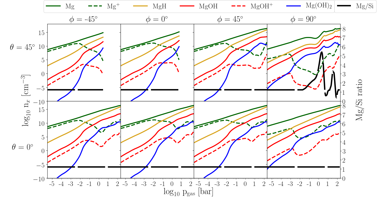
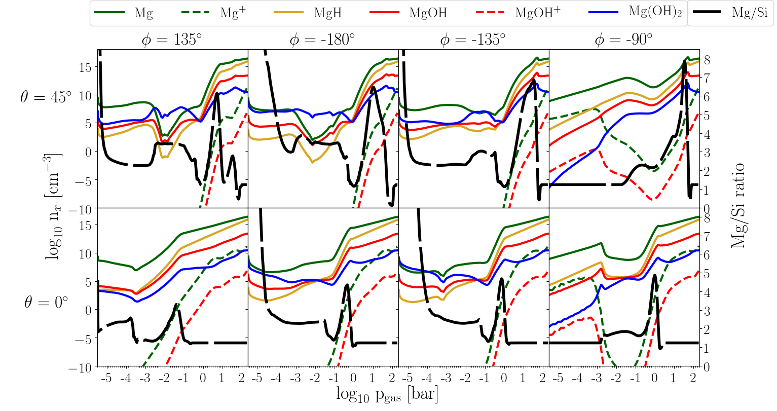
Figure 20: Number densities, log $n_{\rm x}$ [cm^-3], of Mg-binding gas-species (color coded, left axis). The Mg/Si ratio is overplotted and shows where cloud affects the atmosphere (black long-dashed line, right axis).

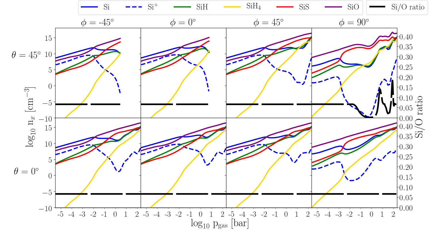
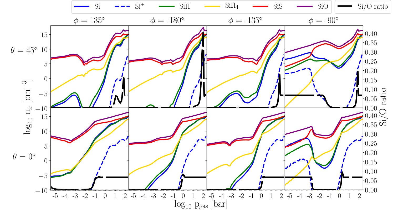
Figure 22: Number densities, log $n_{\rm x}$ [cm^-3], of Si-binding gas-species (color coded, left axis). The Si/O ratio is overplotted and shows where cloud affects the atmosphere (black long-dashed line, right axis).

Similar behaviour occurs for all elements involved in the cloud formation processes and the detailed results for [X/Si] are provided in Appendix A where each figure shows the gas-abundance and the respective X/Si curve (thick, black dashed line). Bedell et al. (2018) show that their Mg/Si for solar twins in the solar neighborhood are greater than one. Our initial, undepleted (Mg/Si)⁰ = 1.23 and cloud formation pushes Mg/Si as high as 8 at the inner cloud boundary at the $\phi=-90^{o}$ terminator (Fig. 20), and well above 4 at the inner cloud boundary of all other cloud-affected profiles probed in our study. Mg and Si are very correlated in the regions where both participate in cloud formation, but the inner, low-altitude cloud regions are more affected by SiO than any Mg-binding condensate. Hence, the large Mg/Si occur where Si is still strongly depleted which is also reflect in the Si/O ratio (Fig. 22). Fe/Si shows similar features in regions where Si is strongly depleted, like in the nucleation zone at $\phi=-134^{o}$ (Fig. 18). In principle, the same story is told by all the other mineral ratios. Examples like K/Si and Na/Si demonstrate very well where the Si depletion kicks in because K and Na are not depleted (Figs. 19, 21) as they do not condense in the temperature regimes of WASP-18b. Consequently, the lowest metalicity gas exhibits the highest Mg/Si. The detailed finding for the mineral ratios are provided in Appendix A.

Woitke et al. (2017) investigated the change of the gas-phase C/O ratio in the limiting case of thermal stability which allows to consider the effect of complex materials like phyllosilicates. Their results demonstrate that the condensation of Mg/Si/O-binding minerals increases C/O to $>0.7$, and that a further increase to $>0.8$ is caused if phylosilicates are included. They also demonstrate that deriving the C/O ratio from a gas only made of H/C/N/O as elements leads to false results compared to the whole set of solar elements.

The changing element ratios demonstrate that an atmospheric ratio (as for C/O, for example) will differ from the bulk value or in fact from any value derived for the warmer, deeper atmospheric regions. The pristine, unaltered atmospheric element ratios should be recovered. An added complication may arise for an extended inner, low-altitude cloud which is enriched by elements (C/O decreases) rather than depleted (C/O increases).

Table 1: An account of the dominating gas-phase species per element for WASP-18b

	Day	Night	Terminators
			Longitude $\phi=-90^{\circ}$	Longitude $\phi=90^{\circ}$
Al	p¡10-2bar: Al+ p¿10-2bar: Al at high $p_{\rm gas}$: AlH, AlOH	AlOH, AlO2H at high $p_{\rm gas}$: Al, Al+	$p_{\rm gas}<10^{-2}$bar: Al $p_{\rm gas}>10^{-2}$bar: AlOH at high $p_{\rm gas}$: Al, AlH, AlOH	Lat $\theta=45^{\circ}$: $p_{\rm gas}<10^{-2}$bar: Al $p_{\rm gas}>10^{-2}$bar: AlOH at high $p_{\rm gas}$: Al, AlH, AlOH. Lat $\theta=0^{\circ}$: $p_{\rm gas}<10^{-3}$bar: Al+ $p_{\rm gas}>10^{-3}$bar: AlH, AlOH at high $p_{\rm gas}$: Al, AlH, AlOH
Ca	$p_{\rm gas}<10^{-2}$bar: Ca+ $p_{\rm gas}>10^{-2}$bar: Ca	$p_{\rm gas}$¡10-3bar: Ca(OH)2, CaCl2 $p_{\rm gas}$=10${}^{-3}...<1$bar: Ca(OH)2 $p_{\rm gas}>$1bar: Ca	Ca if clouds: Ca(OH)2, CaCl2	Ca
C	CO	CO, CH4	CO ; CH4 at high p	CO ; CH4 at high p
Fe	Fe, Fe+	Fe; low $p_{\rm gas}$: Fe(OH)2 high $p_{\rm gas}$: FeH	Fe	Fe
H	$p_{\rm gas}<10^{-1}$bar: H $p_{\rm gas}>10^{-1}$bar: H2	H2; at high $p_{\rm gas}$: H	H2 ; $p_{\rm gas}<10^{-3}$bar : H	H2 ; p¡10-3bar: H
Mg	Mg ; $p_{\rm gas}<10^{-2}$bar: Mg+ (many differences for Mg at each profile)	Lat $\theta=45^{\circ}$: $p_{\rm gas}$¡10-3 &$p_{\rm gas}$¿10-1: Mg $p_{\rm gas}$=10${}^{-3}...10^{-1}$bar: Mg(OH)2 Lat $\theta=0^{\circ}$ : Mg $p_{\rm gas}<10^{-4}$bar: Mg(OH)2 highest $p_{\rm gas}$: MgH	Mg MgH at high $p_{\rm gas}$	Mg MgH at high $p_{\rm gas}$
O	CO, $p_{\rm gas}$¡10-2bar: O $p_{\rm gas}>10^{-2}$bar: H2O	CO, H2O	CO all $p_{\rm gas}$/ $p_{\rm gas}$¿10-3bar: H2O	CO; $p_{\rm gas}>10^{-3}$: H2O
Si	$p_{\rm gas}<10^{-2}$: Si $p_{\rm gas}>10^{-2}$: SiO	SiS, SiO	SiO	SiO
S	low $p_{\rm gas}$: S high $p_{\rm gas}$: H2S	H2S	$p_{\rm gas}<10^{-3}$: S $p_{\rm gas}>10^{-3}$: H2S	$p_{\rm gas}<10^{-3}$: S $p_{\rm gas}>10^{-3}$: H2S
Ti	$p_{\rm gas}<10^{-2}$: Ti+ $p_{\rm gas}>10^{-2}$: Ti, TiO	$p_{\rm gas}<1$bar: TiO2 $p_{\rm gas}>1$bar: TiO highest $p_{\rm gas}$: Ti	TiO TiO2 when clouds form	TiO $p_{\rm gas}<10^{-3}$/ highest $p_{\rm gas}$: Ti

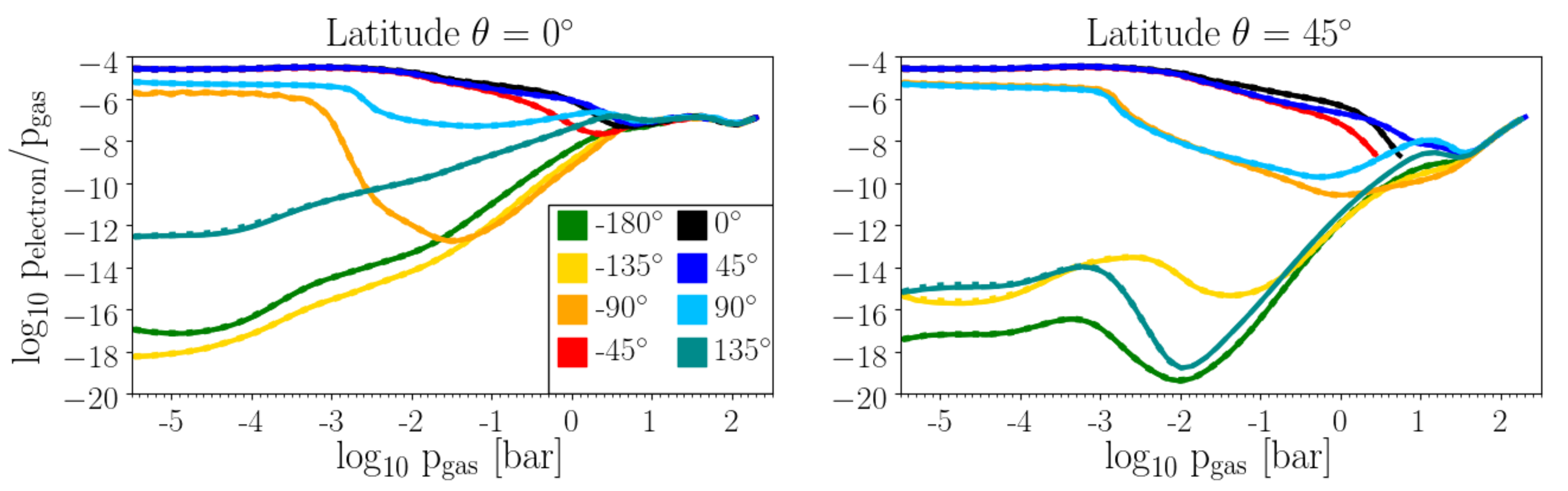
Figure 9: WASP-18b’s dayside ionosphere due to a partially ionised gas in the atmosphere ($\phi=-90^{o},-45^{o},0^{o},45^{o},90^{o}$): The degree of thermal ionisation from the day to the night side at the equator (left) and in the northern hemisphere (right) of WASP-18b. The ionosphere more extended in the equatorial regions ($\theta=0^{o})$ than in northern hemisphere ($\theta=45^{o}$).

4.3 The composition of the neutral gas-phase on WASP-18b

The most direct information about an atmosphere can be derived if gas species can be observed spectroscopically because individual atoms and molecules are finger prints for specific temperature and pressure regimes. Such a direct access is hampered if clouds form, but WASP-18b provides us with a cloud-free dayside. Figures 13- 24 provide a detailed account of the gas-phase composition of the atmosphere of WASP-18b sorted by elements. Each of these plots contains an element ratio (C/O, Si/O, Mg/Si, Na/Si etc.) which allows to trace the cloud forming regions as discussed in Sect. 4.2. Here, we confine ourselves to features of general and also of specific interest in order to build our understanding for the chemical composition in such thermodynamically diverse planets.

The most abundant species of the collisional dominated parts of the atmospheric gas on WASP-18b are in decreasing order H₂, CO, SiO, H₂O, SiS, and MgH on the dayside. This hierarchy changes somewhat on the nightside to: H₂, CO, H₂O, CH₄, H₂S. The most abundant gas-phase species are neutral molecules despite the large temperature difference between day and night (Fig. 8). A summary of dominating gas species is provided in Table 1.

Despite H₂ being the most abundant molecule, it is not everywhere the most abundant H-binding species. This has recently been pointed out by Arcangeli et al. (2018). The dayside of WASP-18b is dominated by atomic hydrogen, H, up to $10^{-2}$bar, and at both day/night terminators up to $10^{-3}$bar (Fig. 13). We note that at the equatorial $\phi=-90^{o}$-terminator, H and H₂ appear with very similar number densities. The nightside is H₂ dominated as the gas temperature is too low for thermally dissociating H₂.

For the O-complex, CO does dominate the gas phase on the dayside, followed by atomic oxygen in the outer layers and by H₂O in regions of high densities. The night side is affected by the thermodynamics of the atmosphere and element depletion of oxygen through the formation of silicates. The drop in CO correlates well with the peak in C/O which indicates efficient cloud formation and it is compensated by an increase of CH₄ and H₂O (see $\phi=-135^{o},-180^{o}$, Fig. 14).

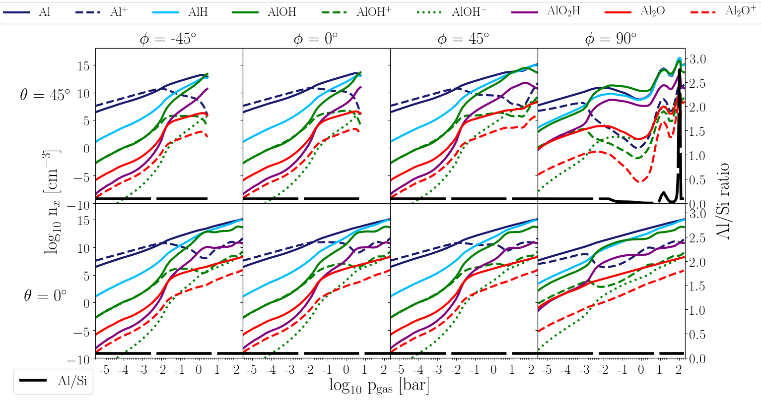
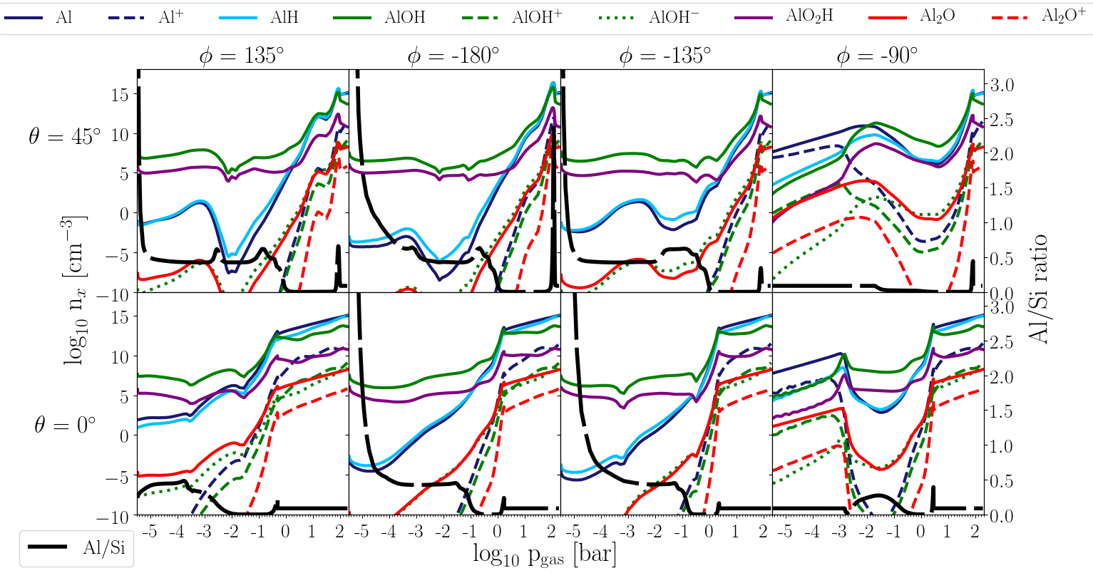
Figure 15: Number densities, log $n_{\rm x}$ [cm^-3], of aluminum binding gas-species (color coded, left axis). The Al/Si ratio is overplotted and shows where cloud affects the atmosphere (black long-dashed line, right axis).

Aluminium and titanium are elements that play a key role for cloud formation as they form materials that are thermally stable up to rather high temperatures compared to Mg/Si/Fe/O-silicates. Both, the Al and the Ti complex (Figs. 15, 24) replicate what is commonly observed for alkali metals (Na, K, Ca): Their positive ions become more abundant than the neutral atom, in fact, than any of their neutral counterparts: The Al-complex (Fig. 15) is dominated by AlH in the high-altitude atmosphere on the nightside, Al⁺/Al at the dayside and Al/AlOH/AlH at the day/night terminator. The equatorial area at $\phi=-90^{o}$ is dominated by atomic aluminium. The Ti-complex (Fig. 24) is dominated by TiO₂ on the nightside ($\phi=135^{o},-180^{o},-135^{o}$), Ti⁺/Ti at the dayside and Ti/TiO at the limbs ($\phi=90^{o},-90^{o}$)

Neither Fe not Si exhibit an ion that is more abundant than any of their neutral atoms or molecules

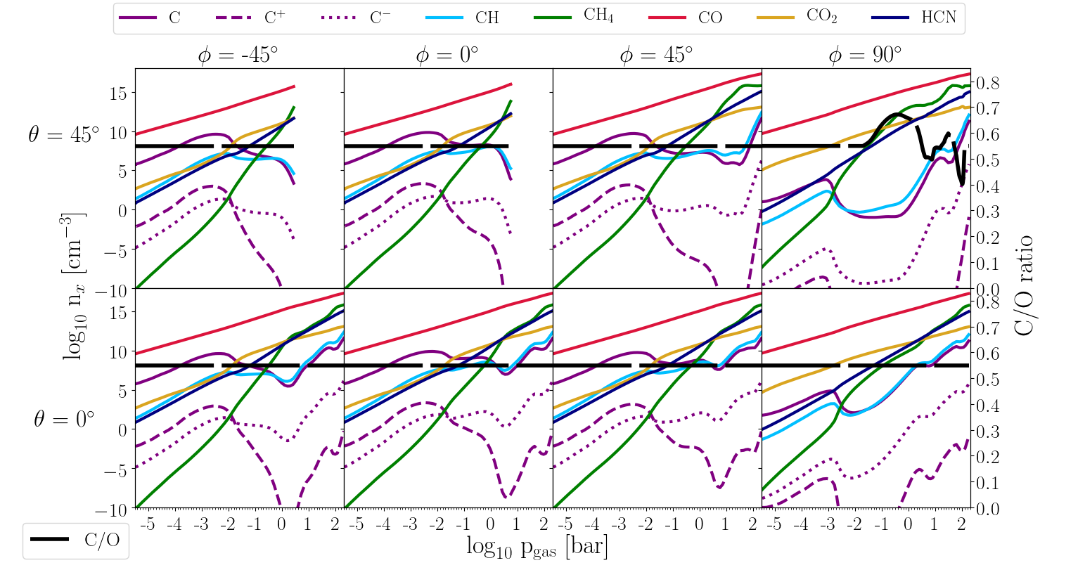
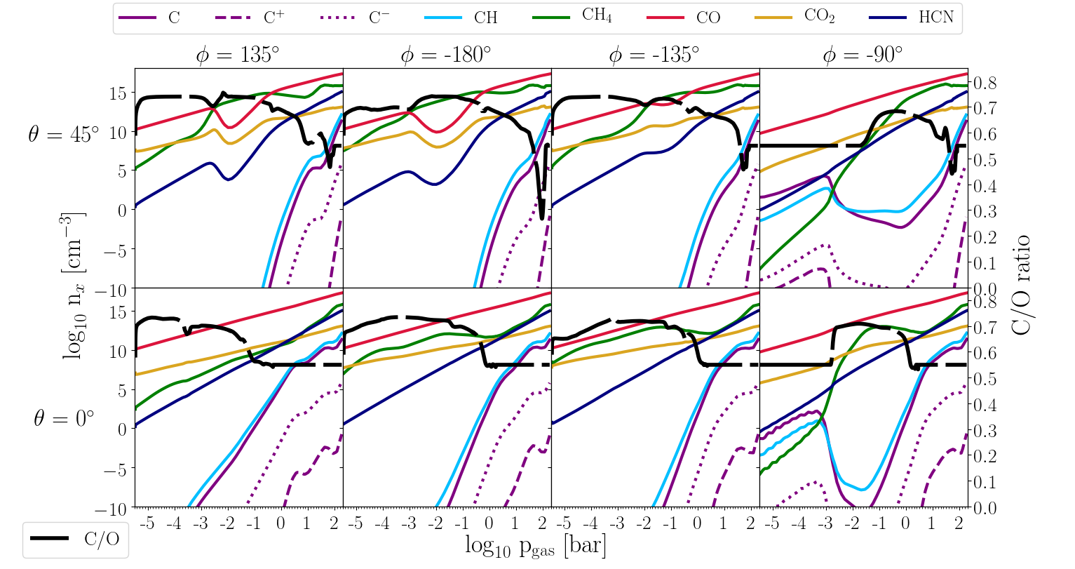
Figure 16: Number densities, log $n_{\rm x}$ [cm^-3], of carbon binding gas-species (color coded, left axis). The C/O is overplotted and shows where cloud affects the atmosphere (black long-dashed line, right axis).

The C-complex is dominated by CO on almost all profiles except for the northern profiles at the nightside (Fig. 16).

Figure 8 demonstrates how profoundly the globally changing thermodynamic structure affects the local molecular number densities (day-night difference) and how strongly the cloud formation affects the actual values (the over plotted C/O serves as guid for the cloud location on the pressure axis) of atoms and molecules.

4.4 The dayside ionosphere of the partially ionised atmosphere of WASP-18b

Brown dwarfs have a long tradition of being studied as analogs for giant gas planets because spectral observations are more feasible than for extrasolar planets (e.g. Charnay et al. 2018). Brown dwarfs irradiated by white dwarfs have recently been discovered and emission lines that origin from heated upper atmospheric regions at high altitudes have been observed from the irradiated brown dwarf WD0137-349B (Longstaff et al. 2017). While the specific ionised species (Fe⁺ vs. Na⁺) observed will be determined by the temperature that can be reached in these hot, outer regions, WASP-18b has a hot enough dayside for atomic ions to emerge.

Ions dominating: The temperature on the day side of WASP-18b is high enough that various elements appear in their second ionisation state (singly ionised) as shown in Fig. 8 (top). The most abundant ions that are also more numerous than the neutral atoms are Na⁺, K⁺, and Ca⁺. Also Al⁺ and Ti⁺ are more abundant than their atomic form (Fig. 15,  24) but are far less numerous than Na⁺, K⁺, or Ca⁺. H^- is far more abundant at the dayside and in the terminator regions than at the nightside, but never the dominating H-species. This supports the finding in Arcangeli et al. (2018). Figure 8 has over-plotted the total electron number density (dark gray) demonstrating that the most important electron donors on the dayside of WASP-18b are Mg, Fe, Al, Ca, Na, and then K. Mg and Fe had been identified as dominating electron donors in the inner, warmest low-altitude parts of non-irradiated giant gas planet and brown dwarf atmospheres (Rodríguez-Barrera et al. 2015).

Possible emission: We note that the atomic hydrogen abundance, as well as that of Al⁺, Ti⁺, and Fe⁺ (and atomic O, C, Si) increases outward where the local temperature increases outwards on WASP-18b. This may suggest that WASP-18b shows emission from H$\alpha$ (and O, C, Si, Al⁺, Ti⁺, Fe⁺) from its dayside and terminator regions. Possible emission lines could include $\lambda=4243.47,\ldots,5262.02,\ldots,7494.75,\ldots,8286.72\AA$ for Fe⁺ (Fe II), $\lambda=6231.06,\ldots,6822.69,\ldots 8925.81\AA$ for Al⁺ (Al II), $\lambda=8445.44\AA$ for O (OI) (e.g. as seen in post-AGB stars by Arkhipova et al. 2018), $\lambda=4571.98,5129.15\AA$ for Ti⁺ (Ti II), $\lambda=8824.221\AA$ for Fe (Fe I) (e.g. as seen in accretion outburst of an M5-dwarf with a protoplanetary disk by Sicilia-Aguilar et al. 2017). The occurrence of these lines will depend on the local temperature and density, and a proper radiative transfers calculation will be required for providing a more profound theoretical support for this suggestion. H$\alpha$ is used as measure for planetary mass loss. The possibility of mass loss on ultra hot Jupiters was discussed in Lothringer et al. (2018) for the hottest example among the super-hot Jupiters, KELT-9b.

Dayside ionosphere on ultra-hot Jupiters: The changing state of thermal ionisation of the individual elements causes a difference of 15 order of magnitudes in the local degree of thermal ionisation, $f_{\rm e}$, between the day and the nightside on WASP-18b (Fig. 9). The nightside is cool enough that only little thermal ionisation occurs in almost the entire vertical atmosphere. The degree of ionisation on the dayside reaches an approximately constant level at $p<10^{-2.5}$bar of $f_{\rm e}\approx 10^{-4.5}$. Most of the high-altitude atmosphere on the dayside and at the day/night terminators has $f_{\rm e}>10^{-7}$. The value of $f_{\rm e}>10^{-7}$ has been suggested to be a threshold above which a gas may exhibit plasma behavior without being fully ionised (Rodríguez-Barrera et al. 2015). Hence, the dayside of WASP-18b can be expected to show plasma phenomena, incl. magnetic field coupling. This conclusion is in line with works on other ultra-hot Jupiters. For example does Kreidberg et al. (2018) conclude that a magnetic drag force is required to explain the phase curve of WASP-103b.

The dayside of WASP-18b reaches temperatures as high as 3500K which is too low to ionised the atomic hydrogen that dominates the daysides high-altitude atmosphere thermally (Fig. 13). The nightside is completely neutral and all elements appear in their first (neutral) state of ionisation. The dayside is composed of a partially ionised gas which has a electron number density comparable to and above Earth’s ionosphere ($10^{6}$cm^-3). We therefore postulate that WASP-18b and other ultra-hot Jupiters like WASP-121b, WASP-12b, WASP-103b, WASP-33b, Kepler-13Ab, Kepler 16b, KOI-13b, MA-1b have an ionosphere on their dayside that stretches into the terminator regions. Planets right of the 20% line in Figure 13 in Parmentier et al. (2018) will fall into this category.

Would the nightside develop an ionosphere, too, for example due to scattered XUV photons from the host star (stellar XUV has a huge effect on the mass loss of small planets; e.g. King et al. 2018) or other high-energy irradiation from e.g. the interplanetary environment? It is reasonable to expect that external radiation increases the ionisation of the atmospheric gas in its upper, high-altitude regions similar to what has been shown for brown dwarfs. A considerable increase of the degree of ionisation results in a thin shell of an almost or fully ionised gas if the irradiation were comparable to the ISM radiation field (Rodriguez-Barrera et al. 2018). Cosmic rays will not significantly contribute to the formation of an ionosphere because they are rather efficiently attenuated (Rimmer & Helling 2013).

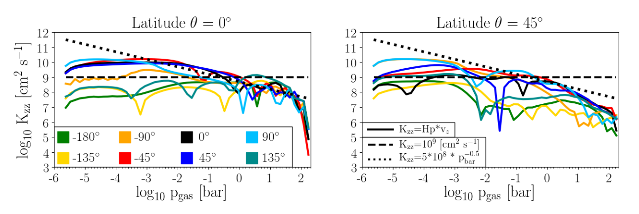
Figure 10: The vertical diffusion coefficient, $K_{\rm zz}$, calculated from various parametrisations: $K_{\rm zz}=H_{\rm p}v_{\rm z}$, $K_{\rm zz}=10^{9}$ cm²s^-1, $K_{\rm zz}=5\cdot 10^{8}p^{-0.5}$ cm² s^-1. The representation $K_{\rm zz}=f(p)$ is the same as derived in Parmentier et al. (2013).

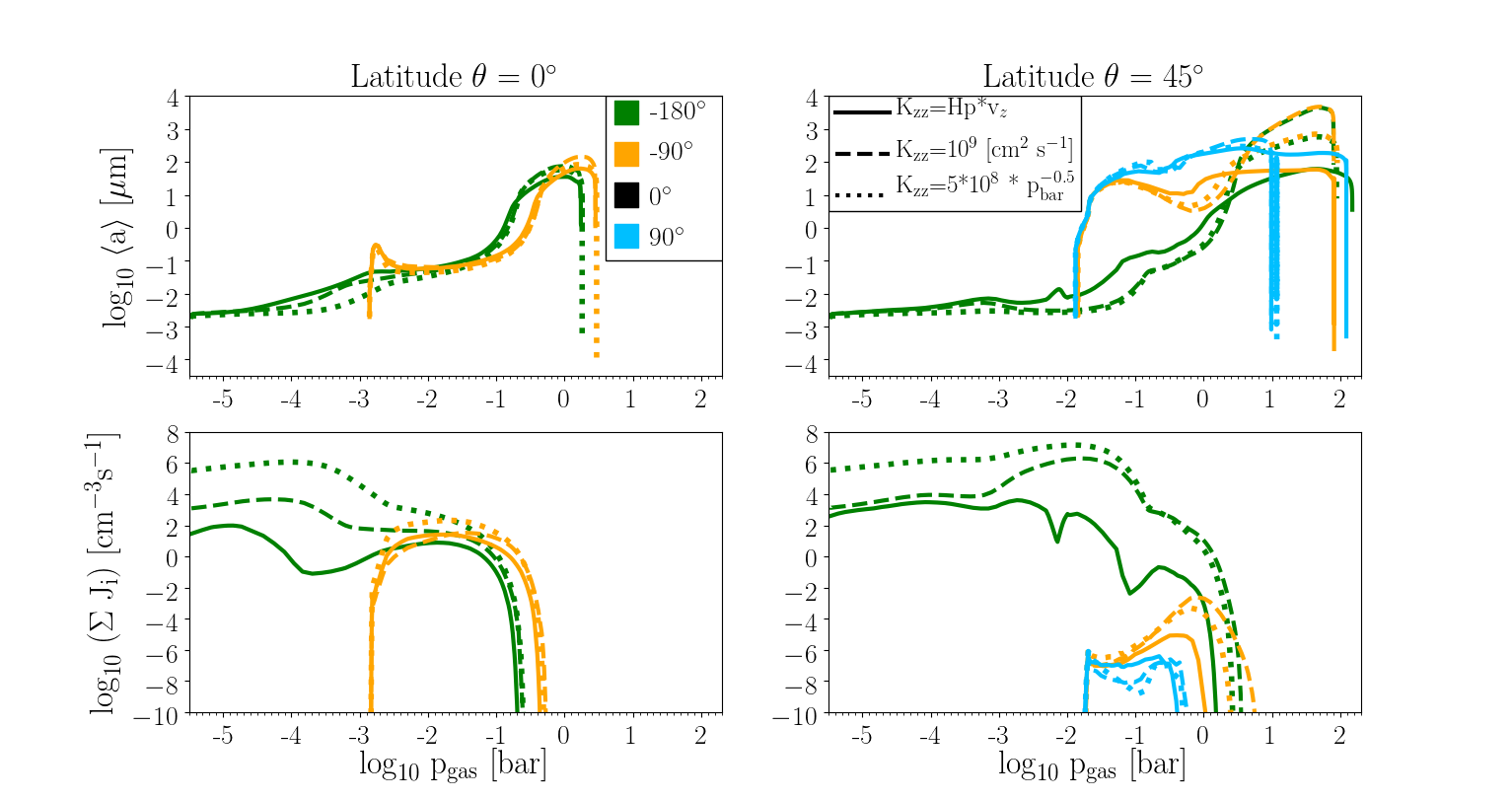
Figure 11: Different element replenishment representations and the nucleation rate, $J_{*}=\Sigma J_{i}$, and the local mean particle size, $\langle a\rangle$, of WASP 18b.

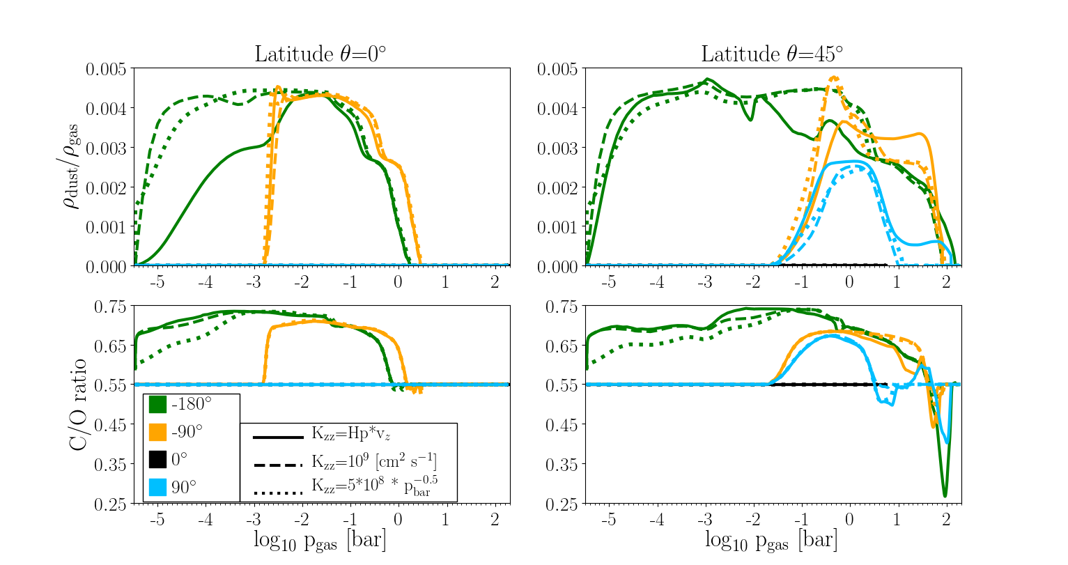
Figure 12: Different element replenishment representations and global cloud properties of WASP-18b: $\rho_{\rm d}/\rho_{\rm gas}$ (top) and C/O ratio (bottom) .

5 Discussion

5.1 Element replenishment representations

The solution of the Navier-Stokes equations in combination with a radiative transfer, gas phase chemistry, element conservation and cloud formation enables a parameter-free solution. Only material properties and numerical parameters remain to be adjusted. Not so in 1D. 1D approaches are numerically fast, hence, can be run on a high cadence as required, for example, in the retrieval approaches (e.g. Blecic et al. 2017). Our cloud formation model provides us with the tool that we need to predict cloud properties based on a fundamental understanding of microphysical processes like cluster formation, frictional interaction, surface reactions. But we have demonstrated that a replenishment mechanism is required to describe cloud formation in a 1D quasi-static atmospheric environment (Woitke & Helling 2004, Appendix A). Therefore, element replenishment is parameterised in 1D cloud simulations. Helling et al. (2008a) and Charnay et al. (2018) summarized the approaches applied in the brown dwarf / giant gas planet literature where $\tau_{\rm mix}\sim H_{\rm p}(z)^{2}/K_{\rm zz}$. Here, we test our classical approach of $K_{\rm zz}=H_{\rm p}v_{\rm z}$ against a constant $K_{\rm zz}=10^{9}$ cm²s^-1 and a scaling with the local pressure $K_{\rm zz}=5\cdot 10^{8}p^{-0.5}$ with p in [bar]. The $K_{\rm zz}$-approach originates from modelling mixing as diffusion process, and the $\tau_{\rm mix}$-approach models mixing as large-scale convection. The $K_{\rm zz}$-scaling with the local gas-pressure was derived from a 3D cloud-free GCM for HD209758b which has a different temperature structure as demonstrated in Fig. 2. Figure 10 shows how the different parameterisations vary for the 1D profiles used here.

Figures 11 show the nucleation rate and the mean cloud particle sizes for the three different $K_{\rm zz}$ parameterisations. Different profiles are shown in different colors, and the different $K_{\rm zz}$ cases are visualised by different line stiles. The cloud results for the day/nightside terminators remain rather unchanged for the three approaches tested because the nucleation rates are very similar. For all other profiles, the largest differences occur to the approach that scales with the local gas pressure (dotted lines). The nucleation rate differs here up to 4 orders of magnitude compared to the constant value (dashed lines). The consequence is that the mean particles sizes vary but just by maximally 1-1.5 order of magnitudes in the inner, low-altitude, hence optically tick cloud. The cloud particle load of the atmosphere reflects this, too.

While it is elusive to discuss which of the approaches could be called ’correct’, the comparison provides some idea about uncertainties that are imposed by differences in $K_{\rm zz}$. We have demonstrated this in terms of cloud particle load, $\rho_{\rm d}/\rho_{\rm gas}$, and in terms of the C/O ratio (Fig. 12). The differences in the mixing/diffusion don’t have much effect on the results at the equatorial, cloud-forming terminator ($\phi=-90^{o}$) and on the northern terminator at $\phi=90^{o}$ regarding $\rho_{\rm d}/\rho_{\rm gas}$ and C/O. The largest uncertainties occur at the high altitudes of the cloudy atmosphere for both, the cloud itself and the feedback on the gas phase.

We note that the three approach give roughly the same answer, but the parametrized Kzz’s give a much smoother variation of parameters like the particle size. Hence, small scale variations in the cloud properties are due to local variations of $K_{\rm zz}=H_{\rm p}v_{\rm z}$ and are possibly not too realistic. Furthermore, horizontal mixing can not be considered in the approach followed in this paper, but will homogenize the global element abundance and cloud particle distribution to a certain extend in the higher altitude regions where the gas pressure is low if the wind blows into the right direction (night $\rightarrow$ day) and thermally stability prevails. For example, the cloud particle size differences between the equator and the mid-latitudes, and the limb and the anti-stellar point would be lessened if the gas is supersaturated. For WASP-18b, the dayside will remain cloud free as no material achieves supersaturation for temperatures as high as $>2200$K (Woitke et al. 2017). This condition worthens with decreasing pressure. It will therefore be essential to measure the atmospheric C/O on the day and on the nightside in order to link the atmospheric C/O to the bulk C/O of extrasolar planets.

5.2 Comparing WASP-18b to HD 189733b and HD 209458b

Despite the limits to our approach, we can offer some general comparisons between the three giant gas planets that we have studied so far with respect to cloud formation and chemistry feedback. This comparisons should not go into details as the 3D models for HD 189733b and HD 209458b take the clouds consistently into account for the gas-phase chemistry and for the radiative transfer, while this is not yet the case for WASP-18b.

WASP-18b with $T_{\rm eq}\approx 2400$K is far hotter than HD 189733b and HD 209458b with $T_{\rm eq}\approx 1000$K and $T_{\rm eq}\approx 1500$K, respectively, and its surface gravity is one order of magnitude larger. Figure 2 shows, that despite these substantial differences in global parameters, the night side of all three giant gas planets exhibit very comparable temperatures. And all three planets develop temperature inversions on their dayside (rather shallow in HD 209458b). In the low-pressure regions of the nightside profiles, WASP-18b has higher pressures for any given local gas temperature. Higher pressures enable condensation processes at higher temperatures as thermal stability expands into higher temperature regimes with increasing pressure.

The overall material composition of the cloud particles are very similar in all three planets, though differences do emerge in the details. The high-altitude atmosphere is dominated by Mg/Si/O-materials with $\approx 15$% of Fe[s]. The nucleation species determine the composition of the thin, uppermost cloud boundary. WASP-18b has a distinct SiO[s] layer where Mg/Si/O-materials have evaporated. This SiO[s] layer does not appear in HD 189733b and HD 209458b.

The overall mean particle sizes are comparable and span a similar range in all three planets. The actual height-dependent size distribution does vary between the planets. For example WASP-18b’s $\phi=-90^{o}$-terminator show only very minimal changes of cloud particles sizes with height compared to all other profiles sampled. Here the material matrix is dominated by SiO[s] over most of the cloud volume, except at the cloud top where distinct layers of Fe[s] and CaTiO₂[s] appear.

The total vertical cloud extension reaches farther into the low-pressure atmosphere on WASP-18b despite having a surface gravity that is one order of magnitude larger than that of HD 189733b. HD 209458b has clouds that reach into the lowest pressure regimes: The upper nightside cloud boundary is located at $p_{\rm gas}\approx 10^{-5.5}$bar on WASP-18b, at $p_{\rm gas}\approx 10^{-4.2}$bar on HD 189733b and at $p_{\rm gas}\approx 10^{-7}\,...\,10^{-5}$bar on HD 209458b (compare Fig. 4 and Fig. 8 in Helling et al. (2016)). Our test of mixing prescriptions in Sect. 5.1 suggests that the upper cloud boundary is not affected by mixing here and is hence determined by the local thermodynamic conditions.

6 Conclusion

WASP-18b provides us with a laboratory to study the atmosphere chemistry of ultra-hot Jupiters that have very hot days and cold nights.

Hot Jupiters do not have all their constituents in the gas phase, and cloud formation strongly affects the chemistry on the nightside and on the day/night terminators. The WASP-18b dayside is hot enough to thermally dissociate H₂, and the elements Na, K, Ca, Ti, Al as well as Fe, Mg, Si but to a lesser degree. VO, TiO and H₂O are not among the most abundant gas-phase species on the dayside which is in line with the non-detection in HST secondary eclipse observations. TiO and H₂O are important for gas pressures above 10^-2 bar on the dayside. The low-density regime of the dayside has CO but also atomic species like Si and S, and ions like Na⁺, Ca⁺, K⁺. The low-pressure regime of the terminator gas-phase chemistry is made of bi-atomic molecules like CO, SiO, TiO and atoms like for example Fe and Mg. We further find that:

• WASP-18b has two very different sides: The nightside is cloudy and element depleted, the dayside is cloud-free and forms a thermal ionosphere that reached deep into the atmosphere.

• The largest cloud particles form at the $\phi=-90^{o}$ (west) day/night terminator, and superrotation causes a cloud-free $\phi=90^{o}$ (east) day/night terminator.

• Clouds become more extended towards the west of the nightside. Clouds are located farther inside the atmosphere and less extended at the limbs compared to the nightside.

• The cloud particle load (dust-to-gas-ratio $\rho_{\rm d}/\rho_{\rm gas}$) is rather homogeneous of the order of $10^{-3}$ despite large temperature difference in the cloud forming regions of WASP-18b.

• Element enrichment occurs deep inside the atmosphere and the observable layers appear depleted in all elements that participate in cloud formation.

• At the dayside, where no cloud formation happens, the atmospheric C/O is constant and remains at its undepleted value (here: solar). In the nightside, C/O is roughly constant but enhanced (C/O$\sim$0.7) within the photosphere. At the limbs the C/O ratio varies vertically from 0.7 to 0.5 within the layers probed by transmission spectroscopy. Cloud formation does enhance the C/O in general.

• The cloud particles are made of a mix of materials that changes depending on the local temperature in the atmosphere. The mix is predominantly made of O-binding minerals, smaller oxides or iron, but 5-10% of carbon can be mixed in occasionally. The cloud particles sizes change with height and location.

• The molecular number densities vary by orders of magnitudes between the day and the nightside, and the limbs.

Appendix A Details on chemical composition

Here we provide the detailed composition of the gas-phase in chemical equilibrium for the eight profiles probed at the equator and in the northern hemisphere. We note that GCM models are north/south symmetric such that the southern hemisphere shows the same behavior like the northern hemisphere.

We first provide an overview of how the abundances of the dominating molecular species change (Fig. LABEL:mols) along the equator on the day- and the night side. Figures 14 – 24 detail the chemical gas-phase composition with respect to the individual elements H, O, Al, C, Ca, Fe, Mg, Si, S, Ti. Each of these plots (Figs 14– 24) also shows an element ratio (mineralogical ratios) at the right axis (Al/Si, C/O, Ca/Si, Fe/Si, Mg/Si, Si/O, S/Si, Ti/Si).

Table 2: Solar element abundances, $\epsilon^{0}$ (Asplund et al. 2009), and the solar mineral rations [X/Si]=$\epsilon^{0}_{\rm X}/\epsilon^{0}_{\rm Si}$, Si/O and C/O. Bedell et al. (2018) and Bond et al. (2010) cite Mg/Si=1.05 based on the element abundance data from Asplund et al. (2005) with $\epsilon^{0}_{\rm Mg}=7.53$.

	$\epsilon^{0}$		$\epsilon^{0}_{\rm X}/\epsilon^{0}_{\rm Si,O}$
H	1.000	H/Si	3.0902$\cdot 10^{4}$
He	8.511$\cdot 10^{-2}$	He/Si	2.6301e3
Li	1.122$\cdot 10^{-11}$	Li/Si	3.4672$\cdot 10^{-7}$
C	2.692$\cdot 10^{-4}$	C/Si	8.3189
N	6.761$\cdot 10^{-5}$	N/Si	2.0893
O	4.898$\cdot 10^{-4}$	O/Si	1.5136e1
Na	1.738$\cdot 10^{-6}$	Na/Si	5.3708$\cdot 10^{-2}$
Mg	3.981$\cdot 10^{-5}$	Mg/Si	1.2302
Al	2.818$\cdot 10^{-6}$	Al/Si	8.7082$\cdot 10^{-2}$
S	1.318$\cdot 10^{-5}$	S/Si	0.40729
Cl	3.162$\cdot 10^{-7}$	Cl/Si	9.7713$\cdot 10^{-3}$
K	1.072$\cdot 10^{-7}$	K/Si	3.3127$\cdot 10^{-3}$
Ca	2.188$\cdot 10^{-6}$	Ca/Si	6.7614$\cdot 10^{-2}$
Ti	8.913$\cdot 10^{-8}$	Ti/Si	2.7543$\cdot 10^{-3}$
Fe	3.162$\cdot 10^{-5}$	Fe/Si	9.7713$\cdot 10^{-1}$
Si	3.236$\cdot 10^{-5}$	Si/Si	1
		C/O	0.5495
		Si/O	6.6067$\cdot 10^{-2}$

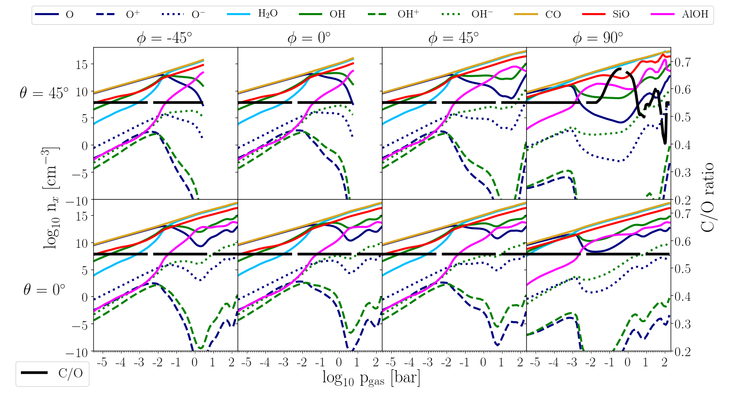
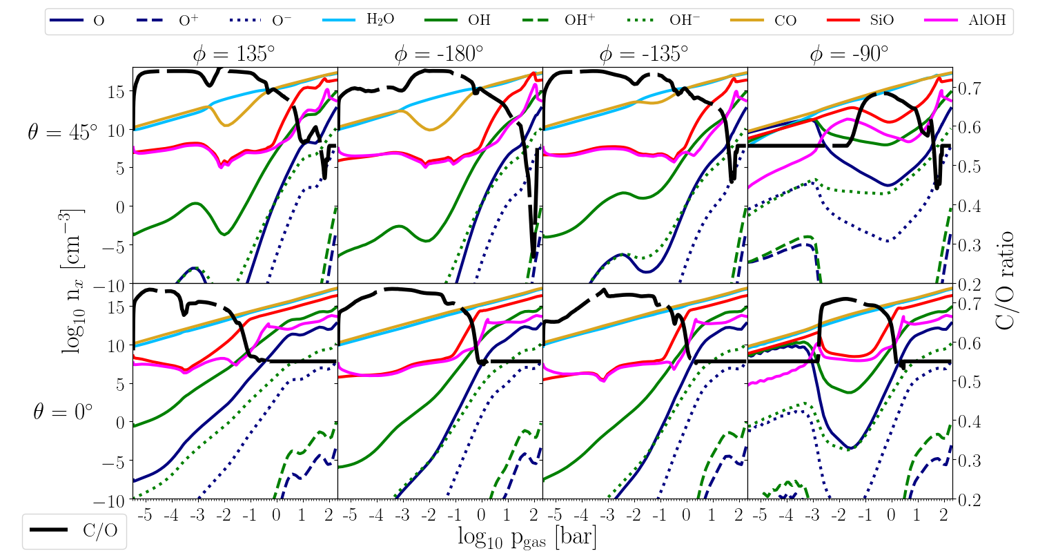
Figure 14: Number densities, log $n_{\rm x}$ [cm^-3], of O-binding gas-species (color coded, left axis). The C/O is overplotted and shows where cloud affects the atmosphere (black long-dashed line, right axis).

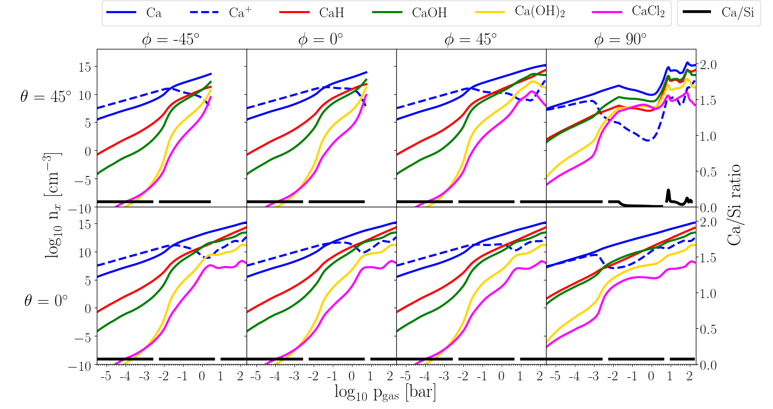
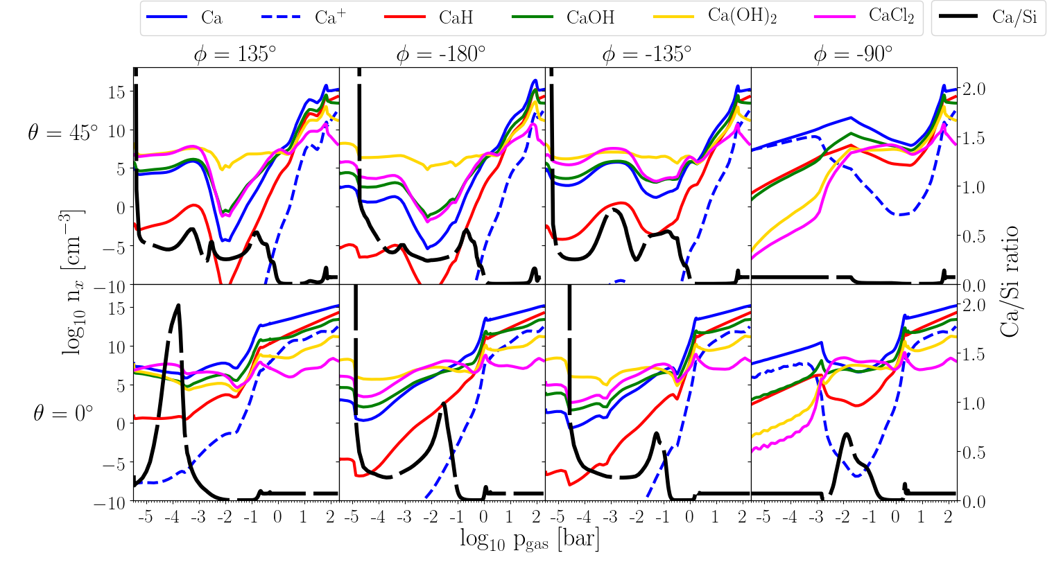
Figure 17: Number densities, log $n_{\rm x}$ [cm^-3], of Ca-binding gas-species (color coded, left axis). The Ca/Si ratio is overplotted and shows where cloud affects the atmosphere (black long-dashed line, right axis).

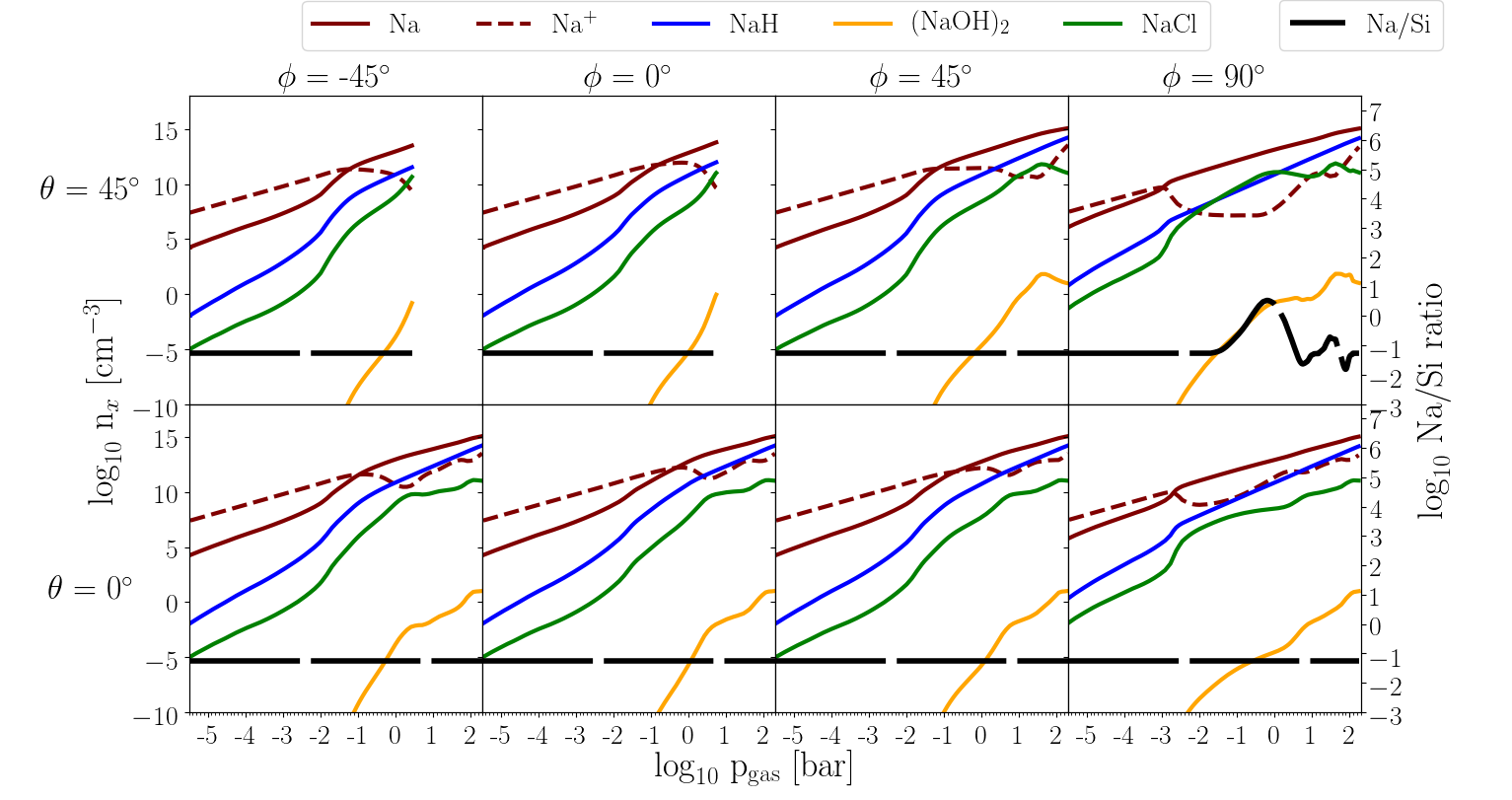
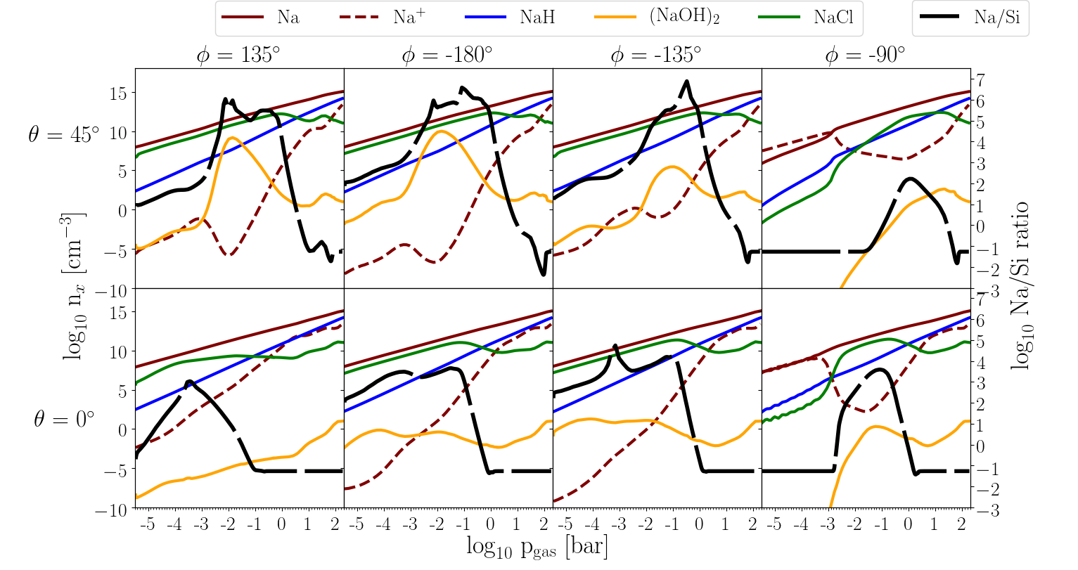
Figure 21: Number densities, log $n_{\rm x}$ [cm^-3], of Na-binding gas-species (color coded, left axis). The log(Na/Si) ratio is overplotted and shows where cloud affects the atmosphere (black long-dashed line, right axis).

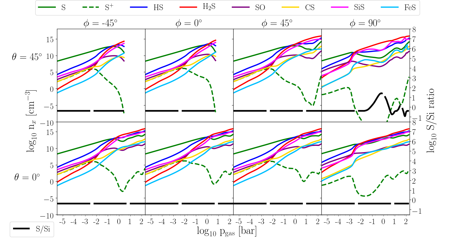
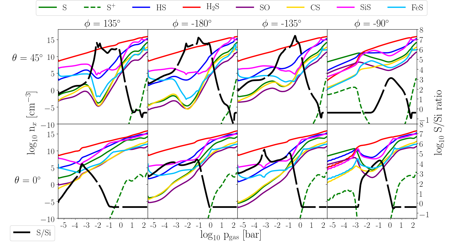
Figure 23: Number densities, log $n_{\rm x}$ [cm^-3], of S-binding gas-species (color coded, left axis). The log(S/Si) ratio is overplotted and shows where cloud affects the atmosphere (black long-dashed line, right axis).

Appendix B Input details

Table 3: Chemical surface reactions $r$ assumed to form the solid materials s. The efficiency of the reaction is limited by the collision rate of the key species, which has the lowest abundance among the reactants. The notation ${\scriptstyle{}^{1}\!\!/\!{}_{2}}$ in the r.h.s. column means that only every second collision (and sticking) event initiates one reaction. Data sources for the supersaturation ratios (and saturation vapor pressures): (1) Helling & Woitke (2006); (2) Nuth & Ferguson (2006); (3) Sharp & Huebner (1990); (4) Woitke et al. (2017)

Index $r$	Solid s	Surface reaction	Key species
1	TiO2[s]	TiO2 $\longrightarrow$ TiO2[s]	TiO2
2	rutile	Ti + 2 H2O $\longrightarrow$ TiO2[s] + 2 H2	Ti
3	(1)	TiO + H2O $\longrightarrow$ TiO2[s] + H2	TiO
4		TiS + 2 H2O $\longrightarrow$ TiO2[s] + H2S + H2	TiS
5	SiO2[s]	SiH + 2 H2O $\longrightarrow$ SiO2[s] + 2 H2 + H	SiH
6	silica	SiO + H2O $\longrightarrow$ SiO2[s] + H2	SiO
7	(3)	SiS + 2 H2O $\longrightarrow$ SiO2[s] + H2S + H2	SiS
8	SiO[s]	SiO $\longrightarrow$ SiO[s]	SiO
9	silicon mono-oxide	2 SiH + 2 H2O $\longrightarrow$ 2 SiO[s] + 3 H2	SiH
10	(2)	SiS + H2O $\longrightarrow$ SiO[s] + H2S	SiS
11	Fe[s]	Fe $\longrightarrow$ Fe[s]	Fe
12	solid iron	FeO + H2 $\longrightarrow$ Fe[s] + H2O	FeO
13	(1)	FeS + H2 $\longrightarrow$ Fe[s] + H2S	FeS
14		Fe(OH)2 + H2 $\longrightarrow$ Fe[s] + 2 H2O	Fe(OH)2
15		2 FeH $\longrightarrow$ 2 Fe[s] + H2	FeH
16	FeO[s]	FeO $\longrightarrow$ FeO[s]	FeO
17	iron (II) oxide	Fe + H2O $\longrightarrow$ FeO[s] + H2	Fe
18	(3)	FeS + H2O $\longrightarrow$ FeO[s] + H2S	FeS
19		Fe(OH)2 $\longrightarrow$ FeO[s] + H2	Fe(OH)2
20		2 FeH + 2 H2O $\longrightarrow$ 2 FeO[s] + 3 H2	FeH
21	FeS[s]	FeS $\longrightarrow$ FeS[s]	FeS
22	iron sulphide	Fe + H2S $\longrightarrow$ FeS[s] + H2	Fe
23	(3)	FeO + H2S $\longrightarrow$ FeS[s] + H2O	$\min\{$FeO, H2S$\}$
24		Fe(OH)2 + H2S $\longrightarrow$ FeS[s] + 2 H2O	$\min\{$Fe(OH)2, H2S$\}$
25		2 FeH + 2 H2S $\longrightarrow$ 2 FeS[s] + 3 H2	$\min\{$FeH, H2S$\}$
26	Fe2O3[s]	2 Fe + 3 H2O $\longrightarrow$ Fe2O3[s] + 3 H2	${\scriptstyle{}^{1}\!\!/\!{}_{2}}$Fe
27	iron (III) oxide	2 FeO + H2O $\longrightarrow$ Fe2O3[s] + H2	${\scriptstyle{}^{1}\!\!/\!{}_{2}}$FeO
28	(3)	2 FeS + 3 H2O $\longrightarrow$ Fe2O3[s] + 2 H2S + H2	${\scriptstyle{}^{1}\!\!/\!{}_{2}}$FeS
29		2 Fe(OH)2 $\longrightarrow$ Fe2O3[s] + H2O + H2	${\scriptstyle{}^{1}\!\!/\!{}_{2}}$Fe(OH)2
30		2 FeH + 3 H2O $\longrightarrow$ Fe2O3[s] + 4 H2	${\scriptstyle{}^{1}\!\!/\!{}_{2}}$FeH
31	MgO[s]	Mg + H2O $\longrightarrow$ MgO[s] + H2	Mg
32	periclase	2 MgH + 2 H2O $\longrightarrow$ 2 MgO[s] + 3 H2	${\scriptstyle{}^{1}\!\!/\!{}_{2}}$MgH
33	(3)	2 MgOH $\longrightarrow$ 2 MgO[s] + H2	${\scriptstyle{}^{1}\!\!/\!{}_{2}}$MgOH
34		Mg(OH)2 $\longrightarrow$ MgO[s] + H2O	Mg(OH)2
35	MgSiO3[s]	Mg + SiO + 2 H2O $\longrightarrow$ MgSiO3[s] + H2	$\min\{$Mg, SiO$\}$
36	enstatite	Mg + SiS + 3 H2O $\longrightarrow$ MgSiO3[s] + H2S + 2 H2	$\min\{$Mg, SiS$\}$
37	(3)	2 Mg + 2 SiH + 6 H2O $\longrightarrow$ 2 MgSiO3[s] + 7 H2	$\min\{$Mg, SiH$\}$
38		2 MgOH + 2 SiO + 2 H2O $\longrightarrow$ 2 MgSiO3[s] + 3 H2	$\min\{{\scriptstyle{}^{1}\!\!/\!{}_{2}}$MgOH, ${\scriptstyle{}^{1}\!\!/\!{}_{2}}$SiO$\}$
39		2 MgOH + 2 SiS + 4 H2O $\longrightarrow$ 2 MgSiO3[s] + 2 H2S + 3 H2	$\min\{{\scriptstyle{}^{1}\!\!/\!{}_{2}}$MgOH, ${\scriptstyle{}^{1}\!\!/\!{}_{2}}$SiS$\}$
40		MgOH + SiH + 2 H2O $\longrightarrow$ MgSiO3[s] + 3 H2	$\min\{{\scriptstyle{}^{1}\!\!/\!{}_{2}}$MgOH, ${\scriptstyle{}^{1}\!\!/\!{}_{2}}$SiH$\}$
41		Mg(OH)2 + SiO $\longrightarrow$ 2 MgSiO3[s] + H2	$\min\{$Mg(OH)2, SiO$\}$
42		Mg(OH)2 + SiS + H2O $\longrightarrow$ MgSiO3[s] + H2S+ H2	$\min\{$Mg(OH)2, SiS$\}$
43		2 Mg(OH)2 + 2 SiH + 2 H2O $\longrightarrow$ 2 MgSiO3[s] + 5 H2	$\min\{$Mg(OH)2, SiH$\}$
44		2 MgH + 2 SiO + 4 H2O $\longrightarrow$ 2 MgSiO3[s]+ 5 H2	$\min\{$MgH, SiO$\}$
45		2 MgH + 2 SiS + 6 H2O $\longrightarrow$ 2 MgSiO3[s]+ 2 H2S + 5 H2	$\min\{$MgH, SiS$\}$
46		MgH + SiH + 3 H2O $\longrightarrow$ MgSiO3[s]+ 4 H2	$\min\{$MgH, SiH$\}$
47	Mg2SiO4[s]	2 Mg + SiO + 3 H2O $\longrightarrow$ Mg2SiO4[s] + 3 H2	$\min\{{\scriptstyle{}^{1}\!\!/\!{}_{2}}$Mg, SiO$\}$
48	forsterite	2 MgOH + SiO + H2O $\longrightarrow$ Mg2SiO4[s] + 2 H2	$\min\{{\scriptstyle{}^{1}\!\!/\!{}_{2}}$MgOH, SiO$\}$
49	(3)	2 Mg(OH)2 + SiO $\longrightarrow$ Mg2SiO4[s] + H2O + H2	$\min\{{\scriptstyle{}^{1}\!\!/\!{}_{2}}$Mg(OH)2, SiO$\}$
50		2 MgH + SiO + 3 H2O $\longrightarrow$ Mg2SiO4[s] + 4 H2	$\min\{{\scriptstyle{}^{1}\!\!/\!{}_{2}}$MgH, SiO$\}$
51		2 Mg + SiS + 4 H2O $\longrightarrow$ Mg2SiO4[s] + H2S + 3 H2	$\min\{{\scriptstyle{}^{1}\!\!/\!{}_{2}}$Mg, SiS}
52		2 MgOH + SiS + 2 H2O $\longrightarrow$ Mg2SiO4[s] + H2S + 2 H2	$\min\{{\scriptstyle{}^{1}\!\!/\!{}_{2}}$MgOH, SiS}
53		2 Mg(OH)2 + SiS $\longrightarrow$ Mg2SiO4[s] + H2 + H2S	$\min\{{\scriptstyle{}^{1}\!\!/\!{}_{2}}$Mg(OH)2, SiS}
54		2 MgH + SiS + 4 H2O $\longrightarrow$ Mg2SiO4[s] + H2S + 4 H2	$\min\{{\scriptstyle{}^{1}\!\!/\!{}_{2}}$MgH, SiS$\}$
55		4 Mg + 2 SiH + 8 H2O $\longrightarrow$ 2 Mg2SiO4[s] + 9 H2	$\min\{{\scriptstyle{}^{1}\!\!/\!{}_{2}}$Mg, SiH}
56		4 MgOH + 2 SiH + 4 H2O $\longrightarrow$ 2 Mg2SiO4[s] + 7 H2	$\min\{{\scriptstyle{}^{1}\!\!/\!{}_{2}}$MgOH, SiH}
57		4 Mg(OH)2 + 2 SiH $\longrightarrow$ 2 Mg2SiO4[s] + 5 H2	$\min\{{\scriptstyle{}^{1}\!\!/\!{}_{2}}$Mg(OH)2, SiH}
58		4 MgH + 2 SiH + 8 H2O $\longrightarrow$ 2 Mg2SiO4[s] + 11 H2	$\min\{{\scriptstyle{}^{1}\!\!/\!{}_{2}}$MgH, SiS$\}$
59	Al2O3[s]	2 Al + 3 H2O $\longrightarrow$ Al2O3[s] + 3 H2	${\scriptstyle{}^{1}\!\!/\!{}_{2}}$Al
60	aluminia	2 AlOH + H2O $\longrightarrow$ Al2O3[s] + 2 H2	${\scriptstyle{}^{1}\!\!/\!{}_{2}}$AlOH
61	(3)	2 AlH + 3 H2O $\longrightarrow$ Al2O3[s] + 4 H2	${\scriptstyle{}^{1}\!\!/\!{}_{2}}$AlH
62		Al2O + 2 H2O $\longrightarrow$ Al2O3[s] + 2 H2	Al2O
63		2 AlO2H $\longrightarrow$ Al2O3[s] + H2O	${\scriptstyle{}^{1}\!\!/\!{}_{2}}$AlO2H

Table 4: Table 3 continued

Index $r$	Solid s	Surface reaction	Key species
64	CaTiO3[s]	Ca + Ti + 3 H2O $\longrightarrow$ CaTiO3[s] + 3 H2	$\min\{$Ca, Ti$\}$
65	perovskite	Ca + TiO + 2 H2O $\longrightarrow$ CaTiO3[s] + 2 H2	$\min\{$Ca, TiO$\}$
66	(3)	Ca + TiO2 + H2O $\longrightarrow$ CaTiO3[s] + H2	$\min\{$Ca, TiO${}_{2}\}$
67		Ca + TiS + 3 H2O $\longrightarrow$ CaTiO3[s] + H2S + 2 H2	$\min\{$Ca, TiS$\}$
68		CaO + Ti + 2 H2O $\longrightarrow$ CaTiO3[s] + 2 H2	$\min\{$CaO, Ti$\}$
69		CaO + TiO + H2O $\longrightarrow$ CaTiO3[s] + H2	$\min\{$CaO, TiO$\}$
70		CaO + TiO2 $\longrightarrow$ CaTiO3[s]	$\min\{$CaO, TiO${}_{2}\}$
71		CaO + TiS + 2 H2O $\longrightarrow$ CaTiO3[s] + H2S + H2	$\min\{$CaO, TiO$\}$
72		CaS + Ti + 3 H2O $\longrightarrow$ CaTiO3[s] + H2S + H2	$\min\{$CaS, Ti$\}$
73		CaS + TiO + 2 H2O $\longrightarrow$ CaTiO3[s] + H2S + 2 H2	$\min\{$CaS, TiO$\}$
74		CaS + TiO2 + H2O $\longrightarrow$ CaTiO3[s] + H2S	$\min\{$CaS, TiO${}_{2}\}$
75		CaS + TiS + 3 H2O $\longrightarrow$ CaTiO3[s] + 2 H2S + H2	$\min\{$CaS, TiO$\}$
76		Ca(OH)2 + Ti + H2O $\longrightarrow$ CaTiO3[s] + 2 H2	$\min\{$Ca(OH)2, Ti$\}$
77		Ca(OH)2 + TiO $\longrightarrow$ CaTiO3[s] + H2	$\min\{$Ca(OH)2, TiO$\}$
78		Ca(OH)2 + TiO2 $\longrightarrow$ CaTiO3[s] + H2O	$\min\rm\{Ca(OH)_{2},TiO_{2}\}$
79		Ca(OH)2 + TiS + H2O $\longrightarrow$ CaTiO3[s] + H2S + H2	$\min\{$Ca(OH)2, TiO$\}$
80		2 CaH + 2 Ti + 6 H2O $\longrightarrow$ 2 CaTiO3[s] + 7 H2	$\min\{$CaH, Ti$\}$
81		2 CaH + 2 TiO + 4 H2O $\longrightarrow$ 2 CaTiO3[s] + 5 H2	$\min\{$CaH, TiO$\}$
82		2 CaH + 2 TiO2 + 2 H2O $\longrightarrow$ 2 CaTiO3[s] + 3 H2	$\min\{$CaH, TiO2 $\}$
83		2 CaH + 2 TiS + 6 H2O $\longrightarrow$ 2 CaTiO3[s] + 2 H2S +5 H2	$\min\{$CaH, TiS$\}$
84		2 CaOH + 2 Ti + 4 H2O $\longrightarrow$ 2 CaTiO3[s] + 5 H2	$\min\{$CaOH, Ti$\}$
85		2 CaOH + 2 TiO + 2 H2O $\longrightarrow$ 2 CaTiO3[s] + 3 H2	$\min\{$CaOH, TiO$\}$
86		2 CaOH + 2 TiO2 $\longrightarrow$ 2 CaTiO3[s] + H2	$\min\{$CaOH, TiO2 $\}$
87		2 CaOH + 2 TiS + 4 H2O $\longrightarrow$ 2 CaTiO3[s] + 2 H2S + 3 H2	$\min\{$CaOH, TiS$\}$
88	CaSiO3[s]	Ca + SiO + 2 H2O $\longrightarrow$ CaSiO3[s] + 2 H2	$\min\{$Ca, SiO$\}$
89	Wollastonite	Ca + SiS + 3 H2O $\longrightarrow$ CaSiO3[s] + H2S + 2 H2	$\min\{$Ca, SiS$\}$
90	(4)	2 Ca + 2 SiH + 6 H2O $\longrightarrow$ 2 CaSiO3[s] + 7 H2	$\min\{$Ca, SiH$\}$
91		CaO + SiO + 1 H2O $\longrightarrow$ CaSiO3[s] + H2	$\min\{$CaO, SiO$\}$
92		CaO + SiS + 2 H2O $\longrightarrow$ CaSiO3[s] + H2S + H2	$\min\{$CaO, SiS$\}$
93		2 CaO + 2 SiH + 4 H2O $\longrightarrow$ 2 CaSiO3[s] + 5 H2	$\min\{$CaO, SiH$\}$
94		CaS + SiO + 2 H2O $\longrightarrow$ CaSiO3[s] + H2S + H2	$\min\{$CaS, SiO$\}$
95		CaS + SiS + 3 H2O $\longrightarrow$ CaSiO3[s] + 2 H2S + H2	$\min\{$CaS, SiS$\}$
96		2 CaS + 2 SiH + 6 H2O $\longrightarrow$ 2 CaSiO3[s] + 2 H2S + 5 H2	$\min\{$CaS, SiH$\}$
97		2 CaOH + 2 SiO + 2 H2O $\longrightarrow$ 2 CaSiO3[s] + 5 H2	$\min\{$CaOH, SiO$\}$
98		2 CaOH + 2 SiS + 4 H2O $\longrightarrow$ 2 CaSiO3[s] + 2 H2S + 3 H2	$\min\{$CaOH, SiS$\}$
99		CaOH + SiH + 2 H2O $\longrightarrow$ CaSiO3[s] + 3 H2	$\min\{$CaOH, SiH$\}$
100		Ca(OH)2 + SiO $\longrightarrow$ CaSiO3[s] + H2	$\min\{$Ca(OH)2, SiO$\}$
101		Ca(OH)2 + SiS + H2O $\longrightarrow$ CaSiO3[s] + H2S + H2	$\min\{$Ca(OH)2, SiS$\}$
102		2 Ca(OH)2 + 2 SiH + 2 H2O $\longrightarrow$ 2 CaSiO3[s] + 5 H2	$\min\{$Ca(OH)2, SiH$\}$
103		2 CaH + 2 SiO + 4 H2O $\longrightarrow$ 2 CaSiO3[s] + 5 H2	$\min\{$CaH, SiO$\}$
104		2 CaH + 2 SiS + 6 H2O $\longrightarrow$ 2 CaSiO3[s] + 2 H2S + 5 H2	$\min\{$CaH, SiS$\}$
105		CaH + SiH + 3 H2O $\longrightarrow$ CaSiO3[s] + 4 H2	$\min\{$CaH, SiH$\}$
106	Fe2SiO4[s]	2 Fe + SiO + 3 H2O $\longrightarrow$ Fe2SiO4[s] + 3 H2	$\min\{$ ${\scriptstyle{}^{1}\!\!/\!{}_{2}}$Fe, SiO$\}$
107	Fayalite	2 Fe + SiS + 4 H2O $\longrightarrow$ Fe2SiO4[s] + H2S + 3 H2	$\min\{$ ${\scriptstyle{}^{1}\!\!/\!{}_{2}}$Fe, SiS$\}$
108	(4)	4 Fe + 2 SiH + 8 H2O $\longrightarrow$ 2 Fe2SiO4[s] + 9 H2	$\min\{$ ${\scriptstyle{}^{1}\!\!/\!{}_{2}}$Fe, SiH$\}$
109		2 FeO + SiO + H2O $\longrightarrow$ Fe2SiO4[s] + H2	$\min\{$ ${\scriptstyle{}^{1}\!\!/\!{}_{2}}$FeO, SiO$\}$
110		2 FeO + SiS + 2 H2O $\longrightarrow$ Fe2SiO4[s] + H2S + H2	$\min\{$ ${\scriptstyle{}^{1}\!\!/\!{}_{2}}$FeO, SiS$\}$
111		4 FeO + 2 SiH + 4 H2O $\longrightarrow$ 2 Fe2SiO4[s] + 5 H2	$\min\{$ ${\scriptstyle{}^{1}\!\!/\!{}_{2}}$FeO, SiH$\}$
112		2 FeS + SiO + 3 H2O $\longrightarrow$ Fe2SiO4[s] + 2 H2S + H2	$\min\{$ ${\scriptstyle{}^{1}\!\!/\!{}_{2}}$FeS, SiO$\}$
113		2 FeS + SiS + 4 H2O $\longrightarrow$ Fe2SiO4[s] + 3 H2S + H2	$\min\{$ ${\scriptstyle{}^{1}\!\!/\!{}_{2}}$FeS, SiS$\}$
114		4 FeS + 2 SiH + 8 H2O $\longrightarrow$ 2 Fe2SiO4[s] + 4 H2S + 5 H2	$\min\{$ ${\scriptstyle{}^{1}\!\!/\!{}_{2}}$FeS, SiH$\}$
115		2 Fe(OH)2 + SiO $\longrightarrow$ Fe2SiO4[s] + H2O + H2	$\min\{$ ${\scriptstyle{}^{1}\!\!/\!{}_{2}}$Fe(OH)2, SiO$\}$
116		2 Fe(OH)2 + SiS $\longrightarrow$ Fe2SiO4[s] + H2S + H2	$\min\{$ ${\scriptstyle{}^{1}\!\!/\!{}_{2}}$Fe(OH)2, SiS$\}$
117		4 Fe(OH)2 + 2 SiH $\longrightarrow$ 2 Fe2SiO4[s] + 5 H2	$\min\{$ ${\scriptstyle{}^{1}\!\!/\!{}_{2}}$Fe(OH)2, SiH$\}$
118		2 FeH + SiO + 3 H2O $\longrightarrow$ Fe2SiO4[s] + 4 H2	$\min\{$ ${\scriptstyle{}^{1}\!\!/\!{}_{2}}$FeH, SiO$\}$
119		2 FeH + SiS + 4 H2O $\longrightarrow$ Fe2SiO4[s] + H2S + 4 H2	$\min\{$ ${\scriptstyle{}^{1}\!\!/\!{}_{2}}$Fe(OH)2, SiS$\}$
120		4 FeH + 2 SiH + 8 H2O $\longrightarrow$ 2 Fe2SiO4[s] + 11 H2	$\min\{$ ${\scriptstyle{}^{1}\!\!/\!{}_{2}}$Fe(OH)2, SiH$\}$
121	C[s]	C $\longrightarrow$ C[s]	C
122	Carbon	C2 $\longrightarrow$ 2 C[s]	C2
123	(4)	C3 $\longrightarrow$ 3 C[s]	C3
124		2 C2H $\longrightarrow$ 4 C[s] + H2	${\scriptstyle{}^{1}\!\!/\!{}_{2}}$C2H
125		C2H2 $\longrightarrow$ 2 C[s] + H2	C2H2
126		CH4 $\longrightarrow$ C[s] + 2 H2	${\scriptstyle{}^{1}\!\!/\!{}_{2}}$CH