Boosting Standard Classification Architectures Through a Ranking Regularizer

Abstract

We employ triplet loss as a feature embedding regularizer to boost classification performance. Standard architectures, like ResNet and Inception, are extended to support both losses with minimal hyper-parameter tuning. This promotes generality while fine-tuning pretrained networks. Triplet loss is a powerful surrogate for recently proposed embedding regularizers. Yet, it is avoided due to large batch-size requirement and high computational cost. Through our experiments, we re-assess these assumptions.

During inference, our network supports both classification and embedding tasks without any computational overhead. Quantitative evaluation highlights a steady improvement on five fine-grained recognition datasets. Further evaluation on an imbalanced video dataset achieves significant improvement. Triplet loss brings feature embedding capabilities like nearest neighbor to classification models. Code available at http://bit.ly/2LNYEqL

1 Introduction

Standard convolutional architectures [8, 38] learn powerful representation for classification. Pretrained ImageNet [4] weights scale their strength through fine tuning to novel domains and relax the large labeled dataset requirement. Yet, the learned representation through softmax attains limited intra-class compactness and inter-class separation. To advocate for a better embedding quality, we propose a two-head architecture. We leverage triplet loss [32] as a classification regularizer. It promotes a better feature embedding by attracting similar and repelling different classes as shown in Figure 1. This embedding also raises classification model interpretability by enabling nearest neighbor retrieval.

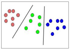
(a) Softmax Loss

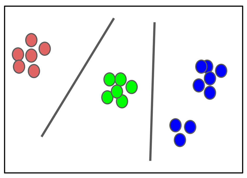
(b) Triplet Loss Regularizer

Figure 1: Softmax learns powerful representations with limited embedding regularization. Triplet loss promotes better embedding without an explicit number of class centers.

Embedding losses have been successfully applied in conjunction with softmax loss as regularizers. For example, center loss [42] was proposed for better face recognition efficiency. Magnet loss [29] generalizes the unimodality assumption of center loss. A recent triplet-center loss (TCL) [9] uses only a unimodal embedding but introduced a repelling force between class centers, i.e., inter-class margin maximization. All these methods assume a fixed number of class centers (embedding modes) for all classes.

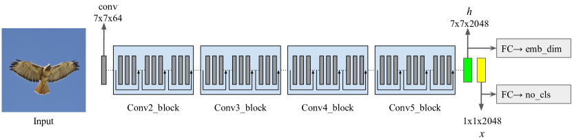
Figure 2: Our proposed two-head architecture builds on standard networks – ResNet used for visualization, $x_{input}=pool(h_{input})$. Besides computing classification logits, the pre-logits layer supports the embedding head. Softmax and triplet losses are applied to the classification logits and embedding features, respectively.

Unlike the aforementioned approaches, the standard triplet loss requires no explicit number of embedding modes. Thus, it avoids computing class centers while promoting intra-class compactness and inter-class margin maximization. Surprisingly, recent papers [42, 9] do not report the softmax+triplet loss quantitative evaluation. Assumptions about large training batch requirement [32] for faster convergence or high batch-processing complexity, to compute pairwise distance matrix, have hindered triplet loss’s adoption. Our experiments reassess these assumptions through multiple triplet loss sampling strategies.

To incorporate embedding losses, previous approaches employ loss-specific architectures. This custom setting is imperfect for the softmax baseline as it omits the pre-trained ImageNet weights. Through our proposed seamless integration into standard CNNs, we push our baselines’ limits. We introduce an embedding head similar to the classification head. Each head applies a single fully connected (FC) layer on the pre-logit convolutional layer features. Figure 2 shows our two head architecture where the pre-logit convolutional features support both softmax and triplet losses for classification and embedding respectively. This integration boosts classification performance while promoting better embedding.

We evaluate our approach on various classification domains. The first is a fine-grained visual recognition (FGVR) across five datasets. The second domain is an ego-motion action recognition task with high class imbalance. Large improvements (1-4%) are achieved in both domains. Evaluation on multiple architectures with the same hyper-parameters highlights our approach’s generality. The large batch size requirement represents a key challenge for triplet loss adoption; Schroff et al. [32] use a batch-size $b=1800$ and trained on a CPU cluster for 1,000 to 2,000 hours. In our experiments, we show that using a small batch size $b=32$ still improves performance. A further qualitative evaluation highlights beneficial qualities like nearest neighbor retrieval added to standard classification architectures. In summary, the key contributions of this paper are:

1. A two-head architecture proposal that uses triplet loss as a regularizer to boost standard architectures’ performance through promoting a better feature embedding.

2. A re-evaluation of the large batch size requirement and high computational cost assumptions for triplet loss,

3. Enable better nearest neighbor retrieval on standard classification architectures.

2 Related Work

Visual recognition deep networks employ softmax loss as follows

$$L_{\text{soft}}=-\sum_{i=1}^{b}{\log{\frac{{e}^{{W}_{{y}_{i}}^{T}{x}_{i}}}{\sum_{j=1}^{n}{{e}^{{W}_{{j}}^{T}{x}_{i}}}}}},$$ (1)

where $x_{i}\in R^{d}$ denotes the $i$th deep feature, belonging to the $y_{i}$th class. In standard architectures, $x_{i}$ is the pre-logit layer; the result of flattening the pooled convolutional features as shown in Figure 2. $W_{j}\in R^{d}$ denotes the $j$th column of the weights $W\in R^{d\times n}$ in the last fully connected layer. $b$ and $n$ are the batch size and the number of class respectively. The softmax loss only cares about separating samples from different class. It disregards properties like intra-class compactness and inter-class margin maximization. Embedding regularization is one way to tackle this limitation. Figure 3 depicts different embedding regularizers; all require an explicit number of embedding modes.

(a) Softmax Loss

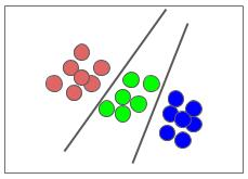
(b) Center Loss Regularizer

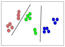
(c) Magnet Loss Regularizer

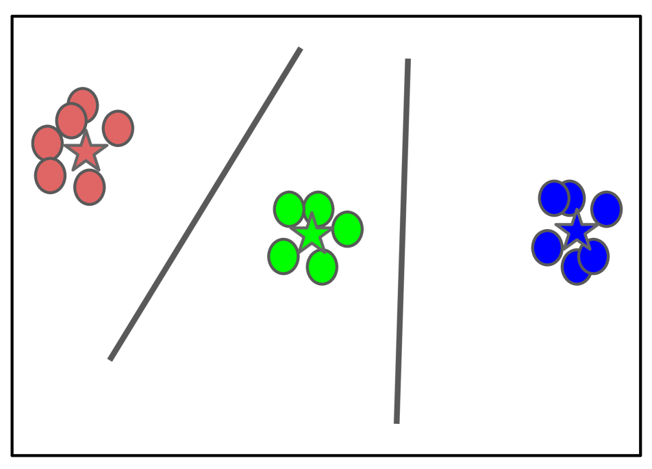
(d) Triplet Center Regularizer

Figure 3: Visualization of softmax and feature embedding regularizers. Softmax separates samples with neither class compactness nor margin maximization considerations. Center loss promotes unimodal compact class while magnet loss supports multi-modal embedding. Triplet center loss strives for unimodal, margin maximization and class compactness. The computed classes’ centers are depicted using a star symbol

2.1 Center Loss

Wen et al. [42] propose center loss to minimize intra-class variations. By maintaining a per class representative feature vector $c_{yi}\in R^{d}$, the novel loss term in equation 2 is proposed. The class centers are computed by averaging corresponding class features. They are updated after every training mini-batch. To avoid perturbations caused by noisy samples, a hyper-parameter $\alpha$ controls the learning rate of the centers, i.e., moving average.

$$L_{\text{cen}}=\frac{1}{2}\sum_{i=1}^{b}{{\parallel x_{i}-c_{yi}\parallel}_{2}^{2}}.$$ (2)

2.2 Magnet Loss

Rippel et al. [29] propose a center loss term supporting multi-modal embedding, dubbed magnet loss. It computes $K$ class representatives, i.e., K-clusters per class. Each sample is iteratively assigned to one of the K clusters and pushed towards its center. The magnet loss adaptively sculpts the representation space by identifying and enforcing intra-class variation and inter-class similarity. This is formulated as follows

$$\scalebox{0.95}[1.0]{$L_{M}=\frac{1}{N}\sum_{i=1}^{N}{-\log{\frac{\exp({\begin{matrix}\frac{-1}{2{\sigma}^{2}}{\parallel{x}_{i}^{k}-{\mu}_{k}^{c}\parallel}_{2}^{2}-\alpha\end{matrix}})}{\sum_{c\neq C({x}_{i}^{k})}{\sum_{k=1}^{K}{\exp({\begin{matrix}\frac{-1}{2{\sigma}^{2}}{\parallel{x}_{i}^{k}-{\mu}_{k}^{c}\parallel}_{2}^{2}-\alpha\end{matrix}})}}}}}$},$$ (3)

where $N$ and $K$ are the number of samples and clusters per class respectively. $x_{i}^{k}\in R^{d}$ denotes the $i$th deep feature, belonging to cluster $k$ in the $y_{i}$th class, $\mu_{k}^{c}\in R^{d}$ is the $k$th cluster center belonging to class $c$. Finally ${\sigma}^{2}=\frac{1}{N-1}\sum{{\parallel{x}_{i}^{k}-{\mu}_{k}^{c}\parallel}_{2}^{2}}$ is the variance of all samples from their respective centers. One criticism of magnet loss is the complexity overhead to maintain multiple clusters per class and their assigned samples. Moreover, the constant number of clusters per-class disputes with imbalanced data distributions.

2.3 Triplet Center Loss

While promoting class compactness, the center loss depends on the softmax loss supervision signal to push different classes apart. The learned features optimized with the softmax loss supervision signal are not discriminative enough, i.e., no explicit repelling force pushes different classes apart. Inter-class clusters can overlap due to missing an explicit inter-class repelling incentive. He et al. [9] propose triplet center loss (TCL) to avoid this limitation. By maintaining a per class center $c_{yi}\in R^{d}$ similar to [42], TCL is formulated as follows

$$L_{\text{tcl}}=\sum_{i=1}^{b}{{\left[{(D({x}_{i},{c}_{yi})-\min_{j\neq i}{D({x}_{i},{c}_{yj})}+m)}\right]}_{+}},$$ (4)

where $m$ is a separating margin, ${\left[.\right]}_{+}=max(0,.)$ and $D(.)$ represents the squared Euclidean distance function.

Triplet loss is a well-established surrogate for TCL. It achieves the intra and inter-class embedding objectives without computing class centers. Yet, it is largely avoided for its computational complexity and large training batch requirement assumptions. In the experiment section, we address these concerns and evaluate the utility of triplet loss as a regularizer. Our approach is evaluated on the challenging FGVR task where intra-class overwhelm inter-class variations. Further evaluation on the Honda driving dataset (HDD) demonstrates our approach’s competence on an imbalanced video dataset. Triplet loss regularization not only lead to higher classification accuracy but also enables better feature embedding.

3 The Triplet Loss Regularizer

The next subsection introduces triplet loss [32] as a softmax loss regularizer. Then, we explain our standard architectural extension to integrate an embedding loss.

3.1 Triplet Loss

Triplet loss [32] has been successfully applied in face recognition [32, 31] and person re-identification [3, 35, 30]. In both domains, it is used as a feature embedding tool to measure similarity between objects and provide a metric for clustering. In this work, we utilize triplet loss as a classification regularizer. It is more efficient than contrastive loss [7, 20], and less computationally expensive than quadruplet [13, 2] and quintuplet [12] losses. While the pre-logits layer learns better representations for classification using the softmax loss, triplet loss promotes a better feature embedding. Equation 5 shows the triplet loss formulation

$$L_{\text{tri}}=\frac{1}{b}\sum_{i=1}^{b}{{\left[{(D(a_{i},p_{i})-{D(a_{i},n_{i})}+m)}\right]}_{+}},$$ (5)

where an anchor image’s embedding $a$ of a specific class is pushed closer to a positive image’s embedding $p$ from the same class than it is to a negative image’s embedding $n$ of a different class. Equation 6 is our loss function with a balancing hyper-parameter $\lambda$.

$$L=L_{\text{soft}}+\lambda L_{\text{tri}}.$$ (6)

Sampling: Triplet loss performance is dependent on its sampling strategy. We evaluate both the hard [10] and semi-hard [32] sampling strategies. In semi-hard negative sampling, instead of picking the hardest positive-negative samples, all anchor-positive pairs and their corresponding semi-hard negatives are considered. Semi-hard negatives satisfy equation 7. They are further away from the anchor than the positive exemplar, yet within the banned margin $m$.

$$D(a,p)<{D(a,n)}<D(a,p)+m.$$ (7)

Figure 4 shows a triplet loss tuple and highlights the different types of negative exemplars: easy ($n_{2}$), semi-hard ($n_{1}$) and hard ($n_{3}$) negatives. An easy negative satisfies the margin constraint and suffers a zero loss. Unlike hard-sampling, semi-hard sampling supports a multi-modal embedding. Hard sampling picks the farthest positive and nearest negative without any consideration for the margin. In contrast, Figures 5 illustrates how semi-hard sampling ignores hard negatives. Two classes, red and green, are embedded into one and two clusters respectively. A hard sampling strategy pulls the farthest positive from one cluster to the anchor in the other cluster, i.e. promotes a merge. The semi-hard sampling strategy omits this tuple because the negative sample is nearer than the positive.

The existence of a semi-hard negative is not guaranteed in small batches, especially near convergence. Thus, we prioritize negative exemplars as illustrated in Figure 4. First priority is given to semi-hard ($n_{1}$), then easy ($n_{2}$) and finally hard negatives ($n_{3}$).

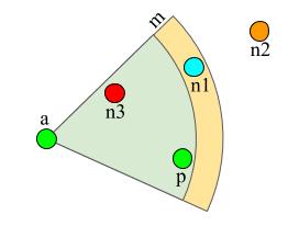
Figure 4: Triplet loss tuple (anchor, positive, negative) and margin $m$. Hard, semi-hard and easy negatives highlighted in red, cyan and orange, respectively.

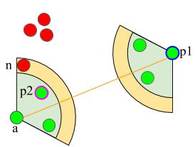
Figure 5: Hard sampling promotes unimodal embedding by picking the farthest positive and nearest negative $(a,p1,n)$. Semi-hard sampling picks $(a,p2,n)$ and avoids any tuple $(a,p,n)$ where $n$ lies between $a$ and $p$.

3.2 Two-Head Architecture

Standard convolutional architectures, with ImageNet [4] weights, are employed in various applications for their powerful representation. We seek to leverage pre-trained standard networks for their advantages in tasks like fine-grained visual recognition [22, 18, 17]. This key integration promotes the generality of our approach and distances our work from  [42, 9, 36] which use custom architectures. Through experiments, we demonstrate how triplet loss achieves superior classification efficiency compared to center loss.

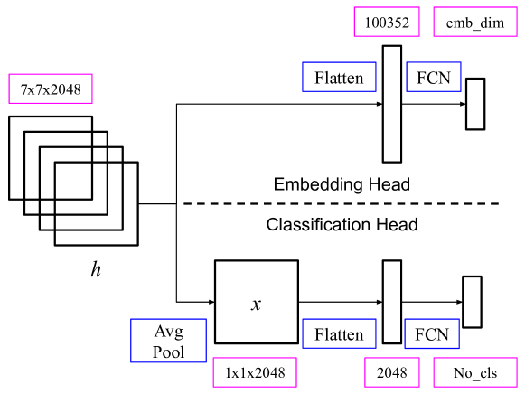
Figure 6: Our proposed two-head architecture. The last convolutional feature map ($h$) supports both embedding and classification heads. Operations and dimensions are highlighted with blue and pink colors, respectively. ResNet-50 dimensions used for illustration.

Unlike VGG [34], recent architectures [8, 39, 14] employ a convolutional layer before the classification head. To generate logits, the classification head pools the convolutional layer features, flatten them, then utilize a customizable fully connected layer to support various numbers of classes. Similarly, we integrate triplet loss to regularize embedding as shown in Figure 6. Before pooling, we flatten the convolutional layer features then apply another fully connected layer $W_{\text{emb}}$ to generate embeddings as illustrated in equation 11.

Logits $$=W_{\text{logits}}*\text{flatten}(x)$$ (8)

Embedding $$=W_{\text{emb}}*\text{flatten}(h),$$ (9)

where $x=\text{pool}(h)$. Orderless pooling, like averaging, disregard spatial information. Thus, a fully connected layer $W_{\text{emb}}$ applied on $h$ has a better representation power. The final embedding is normalized to the unit-circle and the square Euclidean distance metric is employed. During inference, the two-head architecture enables both classification and retrieval with negligible overhead.

4 Experiments

4.1 Evaluation on FGVR

	Flowers-102 [26]	Aircrafts [25]	NABirds [41]	Stanford Cars [19]	Stanford Dogs [15]
Num Classes	102	100	550	196	120
Avg samples Per Class	10	100	43.5	41.55	100
Train Size	1020	3334	23929	8144	12000
Val Size	1020	3333	N/A	N/A	N/A
Test Size	6149	3333	24633	8041	8580
Total Size	8189	10000	48562	16185	20580

Table 1: Statistics of five FGVR datasets and their corresponding train, validation and test splits.

Datasets: We evaluate our approach on five FGVR datasets. These datasets comprise both make/model classification and wildlife species. The Aircrafts dataset contains 10,000 images of aircraft spanning 100 aircraft-models. The finer level differences between models makes visual recognition challenging. The NABirds dataset contains 48,562 images across 550 visual categories of North American birds. The Flower-102 dataset contains 8189 images across 102 classes. The Stanford Cars dataset contains 16185 images across 196 car classes that represent variations in car make, model, and year. Finally, the Stanford Dogs dataset has 20,580 images across 120 breeds of dogs. These datasets provide challenges in terms of large intra-class but small inter-class variations. Table 1 summarizes the datasets’ size, number of classes and splits.

Baselines: We evaluate our approach against two baselines: (1) Single head softmax; (2) Two-head leveraging center loss [42] with it’s proposed hyper-parameters $\lambda=0.003$ and $\alpha=0.5$. We found Magnet loss [29] implementation computationally expensive. It applies k-means to cluster all training samples after each epoch, i.e., $O(N^{2})$ where $N$ is the train split size. For triplet loss, both hard [10] and semi-hard [32] sampling variants are evaluated. By default, our hyper-parameter $\lambda=1$ and embedding normalized to the unit circle with dimensionality $d_{\text{emb}}=256$. With triplet hard sampling, a soft margin between classes is imposed by the softplus function $\ln(1+\exp(\mathbin{\vbox{\hbox{\scalebox{0.75}{$\bullet$}}}}))$. It is similar to the hinge function $\max(\mathbin{\vbox{\hbox{\scalebox{0.75}{$\bullet$}}}},0)$ but it decays exponentially instead of a hard cut-off. With triplet semi-hard sampling, we employ the hard margin $m=0.2$ as proposed by [32]

All experiments are conducted on Titan Xp 12GB GPU with batch-size $b=32$. All networks are initialized with ImageNet weights, and then fine-tuned. Momentum optimizer is utilized with momentum $0.9$ and a polynomial decaying learning rate $lr=0.01$. We quantitatively evaluate our approach on three architectures: (1) ResNet-50 [8] and (2) DenseNet-161 [14] both trained for 40K iterations, and (3) Inception-V4 [37] trained for 80K iterations. While early stopping is a valid regularization form to avoid a fixed number of training iteration, not all datasets provide a validation split as illustrated in table 1. The chosen number of training iterations achieve comparable results with recent FGVR softmax baselines [21, 18, 5].

To evaluate our approach, our training batches contain both positive and negative samples. We follow the batch construction procedure proposed by Hermans et al. [10]. A class is uniformly sampled then $K=4$ sample images, with resolution $224\times 224$, are randomly drawn. Training images are augmented online with random cropping and horizontal flipping. This process iterates until a batch is complete. Table 2 presents our fine-tuning quantitative evaluation on the five datasets. Our two-head architecture with hard triplet loss achieves large steady (1-4%) improvement on ResNet-50. Similar trend appears with Inception-V4 but suffers an interesting fluctuation between hard and semi-hard triplet loss. Section 4.3 reflects on this phenomena through a quantitative embedding analysis. Vanilla DenseNet-161 achieves comparable state-of-the-art results on all FGVR datasets, yet triplet loss regularizer maintains a steady trend of performance improvement.

Center loss achieves an inferior classification performance especially on the Dogs dataset – a lag $\approx 4\%$ behind vanilla softmax on Inception-V4 and DenseNet-161. The single mode embedding assumption is valid for face recognition [42] and vehicle re-identification [23] because different images for the same identify belong to a single cluster. However, when working with categories of high intra-class variations, this assumption degenerate the feature embedding quality. Our feature embedding evaluation (Sec  4.3) highlights the consequence of using a single mode/cluster, for general classification problems, in terms of feature embedding instability or collapse.

Our simple but vital integration into standard architectures distance our approach from similar softmax+clustering formulations. In addition, all recent convolutional architectures share similar ending structure; the last convolutional layer is followed by an average pooling, and then a single fully connected layer. Thus, apart from the studied architectures, our secondary embedding head proposal can be applied to other architectures, e.g., MobileNet [11].

Database	Cars	Flowers	Dogs	Aircrafts	Birds
ResNet-50
Softmax	85.85	85.68	69.76	83.22	64.23
Two-Head (Center)	88.23	85.00	70.45	84.48	65.5
Two-Head (Semi)	88.22	85.52	70.69	85.08	65.20
Two-Head (Hard)	89.44	86.61	72.70	87.33	66.19
Inception-V4
Softmax	88.42	88.22	77.20	86.76	74.90
Two-Head (Center)	89.50	88.35	70.83	87.78	76.86
Two-Head (Semi)	89.72	88.69	77.71	88.59	76.99
Two-Head (Hard)	89.06	90.66	75.97	89.04	76.57
DenseNet-161
Softmax	91.64	92.56	81.58	89.13	78.69
Two-Head (Center)	89.08	92.58	77.02	89.97	79.05
Two-Head (Semi)	92.36	93.65	80.89	89.64	79.57
Two-Head (Hard)	92.41	93.25	81.16	89.34	79.47

Table 2: Quantitative evaluation on the five FGVR datasets using ResNet-50, Inception-V4, and DenseNet-161.

4.2 Task Generalization

For further evaluation, we leverage the Honda Research Institute Driving Dataset (HDD) [28] for action recognition. HDD is an ego-motion video dataset for driver behavior understanding and causal reasoning. It contains 10,833 events spanning eleven event classes. Moreover, the HDD event class distribution is long-tailed which poses an imbalance data challenge. Figure 7 shows the eleven event classes with their distributions. To reduce video frames’ redundancy, three frames are sampled per second, and events shorter than 2 seconds are omitted.

Figure 7: Honda driving dataset long tail class distribution

Figure 8: Stack of difference motion encoding. Instead of six frames, three are used for visualization purpose. The first row shows a stack of two difference frames constructed by subtracting consecutive pairs of grayscale frames in the second row. These images are best viewed in color/screen.

To leverage standard architecture for action recognition, stack of difference (SOD) motion encoding proposed by Fernando et al. [6] is adopted. While better motion encoding like optical-flow exists, the SOD is utilized for its simplicity and ability to achieve competitive results [6, 40]. Given a sequence of frames representing an event, six consecutive frames spanning 2 seconds are randomly sampled. They are converted to grayscale, and then every consecutive pair is subtracted to create a stack of difference $\in Z^{W\times H\times 5}$ as depicted in Figure 8. Standard architectures are easily adapted to this input representation by treating the SOD input as a five-channel image instead of three.

Unlike FGVR input $\in[0,255]$, SOD $\in[-255,255]$. Thus, a ResNet-50 [8] architecture initialized with random weights is employed. It is trained for 10K iterations with $\lambda=1$ and a polynomial decaying learning rate $lr=0.01$. Batch sizes 33 and 63 are used to compare the vanilla softmax against our approach. To highlight performance on minority classes, both micro and macro average accuracies are reported in Table 3. Macro-average computes the metric for each class independently before taking the average. Micro-average is the traditional mean for all samples. Macro-average treats all classes equally while micro-averaging favors majority classes. Table 4 highlights the efficiency of our approach on minority classes.

	Micro Acc	Macro Acc
Softmax ($b=33$)	84.43	47.66
Two-head (Semi) ($b=33$)	84.93	53.70
Softmax ($b=63$)	84.45	46.53
Two-head (Semi) ($b=63$)	84.85	54.08

Table 3: Action recognition quantitative evaluation on the Honda dataset. $b$ indicates the batch-size used. Macro average accuracy highlights performance on minority classes.

	Softmax	Two-Head	Softmax	Two-Head
Event	Batch-size 33		Batch-size 63
Background	96.28	95.29	97.32	96.28
Intersection Passing	74.61	75.86	74.26	74.68
Left Turn	85.49	84.87	85.18	86.11
Right Turn	88.47	87.22	86.91	86.60
Left Lane Change	59.40	66.33	55.44	62.37
Right Lane Change	44.79	61.45	40.62	51.04
Cross-walk Passing	18.18	18.18	12.12	12.12
U-Turn	0.00	11.76	0.00	23.52
Left Lane Branch	53.84	64.10	41.02	64.10
Right Lane Branch	0.00	6.24	12.49	18.74
Merge	3.22	19.35	6.45	19.35
Macro Accuracy	47.66	53.70	46.53	54.08

Table 4: Detailed evaluation on the Honda driving dataset. Our two-head architecture using semi-hard triplet loss achieves better performance on minority classes.

4.3 Retrieval Evaluation on FGVR

In the two-head architecture, the secondary embedding head brings values like an enhanced feature embedding, nearest neighbor retrieval and interpretability. Following Song et al. [27], we evaluate the quality of feature embedding using Recall@K metric on the test split. We also leverage the Normalized Mutual Info (NMI) score to evaluate the quality of cluster alignments. $\text{NMI}=\frac{I(\Omega,C)}{\sqrt{H(\Omega)H(C)}},$ where $\Omega=\{\omega_{1},..,\omega_{n}\}$ is the ground-truth clustering while $C=\{c_{1},...c_{n}\}$ is a clustering assignment for the learned embedding. $I(\mathbin{\vbox{\hbox{\scalebox{0.5}{$\bullet$}}}},\mathbin{\vbox{\hbox{\scalebox{0.5}{$\bullet$}}}})$ and $H(\mathbin{\vbox{\hbox{\scalebox{0.5}{$\bullet$}}}})$ denotes mutual information and entropy respectively. We use K-means to compute $C$.

		NMI	R@1	R@4	R@8	R@16
Car - ResNet	CNTR	0.549	67.73	75.36	81.91	87.28
	SEMI	0.879	89.45	93.14	95.24	96.62
	HARD	0.900	91.95	94.22	95.70	96.78
Flowers - ResNet	CNTR	0.723	74.53	86.78	90.94	94.06
	SEMI	0.822	87.56	94.29	96.39	97.89
	HARD	0.856	90.40	94.00	94.84	95.64
Dogs - ResNet	CNTR	0.419	30.41	40.69	63.96	75.14
	SEMI	0.708	60.70	79.55	85.84	90.15
	HARD	0.740	64.01	81.60	86.41	89.97
Aircrafts - ResNet	CNTR	0.645	64.36	80.32	85.57	89.41
	SEMI	0.846	82.15	90.01	92.38	94.45
	HARD	0.879	85.84	91.63	92.89	93.94
NABirds - ResNet	CNTR	0.517	32.16	50.89	60.03	68.70
	SEMI	0.749	56.30	76.08	82.99	88.30
	HARD	0.769	59.09	77.35	83.49	88.12
Cars - Inc-V4	CNTR	0.120	2.98	5.96	8.84	13.87
	SEMI	0.880	85.45	93.56	95.66	97.15
	HARD	0.652	46.97	71.14	80.87	87.90
Flowers - Inc-V4	CNTR	0.183	9.01	11.97	13.82	16.13
	SEMI	0.828	88.70	94.70	96.47	97.89
	HARD	0.885	93.66	96.13	96.96	97.59
Dogs - Inc-V4	CNTR	0.726	65.47	76.62	79.01	81.04
	SEMI	0.760	68.48	85.10	90.26	93.83
	HARD	0.458	19.52	41.41	55.63	70.63
Aircrafts - Inc-V4	CNTR	0.333	27.21	36.75	42.81	49.62
	SEMI	0.872	86.53	92.35	93.88	95.08
	HARD	0.887	87.79	92.47	93.67	94.42
NABirds - Inc-V4	CNTR	0.209	3.77	6.26	8.29	11.50
	SEMI	0.808	67.30	83.81	88.96	92.79
	HARD	0.503	15.92	31.84	42.66	54.64
Cars - Dense	CNTR	0.914	88.93	93.97	95.01	95.65
	SEMI	0.905	88.77	95.72	97.08	98.30
	HARD	0.913	89.40	95.57	96.99	98.15
Flowers - Dense	CNTR	0.910	95.23	97.19	97.61	98.13
	SEMI	0.869	94.52	97.90	98.68	99.14
	HARD	0.898	87.73	91.87	92.32	92.65
Dogs - Dense	CNTR	0.795	72.03	84.11	86.55	88.39
	SEMI	0.802	73.33	88.24	92.21	95.02
	HARD	0.807	73.99	88.66	92.44	94.99
Aircrafts - Dense	CNTR	0.898	87.73	91.87	92.32	92.65
	SEMI	0.883	86.98	93.49	95.11	96.28
	HARD	0.889	87.82	94.27	95.38	96.07
NABirds - Dense	CNTR	0.847	76.90	85.37	88.03	90.57
	SEMI	0.829	72.09	86.90	91.24	94.35
	HARD	0.829	72.02	87.11	91.61	94.70

Table 5: Detailed feature embedding quantitative analysis across the five datasets using ResNet-50, Inception-V4 and DenseNet-161. Triplet with hard mining achieves superior embedding with ResNet-50 trained for 40K iterations. Semi-hard triplet is competitive and stable with Inception-V4 trained for 80K iterations. Center loss learns an inferior embedding while suffering the highest instability.

Table 5 presents a detailed feature embedding quantitative analysis. Triplet loss with hard-mining consistently learns the best embedding on ResNet-50. However, semi-hard sampling, on Inception-V4 and DenseNet, is stabler. Despite having an explicit rebelling force pushing negative samples away from their anchors, hard triplet mining can in practice lead to bad local minima (as can be seen in inception-V4). It can result in a collapsed mode $(\emph{i.e}.\hbox{},f(x)=0)$ [32]. Center loss suffers the same model collapse problem. It is a more vulnerable variant of hard-triplet loss, i.e., missing the repelling force. It learns an inferior embedding while suffering the highest instability. It often degenerates with Inception-V4. These conclusions follow Schroff et al. [32] semi-hard mining findings.

Table 6 compares classification and retrieval performance quantitatively. The reported classification accuracy provides an upper bound for retrieval. Retrieval and classification top 1 accuracies are comparable. Recall@4 is superior to the classification top 1 on all datasets. Figure 9 presents a qualitative retrieval evaluation across center loss, triplet semi-hard, and triplet hard regularizers.

	Cars	Flowers-102	Dogs	Aircrafts	NABirds
	ResNet-50
Classification Top 1	89.44	86.61	72.70	87.33	66.19
Retrieval Top 1	91.95	90.40	64.01	85.84	59.09
Retrieval Top 4	94.22	94.00	81.60	91.63	77.35
	Inception-V4
Classification Top 1	89.72	90.66	77.71	89.04	76.99
Retrieval Top 1	85.45	93.66	68.48	87.79	67.30
Retrieval Top 4	93.56	96.13	85.10	92.47	83.81
	DenseNet-161
Classification Top 1	92.36	93.65	81.58	89.97	76.57
Retrieval Top 1	89.40	95.23	73.99	87.82	76.90
Retrieval Top 4	95.72	97.90	88.66	94.27	87.11

Table 6: Comparative quantitative evaluation between retrieval and classification as an upper bound. Both retrieval and classification accuracies are comparable. Retrieval top 4 is superior to classification top 1.

Query $\downarrow$				Query $\downarrow$				Query $\downarrow$

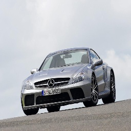
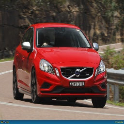
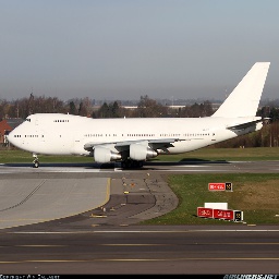
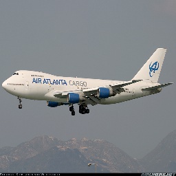
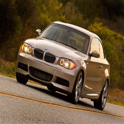
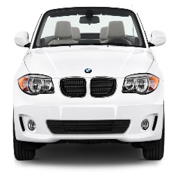
Figure 9: Retrieval qualitative evaluation on three FGVR datasets: Flowers-102, Aircrafts and Cars. Given a query image, the three nearest neighbors are depicted. The three consecutive rows show search results using center loss, semi-hard and hard triplet regularizers. Green and red outlines denote match and mismatch between the query and it’s result respectively.

It is challenging, for the current classification architectures, to interpret a test image misclassification. By learning image embedding through a secondary head, it becomes trivial to investigate an image’s test and train splits neighborhood. Figure 10 shows nine (three images per odd column) misclassified test images and their corresponding nearest neighbor from the train split. The resembles between a misclassified test image and a particular training image can reveal corner cases omitted while collecting the data. One interesting statistic is that 79.34% of misclassified predictions, from Flowers-102 test split, match the label of their nearest training neighbor. This emphasizes the classification complexity level of FGVR.

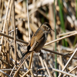
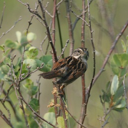
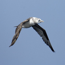
Figure 10: Qualitative misclassification interpretation. The odd columns show a misclassified test image while the even columns show the nearest neighbor from the training split.

4.4 Ablation Analysis

Hyper-Parameter Stability: Our approach has two hyper-parameters: $\lambda$ and the embedding dimensionality $d_{\text{emb}}$. $\lambda$ is tuned on the Flowers-102 dataset through the validation split. All hyper-parameter tuning experiments are executed for 2000 iterations. Figure 11 highlights $\lambda$ stability within $[0.1,2]$. A larger $\lambda$ making triplet loss dominant is discouraged. Intuitively, further hyper-parameters tuning can achieves better performance.

Figure 11: Hyper-parameter $\lambda$ tuning on the Flowers-102 dataset.

Two-Head Time Complexity: The computational cost of the embedding head is negligible. Both sampling and backpropagation are implemented on GPU. Training time increases by $1\%,3\%,$ and $2\%$ for semi-hard, hard and center losses on Titan XP GPU, respectively. Figure 12 shows a time complexity analysis in terms of batch processing time (secs). Please note that triplet loss approaches retain from computing classes centers or enforcing a specific number of modes.

Figure 12: Two-head time complexity analysis on ResNet-50, Inception-V4 and DenseNet-161 using Flowers-102 dataset.

4.5 Discussion

Our experiments demonstrate how a two-head architecture with triplet loss outperforms a vanilla single-head softmax network. Triplet loss attains the center loss, triplet center loss and magnet loss objectives without enforcing explicit class representatives. It promotes both intra-class compactness and inter-class margin maximization. Semi-hard triplet loss relaxes the unimodal embedding constraint while maintaining stabler learning curve. Hard triplet loss achieves larger improvement margins but can suffer model collapse. Triplet loss effectively regularizes softmax and promote better feature embedding.

The two-head architecture with triplet loss is the main scope of this paper. Investigating other recent ranking losses, e.g. Margin loss [43], and comparing their benefits to softmax remains an open question.

5 Conclusion

We propose a seamless integration of triplet loss as an embedding regularizer into standard classification architectures. The regularizer competence is illustrated on multiple datasets, architectures and recognition tasks. Triplet loss, without the large batch requirement, boosts standard architectures’ performance. With minimal hyper-parameter tuning and a single fully connected layer on top of pretrained standard architectures, we promote generality to novel domains. Promising results are achieved on an imbalanced dataset. We incur a minimal computational overhead during training, but raise classification model efficiency and interpretability. Our architectural extension enables both retrieval and classification tasks during inference.

6 Supplementary Material

The next subsections provide more details about our architecture and training procedure’s technicalities. Further quantitative evaluations on fine-grained visual recognition (FGVR) are presented. Finally, we demonstrate the training procedure for the Honda Research Institute Driving Dataset.

6.1 Fine-Grained Visual Recognition

Figure 2 in the main paper presents our two-head architecture. The pre-logit layer $x$ supports the softmax loss. Similarly, triplet loss utilizes $h$, where $x=pool(h)$. The network outputs, both logits and embedding, are formulated as follows.

logits $$=W_{\text{logits}}*\text{flat}(x)$$ (10)

embedding $$=W_{\text{emb}}*\text{flat}(h).$$ (11)

Orderless pooling, like averaging, reduces $h$ dimensionality but loses spatial information. For example, in DenseNet161, $h\in R^{7\times 7\times 2208}$ while $x\in R^{1\times 1\times 2208}$. Thus, $W_{\text{emb}}$ employs $h$, instead of $x$, to improve feature embedding. Figure S1 illustrates how $h$ provides a finer control level while learning $W_{\text{emb}}$.

Figure S2 shows a t-SNE visualization for Flowers-102 embedding using 50 random classes, 20 samples per class. In the main paper, the inferior performance of triplet loss with hard-mining is associated with convergence to bad local minima, i.e., a collapsed model $(\emph{i.e}.\hbox{}f(x)=0)$ [32]. To examine such assumption, we train a DenseNet for 400K iterations on Stanford Dogs. This large number of iterations increases the chances of a model collapse. Figure S3 presents the performance on the test split after every 50K iterations. Triplet loss with hard-mining is evaluated with both soft and hard margin. Soft margin applies the softplus function $\ln(1+\exp(\mathbin{\vbox{\hbox{\scalebox{0.75}{$\bullet$}}}}))$ while hard margin uses a fixed margin $m=0.2$. The triplet loss with hard-mining deteriorates with soft margin when trained for a large number of iterations. Hard-mining with hard margin is more robust. We found similar behavior on other datasets like Stanford Cars and Aircrafts datasets.

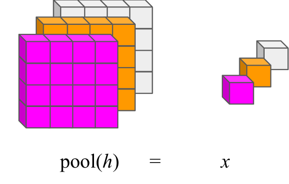
Figure S1: Orderless pooling reduces dimensionality but loses features spatial information.

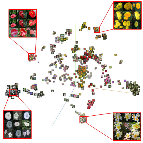
Figure S2: t-SNE visualization for Flowers-102 embedding using 50 random classes, 20 samples per class. Best viewed in color.

Figure S3: Model collapse study by training DenseNet161 for 400K iterations. Triplet loss with hard-mining evaluated with soft and hard margins.

Table 5 in the main paper presents a quantitative analysis for the feature embedding learned by the second head in our proposed architecture. Similarly, Table S1 presents feature embedding quantitative analysis using the architecture penultimate layer, i.e., layer $x$ (Figure 2 in the main paper). This layer is present in both our proposed two-head and single-head (vanilla softmax) architecture. Similar to Table 5, the triplet loss embedding is superior to the softmax embedding. Triplet loss with hard-mining achieves the best results on ResNet-50 but degrades on Inception-V4 trained for 80K iterations. Center loss achieves good results with DenseNet161 on NABirds but generally fluctuates and suffers with Inception-V4. Triplet loss with semi-hard margin achieves sub-optimal embedding but maintains the highest stability compared to center and hard-mining approaches.

Figure S4 graphically summarizes Table S1. It provides a comparative embedding evaluation between the single-head softmax verses the two-head with semi-hard triplet loss using recall@1 metric. Triplet loss improvements, over the softmax model, are reported as ($\triangle$). The Flowers-102 dataset has the smallest training split with 1020 images only. With this limited data, the head-two architecture achieves marginal improvement if any.

Table S2 compares our proposed two-head architecture, using DenseNet161, with state-of-the-art approaches on the five FGVR datasets. Our two-head architecture with the semi-hard triplet loss regularizer achieves competitive results.

		NMI	R@1	R@4	R@8	R@16
Cars - ResNet	Vanilla	0.791	77.88	91.17	94.65	96.9
	CNTR	0.756	77.98	91.12	94.58	96.78
	SEMI	0.823	81.41	92.79	95.91	97.74
	HARD	0.853	85.31	94.30	96.82	98.07
Flowers - ResNet	Vanilla	0.800	88.76	95.51	97.27	98.49
	CNTR	0.807	88.79	95.58	97.32	98.49
	SEMI	0.818	89.48	95.82	97.37	98.37
	HARD	0.742	90.78	95.56	96.93	97.98
Dogs - ResNet	Vanilla	0.587	51.62	74.22	83.02	89.76
	CNTR	0.526	48.74	71.90	80.92	87.81
	SEMI	0.621	54.18	76.39	84.50	91.10
	HARD	0.684	60.37	80.34	87.33	92.26
Aircrafts - ResNet	Vanilla	0.756	73.42	87.88	92.26	94.90
	CNTR	0.677	70.84	85.84	90.79	93.91
	SEMI	0.792	77.26	89.65	93.07	95.29
	HARD	0.829	84.01	91.63	94.21	95.65
NABirds - ResNet	Vanilla	0.669	50.70	71.20	79.48	85.80
	CNTR	0.623	47.40	68.18	76.56	83.33
	SEMI	0.657	50.05	70.83	78.84	85.52
	HARD	0.723	55.85	75.81	83.26	88.67
Cars - Inc-V4	Vanilla	0.660	72.47	86.77	90.55	93.55
	CNTR	0.496	61.55	79.09	85.09	89.69
	SEMI	0.788	81.46	92.14	94.64	96.37
	HARD	0.566	63.70	82.04	87.54	91.42
Flowers - Inc-V4	Vanilla	0.778	90.54	96.21	97.63	98.70
	CNTR	0.707	85.62	93.74	95.95	97.56
	SEMI	0.801	89.58	95.23	96.91	97.84
	HARD	0.731	92.68	96.21	97.27	98.32
Dogs - Inc-V4	Vanilla	0.421	41.11	62.97	72.59	81.13
	CNTR	0.453	57.13	68.32	72.35	76.90
	SEMI	0.609	55.03	76.50	84.44	90.23
	HARD	0.330	33.89	54.28	65.06	74.98
Aircrafts - Inc-V4	Vanilla	0.680	69.79	85.18	89.23	91.93
	CNTR	0.546	61.60	79.75	85.33	89.53
	SEMI	0.751	78.13	89.20	91.78	94.27
	HARD	0.831	86.26	91.87	93.49	94.72
NABirds - Inc-V4	Vanilla	0.546	41.03	60.11	68.88	76.71
	CNTR	0.438	24.30	40.43	49.38	58.78
	SEMI	0.638	52.42	72.38	79.57	85.60
	HARD	0.433	23.68	38.95	47.48	57.10
Cars - Dense	Vanilla	0.813	85.08	94.49	96.84	98.22
	CNTR	0.787	87.39	93.17	94.64	95.97
	SEMI	0.875	88.57	96.08	97.66	98.71
	HARD	0.892	89.44	96.38	97.86	98.76
Flowers - Dense	Vanilla	0.838	95.28	98.23	98.94	99.38
	CNTR	0.812	95.87	98.16	98.75	99.22
	SEMI	0.864	95.40	98.39	99.09	99.46
	HARD	0.865	95.79	98.50	99.14	99.50
Dogs - Dense	Vanilla	0.544	57.06	78.72	85.98	91.84
	CNTR	0.720	70.96	84.00	88.19	91.96
	SEMI	0.728	68.55	87.04	92.18	95.83
	HARD	0.756	70.63	87.80	92.95	96.22
Aircrafts - Dense	Vanilla	0.768	79.06	91.66	94.66	96.49
	CNTR	0.792	86.20	91.63	93.16	94.48
	SEMI	0.853	84.49	94.15	95.68	96.97
	HARD	0.856	85.51	93.70	95.83	96.94
NABirds - Dense	Vanilla	0.606	53.91	73.08	80.70	86.44
	CNTR	0.818	75.28	86.88	90.85	93.69
	SEMI	0.677	61.82	80.70	87.07	91.62
	HARD	0.674	61.64	80.21	86.77	91.37

Table S1: Detailed feature embedding quantitative analysis across the five datasets using ResNet-50, Inception-V4 and DenseNet-161 architectures’ penultimate layer $x$. Triplet with hard mining achieves superior embedding with ResNet-50 trained for 40K iterations. Semi-hard triplet is competitive and stable with Inception-V4 trained for 80K iterations. Center loss suffers a high instability.

Figure S4: Comparative embedding evaluation between single-head softmax and two-head with semi-hard triplet loss using the penultimate layer in ResNet-50, Inception-V4 and DenseNet161 respectively. Triplet loss semi-hard improvements over the softmax model are reported as ($\triangle$).

Flowers-102

Method	Acc
Det.+Seg. [1]	80.66
Overfeat [33]	86.80
Softmax	92.56
Two-Head (Semi)	93.65

Aircrafts

Method	Acc
LRBP  [16]	87.30
Liu et al. [21]	88.50
Softmax	89.13
Two-Head (Semi)	89.64

NABirds

Method	Acc
Branson et al. [44]	35.70
Van et al. [18]	75.00
Softmax	78.69
Two-Head (Semi)	79.57

Cars

Method	Acc
Liu et al. [24]	86.80
Liu et al. [21]	92.00
Softmax	91.64
Two-Head (Semi)	92.36

Dogs

Method	Acc
Zhang et al. [44]	80.43
Krause et al. [18]	80.60
Softmax	81.58
Two-Head (Semi)	80.89

Table S2: Quantitative evaluation on the five FGVR datasets using DenseNet161. Our two-head architecture with semi-hard triplet loss regularizer compares favorably with state-of-the-art results.

6.2 Autonomous Car Driving

The Honda Research Institute Driving Dataset (HDD) contains 137 sessions $S$. Each session $S_{i}$ represents a navigation task performed by a driver. $S$ is divided into 93, 5, and 36 sessions for training, validation and testing splits respectively. Three sessions are removed for missing annotations. HDD has four annotation layers to study the drivers’ actions: (1) Goal-oriented, (2) stimulus-driven, (3) cause and (4) attention. The Goal-oriented layer, utilized in our experiments , defines drivers’ actions to reach their destinations, e.g., left-turn and intersection passing. Ramanishka et al. [28] provides further details for the other three annotation layers.

Triplet loss mini-batches require both positive and negative samples. The FGVR datasets have uniform class distribution. Thus, training batches’ construction is straight-forward by sampling random classes and their corresponding images as outlined in the main paper. On the other hand, HDD suffers class imbalance. A different batch construction procedure is required.

Algorithm 1 outlines our training procedure. First, $N_{B}$ mini-batches are constructed, each containing $b$ random actions. The batches’ embeddings are computed using $N_{B}$ feed forward passes. The $2D$ matrix $D_{\phi}$ stores the pairwise distance between the $N_{B}\times b$ actions. All positive pairs $(a,p)$ and their corresponding semi-hard negatives $n$ are identified. For a fair comparison with vanilla softmax approach, only $(b//3)$ random triplets $(a,p,n)$ are utilized for back-propagation. This process repeats for $N$ training iterations.

Algorithm 1 HDD training procedure. In our experiments, $b=\{33,36\}$ is the mini-batch size, $N_{B}=3$ is the number of mini-batches, and $N=10K$ is number of training iterations.

  for all iteration $i$ in N do

     $S_{\phi}=\Phi$

     for all $j$ in $N_{B}$ do

        Add a random batch, of size $b$, to $S_{\phi}$

     end for

     Compute action embeddings $E_{\phi}$ for $S_{\phi}$

     Compute pairwise distance matrix $D_{\phi}$ using $E_{\phi}$

     $T_{tri}=\Phi$

     Construct all positive pairs $(a,p)$

     for all $(a,p)$ in positive pairs do

        Find nearest semi-hard negative $n$ using $D_{\phi}$

        append $(a,p,n)$ to $T_{tri}$

     end for

     if $len(T_{tri})>b//3$ then

        $T_{tri}=$shuffle$(T_{tri})[0:b//3]$

     end if

     // $T_{tri}$ contains $b$ actions

     Feed-forward $T_{tri}$

     compute softmax + triplet losses and back-propagate.

  end for

References

- [1] A. Angelova and S. Zhu. Efficient object detection and segmentation for fine-grained recognition. In CVPR, 2013.
- [2] W. Chen, X. Chen, J. Zhang, and K. Huang. Beyond triplet loss: a deep quadruplet network for person re-identification. In CVPR, 2017.
- [3] D. Cheng, Y. Gong, S. Zhou, J. Wang, and N. Zheng. Person re-identification by multi-channel parts-based cnn with improved triplet loss function. In CVPR, 2016.
- [4] J. Deng, W. Dong, R. Socher, L.-J. Li, K. Li, and L. Fei-Fei. Imagenet: A large-scale hierarchical image database. In CVPR, 2009.
- [5] A. Dubey, O. Gupta, P. Guo, R. Raskar, R. Farrell, and N. Naik. Pairwise confusion for fine-grained visual classification. In ECCV, 2018.
- [6] B. Fernando, H. Bilen, E. Gavves, and S. Gould. Self-supervised video representation learning with odd-one-out networks. In CVPR, 2017.
- [7] R. Hadsell, S. Chopra, and Y. LeCun. Dimensionality reduction by learning an invariant mapping. In CVPR, 2006.
- [8] K. He, X. Zhang, S. Ren, and J. Sun. Deep residual learning for image recognition. In CVPR, 2016.
- [9] X. He, Y. Zhou, Z. Zhou, S. Bai, and X. Bai. Triplet-center loss for multi-view 3d object retrieval. arXiv preprint arXiv:1803.06189, 2018.
- [10] A. Hermans, L. Beyer, and B. Leibe. In defense of the triplet loss for person re-identification. arXiv preprint arXiv:1703.07737, 2017.
- [11] A. G. Howard, M. Zhu, B. Chen, D. Kalenichenko, W. Wang, T. Weyand, M. Andreetto, and H. Adam. Mobilenets: Efficient convolutional neural networks for mobile vision applications. arXiv preprint arXiv:1704.04861, 2017.
- [12] C. Huang, Y. Li, C. Change Loy, and X. Tang. Learning deep representation for imbalanced classification. In CVPR, 2016.
- [13] C. Huang, C. C. Loy, and X. Tang. Local similarity-aware deep feature embedding. In NIPS, 2016.
- [14] G. Huang, Z. Liu, L. Van Der Maaten, and K. Q. Weinberger. Densely connected convolutional networks. In CVPR, 2017.
- [15] A. Khosla, N. Jayadevaprakash, B. Yao, and F.-F. Li. Novel dataset for fine-grained image categorization: Stanford dogs. In CVPRW, 2011.
- [16] S. Kong and C. Fowlkes. Low-rank bilinear pooling for fine-grained classification. In CVPR, 2017.
- [17] J. Krause, H. Jin, J. Yang, and L. Fei-Fei. Fine-grained recognition without part annotations. In CVPR, 2015.
- [18] J. Krause, B. Sapp, A. Howard, H. Zhou, A. Toshev, T. Duerig, J. Philbin, and L. Fei-Fei. The unreasonable effectiveness of noisy data for fine-grained recognition. In ECCV, 2016.
- [19] J. Krause, M. Stark, J. Deng, and L. Fei-Fei. 3d object representations for fine-grained categorization. In CVPRW, 2013.
- [20] Y. Li, Y. Song, and J. Luo. Improving pairwise ranking for multi-label image classification. In CVPR, 2017.
- [21] T.-Y. Lin and S. Maji. Improved bilinear pooling with cnns. arXiv preprint arXiv:1707.06772, 2017.
- [22] T.-Y. Lin, A. RoyChowdhury, and S. Maji. Bilinear cnn models for fine-grained visual recognition. In ICCV, 2015.
- [23] H. Liu, Y. Tian, Y. Yang, L. Pang, and T. Huang. Deep relative distance learning: Tell the difference between similar vehicles. In CVPR, 2016.
- [24] M. Liu, C. Yu, H. Ling, and J. Lei. Hierarchical joint cnn-based models for fine-grained cars recognition. In International Conference on Cloud Computing and Security. Springer, 2016.
- [25] S. Maji, E. Rahtu, J. Kannala, M. Blaschko, and A. Vedaldi. Fine-grained visual classification of aircraft. arXiv preprint arXiv:1306.5151, 2013.
- [26] M.-E. Nilsback and A. Zisserman. Automated flower classification over a large number of classes. In ICVGIP, 2008.
- [27] H. Oh Song, Y. Xiang, S. Jegelka, and S. Savarese. Deep metric learning via lifted structured feature embedding. In CVPR, 2016.
- [28] V. Ramanishka, Y.-T. Chen, T. Misu, and K. Saenko. Toward driving scene understanding: A dataset for learning driver behavior and causal reasoning. In CVPR, 2018.
- [29] O. Rippel, M. Paluri, P. Dollar, and L. Bourdev. Metric learning with adaptive density discrimination. arXiv preprint arXiv:1511.05939, 2015.
- [30] E. Ristani and C. Tomasi. Features for multi-target multi-camera tracking and re-identification. arXiv preprint arXiv:1803.10859, 2018.
- [31] S. Sankaranarayanan, A. Alavi, C. Castillo, and R. Chellappa. Triplet probabilistic embedding for face verification and clustering. arXiv preprint arXiv:1604.05417, 2016.
- [32] F. Schroff, D. Kalenichenko, and J. Philbin. Facenet: A unified embedding for face recognition and clustering. In CVPR, 2015.
- [33] A. Sharif Razavian, H. Azizpour, J. Sullivan, and S. Carlsson. Cnn features off-the-shelf: an astounding baseline for recognition. In Proceedings of the IEEE conference on computer vision and pattern recognition workshops, 2014.
- [34] K. Simonyan and A. Zisserman. Very deep convolutional networks for large-scale image recognition. arXiv preprint arXiv:1409.1556, 2014.
- [35] C. Su, S. Zhang, J. Xing, W. Gao, and Q. Tian. Deep attributes driven multi-camera person re-identification. In ECCV, 2016.
- [36] Y. Sun, X. Wang, and X. Tang. Deeply learned face representations are sparse, selective, and robust. In CVPR, 2015.
- [37] C. Szegedy, S. Ioffe, V. Vanhoucke, and A. A. Alemi. Inception-v4, inception-resnet and the impact of residual connections on learning. In AAAI, 2017.
- [38] C. Szegedy, W. Liu, Y. Jia, P. Sermanet, S. Reed, D. Anguelov, D. Erhan, V. Vanhoucke, and A. Rabinovich. Going deeper with convolutions. In CVPR, 2015.
- [39] C. Szegedy, V. Vanhoucke, S. Ioffe, J. Shlens, and Z. Wojna. Rethinking the inception architecture for computer vision. In CVPR, 2016.
- [40] A. Taha, M. Meshry, X. Yang, Y.-T. Chen, and L. Davis. Two stream self-supervised learning for action recognition. DeepVision CVPRW, 2018.
- [41] G. Van Horn, S. Branson, R. Farrell, S. Haber, J. Barry, P. Ipeirotis, P. Perona, and S. Belongie. Building a bird recognition app and large scale dataset with citizen scientists: The fine print in fine-grained dataset collection. In CVPR, 2015.
- [42] Y. Wen, K. Zhang, Z. Li, and Y. Qiao. A discriminative feature learning approach for deep face recognition. In ECCV, 2016.
- [43] C.-Y. Wu, R. Manmatha, A. J. Smola, and P. Krahenbuhl. Sampling matters in deep embedding learning. In ICCV, 2017.
- [44] Y. Zhang, X.-S. Wei, J. Wu, J. Cai, J. Lu, V.-A. Nguyen, and M. N. Do. Weakly supervised fine-grained categorization with part-based image representation. IEEE Transactions on Image Processing, 2016.