Dilute magnetism in graphene

Abstract

The phase diagram of graphene decorated with magnetic adatoms distributed either on a single sublattice, or evenly over the two sublattices, is computed for adatom concentrations as low as $\sim 1\%$. Within the framework of the $s$-$d$ interaction, we take into account disorder effects due to the random positioning of the adatoms and/or to the thermal fluctuations in the direction of magnetic moments. Despite the presence of disorder, the magnetic phases are shown to be stable down to the lowest concentration accessed here. This result agrees with several experimental observations where adatom decorated graphene has been shown to have a magnetic response. In particular, the present theory provides a qualitative understanding for the results of Hwang et al. [Sci. Rep. 6, 21460 (2016)], where a ferromagnetic phase has been found below $\sim 30\,\text{K}$ for graphene decorated with S-atoms.

I Introduction

Graphene is the host of many unconventional properties (Castro Neto et al., 2009; Katsnelson, 2012), the most well known, arguably, being the ultrarelativistic behavior of the charge carriers around the neutrality point (Katsnelson and Novoselov, 2007). The observation of Klein tunneling physics (Young and Kim, 2009) and of a room temperature quantum Hall effect (Novoselov et al., 2007), direct consequences of the low energy behavior, are examples of a dichotomous interest which appeals equally to fundamental physics and technological exploitation. Intrinsic magnetism is, however, a notable missing item on the list of relevant properties. Two-dimensional magnetic materials have been discovered recently (Gong et al., 2017; Huang et al., 2017), but the quest for metal-free, carbon based structures exhibiting long range magnetic order (Makarova and Palacio, 2006) is still open, and graphene is still a possible choice (Tuček et al., 2017).

Magnetic moments have been observed in graphene, either associated with structural defects (Esquinazi et al., 2003; Ohldag et al., 2007; Wang et al., 2009; Nair et al., 2012; Birkner et al., 2013), or with the presence of certain adatoms, such as H (Xie et al., 2011; McCreary et al., 2012; Giesbers et al., 2013; Gonzalez-Herrero et al., 2016), F (Hong et al., 2012; Nair et al., 2012), S (Hwang et al., 2016), Au (O’Farrell et al., 2016), or even certain molecules (Tuček et al., 2017; Garnica et al., 2013). The theory describing magnetic moment formation in graphene and/or the coupling to magnetic adatoms has also been studied at length (Duplock et al., 2004; Lehtinen et al., 2004; Yazyev and Helm, 2007; Boukhvalov et al., 2008; Palacios et al., 2008; Stauber et al., 2008; Uchoa et al., 2009; Castro et al., 2009; Yazyev, 2010; Ding et al., 2011; Wehling et al., 2011; Castro et al., 2011; McCreary et al., 2012; Santos et al., 2012; Sofo et al., 2012; Rudenko et al., 2012; Eelbo et al., 2013; García-Martínez et al., 2017; Agarwal and Mishchenko, 2017). Although much harder to establish than the presence of magnetic moments, the observation of magnetic long range order has been reported in several experiments related to the presence of adatoms or molecules (Xie et al., 2011; Garnica et al., 2013; Giesbers et al., 2013; Hwang et al., 2016; Tuček et al., 2017).

The underpinning mechanism leading to long range ordering of a small fraction of magnetic impurities (or adatoms) in a (semi)conducting matrix is known: the interplay, via an $s\text{-}d$-type interaction, between the itinerant electrons and the local magnetic moments effectively couples the impurities giving rise to an RKKY-like interaction (Ruderman and Kittel, 1954; Kasuya, 1956; Yosida, 1957); this interaction between magnetic moments is responsible for the long range magnetic order below some critical temperature. This mechanism is behind the magnetic behavior of dilute magnetic semiconductors (Dietl and Ohno, 2014), both in two-dimensions (Priour Jr et al., 2005) and in three-dimensions (König et al., 2000; Berciu and Bhatt, 2001). In graphene, the same principle should be at play, even though other ingredients may favor or disfavor the magnetic ordering. For example, the ordering of magnetic moments in hydrogenated graphene (Xie et al., 2011) is known to have a positive contribution from the carbon buffer layer in graphene grown on SiC (Giesbers et al., 2013).

The RKKY interaction in graphene has been studied extensively (Brey et al., 2007; Saremi, 2007; Black-Schaffer, 2010; Sherafati and Satpathy, 2011a; Kogan, 2011; Sherafati and Satpathy, 2011b; Power and Ferreira, 2013; Kogan, 2013; Agarwal and Mishchenko, 2017). It couples magnetic moments on the same sublattice ferromagnetically, and antiferromagnetically on different sublattices. In two-dimensions, particularly in graphene, the ordering of a diluted set of magnetic atoms coupled via RKKY interaction has been shown to be possible (Rappoport et al., 2009; Fabritius et al., 2010; Szalowski et al., 2014; Moaied et al., 2014). However, the use of an effective RKKY-type interaction, often derived perturbatively, carries the disadvantage of losing information about the underlying electronic system. In fact, both the random positioning of the adatoms, and the thermal fluctuations in the direction of magnetic moments, work as sources of disorder to the electronic system. This impacts the coupling between the magnetic moments, calling for a self-consistent approach. Such an approach proved essential, for instance, for the correct understanding of the ferromagnetic properties in diluted magnetic semiconductors (Berciu and Bhatt, 2001), and to study the ordering of magnetic adatoms on the surface of topological insulators (Abanin and Pesin, 2011; Wray et al., 2011; Ochoa, 2015).

In the present paper, we compute the magnetic critical temperature for adatoms randomly distributed on a single sublattice, for which case ferromagnetism is expected, and for a random distribution of adatoms on both sublattices, which favors an antiferromagnetic behavior. Coupling mobile electrons and diluted magnetic moments with an $s\text{-}d$ type interaction, we follow a self-consistent approach which takes into account effects of disorder and is capable of accessing impurity concentrations as low as $\sim 1\%$. We further analyze the impact of disorder on the electronic sector by inspecting the electronic density of states and its dependence on relevant quantities such as adatom concentration, temperature and coupling strength. We further test the applicability of the present theory by applying it to the experimental results of Ref. (Hwang et al., 2016). This work builds upon and extends previous results where the same type of interaction has been studied, and effects of disorder partially taken into account (Daghofer et al., 2010; Rappoport et al., 2011). In Ref. (Daghofer et al., 2010) it was shown that when adatoms are allowed to sit on both sublattices, the system develops a gap, whereas when only one sublattice is occupied the system remains gapless, but the spin degeneracy is lifted, allowing for spin polarization. The magnetic transition has not been accessed, though. For adatoms in both sublattices, the electronic system develops a temperature dependent gap and, as shown in Ref. (Rappoport et al., 2011), adding an external magnetic field leads to a controllable electronic magnetization. However, in Ref. (Rappoport et al., 2011) only concentrations above $\sim 20\%$ have been considered.

The paper is organized as follows: in Sec. II we present the methodology followed; the results for magnetic moments distributed over only one sublattice, are given in Sec. III; in Sec. IV we show the results for magnetic moments distributed over the two sublattices; in Sec. V we compare our theory with experiments; and conclusions are given in Sec. VI.

II Methodology

II.1 Model

The studied system is a graphene lattice with $N=2d^{2}$ carbon atoms covered with a number $N_{imp}$ of magnetic adatoms, so the impurity concentration is $x=N_{imp}/N$. We assume that the adsorption occurs directly on top of the carbon atoms, the preferred position for certain adatoms (Ding et al., 2011). Electrons in graphene are modeled with the usual tight-biding Hamiltonian for the honeycomb lattice

$$\mathcal{H}_{\mathrm{TB}}=-t\sum_{\mathbf{R},\bm{\delta},\sigma}(a_{\mathbb{\mathbf{R}},\sigma}^{\dagger}b_{\mathbf{R}+\bm{\delta},\sigma}+b_{\mathbf{R}+\bm{\delta},\sigma}^{\dagger}a_{\mathbb{\mathbf{R}},\sigma}),$$ (1)

where $t\approx 3\,\text{eV}$ is the hopping coefficient, $\sigma$ is the spin label, and $\bm{\delta}$ are the displacement vectors that connect nearest neighbors (Castro Neto et al., 2009). The operators $a_{\mathbf{R}}$ ($a_{\mathbf{R}}^{\dagger}$) and $b_{\mathbf{R}}$ ($b_{\mathbf{R}}^{\dagger}$) are the electronic annihilation (creation) operators for the two different sublattices (A and B) acting on the unit cell with position label $\mathbf{R}$. The interaction between magnetic adatoms and the itinerant electrons is described by a phenomenological $s$-$d$ type interaction,

$$\mathcal{H}_{\mathrm{sd}} = -\sum_{i=1}^{N_{imp}}\left(J_{\parallel}\mathbf{S}_{i}^{\parallel}\cdot\mathbf{s}^{\parallel}(\mathbf{R}_{i})+J_{z}S_{i}^{z}s^{z}(\mathbf{R}_{i})\right).$$ (2)

This is a spin-spin interaction between the impurities spins $\mathbf{S}_{i}$ and the electrons spins $\mathbf{s}$ on site $i$. We allow for a spin-anisotropic coupling, which we parameterize via $J_{\parallel}$ and $J_{z}$, respectively, the in-plane and out-of-plane exchange couplings. We represent the in-plane components of a vector by $\mathbf{v}^{\parallel}=\left(v^{x},v^{y}\right)$. The adatoms are always assumed to be randomly distributed, either evenly on both sublattices or only on one sublattice. This allows us to study effects of disorder in the worse scenario hypothesis, even though a more realistic model would allow for attraction or repulsion between adatoms (Shytov et al., 2009). Adding Eqs. 1 and 2 together yields our total Hamiltonian: $\mathcal{H}=\mathcal{H}_{\mathrm{TB}}+\mathcal{H}_{\mathrm{sd}}$.

We further assume that the adatoms spins are classical, which is justified within the phenomenological approach taken here (and is always a good approximation if the spin-$S$ of the impurity is big enough). Doing this, the problem becomes a single particle problem for the graphene electrons under the effect of a (disordered) potential created by the impurities. For each spin configuration of the classical spins, we can solve exactly the electronic system. So we can integrate out the electrons and derive an effective Hamiltonian for the classical spins, $\mathcal{H}_{eff}$, which will be treated within mean field (MF) theory.

We start by writing the grand canonical partition function $\mathcal{Z}$ as

$$\mathcal{Z}=\int d[S]\,\textrm{Tr}^{(\textrm{Fock})}\,e^{-\beta(\mathcal{H}_{\mathrm{TB}}+\mathcal{H}_{\mathrm{sd}}-\mu\hat{N})}$$ (3)

where $\mu$ is the chemical potential, $\hat{N}$ is the total number operator, and $\beta=(k_{B}T)^{-1}$. The integral is calculated over all directions of all impurities spins, $d[S]=d\Omega_{1}d\Omega_{2}\cdots d\Omega_{N_{imp}}$. Tracing out the electronic states, we obtain

$$\mathcal{Z}=\int d[S]\prod_{n}(1+e^{-\beta(E_{n}(\mathbf{S})-\mu)})=\int d[S]\,e^{-\beta\mathcal{H}_{eff}(\mathbf{S})}$$ (4)

where we have defined the effective, classical Hamiltonian

$$\mathcal{H}_{eff}(\mathbf{S})=-k_{B}T\sum_{n}\ln\left(1+e^{-\beta(E_{n}(\mathbf{S})-\mu)}\right),$$ (5)

which is nothing more than the electronic free energy for a given impurity spin configuration. The energy levels $E_{n}(\mathbf{S})$, that are the eigenvalues of the total Hamiltonian $\mathcal{H}$, depend on the spin configuration of the adatoms and are to be obtained using numerical methods. Equation (5) can be written in terms of the density of states (DOS) of the system,

$$\rho_{{}_{\mathbf{S}}}(E)=\sum_{n}\delta\left(E-E_{n}(\mathbf{S})\right),$$ (6)

as

$$\mathcal{H}_{eff}(\mathbf{S})=-k_{B}T\int dE\rho_{{}_{\mathbf{S}}}(E)\ln\left(1+e^{-\beta(E-\mu)}\right),$$ (7)

where the information about the classical spins configuration is now contained in $\rho_{{}_{\mathbf{S}}}(E)$.

In the following sections we show the results obtained for this model in terms of critical temperature ($T_{C}$), obtained through a variational analysis to be discussed below, and of the DOS. To obtain $T_{C}$ we compute $E_{n}(\mathbf{S})$ using exact diagonalization to solve the electronic part of the problem in a $d=32$ lattice and performing 1000 disorder realizations. The DOS is calculated by means of the Haydock recursive method (Haydock and Nex, 2006) for a system a size of $d=1000$ and 100 disorder realizations. Computing $T_{C}$ using exact diagonalization (through Eq. (5) allows us to get much more accurate results compared to using the DOS (Eq. (7) at the expense of having to reduce the size of the system.

II.2 Mean field treatment

The MF formulation chosen is based on Bogoliubov’s inequality (Parisi, 1988; Chaikin and Lubensky, 1995; Alonso et al., 2001) for the system’s free energy, $\mathcal{F}$,

$$\mathcal{F}\leq\mathcal{F}_{MF}+\langle\mathcal{H}-\mathcal{H}_{MF}\rangle_{MF},$$ (8)

where $\mathcal{H}_{MF}$ is the MF Hamiltonian used to calculate the average $\langle\dots\rangle_{MF}$, and $\mathcal{F}_{MF}$ is the MF free energy. The tendency for broken symmetry phases can be studied by minimizing the right hand side of Eq. (8) with respect to the variational parameters of a conveniently chosen $\mathcal{H}_{MF}$. Here we use the MF Hamiltonian

$$\mathcal{H}_{MF}=-\sum_{i=1}\mathbf{h}_{i}\cdot\mathbf{S}_{i},$$ (9)

with variational parameters $\mathbf{h}_{i}$ that represent the local average magnetic field acting on an impurity site $i$. Since we are interested in magnetic phases where the direction of the impurities spins depend, at most, on the sublattice they are in, we consider only cases where $\mathbf{h}_{i}=\mathbf{h}_{A},\mathbf{h}_{B}$ is constant in each sublattice.

To give an example, consider the ferromagnetic phase, where all the spin are expected to point in the same direction. In this case the simplest approach is to choose $\mathbf{h}_{A}=\mathbf{h}_{B}\equiv\mathbf{h}=h\vec{e}_{z}$, so that

$$\mathcal{H}_{MF}=-hS\sum_{i=1}^{N_{imp}}\cos\theta_{i}\,,$$ (10)

where $\theta_{i}$ is the angle between the impurity spin and $\mathbf{h}$. The mean field theory now has a single variational parameter, $h$, whose meaning is clear, even though it may be hard to know the range of values it can take. However, we can relate $h$ to the magnetization $m$, defined as

$$m=\frac{1}{N_{imp}}\langle\sum_{i=1}^{N_{imp}}\cos\theta_{i}\rangle_{MF}=\coth y-\frac{1}{y},$$ (11)

with $y=\beta hS$. When all the impurities spins are aligned, $m=1$, while in the paramagnetic phase, $m=h=0$, giving us two limits for this order parameter. Note that the averages are easily done in this formulation since the distribution probability for the orientation of the decoupled classical spins is known, $e^{-\beta\mathcal{H}_{MF}}/\mathcal{Z}_{MF}$, where $\mathcal{Z}_{MF}$ is the partition function for $\mathcal{H}_{MF}$. For a fixed temperature and impurity concentration, we calculate the free energy using Eq. (8) for different values of $m$. We obtain a list free energy points that we fit to the polynomial

$$\mathcal{F}=a(T)m^{2}+b(T)m^{4}+c(T)m^{6}.$$ (12)

Finally, we do the same for different temperatures, which allows us to determine a critical temperature $T_{C}$ using the relation $a(T_{C})=0$, characteristic of a second order transition.

II.3 Long range magnetic order in two-dimensions

An ordered magnetic phase in our MF approach breaks the continuous rotational symmetry and, in light of the Mermin-Wagner theorem (Mermin and Wagner, 1966), is ruled out at finite temperatures. We must stress, however, that due to the 2D nature of graphene, the $s$-$d$ interaction coupling is expected to be anisotropic on physical grounds. One possible source for the anisotropy is the fact that, apart from the $s$-$d$ interaction induced by the magnetic character of the adatom, it should also lead to spin-orbit like terms which break the SU(2) rotation symmetry of the electron spin (Pachoud et al., 2014; Lado and Fernández-Rossier, 2017). This has been recently demonstrated experimentally (O’Farrell et al., 2016). In this case the theorem does not apply, and it has been shown that 2D long range order at finite temperatures is stabilized even for a small amount of anisotropy (Priour Jr et al., 2005).

Moreover, taking as an example the Heisenberg model with long range interaction decaying as $1/r^{\alpha}$, the Mermin-Wagner theorem proves the absence of long range order at finite $T$ only if $\alpha>D+2$ (Fabritius et al., 2010), $D$ being the dimensionality of the system. Even though we cannot generally demonstrate that the effective interaction between magnetic impurities is long range, in the limit where RKKY model applies we know that the interaction should decay as $1/r^{3}$ (Saremi, 2007; Brey et al., 2007; Sherafati and Satpathy, 2011b; Kogan, 2011; Sherafati and Satpathy, 2011a; Kogan, 2013), which is below the critical $\alpha=4$ in 2D. Even though stronger conditions exist for oscillatory interactions (Bruno, 2001), we note that, for the case of graphene, these oscillations do not lead to a change of sign of the coupling. Finally, we note that the spatial decay of the effective magnetic interaction also depends on the local potential induced by the impurities, as shown recently in Ref. (Agarwal and Mishchenko, 2017). In certain cases, the coupling between the impurities becomes even more long-raged.

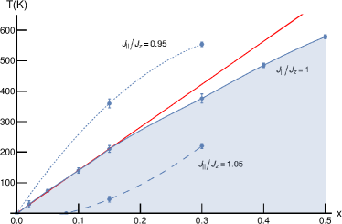
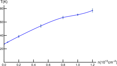
Figure 1: (left) Critical temperature for one-lattice ferromagnetism at half filling. The full blue line represents the isotropic case, which shows a linear behavior for small $x$, illustrated by the red line. The dashed and dotted lines are for two different cases of anisotropy, $J_{z}<J_{\parallel}$ and $J_{z}>J_{\parallel}$ , respectively. In these cases, the critical temperature is greatly affected, not only in terms of its value but also by becoming non linear. For $J_{z}<J_{\parallel}$ there is a critical concentration below which no ferromagnetic order exists. (right) Critical temperature for one-lattice ferromagnetism as a function of electron doping $n$. These results were obtained for $JS=0.4t$ and $x=0.1$. There is a steady increase of $T_{C}$ as the electronic density increases within the experimentally relevant regime.

III Adatoms in a single sublattice

III.1 Ferromagnetic critical Temperature

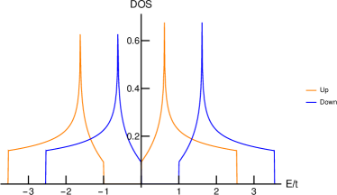
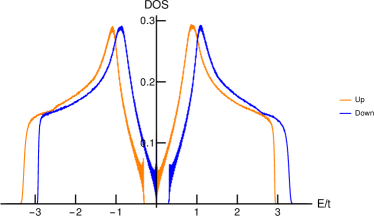
Figure 2: DOS at $T=0$ for two different concentrations of adatoms in a single sublattice: $x=0.5$ (left) and $x=0.15$ (right). For $x=0.5$, we obtain the expected result with gaps of value $JS$ for each spin projection. At lower adatom concentrations, the states become more uniformly distributed as the gaps decrease.

When placed on only one of the sublattices, the classical spins tend to align their orientations forming a ferromagnetic phase. In Fig. 1(left), the critical temperature is shown for a half-filled graphene lattice. In full, the isotropic case, $J_{\parallel}=J_{z}=J$, with $JS=t$ (Sengupta and Baskaran, 2008), shows a linear behavior for low impurity concentrations, with no signs of a critical concentration below which the ferromagnetic order is lost. This agrees with approximate results for a system of diluted spins interacting through a ferromagnetic, long ranged RKKY-like interaction (Szalowski et al., 2014). For $x<15\%$, the temperature dependence on $x$ is well described by the linear function $T_{C}\approx 1400x\,\text{(K)}$. The value of the coupling $JS$ obviously affects the critical temperature and is dependent on the impurity species used, with higher values resulting in higher $T_{C}$.

As already argued, we expect the real system not to be completely isotropic. We can easily change our model to encompass anisotropy, by distinguishing between the inplane and perpendicular directions: $J_{z}\neq J_{\parallel}$ (maintaining $J_{z}S=t$). We have found that even a small amount of anisotropy ($5\%$) substantially alters the $T_{C}$, as seen in Fig. 1(left). The dotted line refers to the anisotropic case with $J_{z}>J_{\parallel}$, where the critical temperature increases and becomes sub-linear. The case $J_{z}<J_{\parallel}$ (dashed line) the behavior seems to be superlinear. At low $x$, the suppression of $T_{C}$ is so strong that a critical concentration shows up. In this case, at $T=0$, the system undergoes a quantum phase transition as a function of $x$. In the very diluted limit at low enough temperatures, Kondo physics could eventually take over (Sengupta and Baskaran, 2008). This effect is not considered here.

The methodology followed here allows also to study the case of graphene away from half filling. In this situation, there should be more electrons available to couple different impurities. Based on this argument we can understand Fig. 1(right), where we show $T_{C}$ as a function of electron density, $n$, for a fixed concentration of magnetic adatoms $x=0.1$. The ferromagnetic phase becomes more stable as $n$ is increased. This holds even when the chemical potential is located inside the pseudogap that shows up in this phase, to be discussed below. Nevertheless, we expect the critical temperature to eventually reach a maximum value for some electronic density, decreasing towards zero after that. Our results show that this does not happen for electronic densities experimentally relevant.

The electronic density in graphene is easily changed by applying a bias gate voltage. Interestingly, the result of Fig. 1(right) provides proof of concept for a ferromagnetic transition tunable by electrical means: for a fixed temperature, tuning the electronic density through a gate voltage could induce ferromagnetic order on increasing voltage and paramagnetic behavior when the voltage is decreased.

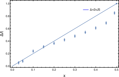
Figure 3: Spin resolved gap at $T=0$ for different one sublattice adatom concentrations. The line represents the value expected for a model where every site holds an adatom with smaller coupling.

III.2 Spectral properties

III.2.1 Single sublattice ferromagnetic phase

In the ferromagnetic phase the two electron-spin projections are not degenerate. When the impurities have a preferred direction, on average, one electron-spin projection will gain energy through interactions with the impurities, while the other will lose energy. At $T=0$, the system displays only a spin-resolved gap that decreases as $x$ is lowered, as shown in Fig. 2. Since there is never an overlap between the gaps in each spin projected DOS, the total DOS displays a pseudogap – a region of energies where a depletion of states is observed.

Let us consider the full single sublattice coverage, $x=0.5$. In this case the spin resolved gap is $JS$ and centered at $\pm JS/2$, depending on the spin projection. In fact, the system is now translational invariant and we can solve this case analytically in $k-$space (Daghofer et al., 2010). The energy bands are given by

$$E_{\text{$\mathbf{k}$},\uparrow} = \frac{1}{2}\left(-JS\pm\sqrt{J^{2}S^{2}+4|f_{\mathbf{k}}|^{2}}\right)$$ (13)

$$E_{\text{$\mathbf{k}$},\downarrow}=\frac{1}{2}\left(JS\pm\sqrt{J^{2}S^{2}+4|f_{\mathbf{k}}|^{2}}\right),$$ (14)

where $f_{\mathbf{k}}=\sum_{\bm{\delta}}\exp\left(i\mathbf{k}\cdot\bm{\delta}\right)$. We can use this to predict how the spin resolved gap decreases with impurity concentration. As we lower $x$, we can think that the effect of the coupling constant is diluted over every site of the sublattice, so that the system retains its translational symmetry. Now we can use the above equations with the modification $JS\rightarrow 2xJS$. In Fig. 3 we see that the results follow the predicted tendency, although the agreement is not complete. For high impurity concentrations the gap is lower than the predicted by this simple model. Both methods agree for concentrations below 20%.

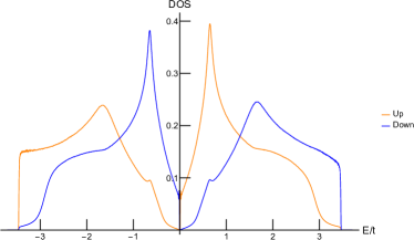
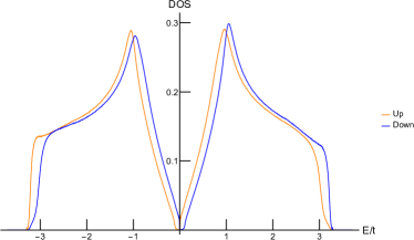
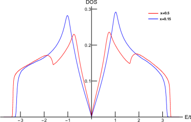
Figure 4: DOS at finite temperature, for different impurity concentrations on only one sublattice: (top) $T=0.72T_{C},\,x=0.5$; (mid) $T=0.82T_{C},\,x=0.15$. Temperature effects destroy the gaps in the spin projected DOS, creating Lifshitz tails. For high values of $x$ the spectrum for each spin is highly asymmetric.(bottom) DOS in the single sublattice paramagnetic regime for $x=0.5$ (red) and $x=0.15$ in (blue).

The finite temperature case is shown in Fig. 4, for $x=0.5$ (top) and $x=0.15$ (mid). We see that, for $0<T<T_{C}$, the gaps of each spin projection are no longer present, since Lifshitz tails effectively close the gaps. Both in this case and the $T=0$ case, there is always a region of energies where the electrons spin polarization is not balanced. This is particularly true around the zero energy, which means that any kind of electron doping will be polarized. In fact, since the states that form the Lifshitz tails are localized, we expect charge carriers to be 100% spin polarized in the pseudogap region. It is also worth mentioning the asymmetry observed for each spin projected DOS, especially evident at high concentrations. The main conclusion here is that, even though the spin resolved gaps vanish at finite temperature, there is still an imbalance between the two spin projections so that the pseudogap is still present. Ultimately, this feature is responsible for the energy gain in the ferromagnetic phase.

III.2.2 Single sublattice paramagnetism

In the paramagnetic regime, since the spins of the impurities are randomly oriented, there is no overall energy gain or loss for either electron-spin projection. Therefore, the system is now spin degenerate. In Fig. 4(bottom) we see that, similarly to the clean graphene case, the DOS vanishes linearly at $E=0$. In the clean limit, the DOS at low energies behaves as $\rho(E)=|E|/(hv)^{2}$, where $v$ is the Fermi velocity. An effective electron velocity $\tilde{v}$ may then be defined by linearly fitting the low energy numerical result in Fig. 4(bottom). We obtain, for $x=0.5$ a velocity of $\tilde{v}_{x=0.5}=0.66v$, and for $x=0.15$ the velocity $\tilde{v}_{x=0.15}=0.85v$. For $x=0.05$ we get a velocity $\tilde{v}_{x=0.05}=0.94v$, so we can actually infer a relation for the electronic velocity in this regime of low concentrations, $\tilde{v}_{x}\approx(1-x)v$. So, electrons around zero energy move slower when we include adatoms with their spins randomly orientated. We must keep in mind, however, that we are not taking into account the scattering of electrons in the adatoms (Irmer et al., 2018), which should further slow the movement of electrons on the lattice.

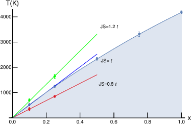
Figure 5: Critical temperatures for antiferromagnetism when both lattices are randomly occupied, on equal amount. The linear dependence for low $x$ is apparent.

IV Adatoms in both sublattices

IV.1 Critical Temperature

When magnetic adatoms are allowed to sit on both sublattices an antiferromagnetic regime is favored. In Fig. 5 we show the critical temperature below which an antiferromagnetic long range order starts to develop at mean field level, as a function of the impurity concentration $x$ for different values of coupling parameter $JS$. This case displays similar features to the single sublattice ferromagnetism, also predicting the absence of a critical concentration. The values of $T_{C}$, however, are one order of magnitude greater than the ferromagnetic critical temperature studied in Sec. III.1. For $JS=t$, the relation $T_{C}\approx 5000x\,\text{(K)}$ provides a good description of the linear behavior.

It is worth noting that Quantum Monte Carlo results for RKKY-like models lead to a much higher critical temperature for the antiferromagnetic case when the oscillatory component is not taken into account (Fabritius et al., 2010). So, MF seems to be a satisfactory approximation in this case. The colored lines in Fig. 5 show the $T_{C}$ follows the expected behavior with the change of the coupling constant $JS$: higher critical temperature for higher coupling, lower critical temperature for lower coupling. We have verified that $T_{C}$ has a quadratic dependence on $J$ (not shown), as found in Ref. (Rappoport et al., 2011).

IV.2 Spectral properties

As a general feature of antiferromagnetic order, we obtain that the two electron-spin projections are always degenerate. This can be understood as follows. Since impurities in different sublattices tend to align in opposite directions, electrons with one spin projection will gain energy in, say, sublattice A and lose energy in sublattice B. The same happens for the electrons with the other spin projection (with the roles of sublattices A and B interchanged). So, the two spin projections are equivalent, and thus we obtain a degenerate spin-resolved DOS. Throughout this section we consider $JS=t$.

IV.2.1 Full coverage antiferromagnetism

In order to gain insight into the obtained results, let us consider the fully covered, $x=1$ case. At $T=0$ we obtain a gap centered at zero energy, with value $2JS$, as shown in Fig. 6(left). Note that at $T=0$, when all thermal fluctuations are suppressed (i.e., at mean field level, all configurations of classical spins which deviate from perfect Néel order are inaccessible), we recover translational invariance due to the perfect long range antiferromagnetic order of the magnetic adatoms. In this limit we can solve the problem in $k$-space, as we did ferromagnetic ordering in Sec. III.2.1, in oder to obtain the spectrum and thus the DOS (Daghofer et al., 2010).

If we increase the temperature, but keep the full coverage $x=1$ case, we can isolate the effect of spin orientation disorder. The gap decreases significantly, with Lifshitz tails smoothing its edges, and the states get much more uniformly distributed along the whole energy spectrum, erasing the Van-Hove singularities. This effect is illustrated in Fig. 6(right). So, in contrast with the single sublattice ferromagnetic phase, the system opens an energy gap that survives at finite temperatures.

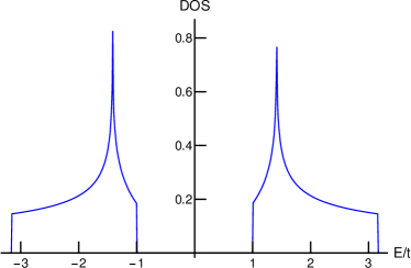
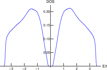
Figure 6: DOS for the full coverage antiferromagnetic phase at $T=0$ (left), when no thermal disorder exists, and $T=0.73T_{C}$ (right). Notice how singularities and band edges get smoothed out due to thermally induced disorder.

IV.2.2 Two-sublattices, partial coverage antiferromagnetism

Now we keep $T=0$, when perfect antiferromagnetic order is present, and study the effect of adatom position disorder by taking $x<1$. In Fig. 7(top) the DOS for $x=0.8$ and $x=0.1$ is shown. We see immediately that the energy gap decreases, although it is present at any concentration. For high impurity concentrations there are is a reconstruction of the DOS right next to the gap. The associated structures merge with the Van Hove singularities at $x\approx 0.5$. Increasing the temperature also destroys these features.

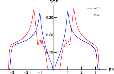
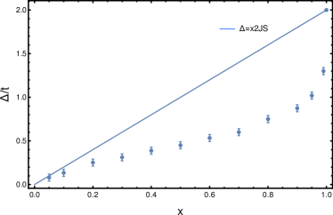
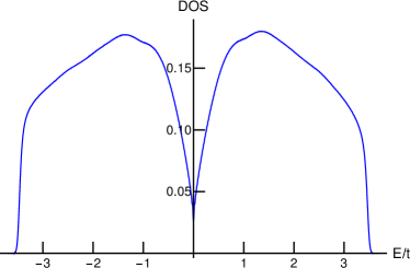
Figure 7: (top) DOS in the antiferromagnetic regime for $x=0.8$ (red) and $x=0.1$ (blue), at zero temperature. The energy gap decreases as we lower the value of $x$. At $x=0.8$ we can see the peak-like structures near the gap edges. (mid) Energy gap at $T=0$ for different concentrations. The line represents the value expected using a model where every site is occupied but with a weakened coupling. (bottom)DOS in the paramagnetic regime for $x=0.75$ with impurities on both sublattices. The DOS is finite at $E=0$

To understand the origin of these states let us go back to the full coverage case at $T=0$. There, the entire lattice is covered with impurities whose spins are oriented either up or down, depending on the sublattice they are located at. It is this full coverage that is responsible for the gap between $-JS$ and $JS$. If we remove a few impurities from the lattice, the gap should suffer only a slight perturbation. Additionally, these missing impurities create local states with midgap energies that start off as delta-like peaks in the DOS. Lowering the concentration broadens these sates and they eventually get included in the bands as the gap decreases. These impurity states are easily seen in the DOS, obtained with the recursion method, for example at $x\approx 0.99$ (not shown).

We can make an analysis similar to the that of Sec. III.2.1, spreading the effect of impurities over all sites, so that the obtained gap is given by $\Delta=x2JS$. In Fig. 7(mid) we can see how this model matches up with the results. As soon as we leave the full coverage case there is a steep decrease of gap relative to the $x2JS$ line. This is due to the states already mentioned that are created inside the gap, effectively reducing it. As the concentration decreases, the two approaches start to yield similar results. This is especially evident for concentrations under 10%. The energy gap present ensures the higher stability of the antiferromagnetic regime compared to the single sublattice ferromagnetic phase, surviving both adatom positioning and adatom-spin orientation disorders.

IV.2.3 Two-sublattices, paramagnetic phase

Above the critical temperature, the impurity spins are randomly oriented. The fact that now we have impurities on both sublattices, leads to a finite DOS at $E=0$, as shown in Fig. 7(bottom). This observation contrasts with the result obtained for the single sublattice case, shown in Fig. 4(bottom). As we lower $x$, the DOS in that point decreases. Below $x\approx 0.10$, we no longer have the required numerical resolution to conclude whether the DOS is still finite or not. The transition from finite DOS at $E=0$ in the paramagnetic phase to an energy gap in the antiferromagnetic one seems to be abrupt, since for a temperature $T=0.95T_{C}$ there is already a gap. So, most likely the gap is formed as soon as there is a preferred direction for the impurity spins, regardless of the value of the DOS at zero energy during the paramagnetic phase.

V Comparison with experiment

In this section we bring our model closer to experimental values to see if it can be used to understand some of the results obtained by Hwang et al. in their work concerning sulfur decorated graphene (Hwang et al., 2016). They report a sulfur (S) concentration of $x\approx 10\%$ and perform ARPES and magnetotransport measurements. Their main findings can be summarized as follows: temperature dependent depletion of states at the Fermi energy; magnetoresistance compatible with magnetic hysteresis.

We note that S atoms are not expected to be magnetic. However, in the case of Ref. (Hwang et al., 2016), there is a finite charge transfer from graphene to the S atoms that is measured experimentally and which, according to DFT calculations (Hwang et al., 2016), is responsible for the formation of a magnetic moment of $0.63\,\mu_{B}$ per S atom. Moreover, according to the same DFT calculations (Hwang et al., 2016), a possible position for the S atoms is to occur underneath graphene, between the top graphene layer and the buffer layer (a carbon layer with the same structure of graphene but without the $\pi$-bands due to strong hybridization with the SiC substrate). When the buffer layer and graphene are Bernal stacked, the two sublattices of the top graphene layer are no longer equivalent: one sublattice has buffer layer C atoms below, while the other sublattice occurs at the buffer layer hollow position where the S atoms sit (see Ref. (Hwang et al., 2016)).

Under the setup just presented, our model for one sublattice ferromagnetism may be seen as an adequate starting point. This model explains qualitatively the two main experimental observations of Ref. (Hwang et al., 2016). Regarding the magnetoresistance, and assuming that a ferromagnetic state develops as predicted by the present theory, the resistance should be maximized when the applied magnetic field reaches the value of the coercive field. In this situation the misalignment between the magnetization of different magnetic domains is maximum (so that the magnetization is zero), so electron scattering by impurity spins is also maximum. This explains the two peaks observed in the resistivity in Fig. 4D of Ref. (Hwang et al., 2016) at the two opposite values of the coercive field. This mechanism is particularly relevant in the pseudogap region (see Fig. 4), where it is expected that charge carriers at the Fermi level have a high degree of spin polarization in the direction of the local magnetization. As is shown below, the pseudogap is the relevant regime in the experiment of Ref. (Hwang et al., 2016).

We now turn to the depletion of states seen at the Fermi level in Ref. (Hwang et al., 2016). This result was interpreted as a signature of the opening of a gap at the Fermi level. This interpretation is hard to justify because of the lack of a nesting vector in the system, assuming the S atoms are randomly distributed, which is the relevant situation experimentally. In the present theory, the system does not open a true gap, but a pseudogap at the Dirac point, which could also explain the depletion of states near the Fermi level that is observed experimentally. In Fig. 8(left) we show the evolution of the pseudogap with the temperature. This pseudogap is a consequence of the impurities, which create a gap in the spectrum for each spin direction, one at positive energies and another at negative energies (as shown in Figs. 2 and 4), so there is a point where one of the spin resolved DOS is highly suppressed, creating this depletion of states relative to the clean graphene layer [shown as a dashed line in Fig. 8(left)]. The energy below which the depletion is most pronounced, signaled in Fig. 8(left) by the vertical dotted lines (roughly half the value of the pseudogap), becomes closer and closer to zero energy as we increase the temperature. This is the effect of disorder destroying the spin resolved gaps. On the other hand, on approaching the Dirac point, we see a region where the DOS is enhanced compared to the pristine case. In the latter case the DOS vanishes linearly whereas with impurities there is always a contribution from one of the spin projections.

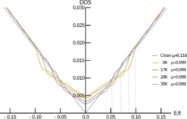
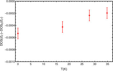
Figure 8: (left) Close up of the DOS around the pseudogap for several different temperatures in the case of single sublattice ferromagnetism for an impurity concentration $x=10\%$. The chemical potential was determined for each temperature in order to keep the electronic density fixed at $n=0.75\times 10^{13}\,\text{cm}^{-2}$(right) Difference between the DOS at the Fermi level for the sulfur doped graphene and the clean graphene at different temperatures. According to Ref. (Hwang et al., 2016), the charge carrier density in the clean case is $n=0.9\times 10^{13}\,\mbox{cm}^{-2}$, while in the sulfur decorated case it $n=0.75\times 10^{13}$cm^-2. We used these values to fix the Fermi energy in each case.

In order to make a closer comparison with the experimental results of Ref. (Hwang et al., 2016) regarding the depletion of states around the Fermi energy, we plot in Fig. 8 the difference between the DOS at the Fermi level for the S decorated case and the clean case. We determine the Fermi level by adjusting the charge carrier density to the reported values in Ref. (Hwang et al., 2016). For the clean graphene, they report $n=0.9\times 10^{13}\,\mbox{cm}^{-2}$, from which we get $\mu\simeq 0.116t$. Once the S impurities are added, Hwang et al. measure a change in the Fermi wave vector due to a charge transfer between S-atoms and the graphene system. Because of this charge transfer, the charge carrier density in graphene is lowered to $n=0.75\times 10^{13}\,\mbox{cm}^{-2}$. The obtained chemical potential is $\mu\simeq 0.099t$, with no significant change with temperature as indicated in Fig 8(left). The theory has a single adjustable parameter, the value of the coupling $JS$, which is fixed in order to reproduce the $T_{C}\sim 30\,\text{K}$ reported in Ref. (Hwang et al., 2016) at $x=10\%$ [a similar value has been used to produce Fig. 1(right)]. The negative values obtained for the DOS difference shown in Fig. 8 is indicative of a depletion of states with respect to the clean case, consequence of the shifting of the Fermi level towards lower energies. This observation agrees with the experimental finding. Moreover, we also see a temperature dependent depletion of states, where higher values of depletion occur as the temperature is lowered. This happens because the Fermi level is located at the edge of the pseudogap, whereas for higher temperatures it is already outside that region. This finding is again in agreement with the experimental result. In the present theory such depletion has no relation with a gap opening at the Fermi level.

VI Conclusions

We have studied the magnetic phase diagram of graphene decorated with magnetic adatoms located at the top position of the graphene lattice. Using a phenomenological $s$-$d$ model to couple the impurities with the underlying graphene electrons, and working with classical impurity-spins, we have treated the quantum degrees of freedom exactly and the classical variables at the mean-field level. This approach correctly takes into account effects of disorder on the electronic sector, due to both the random position of the impurities and the thermal fluctuation of the individual direction of the spins of the impurities. Moreover, the approach also takes into account the feedback of this disorder effects on the effective interaction between the impurity-spins.

Assuming that all the adatoms sit on a single graphene sublattice, a ferromagnetic phase has been found, with a critical temperature that depends linearly on the adatom concentration $x$, at low $x$. For an isotropic $s$-$d$ interaction, there is no sign of critical concentration $x_{c}$ below which ferromagnetism is lost. A critical $x_{c}$ shows up only when the coupling in the $xy$ plane is made stronger than the coupling in the $z$ direction. For a fixed $x$, we have determined the variation of the ferromagnetic critical temperature with charge carrier density, providing proof of concept for a ferromagnetic transition tunable by electrical means. Regarding the spectral properties of the electronic system, we have found that in the ferromagnetic phase, the spin polarization of the electrons is not balanced around zero energy. This is due to a pseudogap regime, where one polarization is strongly suppressed above zero energy, while the other is suppressed below. Since the suppressed component only contributes through Lifshitz tails, which are made of localized states, the spin polarization of charge carriers is expected to be close to 100% in the pseudogap region.

Allowing the adatoms to distribute randomly between the two sublattices, antiferromagnetism sets in, with the impurity spins ordering in opposite directions in the two sublattices. As in the ferromagnetic case, the low $x$ critical temperature also depends linearly on $x$. No critical $x_{c}$ is found below which the antiferromagnetic ordering is lost. Inside the antiferromagnetic phase, there is always a gap in the spectrum, despite adatom position and spin-orientation disorders. For adatom concentrations below $x\sim 10\%$, the gap depends linearly on $x$, but for higher values of $x$, strong deviation due to disorder are observed.

The results obtained here agree with several experimental observations where adatom decorated graphene has been shown to have a magnetic response (Xie et al., 2011; Garnica et al., 2013; Giesbers et al., 2013; Hwang et al., 2016; Tuček et al., 2017). Within the framework of the $s$-$d$ interaction, and taking into account the intrinsic disorder effects, the magnetic phases are found to be stable down to the lowest concentration of adatoms accessed here ($x\sim 1\%$). In particular, the present theory provides a qualitative understanding for the results of Ref. (Hwang et al., 2016), where a ferromagnetic phase has been found below $\sim 30\,\text{K}$ for graphene decorated with S-atoms.