Protostellar Outflows at the EarliesT Stages (POETS)

Centimeter continuum observations of protostellar jets have revealed the presence of knots of shocked gas where the flux density decreases with frequency. This spectrum is characteristic of nonthermal synchrotron radiation and implies the presence of both magnetic fields and relativistic electrons in protostellar jets. Here, we report on one of the few detections of nonthermal jet driven by a young massive star in the star-forming region G035.02$+$0.35. We made use of the NSF’s Karl G. Jansky Very Large Array (VLA) to observe this region at C, Ku, and K bands with the A- and B-array configurations, and obtained sensitive radio continuum maps down to a rms of 10 $\mu$Jy beam^-1. These observations allow for a detailed spectral index analysis of the radio continuum emission in the region, which we interpret as a protostellar jet with a number of knots aligned with extended 4.5 $\mu$m emission. Two knots clearly emit nonthermal radiation and are found at similar distances, of approximately 10,000 au, each side of the central young star, from which they expand at velocities of hundreds km s^-1. We estimate both the mechanical force and the magnetic field associated with the radio jet, and infer a lower limit of $0.4\times 10^{-4}$ M_⊙ yr^-1 km s^-1 and values in the range 0.7–1.3 mG, respectively.

1 Introduction

The centimeter continuum emission of ionized protostellar jets is a preferred tracer to image the outflow geometry, and, knowing the ionization fraction of local hydrogen gas, to quantify the mass-loss rate at scales from a few 10s to 1000s au of the central young star (e.g., Reynolds 1986; Tanaka et al. 2016). Radio jet properties have been recently reviewed by Anglada et al. (2018). The flux density ($S_{\nu}$) of radio jets typically increases with frequency ($\nu$) within a few 1000s au of the central star ($S_{\nu}\propto\nu^{\alpha}$), showing a partially opaque spectral index ($0<\alpha<2$). These spectra are interpreted as thermal free-free emission from ionized particles accelerated within their own electric field. Notably, along the axis of a few radio jets, the spectrum is occasionally inverted at the loci of bright knots of ionized gas (e.g., Rodríguez et al. 2005; Carrasco-González et al. 2010; Moscadelli et al. 2013; Rodríguez-Kamenetzky et al. 2016; Osorio et al. 2017), showing spectral index values much less than the optically thin limit ($-0.1$). These spectra are interpreted as evidence for (nonthermal) synchrotron emission from strong jet shocks against the ambient medium, where ionized particles would be sped up to relativistic velocities via diffusive shock acceleration (e.g., Padovani et al. 2015, 2016).

For the prototypical synchrotron jet HH 80–81, Carrasco-González et al. (2010) detected linear polarization of the centimeter continuum emission for the first time, proving that the negative slope of the radio spectrum is due to synchrotron radiation. Polarized maser emission associated with protostellar outflows provides further evidence for the presence of magnetic fields, and observations of maser cloudlets at milli-arcsecond resolution show a strong correlation between the local orientation of proper motion and magnetic field vectors (e.g., Surcis et al. 2013; Sanna et al. 2015; Goddi et al. 2017; Hunter et al. 2018). In this Letter, we report on one of the very few detections of a nonthermal jet emitted by a young massive star, discovered in the star-forming region G035.02$+$0.35 as part of the Protostellar Outflow at the EarliesT Stage (POETS) survey (Moscadelli et al. 2016; Sanna et al. 2018, hereafter Paper I).

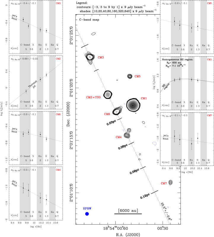
Figure 1: Extended radio jet emission driven by source CM2 in G035.02$+$0.35. Middle Panel: continuum map obtained with the A-configuration of the VLA at C-band (without constraints on uv-coverage). Contour levels, at multiple of the 1 $\sigma$ rms, are indicated on top; levels higher than 10 $\sigma$ are drawn in grey shades. The beam size is shown in the bottom left corner. A scale bar in units of au is drawn near the bottom axis. The field-of-view covers the radio continuum sources detected within 0.1 pc from CM2 (CM8 in Fig.3), whose centimeter spectral index ($\alpha$) traces radio thermal jet emission (from Paper I). Labels are indicated in red near each source. Components CM3, CM4, and CM6 are aligned along a position angle of 25.5$\degr$ $\pm$ 0.6$\degr$ with respect to CM2 (dotted line), tracing the location of four jet’s knots. Ticks are marked along the jet direction at steps of 6000 au from CM2. Side Panels: centimeter spectral energy distribution of radio components surrounding CM2. Each plot shows the logarithm of the integrated flux (in mJy) as a function of the logarithm of the observed frequency (in Hz) for four data points. Details for CM2 were presented in Paper I. Different frequency bands are labeled near the bottom axis together with the reference wavelength; grey shades mark the boundary of each band. The spectral index values ($\alpha$) and their uncertainties, derived from a linear fit of the four data points, are specified in the upper left corner of each panel. Assuming an electron temperature of 10⁴ K, the spectral energy distribution of source CM1 is well reproduced by a model of homogeneous H ii region with: Strömgren radius (R_S) of 630 au, number of Lyman photons (N_Ly) of 10^45.85 s^-1, electron density (n_e) of 8.8 $\times$ 10⁴ cm^-3, and emission measure (EM) of 4.8 $\times$ 10⁷ pc cm^-6.

The star-forming region G035.02$+$0.35 hosts diverse stages of stellar evolution, including a hot molecular core (HMC) near to a hyper compact (HC) H ii region (e.g., Brogan et al. 2011; Beltrán et al. 2014). At a parallax distance of 2.33 kpc from the Sun (Wu et al. 2014), the entire region emits a bolometric luminosity of 1–3 $\times$ 10⁴ L_⊙ (Beltrán et al. 2014; Towner et al. 2018, in prep.). G035.02$+$0.35 was surveyed with the IRAC instrument onboard of Spitzer and classified as an extended green object (EGO) associated with bright 4.5 $\mu$m emission, which is a tracer of ambient gas shocked by early outflow activity (Cyganowski et al. 2008, 2009; Lee et al. 2013). Cyganowski et al. (2011) made a census of the 8 GHz continuum sources at the center of the IR nebula with the B-configuration of the Very Large Array (VLA). They identified 5 compact radio sources above a threshold of 100 $\mu$Jy beam^-1. Here, we make use of the longest VLA baselines at 6, 15, and 22 GHz (C, Ku, and K bands, respectively) to image the continuum emission at a sensitivity of 10 $\mu$Jy beam^-1. Observation information was presented in Paper I and is summarized in Table 1. We have performed a detailed spectral index analysis for each radio continuum component and we have identified an extended radio jet with nonthermal knots. This radio jet is driven by the HMC source at the base of the IR nebula.

Table 1: Summary of VLA observations towards G035.02$+$0.35 (code 14A-133).

Band	$\nu_{\rm center}$	BW	Array	HPBW	RMS noise
	(GHz)	(GHz)		(′′)	($\mu$Jy beam-1)
C	6.0	4.0	A	0.338	9.0
Ku	15.0	6.0	A	0.138	9.0
K	22.2	8.0	B	0.308	9.0

Table 2: Continumm fluxes of centimeter sources in G035.02$+$0.35.

Component	Band	R.A. (J2000)	Dec. (J2000)	S${}^{uv}_{int}$
		(h m s)	(∘ ′ ′′)	(mJy)
CM1	C	18:54:00.492	02:01:18.34	12.092 / 12.747
	Ku	18:54:00.492	02:01:18.34	12.432
	K	18:54:00.492	02:01:18.34	11.837
CM2	C	18:54:00.648	02:01:19.36	0.825
	Ku	18:54:00.649	02:01:19.42	1.584
	K	18:54:00.648	02:01:19.42	2.036
CM3	C	18:54:00.764	02:01:22.96	0.474 / 0.337
	Ku	18:54:00.764	02:01:22.90	0.276
	K	18:54:00.764	02:01:22.96	0.264
CM4	C	18:54:00.528	02:01:15.46	0.061 / 0.054
	Ku	18:54:00.532	02:01:15.52	0.035
	K	18:54:00.536	02:01:15.40	0.032
CM5	C	18:54:00.508	02:01:21.10	0.061 / 0.049
	Ku	18:54:00.508	02:01:21.10	0.042
	K	18:54:00.508	02:01:21.04	0.046
CM6	C	18:54:00.592	02:01:17.74	0.262 / 0.290
	Ku	18:54:00.592	02:01:17.74	0.257
	K	18:54:00.596	02:01:17.68	0.199
CM7	C	18:54:00.252	02:01:10.96	0.031 / 0.024
	Ku	18:54:00.252	02:01:10.90	0.017
	K	18:54:00.252	02:01:10.90	0.026
CM8	C	18:54:01.657	02:01:54.04	0.055 / 0.068
	Ku	18:54:01.657	02:01:53.98	0.049
	K	…	…	$<0.045$

2 Results

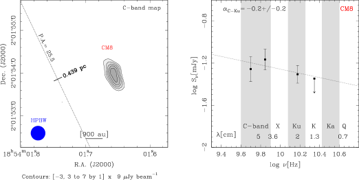
Figure 3: Radio continuum map (left) and spectral index analysis (right) of component CM8, which is located to the NE of CM2, at a projected distance of $38\aas@@fstack{\prime\prime}86$. Same symbols and labels as in Fig. 1. The spectral index of CM8 was computed with a linear regression fit between the C and Ku bands only; at K band we provide an upper limit of 5 $\sigma$.

In Fig. 1, we present a radio continuum map at C band of G035.02$+$0.35, obtained at a resolution of $0\aas@@fstack{\prime\prime}34$. For a direct comparison with previous observations, we adopt the same labeling of radio continuum components introduced by Cyganowski et al. (2011, from CM1 to CM5), and extend the source numbering to the new radio components detected in this paper (CM6, CM7, and CM8). We detect eight, distinct, radio continuum sources at multiple frequencies above a threshold of 27 $\mu$Jy beam^-1 (3 $\sigma$); six of them are distributed within a radius of 0.1 pc from CM2. CM2 coincides in position with the brightest millimeter peak in the region, and the richest site of molecular line emission, named core A in Beltrán et al. (2014, their Figs. 2 and 4). The spectral energy distribution of CM2 has a constant spectral index of 0.69 between 1 and 7 cm, which is consistent with thermal jet emission from a young star. Its radio luminosity, of approximately 5 mJy kpc² at 8 GHz, is indicative of an early B-type young star, according to the correlation between radio jet and bolometric luminosities (e.g., Fig. 6 of Paper I). The radio continuum emission from CM2 was previously presented in Paper I (see also Fig. 3 of Cyganowski et al. 2011). In the following, we comment on the radio continuum components detected near to CM2.

In Table 2, we list the integrated fluxes at C, Ku, and K bands for each radio continuum component. These fluxes were computed within a common uv-distance range of 40–800 k$\lambda$, as described in Paper I, and the C-band data were split in two sub-bands of 2 GHz each. In the side panels of Fig. 1, we analyze the spectral energy distribution of each radio component.

CM1 is the brightest radio continuum source in the region, and it is located to the west-southwest of CM2, at a projected distance of $2\aas@@fstack{\prime\prime}55$ (or 5944 au). Its spectral energy distribution is characteristic of a photoionized H ii region which is hyper compact, with an angular size (best fit) of $0\aas@@fstack{\prime\prime}54$ corresponding to a Strömgren radius (R_S) of 630 au. This size is consistent with the (deconvolved) size obtained directly by fitting the observed image. The four data points are consistent with a homogeneous H ii region model with constant electron density and temperature, fixed to $10^{4}$ K (see Fig. 1). This model implies a number of Lyman photons (N_Ly) of 10^45.85 s^-1, and an electron density (n_e) and emission measure (EM) of 8.8 $\times$ 10⁴ cm^-3 and 4.8 $\times$ 10⁷ pc cm^-6, respectively. The number of Lyman photons corresponds to that emitted by a ZAMS star of spectral type between B1–B0.5 and bolometric luminosity of 8–9 $\times$ 10³ L_⊙ (e.g., Thompson 1984). These values are consistent with those reported by Cyganowski et al. (2011) after scaling their distance (3.43 kpc) to the current value (2.33 kpc).

The spectral index of components CM3 to CM7 was computed with the linear regression fit drawn in each panel of Fig. 1, where we also report the spectral index values with 1 $\sigma$ uncertainty. Notably, CM3 and CM4 have negative spectral slopes steeper than the optically thin limit. Their spectra are consistent with nonthermal radiation within a confidence level of 3 $\sigma$. Instead, the spectral index of CM5, CM6, and CM7 is consistent with optically thin free-free radiation within 1 $\sigma$.

In particular, the peak positions of radio components CM2, CM3, CM4, and CM6 are well-aligned on the plane of the sky. The four points fit a straight line which is oriented at a position angle of 25.5$\degr$ with a small uncertainty of 0.6$\degr$ (dotted line in Fig. 1). CM3 and CM4 are located each side of CM2 at a similar distance of $4\aas@@fstack{\prime\prime}00$ (9320 au) and $4\aas@@fstack{\prime\prime}29$ (9996 au), respectively; CM6 is located closer to CM2 at a distance of $1\aas@@fstack{\prime\prime}83$ (4252 au). Unlike CM2, the radio continuum emission from CM3, CM4, and CM6 does not coincide with compact dust emission (e.g., Fig. 2 of Beltrán et al. 2014). The linear distribution and the spectral index analysis support the following interpretation: CM2, CM3, CM4, and CM6 trace the same ionized jet, with CM2 pinpointing the origin where the central powering source is surrounded by partially opaque plasma, while CM3 and CM4 arise from two shocks emitting synchrotron radiation located symmetrically with respect to CM2, and CM6 marks a shock emitting optically thin free-free radiation located closer to CM2.

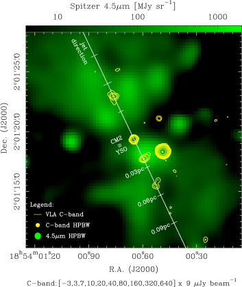
Figure 2: Comparison between the radio jet emission driven by source CM2 (yellow contours) and the 4.5 $\mu$m nebula imaged by Spitzer in the region (green scale). The radio continuum map is the same drawn in Fig. 1, together with the jet direction and ticks (dotted white line). Contour levels are indicated to the bottom. The logarithmic (green) scale of the 4.5 $\mu$m emission is drawn in the top wedge. The enhanced resolution (HPBW) of the Spitzer map is shown in the bottom left corner (Sect. 2 for details).

Table 3: Properties of the thermal radio jet at the position of CM2.

Assumed parameters

Radio observables

Jet energetics

$\epsilon$

qT

qx

$F(\alpha)$

x0

$T$

$\nu_{m}$

$\nu$

$S_{8GHz}$ $\times$ $d^{2}$

$\alpha$

$\psi$

$i$

$V_{\rm jet}$

$\dot{M}_{\rm jet}$

$\dot{p}_{\rm jet}$

(K)

(GHz)

(GHz)

(mJy $\times$ kpc2)

($\degr$)

($\degr$)

(km s-1)

(M⊙ yr-1)

(M⊙ yr-1 km s-1)

1

0

0

1.33

1

104

¿26

8.0

1.01 $\times$ 2.332

0.6

6

60–90

200

0.2$\cdot$10-6

0.4$\cdot$10-4

0.1

600

0.5$\cdot$10-5

3.2$\cdot$10-3

In Fig. 2, we provide further evidence supporting the interpretation of a single radio jet, by comparing the spatial distribution of the radio continuum emission with the morphology of the 4.5 $\mu$m emission (another typical outflow tracer). The 4.5 $\mu$m map has been previously presented in Beltrán et al. (2014, their Fig. 2), who processed the Spitzer/IRAC data making use of the high resolution deconvolution algorithm by Velusamy et al. (2008). The EGO has a bipolar structure centered on CM2 and oriented in the direction of the radio continuum sources CM3, CM4, and CM6, which, in turn, appear to bisect the EGO. Additional arguments in favor of the jet interpretation are discussed in Appendix A, based on the proper motions of CM3 and CM4 with respect to CM2, and the elongated morphology of the continuum emission. In the following, we refer to the position angle of 25.5$\degr$ as the jet axis.

We also detect two additional radio continuum sources farther from CM2 (in projection) along the axis of the jet, CM7 (Fig. 1) and CM8 (Fig. 3). CM7 is $10\aas@@fstack{\prime\prime}29$ (0.116 pc) away from CM2 and only slightly offset at a position angle of 35$\degr$. CM8 is $38\aas@@fstack{\prime\prime}86$ (0.439 pc) away from CM2 to the northeast and elongated in the direction of the jet axis. They could mark farther knots of (optically thin) ionized gas caused by the jet passage.

The position of CM5, well away from the jet axis, argues that it traces a separate object. Its radio continuum flux, which is approximately constant between 1 and 7 cm, is consistent with a small, optically thin, H ii region (R_S $\lesssim$ 100 au). The ionized flux can be reproduced with a number of Lyman photons of about 10^43.45 s^-1 (e.g., Eq. 1 of Cyganowski et al. 2011), coming from a young star with a spectral type later than B2.5 and a bolometric luminosity of approximately 1 $\times$ 10³ L_⊙.

3 Discussion

In the following, we quantify the mass loss ($\dot{\rm M}_{\rm jet}$) and momentum ($\dot{\rm p}_{\rm jet}$) rates of the radio jet, as well as estimate the magnetic field strength (B_min) at the position of the synchrotron knots.

First, we apply Eq. (1) of Sanna et al. (2016) to estimate the mass ejected per unit time at the position of CM2, as a function of the flux density ($S_{\rm\nu}$), frequency ($\nu$), and spectral index of the continuum emission ($\alpha$), the turn-over frequency of the radio jet spectrum ($\nu_{\rm m}$), the semi-opening angle of the radio jet ($\psi$), its inclination with respect to the line of sight ($i$), and the expanding velocity of the ionized gas ($V_{\rm jet}$). We assume that the radio jet can be approximated by a conical flow, where gas is isothermal at a constant temperature of 10⁴ K, and it is uniformly and fully ionized (x₀ $=$ 1). In Table 3, we list the values used in the calculation.

Values of spectral index and integrated flux density for CM2 at 8.0 GHz are obtained from Table 3 of Paper I. The spectral index is approximated to 0.6 within the uncertainty of its measurement, and it is consistent with the assumption of conical flow (e.g., Eq. 5 of Anglada et al. 2018). A lower limit to the turn-over frequency is set by the higher frequency of the K-band observations (26 GHz), although the mass loss rate does not depend on the turn-over frequency for $\alpha\,=0.6$. We have estimated the jet opening angle ($2\times\psi$) drawing the tangents to the 3 $\sigma$ contours of CM3 from the peak position of CM2. These tangents are approximately symmetric with respect to the jet axis and define an aperture of 12$\degr$. The extended bipolar geometries of the radio continuum emission and IR nebula suggest that the jet axis is nearly perpendicular to the line of sight, although a direct measurement is not available. We assume an inclination ($i$) in the range 60$\degr$–90$\degr$ which changes the mass loss rate by less than a few percent. We further consider a lower limit to the jet velocity of 200 km s^-1, based on the proper motion analysis in Appendix A which provides an estimate of the shock velocities.

These values imply a jet mechanical force ($\dot{\rm p}_{\rm jet}$) at its origin of $0.4\times 10^{-4}$ M_⊙ yr^-1 km s^-1. However, in the calculation we have followed a conservative approach, assuming that the jet is hundred percent ionized; this assumption implies a lower limit of the mass loss (and momentum) rate which is inversely proportional to the ionization fraction. On the contrary, previous statistically studies of radio jets assumed a low ionization fraction in the range 10–20% (e.g., Purser et al. 2016; Anglada et al. 2018), which is supported by NIR observations (e.g., Fedriani et al. 2018). Moreover, in the case of a massive young star undergoing an accretion burst (S255 NIRS3), Cesaroni et al. (2018) showed that the radio thermal jet emission is produced by a low ionization degree ($\sim$ 10%). For this reason, in Table 3 we also estimate the radio jet properties assuming that its gas is mostly neutral, and it is moving at high velocities of 600 km s^-1. Rodríguez-Kamenetzky et al. (2016) showed that jet velocities of the order of 500–600 km s^-1 might be needed to efficiently promote particles acceleration (and synchrotron emission) in the shocks against the ambient medium. Under this conditions, we estimate an upper limit to the jet mechanical force of $3.2\times 10^{-3}$ M_⊙ yr^-1 km s^-1. This value is consistent with the relationship between mechanical force and radio luminosity of jets reported in Fig. 9 of Anglada et al. (2018), where a low ionization fraction was assumed.

Second, we estimate the minimum-energy magnetic field strength, B_min, which minimizes together the kinetic energy of the relativistic particles and the energy stored in the magnetic field. For a direct comparison of B_min in another radio synchrotron jet, we follow the same calculations of Carrasco-González et al. (2010). We make use of the classical minimum-energy formula, valid in Gaussian CGS units: B_min $=$ $[4.5c_{12}(1+k)\rm L_{R}]^{2/7}(R^{3}\phi)^{-2/7}$, where $L_{R}$ is the synchrotron luminosity measured in a spherical source of radius R. The filling factor, $\phi$, accounts for a smaller region of synchrotron radiation with respect to the source size. The two coefficients, $c_{12}$ and $k$, depend on the integrated radio spectrum and on the energy ratio among relativistic particles in the region, respectively (e.g., Govoni & Feretti 2004; Beck & Krause 2005).

In Table 4, we list the values used to calculate B_min. We estimate the magnetic field strength for sources CM3 and CM4 separately, and obtain values of 1.3 mG and 0.7 mG, respectively. On the one hand, these values are a factor 6–3 times higher than the magnetic field strength (0.2 mG) estimated by Carrasco-González et al. (2010) in the radio jet HH 80–81. These differences might be consistent with the uncertainty of the prior assumptions, such as $\phi$ and $k$. On the other hand, since the synchrotron knots in HH 80–81 are located 10 times further away from their exciting protostar than CM3 and CM4 are from CM2, the magnetic field strength might reasonably be lower for that case (e.g., Seifried et al. 2012). Interestingly, in the synchrotron component of the jet driven by NGC6334I–MM1B, OH maser emission provides an independent Zeeman measurement of the magnetic field strength locally (0.5–3.7 mG), which is consistent with the values estimated above (Brogan et al. 2016, 2018; Hunter et al. 2018). We further note that the 6.7 GHz CH₃OH masers detected at the position of CM2 show linearly polarized emission, and this emission supports a magnetic field orientation aligned with the direction of the jet axis (Surcis et al. 2015, their Fig. 5).

Although more data are required to fully confirm the proposed interpretation in terms of a single jet with synchrotron knots, overall these findings suggest that G035.02$+$0.35 can provide a preferred laboratory for studying the role of magnetic fields in the acceleration and collimation of protostellar jets (e.g., Kölligan & Kuiper 2018).

Table 4: Minimum-energy magnetic field strength in the radio jet.

	$c_{12}$	$k$	LR	$R$	$\phi$	$B_{\rm min}$
	($10^{7}$)		($10^{27}$ erg s-1)	($10^{15}$ cm)		(mG)
CM3	1.395	40	13.6	6.2	0.5	1.3
CM4	1.398	40	1.2	5.4	0.5	0.7

Appendix A Proper motions and elongation of the radio jet

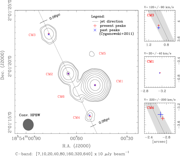
Figure 4: Proper motion analysis of the radio continuum sources in G035.02$+$0.35. Left Panel: 2014 C-band map (contours) processed under similar conditions of uv-coverage and restoring beam size as the 2009 X-band map of Cyganowski et al. (2011), for comparison. Contour levels are indicated to the bottom at multiples of the 1 $\sigma$ rms; the beam size is shown in the bottom left corner. Radio continuum labels, jet axis, and ticks are the same as in the Fig. 1. Red and blue crosses mark the centroid positions of CM1, CM2, CM3, and CM4 in May 2014 and 2009, respectively, as obtained from a two-dimensional Gaussian fit of the C- and X-band maps (X-band positions from Table 2 of Cyganowski et al. 2011). Individual centroids have been registered by aligning the positions of CM2 in 2014 and 2009. Right Panels: zoom-in near to the centroids of CM3 (top), CM1(middle), and CM4 (bottom). The extent of each map is the same; angular offsets (in arcsec) are referred to the phase center. The size of each cross quantifies the uncertainty in the centroid position (see Sect. A). For CM1, CM3, and CM4, we indicate the magnitude of the proper motions (and uncertainty) inferred from the displacement of their centroids between the two epochs. The dotted line and the gray shadow mark the jet axis and its 3 $\sigma$ uncertainty ($\pm 1.8\degr$), respectively.

In this section, we compare our C-band observations with the X-band observations reported by Cyganowski et al. (2011), with the aim to reveal the proper motion of the radio jet and provide further proof that CM2, CM3, CM4, and CM6 belong to the same radio jet.

Cyganowski et al. (2011) observed G035.02$+$0.35 with the B configuration of the VLA at X-band (3.6 cm) on 2009 May 7–14, five years before our C-band observations. In their Table 2, they reported the centroid positions of CM1, CM2, CM3, and CM4 at that epoch, obtained from a two-dimensional Gaussian fit (CM5 was not fitted because only marginally detected). The X-band map had a beam size of $1\aas@@fstack{\prime\prime}05\times 0\aas@@fstack{\prime\prime}96$, oriented at position angle of $8.9\degr$, and a rms of 0.03 mJy beam^-1.

To compare the C- and X-band observations directly, we have used the task clean of CASA and imaged the C-band dataset excluding uv-distances greater than 300 k$\lambda$, to approximate the uv-coverage of the X-band dataset. We have also applied a natural weighting and set a restoring beam size equal to that of the X-band map. The resulting C-band map (Fig. 4) well resembles that at X-band presented in Fig. 1 of Cyganowski et al. (2011), where the continuum component CM6 is blended with CM1 and CM2. Notably, with respect to Fig. 1, the continuum emission in Fig. 4 shows a higher degree of elongation in the direction of the jet axis, meaning that we have retrieved extended jet emission resolved out with the longest baselines (i.e., greater uv-distances). In particular, the deconvolved (Gaussian) size of sources CM2 ($\lesssim 0\aas@@fstack{\prime\prime}5\times 0\aas@@fstack{\prime\prime}2$ at a position angle of $17\degr\pm 10\degr$) and CM3 ($\lesssim 0\aas@@fstack{\prime\prime}6\times 0\aas@@fstack{\prime\prime}1$ at a position angle of $21\degr\pm 5\degr$) proves a strong elongation of the radio continuum emission (a factor $\geq 2.5$) and that this elongation is consistent with the estimated direction of the jet, within the uncertainties.

In Fig. 4, we compare the position of the continuum sources on May 2014 (red crosses) and May 2009 (blue crosses). Similar to Cyganowski et al. (2011), we have fitted sources CM1, CM2, CM3, and CM4 with a two-dimensional Gaussian distribution in order to determine their centroid positions (Table 5). We have then compared the relative position of these centroids between the two epochs by aligning the positions of CM2, which corresponds to the origin of the radio jet.

In the right panels of Fig. 4, we enlarge the regions around CM1, CM3, and CM4 for a detailed analysis of the centroid positions. The size of the red and blue crosses quantifies the positional uncertainty of the Gaussian fits; this uncertainty is calculated from the following formula: $(FWHM/2)\times(\sigma/I)$, where $I$ and $\sigma$ are the peak intensity and the rms noise, respectively (e.g., Reid et al. 1988). The FWHM is conservatively taken equal to the common beam size of the C- and X-band maps. These plots show that CM3 and CM4 are moving away from the position of CM2 and are consistent with the jet axis (dotted line) within a confidence level of about 2 $\sigma$. The gray shadow marks the 3 $\sigma$ uncertainty of the jet axis. This result gains more strength when compared to the position of CM1, which has not changed in time significantly, and further supports the intepretation that CM3 and CM4 belong to the same radio jet which originates at the position of CM2.

In the right panels of Fig. 4, we also report the magnitude of the proper motions for CM1, CM3 and CM4 with respect to CM2, estimated from the displacement of their centroids (column 9 of Table 5). For CM3, we calculate a velocity of 120 km s^-1 with an uncertainty of 90 km s^-1. For CM4, we calculate a velocity of 220 km s^-1 with an uncertainty of 200 km s^-1. These values are consistent with the proper motions of nonthermal knots measured in other sources (e.g., Rodríguez-Kamenetzky et al. 2016), providing an estimate of the shock velocities and a lower limit on the underlying jet velocity.

Table 5: Proper motion study of CM1, CM3, and CM4 with respect to CM2.

Component	Epoch	R.A. (J2000)	$\Delta$x	Dec. (J2000)	$\Delta$y	Vx	Vy	$\rm|V|$	P.A.
		(h m s)	(′′)	(∘ ′ ′′)	(′′)	(mas yr-1)	(mas yr-1)	(km s-1)	(∘)
CM1	May 2009	18:54:00.49098	0.001	02.01:18.292	0.001	…	…	…	…
	May 2014	18:54:00.48936	0.001	02.01:18.332	0.001	–2 $\pm$ 2	1 $\pm$ 2	20 $\pm$ 40	$-63^{+41}_{-18}$
CM2	May 2009	18:54:00.6498	0.010	02.01:19.32	0.010	…	…	…	…
	May 2014	18:54:00.6489	0.006	02.01:19.354	0.006	0	0	0	…
CM3	May 2009	18:54:00.766	0.030	02.01:22.82	0.030	…	…	…	…
	May 2014	18:54:00.765	0.010	02.01:22.91	0.010	–1 $\pm$ 6	11 $\pm$ 6	120 $\pm$ 90	$-5^{+29}_{-27}$
CM4	May 2009	18:54:00.523	0.060	02.01:15.60	0.060	…	…	…	…
	May 2014	18:54:00.519	0.020	02.01:15.55	0.020	–10 $\pm$ 12	–17 $\pm$ 12	220 $\pm$ 200	$210^{+25}_{-43}$