Small-scale chemical abundance analysis in a blue compact dwarf galaxy SBS 1415+437

Abstract

We use integral field spectroscopic (IFS) observations from Gemini Multi-Object Spectrograph-North (GMOS-N) to analyse the ionised gas in the principal star-forming region in the blue compact dwarf galaxy SBS 1415+437. The IFS data enable us to map the weak auroral line [O iii] $\lambda$4363 at a spatial scale of $\sim$6.5 pc across a region of $\sim$143 $\times$ 143 pc². This in turn allows us to use the robust direct T_e-method to map the ionic and elemental abundances of nitrogen (N) along with the alpha-elements, oxygen (O), neon (Ne), sulphur (S) and argon (Ar). We utilise these abundances to map the relative abundances of N, Ne, S and Ar with respect to O. We segment this predominantly photoionised region of study into elliptical annuli on the basis of the H$\alpha$ flux distribution to study the variation of chemical abundances and their ratios, and find no significant chemical variation. We also perform chemical abundance analysis on the integrated spectra of the region under study and elliptical annuli within it. We find that the inferred abundances are in agreement with the median of the abundances obtained from the chemical abundance maps of the principal star-forming region and the mapped values within annuli.The finding has important implications for direct comparison with high-redshift observations, where spatial resolution is not available, and for a consistent approach to track chemical evolution across cosmic time.

1 Introduction

Our understanding of the chemical evolution of the Universe relies on our knowledge of the origin and distribution of elements in the nearby and distant Universe. The study of abundance of oxygen (O) and its distribution is important because it is the third most abundant element in the Universe after hydrogen and helium, and hence acts as a good proxy to the total metal-content of a star-forming system. The abundances of other elements and their relative abundance with respect to oxygen tell us about the nucleosynthetic origin of these elements. For example, $\alpha$-elements such as neon (Ne), sulphur (S) and argon (Ar) are thought to be produced in massive stars along with oxygen (see e.g. Woosley & Weaver, 1995), while nitrogen (N) is thought to form in massive, as well as intermediate mass stars, though there have been many debates on its origin (see e.g. Kumari et al., 2018, and references therein). Various observational studies have explored the distribution of these elements in stars and gas within star-forming and quiescent systems (see e.g. Vílchez & Iglesias-Páramo, 1998; Henry & Worthey, 1999; López-Sánchez et al., 2007; García-Benito et al., 2010; Monreal-Ibero et al., 2011; Lind et al., 2011; Berg et al., 2013; López-Hernández et al., 2013; Berg et al., 2015). These studies show that the distribution of chemical abundances may vary over both small sub-galactic scales or large galactic scales within galaxies (see e.g. Henry & Worthey, 1999; Kewley et al., 2010; Pilkington et al., 2012; James et al., 2015). The abundance pattern tells us about various constituents of chemical evolutionary models such as star-formation history, chemical enrichment, merger events, gas dynamics and stellar-populations.

Table 1: General Properties of SBS 1415+437

Parameter	SBS 1415+437
Morphological Type	BCD
R.A. (J2000.0)	14h17m01.4s
DEC (J2000.0)	+43d30m05s
Redshift (z)a	$\sim$0.00203
Distance (Mpc)b	13.6
Helio. Radial Velocity(km s-1)a	609 $\pm$ 2
E(B-V)c	0.0077 $\pm$ 0.0003
Mstellar (107 M⊙)d	17 $\pm$ 3
Mmolecular (107 M⊙)d	7.6 $\pm$ 2.3
M${}_{\rm{H\textsc{i}}}$ (107 M⊙)d	6.8 $\pm$ 0.7
a Taken from NED
b Aloisi et al. (2005)
c Foreground galactic extinction (Schlafly & Finkbeiner, 2011)
d Lelli et al. (2014)

Table 2: GMOS-N IFU observing log for SBS 1415+437

Grating	Central wavelength (Å)	Wavelength Range (Å)	Exposure Time (s)	Average Airmass	Standard Star
B600+_G5307	4700	3250 – 6118	2$\times$1850	1.098, 1.092	Wolf1346
R600+_G5304	6900	5443 – 8361	2$\times$1800	1.161, 1.121	Wolf1346

Studies of large and small-scale chemical variation have been revolutionised with the advent of integral field spectroscopy (IFS) which allows us to derive spatially-resolved spectroscopic properties of the star-forming systems (Pérez-Montero et al., 2011; Sánchez et al., 2012; Westmoquette et al., 2013; Kehrig et al., 2013; Ho et al., 2015; Belfiore et al., 2017). For example the spectrum of a star-forming galaxy, or an H ii region, contains a plethora of emission lines. IFS enables us to map emission lines across the star-forming galaxy, or region within a galaxy, depending on the field-of-view (FOV) of instruments, and therefore map the physical properties encoded in those emission lines. This simultaneous observation in wavelength and space is key to an efficient study of the distribution of chemical abundances within a star-forming system (James et al., 2009; James et al., 2010; James et al., 2013a, b; Lagos et al., 2012, 2014; Lagos et al., 2016; Kumari et al., 2018).

In this paper, we explore small-scale chemical variation within a blue compact dwarf (BCD) galaxy SBS1415+437 by using IFS observations obtained from the integral field unit (IFU) installed on the Gemini Multi-Object Spectrograph (GMOS; Hook et al. (2004)). This is the first ever IFS study of SBS1415+437, whose general properties are tabulated in Table 1. SBS1415+437 is a suitable target to study the small-scale chemical abundance variation for several reasons. The oxygen abundance derived previously from long-slit observations of this galaxy shows that its metallicity is $\sim$ Z_⊙/21 (Guseva et al., 2003; Thuan et al., 1999). Such a low-metallicity ensures the detection of weak auroral line such as [O iii] $\lambda$4363 with enough signal-to-noise (S/N) to allow us to map the chemical abundance of various elements and their ratios via the robust direct T_e-method. Moreover, this galaxy is relatively nearby ($\sim$ 13.6 Mpc), which enables us to map the variation on scales as small as $\sim$ 6.5 pc with the high spatial sampling (0.1″) of GMOS-IFU. Though this galaxy was initially thought to be quite young with the first burst of star-formation occurring in the last 100 Myr (Thuan et al., 1999), a photometric analysis has shown the presence of asymptotic giant branch and red giant branch stars which are at least $\sim$ 1 Gyr old (Aloisi et al., 2005). Being a BCD at extremely low-metallicity, this galaxy is a local analogue of high-redshift galaxies despite hosting older stellar population, and hence a study of chemical distribution within this galaxy provides insight into the characteristic physical processes of the high-redshift Universe.

This paper is the third in a series of spatially-resolved analyses of star-forming regions in BCDs (see Kumari et al., 2017; Kumari et al., 2018) where we aim to better understand the physical and chemical properties of such systems at very small scales. The performed analysis is in the framework of the following three questions: (a) Is the ionised gas in a star-forming region chemically homogeneous? (b) What is the main source of excitation of the ionised gas in and around a star-forming region? (c) What is the distribution in age of the population of stars responsible for ionising the gas?

The paper is structured as follows. In Section 2, we present the observations along with a brief discussion of the major steps of data-reduction. In Section 3, we present the results and a discussion of the maps of emission line fluxes, dust attenuation, gas kinematics, electron temperature and density, ionic and elemental abundances of various elements and the abundance ratios and stellar properties. In this section, we also perform a radial profile analysis on the elemental abundance maps and abundance ratio maps to investigate any systematic signatures of chemical inhomogeneities. Section 4 summarises our results.

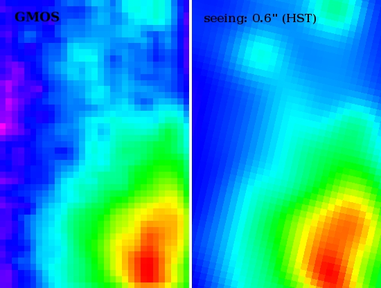
Figure 1: Left: R-band continuum image from GMOS-IFU. Right: HST/ACS (F606W filter) image convolved by a bidimensionsal gaussian corresponding to a seeing FWHM of 0.6 arcsec and binned to the GMOS pixel size of 0.1 arcsec.

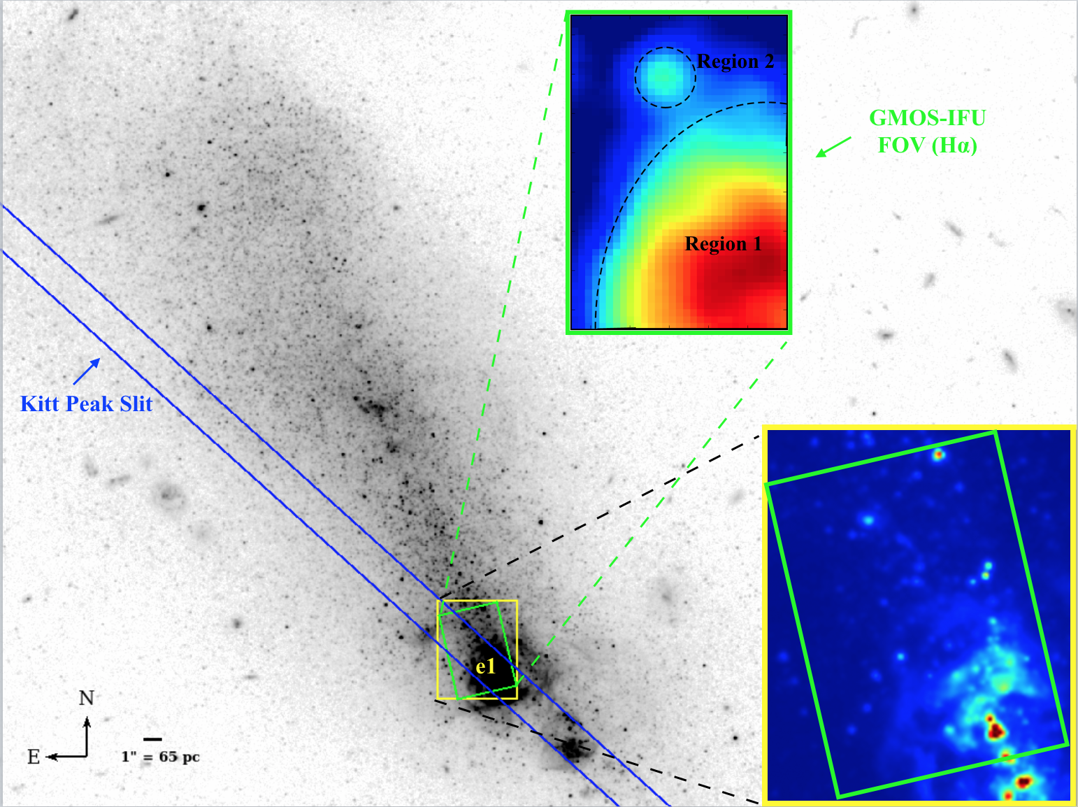
Figure 2: HST/ACS image (0.05 arcsec per pixel) of SBS1415+437 taken in the F606W (V) filter from Aloisi et al. (2005). The small green rectangular box inside the yellow rectangular box shows the GMOS aperture (3.5 $\times$ 5 arcsec²) centered at (RA, Dec) : (214.2559958, 43.50158528). The lower-right inset denotes the zoomed-in version of the small yellow and green boxes. The upper inset is the H$\alpha$ image created from GMOS-IFU data presented here, where we mark principal emission regions as Region 1 and Region 2. The colour scale and stretch of background and inset HST images are set to be different for better visibility. The blue parallel lines represent the long-slit position of spectroscopic observation with Kitt Peak 4m Mayall Telescope, used by Guseva et al. (2003) to study various regions, including "e1" which coincides with our GMOS data. The compass on the bottom-left of the figure shows North and East on the HST image. At the distance of this galaxy, 1 arcsec corresponds to 65 pc.

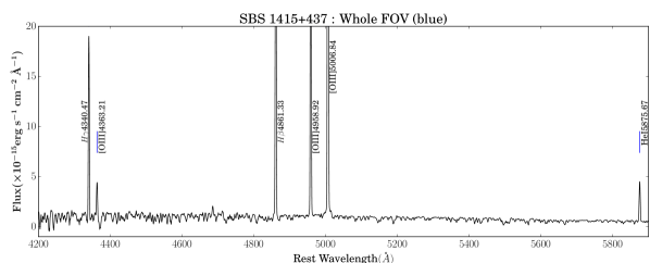
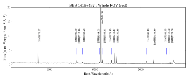
Figure 3: GMOS-IFU integrated spectra of SBS1415+437 integrated over the entire FOV. The principal emission lines are marked as blue lines at their rest wavelengths. The spectra are smoothed using a one-dimensional box kernel with an effective smoothing of 7 pixels.

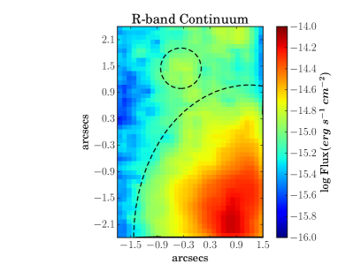
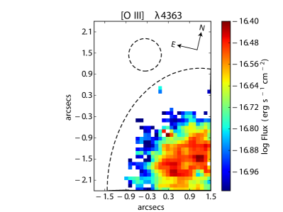
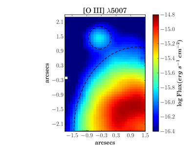
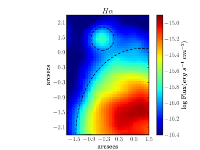
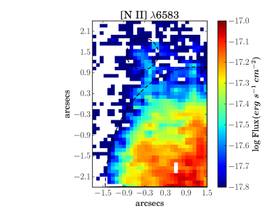
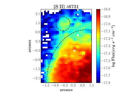
Figure 4: Observed R-band continuum map and the emission line flux maps ([O iii]$\lambda$4363, [O iii]$\lambda$5007, H$\alpha$, [N ii]$\lambda$6583 and [Sii]$\lambda$6731) of SBS 1415+437. The dashed quarter ellipse and circle indicate the H ii regions identified by a relatively higher flux values, and are referred as Region 1 and Region 2, respectively, in the rest of the paper. The spaxels in which emission line fluxes had S/N $<$ 3, are shown in white.

2 Observation & Data Reduction

The target region of SBS1415+437 was observed with GMOS and the IFU unit (GMOS-N IFU; Allington-Smith et al., 2002) at Gemini-North telescope in Hawaii. The observation was taken in one-slit queue-mode in 2012 as a part of GMOS-IFU spectroscopy programme (PI: B James) for seven star-forming galaxies. The field-of-view covered in this mode of observation is 3.5″$\times$ 5″, and is sampled by 750 hexagonal lenslets of projected diameter of 0.2″, of which 250 lenslets are used for background determination (see Table 2 for information on data observation). The blue and red regions of the optical spectrum were observed by using gratings B600+_G5307 and R600+_G5304. A set of standard observations of GCAL flats, CuAr lamp for wavelength calibration and standard star for flux calibration were taken with each grating.

We used the standard GEMINI reduction pipeline written in Image Reduction and Analysis Facility (IRAF) to perform the basic steps of data reduction which included bias subtraction, flat-field-correction, wavelength calibration, sky subtraction, differential atmospheric correction and for conversion of observed spectra into three-dimensional data cubes. We found that the standard pipeline did not give satisfactory results for some procedures, for which we developed and implemented our own code (see Kumari et al., 2017; Kumari et al., 2018). For both data cubes, we chose a spatial-sampling of 0.1″which is suitable to preserve the hexagonal sampling of the GMOS-IFU lenslets. We corrected the data cubes corresponding to the two gratings for a spatial-offset of 0.2″on both spatial-axes, and finally converted them to the row-stacked spectra for further analysis. We estimated the instrumental broadening (Full Width Half Maximum, FWHM $\sim$ 1.7 Å) for both gratings, by fitting a Gaussian profile to several emission lines of the extracted row stacked spectra of the arc lamp. We estimated the seeing FWHM of $\sim$0.6 arcsec by comparing the R-band continuum image from GMOS-IFU with the convolved and binned image of this galaxy obtained from the Hubble Space Telescope (HST) (Figure 1). The original HST Advanced Camera Surveys (ACS) image was taken in the equivalent of the F606W(V) filter and had a resolution of 0.05 arcsec per pixel (program # 9361, PI: Aloisi).

Table 3: Emission line measurements (relative to H$\beta$ = 100) for the integrated spectrum of Region 1 (Quarter Ellipse) (see Section 3.1). Line fluxes ($F_{\lambda}$) are extinction corrected using E(B-V) to calculate $I_{\lambda}$.

Line	$\lambda_{air}$	$F_{\lambda}$ (Region 1)	$I_{\lambda}$ (Region 1)
$H\gamma$	4340.47	$47.15\pm 0.56$	$48.36\pm 1.37$
$[OIII]$	4363.21	$8.87\pm 0.60$	$9.09\pm 0.66$
$H\beta$	4861.33	$100.00\pm 0.47$	$100.00\pm 1.76$
$[OIII]$	4958.92	$119.89\pm 0.80$	$119.40\pm 2.94$
$[OIII]$	5006.84	$356.30\pm 2.29$	$354.03\pm 8.66$
$HeI$	5875.67	$10.72\pm 0.20$	$10.30\pm 0.29$
$[OI]$	6300.3	$2.09\pm 0.06$	$1.98\pm 0.07$
$[SIII]$	6312.1	$1.47\pm 0.05$	$1.39\pm 0.06$
$H\alpha$	6562.8	$303.55\pm 1.62$	$286.00\pm 6.08$
$[NII]$	6583.41	$2.92\pm 0.40$	$2.75\pm 0.38$
$HeI$	6678.15	$2.84\pm 0.05$	$2.67\pm 0.07$
$[SII]$	6716.47	$8.59\pm 0.08$	$8.06\pm 0.18$
$[SII]$	6730.85	$6.14\pm 0.07$	$5.76\pm 0.14$
$[ArIII]$	7135.8	$4.14\pm 0.05$	$3.84\pm 0.09$
$[OII]$	7318.92	$1.64\pm 0.10$	$1.51\pm 0.10$
$[OII]$	7329.66	$1.31\pm 0.09$	$1.22\pm 0.08$
E(B-V)		0.057$\pm$0.005
F(H$\beta$)		117.42 $\pm$ 0.55	141.97 $\pm$ 2.50

Notes: F(H$\beta$) in units of $\times$ 10^-15 erg cm^-2 s^-1

3 Results & Discussion

3.1 Observed and Intrinsic Fluxes

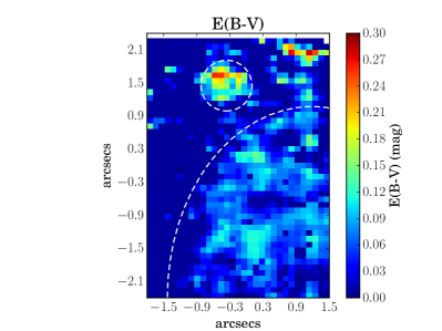
Figure 5: E(B-V) map created assuming the LMC extinction curve. Spaxels with E(B-V) $<$ 0 are set to E(B-V) of the Milky Way foreground along the line-of-sight. The spaxels in which emission line fluxes had S/N $<$ 3, are shown in white. The dashed quarter ellipse and circle indicate Region 1 and Region 2, respectively.

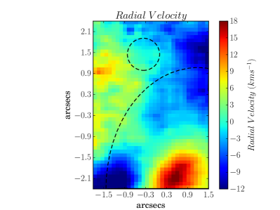
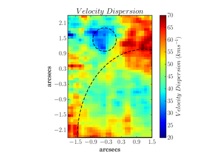
Figure 6: Radial velocity (upper panel) and velocity dispersion (bottom panel) maps of the ionised gas obtained from the H$\alpha$ emission line. Radial velocity is corrected for systemic ($\sim$ 609 km s^-1) and barycentric ($\sim$ $-$6.90 km s^-1) velocities. Velocity dispersion is corrected for instrumental broadening. The dashed quarter ellipse and circle indicate Region 1 and Region 2, respectively.

Figure 2 shows the HST/ACS image of SBS1415+437 taken in the F606W (V) filter from Aloisi et al. (2005). The green rectangular box represents the GMOS aperture (3.5$\arcsec$ $\times$ 5$\arcsec$). The upper-inset shows the H$\alpha$ image obtained from GMOS IFU data where we mark Region 1 and Region 2 selected on the basis of an isophotal H$\alpha$ emission. The blue parallel lines indicate the long-slit position of the Kitt Peak 4m Mayall Telescope observations used in the analysis of Guseva et al. (2003, hereafter G03). Figure 3 shows the GMOS-IFU integrated spectra of the entire FOV in the blue and red parts of the optical spectrum. We have overplotted the principal emission lines at their rest wavelengths in air.

We estimate the emission line fluxes for the recombination and collisionally excited lines within the spectra by fitting Gaussian profiles after subtracting the continuum and absorption features in the spectral region of interest. We give equal weight to flux in each spectral pixel while fitting Gaussians. The fitting uncertainties on the three Gaussian parameters (amplitude, centroid and FWHM) are propagated to estimate the uncertainty in fluxes. These uncertainty estimates are consistent with those calculated from Monte Carlo simulations. We have propagated these estimated uncertainties in the fluxes to other quantities using Monte Carlo simulations in the subsequent analysis.

Figure 4 shows the observed fluxes of R-band continuum, [O iii] $\lambda$4363, [O iii] $\lambda$5007, H$\alpha$, [N ii] $\lambda$6583 and [Sii] $\lambda$6731 over the FOV. We obtained the R-band continuum by integrating the red cube in the wavelength range of 5890–7270 Å  (in the rest wavelength). In all maps, white spaxels correspond to spaxels in which emission lines have S/N < 3. The [O iii] $\lambda$4363 has S/N $>$ 3 for a region extending over 143 $\times$ 143 pc², though all pixels do not show detection (Figure 4, upper-right panel). Note here that we could not detect the [O ii] $\lambda\lambda$3727,3729 doublet in our data because of the low sensitivity of the blue wavelength end of the GMOS-IFU. In all flux maps, there are two distinct regions with elevated fluxes, represented by a quarter-ellipse and a circle, which we refer as Region 1 and Region 2 in subsequent analysis (also see Figure 2). We detect [O iii] $\lambda$4363 in the integrated spectrum of Region 1, but not in Region 2, so analysis involving this emission line is not performed for Region 2. The observed fluxes of the main emission lines in the integrated spectrum of Region 1 are presented in Table 3.

To estimate dust attenuation, we used the attenuation curve of Large Magellanic Cloud (LMC Fitzpatrick, 1999) along with the observed H$\alpha$/H$\beta$ ratio to first estimate the nebular emission line colour excess E(B–V), at an electron temperature and density of 10000 K and 100 cm^-3, respectively (Case B recombination). While mapping E(B-V), we found that some spaxels away from the bright star-forming regions have negative values of E(B–V) which is most likely due to stochastic error and shot noise (Hong et al., 2013). For such spaxels, we forced E(B–V) to that of the Galactic Foreground (0.0077, Schlafly & Finkbeiner, 2011). Figure 5 shows the E(B-V) map of the FOV, which varies between 0.0077–0.30 mag. The increased value of E(B–V) in Region 1 and Region 2 shows that the star-forming regions are dustier than the rest of the FOV. The E(B–V) map obtained was used to deredden the observed flux maps. From the integrated spectrum of Region 1, we obtain a value of E(B–V) = 0.057$\pm$0.005, which lies in the range of values found in the literature for this region (0.08 by Thuan et al. (1999) and 0.00 by G03). The E(B–V) estimated here was used to deredden the observed emission line fluxes of Region 1. The dereddened/intrinsic fluxes for the main emission lines are shown in Table 3.

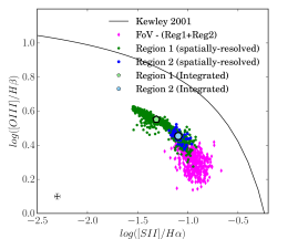
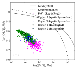
Figure 7: Emission line ratio diagnostic diagrams: [O iii]/H$\beta$ versus [S ii]/H$\alpha$ (left panel), and [O iii]/H$\beta$ versus [N ii]/H$\alpha$ (right panel). Black solid curve and dashed curve represent the theoretical maximum starburst line from Kewley et al. (2001) and Kauffmann et al. (2003), respectively, showing a classification based on excitation/ionisation mechanisms. The line ratios of the two H ii regions are colour-coded as follows: Region 1: green pentagon, Region 2: blue circle. Smaller dark-coloured markers denote the spatially-resolved (spaxel-by-spaxel) line-ratios and the bigger light-coloured markers in black contours denote the line-ratios obtained from the integrated spectrum of the corresponding regions. Magenta coloured markers denote the spatially-resolved line-ratios of the regions of FOV excluding the two H ii regions. The size of error bars varies for line ratios and the median error bars are shown in left corner of each panel.

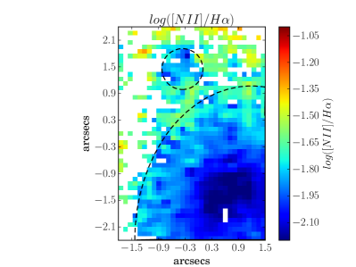
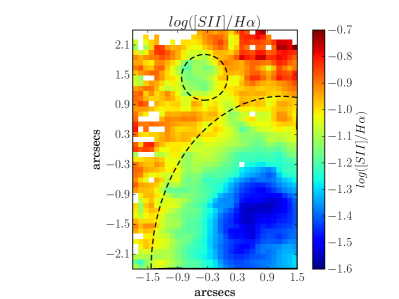
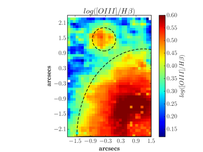
Figure 8: Emission line ratio maps of [N ii] $\lambda$6583/H$\alpha$ (upper-left panel), [S ii] $\lambda\lambda$6717,6731/H$\alpha$ (upper-right panel) and [O iii] $\lambda$5007/H$\beta$ (bottom panel). The dashed quarter ellipse and circle indicate Region 1 and Region 2, respectively. The spaxels in which emission line fluxes had S/N $<$ 3, are shown in white in above line ratio maps.

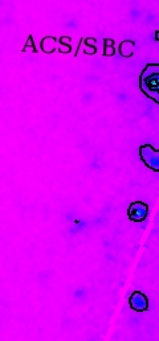
Figure 9: Left panel: ACS/SBC image (0.025″per pixel) of SBS 1415+437 taken in F125LP filter. Right panel: [O iii]/H$\beta$ map created from the GMOS-IFU data. Black contours are generated from the FUV image on the left panel and are overlaid on the emission line ratio map, to trace the relative position of hot O and B stars and the ionised gas.

3.2 Gas Kinematics

Figure 6 shows the maps of radial velocity (upper panel) and velocity dispersion (lower panel) of the H$\alpha$ emission line, which we obtained from the centroid and the FWHM of the Gaussian fit to the emission line. The radial velocity map is corrected for the systemic velocity of 609 kms^-1, and the barycentric velocity of $-$6.9 kms^-1. The velocity dispersion map is corrected for the instrumental broadening of 1.7 Å which corresponds to $\sim$ 78 km s^-1 at the rest-wavelength of the H$\alpha$ emission line.

Figure 6 (upper panel) shows that the radial velocity of the ionised gas in the region of study varies between $\sim$ $-$14 to 19 kms^-1. Thuan et al. (1999) reports a solid body rotation for this BCD across $\sim$ 30″. Though our data clearly shows blueshift and redshift at different locations of the FOV, we do not find a definite axis of rotation. This could be because our FOV is comparatively small (3.5″$\times$ 5″).

Figure 6 (bottom panel) shows that the velocity dispersion of the ionised gas in the region of study varies between $\sim$20–70 kms^-1. Region 1 shows a range of values, whereas Region 2 has a relatively low velocity dispersion. The ionised gas to the north-east of Region 1 and north-west of Region 2 shows the highest values of velocity dispersion.

3.3 Emission line ratio diagnostics

In Figure 7, we show the classical emission line ratio diagnostic diagrams ([O iii]$\lambda$5007/H$\beta$ versus [S ii]$\lambda\lambda$6717,6731/H$\alpha$ (left panel) and [O iii]$\lambda$5007/H$\beta$ versus [N ii]$\lambda$6583/H$\alpha$ (right panel)), which are commonly known as BPT diagrams (Baldwin et al., 1981). In both panels, we show the maximum starburst line also known as the “Kewley line” as the solid black curve, which presents a classification based on ionisation/excitation mechanism. On the [N ii] diagnostic diagram (Figure 7, right panel), the dashed black curve represents the empirical line derived by Kauffmann et al. (2003) using SDSS spectra of 55 757 galaxies. Our spatially-resolved line ratios are shown by blue, green and magenta markers which correspond to the spaxels of Region 1, Region 2 and the rest of the FOV, respectively. We also show the line ratios obtained from the integrated spectra of Region 1 and Region 2 using larger markers. In the [N ii]-BPT diagram, we find that both spatially-resolved and integrated data lie well below and to the left of the Kewley line, as well as the empirical line of Kauffmann et al. (2003), while on the [S ii]-BPT diagram, we find that both spatially-resolved and integrated data lie well below and to the left of the Kewley line. This shows that the ionised gas in the region under study is predominantly ionised by the photons from the massive stars.

Figure 8 shows the line ratio maps of the region under study, which we use to study the ionisation structure of the ionised gas. As expected, we find that the peak of emission shows the lowest values of [N ii] $\lambda$6583/H$\alpha$ (upper-left panel) and [S ii] $\lambda\lambda$6717,6731/H$\alpha$ (upper-right panel), and highest values of [O iii] $\lambda$5007/H$\beta$ (lower panel). This indicates that the more luminous regions (on H$\alpha$ map) have relatively high excitation, which is due to the presence of young and massive stars producing harder ionising radiation. Figure 9 shows a comparison of ACS/Solar Blind Channel (SBC) FUV (far ultra violet) image of SBS 1415+437 in the F125LP filter (program id: JB7H08010, PI: A Aloisi) and the emission line ratio map [O iii]/H$\beta$ created from GMOS data. The contours generated from ACS/SBC image (left panel) are over-plotted on the [O iii]/H$\beta$ map (right panel). We find that there is an offset between the peak of [O iii]/H$\beta$ and the peak of FUV image which traces the young stars, and that the enhancement of [O iii]/H$\beta$ is on the periphery of the stars traced by FUV. This indicates that the enhancement of [O iii]/H$\beta$ ratio has resulted due to the ionisation of gas by hot O and B stars in the surrounding regions. Note here that the peak of H$\alpha$ map is offset by $\sim$ 58 pc with respect to the peak of the R-band continuum indicative of the region containing an older stellar population.

Table 4: Summary of nebular diagnostics, ionic abundances, elemental abundances and abundance ratios obtained from the integrated spectrum (Value $\pm$ Uncertainty), and the spatially-resolved maps (Median $\pm$ Uncertainty) of Region 1. The uncertainty on the median takes into account the correlation between pixels due to resampling in forming data cube.

	Integrated spectrum	Spatially-resolved Map
Parameter	Value $\pm$ Uncertainty	Median $\pm$ Uncertainty
Te([O iii]) ($\times$ 104)	1.71 $\pm$ 0.07	1.72 $\pm$ 0.02
Te([O ii]) ($\times$ 104)	1.59 $\pm$ 0.05	1.53 $\pm$ 0.02
Te([N ii]) ($\times$ 104)	1.42 $\pm$ 0.03	1.42 $\pm$ 0.01
Te([S iii]) ($\times$ 104)	1.71 $\pm$ 0.09	1.72 $\pm$ 0.03
Ne([SII]) (cm-3)	$<$ 50	50 $\pm$ 9
12 + log(O+/H+)	7.15 $\pm$ 0.06	7.21 $\pm$ 0.03
12 + log(O2+/H+)	7.46 $\pm$ 0.04	7.48 $\pm$ 0.01
12+ log(O/H)	7.63 $\pm$ 0.03	7.67 $\pm$ 0.02
12 + log(N+/H+)	5.41 $\pm$ 0.05	5.39 $\pm$ 0.01
ICF(N+)	3.03 $\pm$ 0.47	2.79 $\pm$ 0.09
12 + log(N/H)	5.89 $\pm$ 0.08	5.84 $\pm$ 0.02
N/O	-1.74 $\pm$ 0.09	-1.82 $\pm$ 0.02
S+/H+ ($\times$ 107)	1.31 $\pm$ 0.06	1.27 $\pm$ 0.06
S2+/H+ ($\times$ 107)	4.95 $\pm$ 0.69	5.02 $\pm$ 0.33
ICF (S+ + S2+)	1.10 $\pm$ 0.02	1.08 $\pm$ 0.01
12 + log(S/H)	5.84 $\pm$ 0.05	5.83 $\pm$ 0.02
log(S/O)	-1.79 $\pm$ 0.06	-1.83 $\pm$ 0.02
Ne2+/H+ ($\times$ 105)	0.49 $\pm$ 0.08	0.55 $\pm$ 0.03
ICF (Ne2+)	1.10 $\pm$ 0.01	1.11 $\pm$ 0.03
12 + log(Ne/H)	6.73 $\pm$ 0.07	6.80 $\pm$ 0.02
log(Ne/O)	-0.90 $\pm$ 0.08	-0.90 $\pm$ 0.02
Ar2+/H+ ($\times$ 107)	1.23 $\pm$ 0.09	1.23 $\pm$ 0.03
ICF (Ar2+)	1.15 $\pm$ 0.01	1.16 $\pm$ 0.01
12 + log(Ar/H)	5.15 $\pm$ 0.03	5.16 $\pm$ 0.01
log(Ar/O)	-2.48 $\pm$ 0.04	-2.50 $\pm$ 0.01

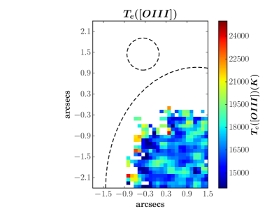
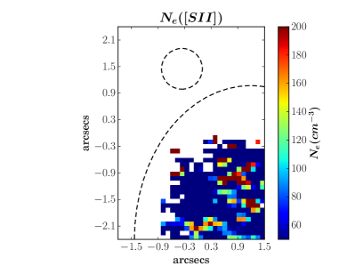
Figure 10: Upper panel: Map of electron temperature of high-ionisation zone (T_e([O iii])). Lower panel: Electron density (N_e([S ii])) map obtained from the [S ii] doublet ratio and T_e([O iii]) map. The dashed quarter ellipse indicates Region 1. The spaxels in which emission line fluxes had S/N $<$ 3, are shown in white. Single pixel features or few-pixel features should be interpreted with caution since the seeing FWHM (0.6 arcsec) extends over 6 pixels.

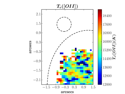
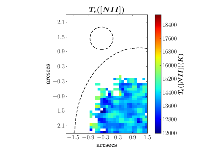
Figure 11: Temperature maps of low- and intermediate ionisation zones: T_e([O ii]) (upper-left panel), T_e([N ii]) (upper-right panel) and T_e([S iii]) (lower panel). The dashed quarter ellipse and circle indicate Region 1 and Region 2. The spaxels in which emission line fluxes had S/N $<$ 3, are shown in white.

3.4 Electron temperature and density

An H ii region is a complex structure. In the following analysis, the thermal structure of a H ii region is assumed to be approximated by a three-zone model (Garnett, 1992). This model consists of a high-ionisation zone, a low-ionisation zone and an intermediate-ionisation zone. The innermost high-ionisation zone corresponds to species such as O²⁺, Ne²⁺, Fe²⁺, He⁺ and Ar³⁺. The outermost low-ionisation zone corresponds to species such as O⁺, N⁺ and S⁺. The region between the two is the intermediate-ionisation zone and corresponds to species such as Ar²⁺ and S²⁺. The electron temperature of each zone can be approximated from the temperature of the species related to that zone.

To estimate electron temperature T_e([O iii]), we use the dereddened [O iii] line ratio, [O iii] ($\lambda$5007 $+\lambda$4959)/[O iii]$\lambda$4363 and the calibration from Pérez-Montero (2017, hereafter P17), which is derived assuming a five-level atom, using collision strengths from Aggarwal & Keenan (1999). Figure 10 (upper panel) shows the derived T_e([O iii]) map. From the integrated spectrum of Region 1, we find T_e([O iii]) = 17100 $\pm$ 700 K, in agreement with the value found by G03  (16490 $\pm$ 140 K).

To derive the electron density N_e, we use [S ii] doublet ratio and T_e([O iii]) derived above, along with the theoretical curves of the [S ii] doublet ratio versus N_e at given temperatures. Figure 10 (lower panel) shows the N_e map, where we find that majority of the spaxels have N_e $<$ 50 cm^-3, indicating that the region under study lies in the low-density regime. From the integrated spectrum of Region 1, we find N_e $<$ 50 cm^-3 which is in agreement with the value (60 $\pm$ 30 cm^-3) found by G03.

The temperature of low-ionisation zone T_e([O ii]) is estimated by using N_e and T_e calculated above and the density-dependent calibration given in P17. The T_e([O ii]) map (Figure 11, upper-left panel) shows a mean and standard deviation of $\sim$15000 K and $\sim$1600 K, respectively. We calculated T_e([O ii]) $\sim$15900 $\pm$ 500 for the integrated spectrum of Region 1, which is higher than the value found by G03  (14430 $\pm$ 110 K). The main difference is that G03  have used the expression from Izotov et al. (1994), which is independent of density. Using their expression, we find the value to be $\sim$14700 $\pm$ 300 K for the integrated spectrum Region 1, which is in good agreement with their value (G03). The electron density should be taken into account in determining T_e([O ii]) because of only a weak correlation between T_e([O ii]) and T_e([O iii]) (Hägele et al., 2006, 2008; López-Hernández et al., 2013).

We map T_e([N ii]) (Figure 11, upper-right panel) by using the T_e([O iii]) map in the calibration of Pérez-Montero & Contini (2009), which is based on photoionisation models. The map shows a variation of 11900–16300 K. For the integrated of spectrum Region 1, we followed same procedure involving the T_e([O iii]) estimated above and calculated T_e([N ii]) = 14200 $\pm$ 300 K.

Though both T_e([O ii]) and T_e([N ii]) correspond to temperatures of low-ionisation zones, their maps show different structure. This is because the recipe used to obtain T_e([O ii]) involves the use of N_e([S ii]), which results in similar structures in T_e([O ii]) and N_e([S ii]) maps, whereas T_e([N ii]) is directly obtained from T_e([O iii]). For the integrated spectrum of Region 1 as well, we find that T_e([N ii]) is slightly lower than T_e([O ii]), even though both ions lie in the same excitation zone of a nebula. Note here that photoionisation models predicted a higher T_e([O ii]) than T_e([N ii]) for the brightest knot BCD Mrk 209 (Pérez-Montero & Díaz, 2007). It is possible that the temperature of the two ions T_e([O ii]) and T_e([N ii]) might not be the same even if originating from the same ionisation zone.

We map the temperature of the intermediate-ionization zone T_e([S iii]) by using the empirical fitting between T_e([O iii]) and T_e([S iii]) given by Hägele et al. (2006), which has a calibration uncertainty of the order of 12%. The T_e([S iii]) map (Figure 11, lower panel) shows a mean and standard deviation of 17000 K and 2000 K, respectively. Following the same procedure for the integrated spectrum of Region 1, we estimated T_e([S iii]) = 17100$\pm$900 K, which is higher than reported by G03 (15380 $\pm$ 110 K), but is in agreement with their value if we consider the large calibration uncertainty from Hägele et al. (2006). G03  have followed the procedure of Garnett (1992), who assumed that T_e([S iii]) = T_e([Ar iii]) and estimated T_e([Ar iii]) from T_e([O iii]). Using their recipe, we get a value of T_e([S iii]) = 15900 $\pm$ 600 which is in good agreement with G03.

Table 4 summarizes the above results for the integrated spectrum of Region 1 and the spatially-resolved data. In this table, we report median and the uncertainty on the median of the values on the entire map and take into account the correlation between pixels due to resampling in forming data cube.

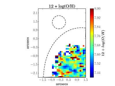
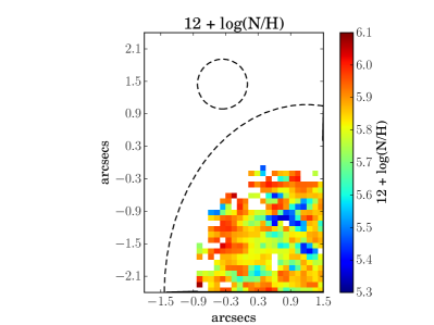
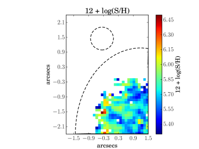
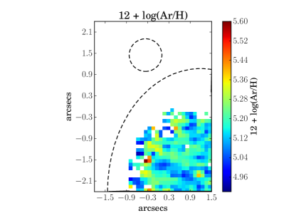
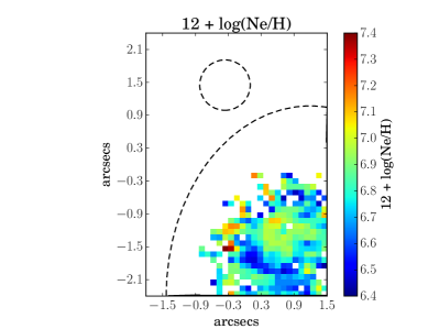
Figure 12: Maps of elemental abundances of oxygen, nitrogen, sulphur, argon and neon. They are obtained by first estimating the ionic abundances and then applying the ICF on a pixel-by-pixel basis. The dashed quarter ellipse and circle indicate Region 1 and Region 2, respectively. Single pixel features or few-pixel features should be interpreted with caution since the seeing FWHM (0.6 arcsec) extends over 6 pixels. The median uncertainties on elemental abundance maps of oxygen, nitrogen, sulphur, argon and neon are 0.08 dex, 0.19 dex, 0.3 dex, 0.3 dex and 0.3 dex, respectively, as estimated from the corresponding uncertainty maps given in Figure 21.

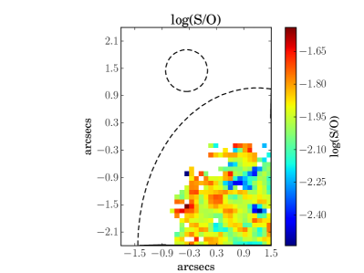
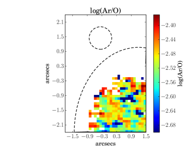
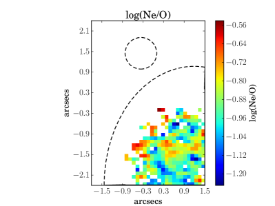
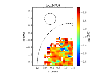
Figure 13: Abundance ratios of S/O, Ar/O, Ne/O and N/O. The dashed quarter ellipse and circle indicate Region 1 and Region 2, respectively. Single pixel feature or few-pixel features should be interpreted with caution since the seeing FWHM (0.6 arcsec) extends over 6 pixels. The median uncertainties on maps of S/O, Ar/O, Ne/O and N/O are 0.3 dex, 0.3 dex, 0.3 dex and 0.2, respectively, as estimated from the corresponding uncertainty maps given in Figure 22.

3.5 Chemical Abundances

3.5.1 Ionic and Elemental Abundance

For both spatially-resolved data and the integrated spectrum of Region 1, we estimate the ionic abundances (O⁺/H⁺, O²⁺/H⁺, N⁺/H⁺, S⁺/H⁺, S²⁺/H⁺, Ne²⁺/H⁺ and Ar²⁺/H⁺). We calculate the corresponding ionisation correction factor (ICF) for each elemental species. Different ICF recipes exist which may or may not depend on metallicity, depending on the assumptions of the photoionisation models used for deriving ICF expressions (see e.g. Izotov et al., 2006; Pérez-Montero et al., 2007). Such details of the ICF prescription for each ionic species are described below. The ICFs are combined with ionic abundances to estimate the elemental abundances of oxygen, nitrogen, sulphur, neon and argon. Table 4 presents the ionic and elemental abundances obtained from the integrated spectrum of Region 1 and also the spatially-resolved maps for which we give the median and the uncertainty of all valid data. We find that the inferred values of the quantities for the integrated spectrum and spatially-resolved data are in reasonable agreement with each other. In the following points, we describe the methodology used to derive the chemical abundance maps shown in Figure 12. Corresponding uncertainty maps are presented in Figure 21.

• Oxygen abundance: The metallicity of the ionised gas is expressed as the oxygen abundance as oxygen is the most prominent heavy element observed in the optical spectrum. The total oxygen abundance (12 + log(O/H)) is calculated from the sum of O⁺/H⁺ and O⁺⁺/H⁺. Generally, O⁺/H⁺ is estimated from the oxygen doublets of [O ii] $\lambda\lambda$3727,3729. However, we could not detect these doublets in our data due to the low sensitivity of GMOS-N IFU in the blue end of the optical spectrum. Instead, we use [O ii] $\lambda\lambda$7320,7330 to estimate O${}^{+}/H^{+}$ at the low-ionisation zone temperature T_e([O ii]) by employing the formulation of Kniazev et al. (2003). We estimated O⁺⁺/H⁺ using the [O iii] $\lambda\lambda$4959, 5007 at the high ionisation zone temperature T_e([O iii]) using the formulation of P17. Finally we combined O⁺/H⁺ and O⁺⁺/H⁺, and obtained the total metallicity. Map is shown in Figure 12 (upper-left panel).

• Nitrogen abundance: [N ii] $\lambda$6548 is not detected with S/N $>$ 3, but [N ii] $\lambda$6583 is detected at sufficient S/N. Assuming an intrinsic emission line ratio between the two nitrogen lines [N ii] $\lambda$6548 = (1/2.9)[N ii] $\lambda$6583, we estimated the dereddened [N ii] $\lambda$6548 from the dereddened flux of [N ii]$\lambda$6583. Using the dereddened flux of [N ii] lines and T_e([N ii]) estimated in Section 3.4, we employed the formula given in P17  to map 12 + log(N⁺/H⁺). We estimated ICF(N⁺) from the abundance maps of total oxygen and singly-ionised oxygen, and finally mapped 12 + log(N/H) (Figure 12, upper-right panel).

• Sulphur abundance: We estimated singly-ionised sulphur abundance (S⁺/H⁺) by using the dereddened [S ii] $\lambda\lambda$6717, 6731 and T_e([O ii]). The auroral line [S iii] $\lambda$6312 was used along with T_e([S iii]) to estimate S²⁺/H⁺. All of these estimates were derived by using the corresponding expressions given in P17. We estimated ICF(S⁺ + S²⁺) using the classical formula from Stasińska (1978), but using $\alpha$ = 3.27 derived by Dors et al. (2016). We finally combined ionic abundance with the ICF correction to derive the elemental sulphur abundance, 12 + log(S/H). Corresponding map is shown in Figure 12 (middle-left panel).

• Neon abundance: We estimated doubly-ionised neon abundance (Ne²⁺/H⁺) by using the dereddened [Ne iii] $\lambda$3869 and T_e([O iii]), and derived ICF(Ne²⁺) using the expressions from Pérez-Montero et al. (2007), which is independent of metallicity. Combining the ionic-abundance with the ICF, we derived the elemental neon abundance, 12 + log(Ne/H). Map is shown in Figure 12 (lower panel).

• Argon abundance: We estimated doubly-ionised argon abundance (Ar²⁺/H⁺) by using the dereddened [Ar iii] $\lambda$7135 and T_e([S iii]) the temperature of intermediate-ionisation zone, in the expression given in P17. We estimated the metallicity-independent ICF(Ar²⁺) using expression given in Pérez-Montero et al. (2007) to derive the elemental argon abundance, 12 + log(Ar/H). Map is shown in Figure 12 (middle-right panel).

The abundance maps of 12 + log(O/H) and 12 + log(N/H) shows relatively high and low values, respectively in the north-east of the peak H$\alpha$ flux exactly at the same location where we find high electron density (Figure 10, lower panel). To check this, we estimated electron densities from the integrated spectra of two different regions within this over-density region. Though their electron densities are high, the associated uncertainties are also large, which indicates that the region may well have the same electron density as the majority of the pixels, i.e. N_e $<$ 50 cm^-3. So we suspect that the abundance patterns on the maps of 12 + log(O/H) and 12 + log(N/H) may not be real variations.

Our derived values of 12 + log(O/H), 12 + log(O²⁺/H⁺), 12 + log(N⁺/H⁺) and Ne²⁺/H⁺ are in excellent agreement with those obtained by G03. However, the values of 12 + log(O⁺/H⁺), S⁺/H⁺, S²⁺/H⁺ and Ar²⁺/H⁺ do not agree with those from G03, since these abundance estimates depend on the low-ionisation zone temperature (T_e ([O ii])) and the intermediate zone temperature (T_e ([S iii])), and these temperature estimates in our work are different from those obtained by G03  for the reasons described in section 3.4.

In the above analysis, our derived ICFs do not match those of G03. As such, we estimated the ICFs for data from G03 using our adopted recipes for ICF calculation, which now exactly match our derived ICFs. The total elemental abundances of nitrogen, sulphur, neon and argon do not match those derived from G03 because of the following two differences: firstly the ionic abundances in the two works are different as a result of the different electron temperatures, secondly different ICF prescriptions have been used in the two works. This results in obvious differences in the abundance ratios between our work and G03. In addition to the ICF and ionic abundances, difference in ionic and elemental abundances might also be due to spatial effects since the GMOS-IFU FOV does not coincide exactly with the long-slit of G03.

3.5.2 Abundance Ratios

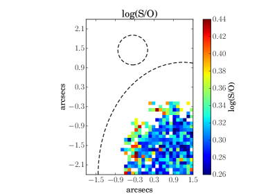
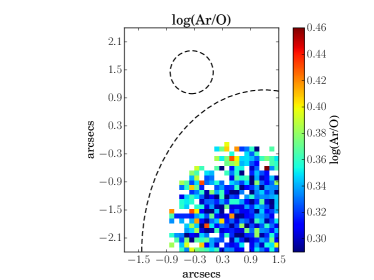
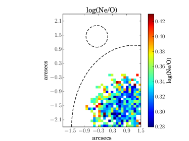
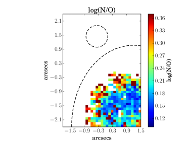
Figure 22: Uncertainty maps for the abundance ratio maps presented in Figure 16.

Figure 13 shows the maps of abundance ratios, while corresponding uncertainty maps are presented in Figure 22. We find an abundance pattern in the north-east region in the maps of S/O, Ar/O and N/O similar to that of the electron density map. Hence, these may not be real as discussed in Section 3.5.1. The abundance ratios for the integrated spectrum and spatially-resolved maps of Region 1 agree with each other within error bars as tabulated in Table 4. Our abundance ratio estimates are systematically lower than those of a sample of 40 BCDs analysed by Izotov & Thuan (1999). However, such low values have been reported in the IFU studies of BCDs. One such BCD is the interaction-induced starburst UM 462 (James et al., 2010) where abundance ratios of N/O, S/O and Ar/O are found to be in agreement with SBS 1415+437 from our study. Likewise, the values of N/O, Ne/O and Ar/O in our BCD are in agreement with those of the main body of another metal-poor BCD Tol 65 (Lagos et al., 2016) where tidal interaction has also been proposed. Though there have been no study reporting the existence of a companion or an interaction-induced starburst in the current BCD under study SBS 1415+437, the comet-shaped structure of this BCD might be indicative of tidal interaction of this galaxy with the local intergalactic environment.

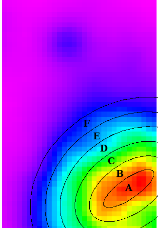
Figure 14: H$\alpha$ flux map is used to separate the H ii region into six equally-spaced segments (A, B, C, D, E, F) such that each of them have similar overall flux within each annulus. These annuli are used for the chemical inhomogeneity investigation described in Section 3.5.3. Please see location of Region 1 in Figure 2.

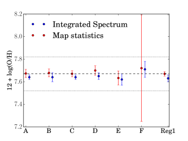
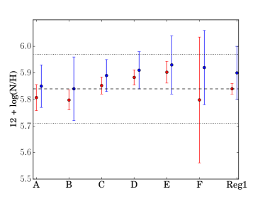
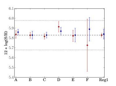
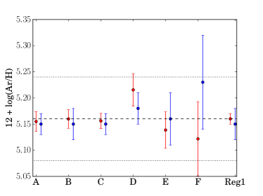
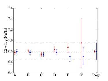
Figure 15: Variation of elemental abundances across Region 1. In all panels, red points with vertical bars correspond to the median of data and the associated uncertainty within annuli A, B, C, D, E, F (shown in Figure 14) of a given chemical abundance map. The error bar corresponding to annulus F is large because of the paucity of data points in this annulus. Blue points are the observables derived from the integrated spectra of each annulus. We also present the corresponding values of entire Region 1 (marked as “Reg1"). The black dashed line corresponds to the median of all data on an abundance map. The dotted black lines indicate the $\pm 1\sigma$ as determined from the standard deviation of all valid data in a map.

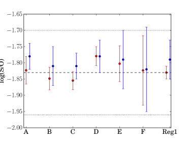
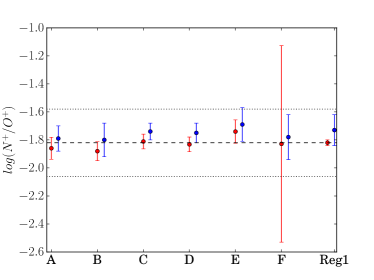
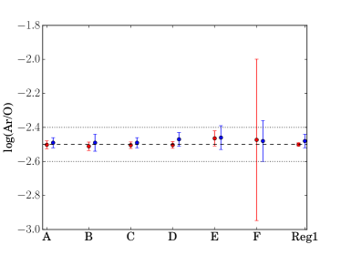
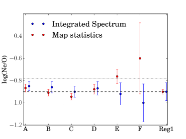
Figure 16: Variation of abundance ratios across Region 1 - see caption of figure 15 for details on legends.

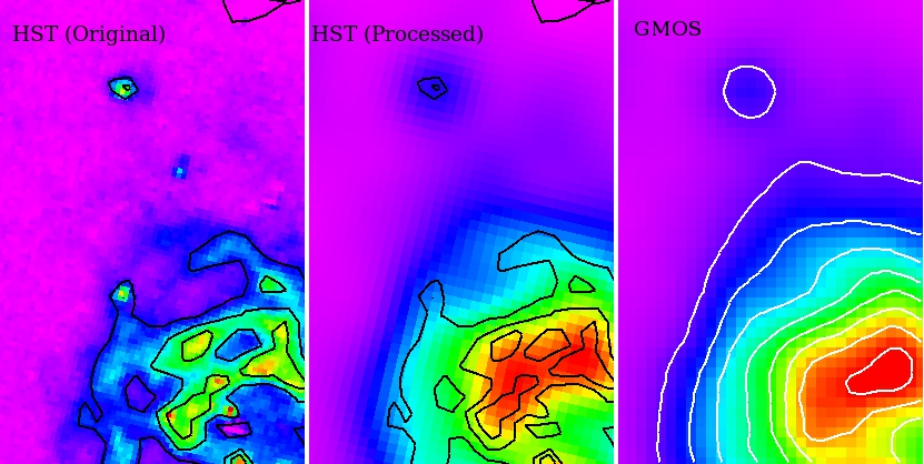
Figure 17: Left: HST continuum subtracted image in F658N filter with pixel sampling of 0.05 arcsec. Middle: HST continuum subtracted image, convolved to the FWHM seeing of 0.6 arcsec and binned to 0.1 arcsec per pixel. The black contours on this panel are generated on the original HST image shown on the left panel. Right: GMOS H$\alpha$ image, where the white contours are generated on this image itself. Comparison of the three images shows that the region under study hosts multiple H ii regions, whose structures are smoothed out in the GMOS image due to seeing lowering the resolution of GMOS compared to HST.

3.5.3 Variation of abundances

The high-resolution HST image shows distinct structure throughout the region of our study (Figure 2). However, the observed H$\alpha$ emission line flux map of Region 1 shows approximately an elliptical distribution (Figure 4). No elliptical distribution is obvious in any abundance maps (Figure 12) or abundance ratio maps (Figure 13), though we note that an over-density is observed in Ne abundance map (Figure 12, bottom panel) in the region north-east of the peak of H$\alpha$ emission. In this Section, we explore the small scale abundance variation to investigate how well-mixed the gas is within the region of study.

We perform this analysis via three different methods, though we show results from only two methods. The first two methods are based on the segmentation of Region 1 in six elliptical annuli of equal widths selected on the basis of the H$\alpha$ flux distribution such that each of the annuli have roughly similar levels of flux within a given annulus. The position of the chosen elliptical annuli are shown in Figure 14, and are marked as A, B, C, D, E and F. In the first method, we estimated abundances and abundance ratios from the emission line fluxes from the integrated spectra within each annulus, which are reported in Table 6. In the second method, we estimate abundances and abundance ratios within each annulus from the spaxel maps instead of integrated spectra. We study the variation of estimates from the two methods from one annulus to another as described later. In the third method, we simply study the variation of abundances in a pixel with respect to its physical distance from the pixel of peak H$\alpha$ flux (i.e. radial distance in elliptical coordinates). This last method was performed to check if our method of segmentation could affect any observed trend.

Figures 15 and 16 show the variation of elemental abundances and abundance ratios from one elliptical annulus to another. The observables from the integrated spectra of each annulus are shown as blue dots. For all maps of abundances and abundance ratios, we estimate median and uncertainty on the median within each annulus, and are shown as red dots and vertical bars, respectively. The uncertainties on the median values for each sample point take into account the spatial correlation between adjacent spaxels arising from the resampling used in generating the data cubes. The overall average level of the correlation was estimated using an autocorrelation analysis of selected regions from the spaxel map after first removing larger scale gradients. In practice this provides an estimate of the factor (in this case $\approx 4$) by which the number of apparently independent spaxels in each elliptical annulus region should be reduced to allow for the induced spatial correlation. The abundance and abundance ratios of region 1 are also shown on the panels in Figures 15 and 16, as estimated from the integrated spectrum (blue dots) and the maps (red dots) for a better visual comparison, and should not be considered for abundance variation analysis. In each panel, the dashed black horizontal line indicates the median ($\mu$) of the abundances or abundance ratio distribution of entire maps, while the two dotted black horizontal lines indicate $\mu$ $\pm$ $\sigma$, where $\sigma$ denoted the standard deviation of entire maps.

Inspecting all panels in Figure 15 and 16, we find that the integrated spectra values and mapped values in each annulus are in reasonable agreement with each other. Results of annulus F should be interpreted with caution where uncertainties on each observable are comparatively large because of a few valid data points ($\sim$ 2–3 depending on the map) in this annulus (see maps in Figures 12 and 13). Though results of annulus F are not particularly informative, we have included them in our analysis as we do not wish to discard any detection.

No variation is found in 12 + log(O/H). There appears to be a variation in abundances of elements (other than O) and abundance ratios around annuli C and D, though these variations are $<$ 0.1 dex for each observable. Given that there exists a region of over-density in the Ne abundance map (Figure 12), it is possible that the physical conditions are different within the region of study and is supported by the HST image which shows structures throughout this region. Figure 17 shows a comparison of H$\alpha$ images obtained with the GMOS-IFU and HST (F658N). The corresponding continuum image (taken in the F606W filter of HST) was scaled and subtracted from the narrow-band F658N image, to obtain the continuum-subtracted H$\alpha$ image (Figure 17, left panel). The overlaid black contours are generated from this original HST image, showing resolvable structure. To compare the HST image directly with the GMOS H$\alpha$ image, we convolved it to FWHM seeing of 0.6 arcsec and rebinned to 0.1 arcsec per pixel. The resultant smoothed image (Figure 17, middle panel) has the black contours generated from the original HST image overlaid for comparison. The processed HST image is remarkably similar to the GMOS H$\alpha$ image (Figure 17, right panel), whose contours (white curves) also show a smooth variation of flux.

Since the region under study appears to host multiple H ii regions, we infer that the absence of radial variation is probably because of the effects of seeing and that a considerable number of pixels with lower abundances in annuli A, B and C have suppressed signatures of over-abundance should they exist. This experiment shows that such segmentation analysis may not be a good tool to find localised abundance variation, which results in averaging out such local effects.

We also performed a Lillefors test of normality for testing homogeneity on the maps of abundances and abundance ratios, which was inconclusive. Peforming the Lillefors test on the abundance and abundance ratio maps normalised by their error maps was also inconclusive. For example, the p-value of Lillefors test was greater than 0.05 for Ne abundance map indicating chemical homogeneity in spite of the map apparently showing some chemical inhomogeneity. Hence, we conclude that tests of chemical inhomogeneity must account for both the spatial information as well as the spaxel error. The current analysis also shows the power of IFS with good spatial-sampling, without which over-abundance in the Ne abundance map would only have appeared as noise. Furthermore, we need to consider the effects of seeing which tends to wash out small spatial scale variation in the abundance maps.

3.6 Stellar Properties

3.6.1 Age of stellar population

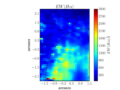
Figure 18: Map of the equivalent width of H$\alpha$ (in Å). The dashed quarter ellipse and circle indicate Region 1 and Region 2, respectively.

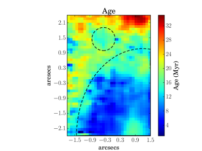
Figure 19: Age map in Myr estimated from Starburst99 models at a constant metallicity of Z = 0.1 Z_⊙ (mean of the metallicity map in Figure 12, upper-left panel). The dashed quarter ellipse and circle indicate Region 1 and Region 2, respectively.

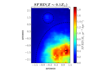
Figure 20: SFRD map assuming a constant metallicity of Z = 0.1 Z_⊙ (mean of the metallicity map in Figure 12, upper-left panel). The dashed quarter ellipse and circle indicate Region 1 and Region 2, respectively.

The integrated spectrum of the FOV (Figure 3) show Balmer emission lines indicating the presence of young, hot and massive O and B stars embedded in gas, while we do not find any Balmer absorption lines showing that the region is mostly composed of younger stellar population. No Wolf-Rayet features are found in the integrated or spatially-resolved spectra of SBS 1415+437, in agreement with the results of López-Sánchez & Esteban (2010).

For age-dating the current ionising population, we first map the equivalent width (EW) of the H$\alpha$ recombination line (Figure 18).This map shows a mean of $\sim$696 Å and standard deviation of $\sim$440  Å. From the integrated spectrum of Region 1, we find an equivalent width of $\sim$940 $\pm$ 10 Å, which is in reasonable agreement with the value found by G03 (997.9 $\pm$ 1.7 Å).

Next, we calculate the EW(H$\alpha$) from the evolutionary synthesis models of starburst99. Note here that the starburst99 models are used here considering that an individual spaxel might constitute an independent H ii region on the basis of the following argument. H$\alpha$ flux map (Figure 4, middle-right panel) shows a variation of 4.0$\times$10^-17 to 1.2$\times$10^-15 erg s^-1 cm^-2, which corresponds to luminosities varying between 8.9$\times$10³⁵ and 2.7$\times$10³⁷ erg s^-1 and ionising photons varying between 6.5$\times$10⁴⁷ and 2.0$\times$10⁴⁹ photons s^-1. The ionising photons on a spaxel-by-spaxel basis lie within the range of ionising photons emitted by individual O and B stars, i.e. 10⁴⁶ – 5$\times$10⁴⁹ photons s^-1 for dwarfs and 4$\times$ 10⁴⁷ – 8$\times$10⁴⁹ photons s^-1 for supergiants (Sternberg et al., 2003). This shows that each spaxel might host O and B stars leading to H ii regions, though we can not discard the effects of a stochastic sampling of the initial mass function at such small spatial scales. The parameters and assumptions for running these models are described in detail in Kumari et al. (2017), which include the assumptions of instantaneous starburst, Salpeter intial mass function, Geneva tracks with stellar rotation and expanding atmosphere models. The only difference here is on the assumption of metallicity, which is the mean of the metallicity map (Figure 12, upper-left panel), i.e. Z = 0.1Z_⊙. Note here that instead of assuming a constant metallicity for the entire FOV, we could use the metallicity map where metallicity varies from spaxel to spaxel. Howeover, the minimum metallicity of the spectra output by Starburst99 is 0.05Z_⊙, whereas our metallicity map shows values $<$ 0.05Z_⊙. Moreover, the metallicity grid used by Starburst99 is far too coarse to correctly reflect the pixel-to-pixel variation seen in our maps. Hence, with the current set of models, it is not possible to create an age map varying as a function of metallicity. By comparing the modelled EW from the evolutionary synthesis models with the observed EW(H$\alpha$), we obtain the age map (Figure 19) which shows a mean and standard deviation of 15 Myr and 6 Myr, respectively. We find the age of $\sim$ 10 Myr for Region 1 obtained from its integrated spectrum. Our results are in reasonable agreement with that of Thuan et al. (1999), who reports the presence of young stellar population ($\sim$ 5 Myr) along with stars as old as 100 Myr in Region 1. G03  estimated an age of 4 Myr for Region 1 from the galactic evolution code PEGASE, which is lower than our value of $\sim$ 10 Myr for two reasons. Firstly the metallicity assumed by G03  is 0.05 Z_⊙ compared to our metallicity assumption of 0.1 Z_⊙. Secondly, our modelling does not take into account nebular continuum or dust-extinction which will lead to systematic uncertainties in the estimated age (Cantin et al., 2010; Pérez-Montero & Díaz, 2007). Note also that Starburst99 does not take into account the binary population, even though $\sim$ 50% of stars are found in binaries. Ignoring the binary population is another source of systematic uncertainty in the determined age. These age estimates should be further interpreted with caution as suggested by Aloisi et al. (2005), who report the presence of stars older than $\sim$ 1.3 Gyr (e.g. red giant branch stars) via a photometric analysis involving colour-magnitude diagrams.

3.6.2 Star Formation Rate

We estimated the star-formation rate (SFR) from the dereddened H$\alpha$ luminosity assuming solar and sub-solar metallicity by using the recipes of Ly et al. (2016) and Kennicutt (1998), respectively assuming a Chabrier IMF. We normalise the SFR map by the area of each pixel to obtain the SFR density (SFRD) map. The SFRD map created assuming sub-solar metallicity (Figure 20) shows a variation of 0.03–1.89 M_⊙ yr^-1 kpc^-2. The SFRD map created assuming solar metallicity shows a variation of 0.06–3.79 M_⊙ yr^-1 kpc^-2 and has the same appearance as the map at sub-solar metallicity. SFR values on pixel-by-pixel basis should be interpreted with caution because of the failure of SFR recipes due to the stochastic sampling of the IMF at such small spatial scales. For Region 1, we find a SFR of $\sim$ 22.0 $\pm$ 0.3 $\times$ 10^-3 M_⊙ yr^-1 assuming metallicity of 12 + log(O/H) = 7.63 , and $\sim$ 44.9 $\pm$ 0.5 $\times$ 10^-3 M_⊙ yr^-1 assuming solar metallicity. For Region 1, we estimate a SFRD $\sim$ 0.7 M_⊙ yr^-1 kpc^-2 from our data assuming a metallicity of 12+log(O/H) = 7.63. For comparison, if we were to use the MMT spectroscopic observation of Thuan et al. (1999) extracted over a region of 1.5 arcsec $\times$ 5 arcsec, we estimate a SFRD $\sim$ 0.5 M_⊙ yr^-1 kpc^-2 assuming 12 + log(O/H) = 7.60 (Thuan et al., 1999). Our value of SFRD agrees with that of Thuan et al. (1999) within a factor of 2. From the H$\alpha$ flux value of G03 , we estimate a SFRD $\sim$ 0.17 M_⊙ yr^-1 kpc^-2 assuming 12 + log(O/H) = 7.61 (G03) over a region of 2 arcsec $\times$ 4.6 arcsec. The low value of SFRD obtained from the data of G03  is due to their estimate of c(H$\beta$) = 0.00, which results in a lower value of dereddened H$\alpha$ flux. It is also possible that the GMOS-FOV covers brighter star-forming regions than the long-slit data of G03.

4 Summary & Conclusion

Using GMOS-N IFS data, we carried out a spatially-resolved analysis of the ionised gas in a star-forming region within the BCD SBS 1415+437 at scales of $\sim$6.5 pc. What follows is a summary of our main results.

1. The radial velocity of the ionised gas varies between $-$12 to 18 km s^-1, with no particular axis of rotation in the central region. The velocity dispersion varies between 20–70 km s^-1. The gas is predominantly photoionised as inferred from the emission line ratio diagnostic diagrams.

2. The IFS data allows us to map the weak auroral line [O iii] $\lambda$4363 across a region of 143 $\times$ 143 pc² thereby enabling us to map the electron temperature T_e([O iii]) and density N_e([S ii]) in this region. This allows us to use the direct T_e-method to map the ionic and elemental abundances of various elements.

3. We map the ionic and elemental abundances of O, N, Ne, Ar and S, and also the abundance ratios, N/O, Ne/O, S/O and Ar/O. We also estimate these observables from the integrated spectrum of the main emission region (Region 1), which are in reasonable agreement with the median of corresponding values in the maps. The oxygen abundance from our IFS data is in agreement with that obtained from the long-slit spectroscopy, i.e. 12 + log(O/H) = 7.63 $\pm$ 0.03.

4. The age map of the region under study shows a mean and standard deviation of 15 Myr and 6Myr, respectively, as inferred from a comparison of the EW(H$\alpha$) map to the values determined from the starburst99 models at a uniform metallicity of 0.1 Z_⊙. The SFRD is found to vary between 0.03–1.89 M_⊙ yr^-1 kpc^-2 across the region of study. The SFR of Region 1 is estimated to be $\sim$ 22.0 $\pm$ 0.3 $\times$ 10^-3 M_⊙yr^-1 assuming a metallicity of 12 + log(O/H) = 7.63.

5. We performed a radial profile analysis on the maps of chemical abundances and their ratios, where we chose elliptical annuli of equal widths following the H$\alpha$ flux distribution in the FOV. No significant radial variation was found in either elemental abundance maps or the abundance ratio maps, despite the map of Ne/H exhibiting signatures of chemical inhomogeneity

In conclusion, this study not only answers questions related to kinematics, ionisation conditions, chemical variations and stellar properties of SBS 1415+437 stated in the beginning of the paper, but also poses further questions on the most effective way to study chemical variations at small scales from IFS studies. We found that the radial profile analysis does not show significant chemical variation despite local enhancements in the neon abundance map. In the current study, seeing prevented us from studying such variations at spatial scales exploitable at the high spatial-sampling of GMOS-IFU. There will not be such problem with the implementation of adaptive optics in the current IFS instruments, e.g. MUSE on the Very Large Telescope, and space-based IFUs, e.g. the Near-Infrared Spectrograph on the James Webb Space Telescope (JWST) and Wide Field Infrared Survey Telescope. Above analysis shows that a test of chemical inhomogeneity must take into account various factors such as spaxel uncertainty, spatial information and the effects of seeing, which we will explore on a larger sample of galaxies in an upcoming work. From this study, we learnt that the abundances estimated from the integrated spectrum of a star-forming region is in reasonable agreement with the average value derived from the abundance maps across the star-forming region. This consistency adds confidence to our chemical abundance measurements of star-forming systems in the high-redshift Universe, where no spatial resolution is available, allowing us to accurately study the chemical evolution across different star-forming epochs. With the long-awaited JWST, we will be able to detect the distant and hence faint star-forming systems and study the chemical evolution of Universe with relatively less biases.

Supporting Information

Figures and Tables presented in appendices are available as supplementary material at $MNRAS$ online.

Appendix A Uncertainty maps

Figures 21 & 22 present the uncertainty maps for abundance maps (Figure 15) and abundance ratio maps (Figure 16), respectively. These maps have been obtained via Monte-Carlo simulations.

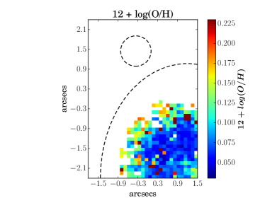
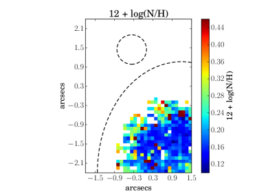
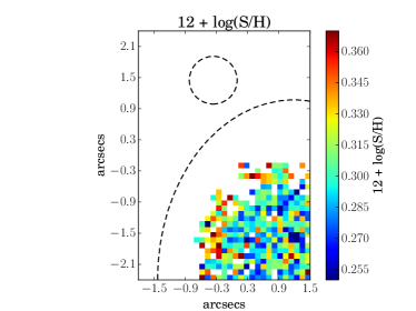
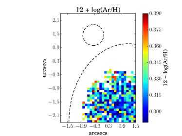
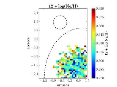
Figure 21: Uncertainty maps for the abundance maps presented in Figure 15.

Appendix B Flux and abundance tables corresponding to each annulus

Table 5 presents the observed and intrinsic flux values from integrated spectra of each annulus described in Section 3.5.3. The abundances and abundance ratios within each annulus are presented in Table 6.

Table 5: Emission line measurements (relative to H$\beta$ = 100) for the integrated spectrum of each annulus shown in Figure 14. Line fluxes (F_λ) are extinction corrected using E(B-V) to calculate F_λ.

Line	$\lambda_{air}$	$F(A)_{\lambda}$	$I(A)_{\lambda}$	$F(B)_{\lambda}$	$I(B)_{\lambda}$	$F(C)_{\lambda}$	$I(C)_{\lambda}$	$F(D)_{\lambda}$	$I(D)_{\lambda}$	$F(E)_{\lambda}$	$I(E)_{\lambda}$	$F(F)_{\lambda}$	$I(F)_{\lambda}$
[NIII]	3868.76	$27.11\pm 1.75$	$28.82\pm 2.04$	$26.63\pm 1.23$	$28.18\pm 1.52$	$24.13\pm 1.50$	$25.55\pm 1.72$	$26.22\pm 1.88$	$27.34\pm 2.09$	$23.62\pm 2.74$	$24.94\pm 3.01$	$19.29\pm 4.12$	$19.98\pm 4.32$
$H\gamma$	4340.47	$44.05\pm 0.56$	$45.42\pm 1.36$	$44.79\pm 0.55$	$46.07\pm 1.34$	$44.50\pm 0.58$	$45.78\pm 1.27$	$45.53\pm 0.76$	$46.48\pm 1.40$	$46.47\pm 0.85$	$47.75\pm 1.71$	$47.81\pm 1.04$	$48.65\pm 1.94$
$[OIII]$	4363.21	$9.38\pm 0.30$	$9.66\pm 0.40$	$9.46\pm 0.44$	$9.72\pm 0.52$	$9.21\pm 0.31$	$9.46\pm 0.40$	$8.53\pm 0.41$	$8.70\pm 0.48$	$8.58\pm 0.86$	$8.81\pm 0.93$	$6.71\pm 1.17$	$6.82\pm 1.22$
$H\beta$	4861.33	$100.00\pm 0.49$	$100.00\pm 1.86$	$100.00\pm 0.48$	$100.00\pm 1.81$	$100.00\pm 0.43$	$100.00\pm 1.67$	$100.00\pm 0.47$	$100.00\pm 1.72$	$100.00\pm 0.58$	$100.00\pm 2.11$	$100.00\pm 0.65$	$100.00\pm 2.31$
$[OIII]$	4958.92	$130.21\pm 0.95$	$129.57\pm 3.38$	$129.92\pm 0.90$	$129.32\pm 3.29$	$126.28\pm 0.83$	$125.70\pm 2.96$	$118.76\pm 0.74$	$118.36\pm 2.85$	$111.56\pm 0.87$	$111.07\pm 3.27$	$100.63\pm 0.83$	$100.34\pm 3.22$
$[OIII]$	5006.84	$388.09\pm 2.75$	$385.12\pm 9.97$	$385.75\pm 2.64$	$383.02\pm 9.68$	$374.54\pm 2.35$	$371.88\pm 8.68$	$353.61\pm 2.30$	$351.76\pm 8.43$	$330.75\pm 2.41$	$328.50\pm 9.57$	$300.52\pm 2.35$	$299.20\pm 9.50$
$HeI$	5875.67	$10.67\pm 0.17$	$10.18\pm 0.28$	$10.78\pm 0.15$	$10.32\pm 0.27$	$10.64\pm 0.18$	$10.19\pm 0.27$	$10.67\pm 0.20$	$10.33\pm 0.29$	$10.65\pm 0.23$	$10.21\pm 0.35$	$10.40\pm 0.30$	$10.12\pm 0.41$
$[OI]$	6300.3	$1.44\pm 0.07$	$1.36\pm 0.07$	$1.36\pm 0.05$	$1.28\pm 0.05$	$1.74\pm 0.06$	$1.64\pm 0.06$	$2.09\pm 0.08$	$2.00\pm 0.09$	$2.77\pm 0.10$	$2.62\pm 0.12$	$3.35\pm 0.16$	$3.23\pm 0.18$
$[SIII]$	6312.1	$1.54\pm 0.07$	$1.45\pm 0.08$	$1.47\pm 0.05$	$1.39\pm 0.06$	$1.43\pm 0.05$	$1.35\pm 0.06$	$1.51\pm 0.07$	$1.45\pm 0.07$	$1.51\pm 0.07$	$1.42\pm 0.08$	$1.25\pm 0.10$	$1.20\pm 0.11$
$[NII]$	6548.03	$0.81\pm 0.45$	$0.76\pm 0.42$	$0.90\pm 0.44$	$0.84\pm 0.42$	$1.04\pm 0.43$	$0.98\pm 0.40$	$1.07\pm 0.37$	$1.02\pm 0.36$	$1.20\pm 0.41$	$1.13\pm 0.39$	$1.58\pm 0.37$	$1.51\pm 0.36$
$H\alpha$	6562.8	$307.16\pm 1.73$	$286.00\pm 6.42$	$305.53\pm 1.68$	$286.00\pm 6.27$	$305.63\pm 1.55$	$286.00\pm 5.79$	$300.28\pm 1.56$	$286.00\pm 5.94$	$304.73\pm 1.94$	$286.00\pm 7.27$	$297.93\pm 2.07$	$286.00\pm 7.93$
$[NII]$	6583.41	$2.14\pm 0.45$	$1.99\pm 0.42$	$2.23\pm 0.44$	$2.08\pm 0.42$	$2.62\pm 0.43$	$2.45\pm 0.40$	$2.99\pm 0.37$	$2.85\pm 0.36$	$3.82\pm 0.41$	$3.59\pm 0.40$	$3.95\pm 0.37$	$3.79\pm 0.37$
$HeI$	6678.15	$2.92\pm 0.07$	$2.71\pm 0.08$	$2.87\pm 0.05$	$2.68\pm 0.07$	$2.88\pm 0.06$	$2.69\pm 0.08$	$2.87\pm 0.07$	$2.73\pm 0.09$	$2.85\pm 0.09$	$2.66\pm 0.10$	$2.76\pm 0.15$	$2.64\pm 0.16$
$[SII]$	6716.47	$6.05\pm 0.09$	$5.61\pm 0.15$	$6.13\pm 0.07$	$5.71\pm 0.14$	$7.21\pm 0.07$	$6.72\pm 0.15$	$8.82\pm 0.10$	$8.38\pm 0.19$	$11.04\pm 0.12$	$10.32\pm 0.28$	$12.79\pm 0.17$	$12.25\pm 0.36$
$[SII]$	6730.85	$4.42\pm 0.09$	$4.09\pm 0.12$	$4.57\pm 0.07$	$4.25\pm 0.11$	$5.15\pm 0.07$	$4.79\pm 0.11$	$6.11\pm 0.09$	$5.80\pm 0.15$	$7.79\pm 0.11$	$7.27\pm 0.21$	$9.12\pm 0.16$	$8.72\pm 0.28$
$[ArIII]$	7135.8	$4.11\pm 0.07$	$3.76\pm 0.10$	$4.11\pm 0.05$	$3.79\pm 0.09$	$4.09\pm 0.09$	$3.77\pm 0.11$	$4.16\pm 0.07$	$3.91\pm 0.10$	$4.32\pm 0.08$	$3.99\pm 0.12$	$4.13\pm 0.11$	$3.92\pm 0.15$
$[OII]$	7318.92	$1.31\pm 0.07$	$1.19\pm 0.07$	$1.31\pm 0.08$	$1.20\pm 0.07$	$1.49\pm 0.08$	$1.36\pm 0.08$	$1.66\pm 0.10$	$1.56\pm 0.09$	$2.01\pm 0.12$	$1.85\pm 0.12$	$2.18\pm 0.19$	$2.06\pm 0.18$
$[OII]$	7329.66	$1.11\pm 0.07$	$1.01\pm 0.06$	$1.10\pm 0.07$	$1.01\pm 0.07$	$1.17\pm 0.07$	$1.08\pm 0.07$	$1.31\pm 0.08$	$1.22\pm 0.08$	$1.63\pm 0.11$	$1.50\pm 0.11$	$1.74\pm 0.17$	$1.65\pm 0.16$
E(B-V)		$0.069\pm 0.005$		$0.063\pm 0.005$		$0.064\pm 0.005$		$0.047\pm 0.005$		$0.061\pm 0.006$		$0.039\pm 0.007$
F(H$\beta$)		$12.61\pm 0.06$	$15.83\pm 0.29$	$28.6\pm 0.14$	$35.25\pm 0.64$	$26.83\pm 0.12$	$33.14\pm 0.57$	$17.07\pm 0.08$	$19.94\pm 0.34$	$13.50\pm 0.08$	$16.53\pm 0.35$	$10.26\pm 0.07$	$11.68\pm 0.27$

Table 6: Summary of nebular diagnostics, ionic abundances, elemental abundances and abundance ratios obtained from the integrated spectra of annuli (A, B, C, D, E, F) shown in Figure 14.

Parameter	A	B	C	D	E	F
Te([OIII]) ($X$ 104 K)	$1.69\pm 0.04$	$1.70\pm 0.04$	$1.70\pm 0.04$	$1.67\pm 0.05$	$1.75\pm 0.11$	$1.60\pm 0.15$
Te([OII]) ($X$ 104 K)	$1.58\pm 0.02$	$1.57\pm 0.09$	$1.59\pm 0.03$	$1.58\pm 0.04$	$1.62\pm 0.07$	$1.53\pm 0.09$
Te([NII]) ($X$ 104 K)	$1.41\pm 0.01$	$1.41\pm 0.02$	$1.41\pm 0.01$	$1.40\pm 0.02$	$1.43\pm 0.04$	$1.38\pm 0.06$
Te([SIII]) ($X$ 104 K)	$1.69\pm 0.04$	$1.70\pm 0.05$	$1.70\pm 0.05$	$1.67\pm 0.06$	$1.76\pm 0.13$	$1.59\pm 0.19$
Ne([SII]) (cm-3)	$<$ 50	$60\pm 14$	$<$ 50	$<$ 50	$<$ 50	$<$ 50
12 + log(O+/H+)	$7.07\pm 0.03$	$7.10\pm 0.11$	$7.11\pm 0.04$	$7.18\pm 0.05$	$7.21\pm 0.08$	$7.36\pm 0.11$
12 + log(O2+/H+)	$7.51\pm 0.02$	$7.50\pm 0.03$	$7.49\pm 0.03$	$7.48\pm 0.03$	$7.40\pm 0.06$	$7.45\pm 0.10$
12 + log(O/H)	$7.64\pm 0.02$	$7.64\pm 0.04$	$7.64\pm 0.02$	$7.65\pm 0.03$	$7.62\pm 0.05$	$7.71\pm 0.07$
12 + log(N+/H+)	$5.28\pm 0.08$	$5.29\pm 0.04$	$5.36\pm 0.04$	$5.44\pm 0.04$	$5.52\pm 0.04$	$5.58\pm 0.04$
ICF (N+)	$3.73\pm 0.34$	$3.53\pm 0.94$	$3.39\pm 0.33$	$2.96\pm 0.36$	$2.56\pm 0.57$	$2.22\pm 0.67$
12 + log(N/H)	$5.85\pm 0.08$	$5.84\pm 0.12$	$5.89\pm 0.06$	$5.91\pm 0.07$	$5.93\pm 0.11$	$5.92\pm 0.14$
log(N/O)	$-1.79\pm 0.09$	$-1.80\pm 0.12$	$-1.74\pm 0.06$	$-1.75\pm 0.07$	$-1.69\pm 0.12$	$-1.78\pm 0.16$
S+/H+ ($X$ 107)	$0.93\pm 0.03$	$0.97\pm 0.10$	$1.10\pm 0.04$	$1.37\pm 0.06$	$1.62\pm 0.13$	$2.14\pm 0.23$
S2+/H+ ($X$ 107)	$5.33\pm 0.49$	$5.02\pm 0.51$	$4.84\pm 0.42$	$5.45\pm 0.62$	$4.66\pm 0.97$	$5.24\pm 1.89$
ICF (S+ + S2+)	$1.15\pm 0.01$	$1.13\pm 0.04$	$1.13\pm 0.02$	$1.10\pm 0.02$	$1.07\pm 0.02$	$1.05\pm 0.03$
12 + log(S/H)	$5.86\pm 0.03$	$5.83\pm 0.04$	$5.83\pm 0.03$	$5.87\pm 0.04$	$5.83\pm 0.07$	$5.89\pm 0.12$
log(S/O)	$-1.78\pm 0.04$	$-1.81\pm 0.06$	$-1.81\pm 0.04$	$-1.78\pm 0.05$	$-1.79\pm 0.09$	$-1.82\pm 0.13$
Ne2+/H+ ($X$ 105)	$0.57\pm 0.05$	$0.55\pm 0.05$	$0.50\pm 0.05$	$0.55\pm 0.06$	$0.45\pm 0.09$	$0.45\pm 0.15$
ICF (Ne2+)	$1.09\pm 0.00$	$1.09\pm 0.01$	$1.10\pm 0.00$	$1.10\pm 0.01$	$1.12\pm 0.02$	$1.14\pm 0.04$
12 + log(Ne/H)	$6.79\pm 0.04$	$6.78\pm 0.04$	$6.74\pm 0.04$	$6.78\pm 0.05$	$6.70\pm 0.09$	$6.71\pm 0.16$
log(Ne/O)	$-0.85\pm 0.04$	$-0.86\pm 0.05$	$-0.90\pm 0.05$	$-0.87\pm 0.06$	$-0.92\pm 0.10$	$-1.00\pm 0.17$
Ar2+/H+ ($X$ 107)	$1.24\pm 0.06$	$1.23\pm 0.07$	$1.23\pm 0.06$	$1.31\pm 0.08$	$1.23\pm 0.14$	$1.43\pm 0.30$
ICF (Ar2+)	$1.14\pm 0.00$	$1.14\pm 0.01$	$1.14\pm 0.00$	$1.15\pm 0.01$	$1.17\pm 0.03$	$1.20\pm 0.05$
12 + log(Ar/H)	$5.15\pm 0.02$	$5.15\pm 0.03$	$5.15\pm 0.02$	$5.18\pm 0.03$	$5.16\pm 0.05$	$5.23\pm 0.09$
log(Ar/O)	$-2.49\pm 0.03$	$-2.49\pm 0.05$	$-2.49\pm 0.03$	$-2.47\pm 0.04$	$-2.46\pm 0.07$	$-2.48\pm 0.12$

References

- Aggarwal & Keenan (1999) Aggarwal K. M., Keenan F. P., 1999, ApJS, 123, 311
- Allington-Smith et al. (2002) Allington-Smith J., et al., 2002, PASP, 114, 892
- Aloisi et al. (2005) Aloisi A., van der Marel R. P., Mack J., Leitherer C., Sirianni M., Tosi M., 2005, ApJ, 631, L45
- Astropy Collaboration et al. (2013) Astropy Collaboration et al., 2013, A&A, 558, A33
- Baldwin et al. (1981) Baldwin J. A., Phillips M. M., Terlevich R., 1981, PASP, 93, 5
- Belfiore et al. (2017) Belfiore F., et al., 2017, MNRAS, 469, 151
- Berg et al. (2013) Berg D. A., Skillman E. D., Garnett D. R., Croxall K. V., Marble A. R., Smith J. D., Gordon K., Kennicutt Jr. R. C., 2013, ApJ, 775, 128
- Berg et al. (2015) Berg D. A., Skillman E. D., Croxall K. V., Pogge R. W., Moustakas J., Johnson-Groh M., 2015, ApJ, 806, 16
- Cantin et al. (2010) Cantin S., Robert C., Mollá M., Pellerin A., 2010, MNRAS, 404, 811
- Dors et al. (2016) Dors O. L., Pérez-Montero E., Hägele G. F., Cardaci M. V., Krabbe A. C., 2016, MNRAS, 456, 4407
- Fitzpatrick (1999) Fitzpatrick E. L., 1999, PASP, 111, 63
- García-Benito et al. (2010) García-Benito R., et al., 2010, MNRAS, 408, 2234
- Garnett (1992) Garnett D. R., 1992, AJ, 103, 1330
- Guseva et al. (2003) Guseva N. G., Papaderos P., Izotov Y. I., Green R. F., Fricke K. J., Thuan T. X., Noeske K. G., 2003, A&A, 407, 105
- Hägele et al. (2006) Hägele G. F., Pérez-Montero E., Díaz Á. I., Terlevich E., Terlevich R., 2006, MNRAS, 372, 293
- Hägele et al. (2008) Hägele G. F., Díaz Á. I., Terlevich E., Terlevich R., Pérez-Montero E., Cardaci M. V., 2008, MNRAS, 383, 209
- Henry & Worthey (1999) Henry R. B. C., Worthey G., 1999, PASP, 111, 919
- Ho et al. (2015) Ho I.-T., Kudritzki R.-P., Kewley L. J., Zahid H. J., Dopita M. A., Bresolin F., Rupke D. S. N., 2015, MNRAS, 448, 2030
- Hong et al. (2013) Hong S., Calzetti D., Gallagher III J. S., Martin C. L., Conselice C. J., Pellerin A., 2013, ApJ, 777, 63
- Hook et al. (2004) Hook I. M., Jørgensen I., Allington-Smith J. R., Davies R. L., Metcalfe N., Murowinski R. G., Crampton D., 2004, PASP, 116, 425
- Izotov & Thuan (1999) Izotov Y. I., Thuan T. X., 1999, ApJ, 511, 639
- Izotov et al. (1994) Izotov Y. I., Thuan T. X., Lipovetsky V. A., 1994, ApJ, 435, 647
- Izotov et al. (2006) Izotov Y. I., Stasińska G., Meynet G., Guseva N. G., Thuan T. X., 2006, A&A, 448, 955
- James et al. (2009) James B. L., Tsamis Y. G., Barlow M. J., Westmoquette M. S., Walsh J. R., Cuisinier F., Exter K. M., 2009, MNRAS, 398, 2
- James et al. (2010) James B. L., Tsamis Y. G., Barlow M. J., 2010, MNRAS, 401, 759
- James et al. (2013a) James B. L., Tsamis Y. G., Barlow M. J., Walsh J. R., Westmoquette M. S., 2013a, MNRAS, 428, 86
- James et al. (2013b) James B. L., Tsamis Y. G., Walsh J. R., Barlow M. J., Westmoquette M. S., 2013b, MNRAS, 430, 2097
- James et al. (2015) James B. L., Koposov S., Stark D. P., Belokurov V., Pettini M., Olszewski E. W., 2015, MNRAS, 448, 2687
- Kauffmann et al. (2003) Kauffmann G., et al., 2003, MNRAS, 346, 1055
- Kehrig et al. (2013) Kehrig C., et al., 2013, MNRAS, 432, 2731
- Kennicutt (1998) Kennicutt Jr. R. C., 1998, ApJ, 498, 541
- Kewley et al. (2001) Kewley L. J., Dopita M. A., Sutherland R. S., Heisler C. A., Trevena J., 2001, ApJ, 556, 121
- Kewley et al. (2010) Kewley L. J., Rupke D., Zahid H. J., Geller M. J., Barton E. J., 2010, ApJ, 721, L48
- Kniazev et al. (2003) Kniazev A. Y., Grebel E. K., Hao L., Strauss M. A., Brinkmann J., Fukugita M., 2003, ApJ, 593, L73
- Kumari et al. (2017) Kumari N., James B. L., Irwin M. J., 2017, MNRAS, 470, 4618
- Kumari et al. (2018) Kumari N., James B. L., Irwin M. J., Amorín R., Pérez-Montero E., 2018, preprint, (arXiv:1802.04797)
- Lagos et al. (2012) Lagos P., Telles E., Nigoche Netro A., Carrasco E. R., 2012, MNRAS, 427, 740
- Lagos et al. (2014) Lagos P., Papaderos P., Gomes J. M., Smith Castelli A. V., Vega L. R., 2014, A&A, 569, A110
- Lagos et al. (2016) Lagos P., Demarco R., Papaderos P., Telles E., Nigoche-Netro A., Humphrey A., Roche N., Gomes J. M., 2016, MNRAS, 456, 1549
- Lelli et al. (2014) Lelli F., Verheijen M., Fraternali F., 2014, A&A, 566, A71
- Lind et al. (2011) Lind K., Charbonnel C., Decressin T., Primas F., Grundahl F., Asplund M., 2011, A&A, 527, A148
- López-Hernández et al. (2013) López-Hernández J., Terlevich E., Terlevich R., Rosa-González D., Díaz Á., García-Benito R., Vílchez J., Hägele G., 2013, MNRAS, 430, 472
- López-Sánchez & Esteban (2010) López-Sánchez Á. R., Esteban C., 2010, A&A, 517, A85
- López-Sánchez et al. (2007) López-Sánchez Á. R., Esteban C., García-Rojas J., Peimbert M., Rodríguez M., 2007, ApJ, 656, 168
- Ly et al. (2016) Ly C., Malhotra S., Malkan M. A., Rigby J. R., Kashikawa N., de los Reyes M. A., Rhoads J. E., 2016, ApJS, 226, 5
- Monreal-Ibero et al. (2011) Monreal-Ibero A., Relaño M., Kehrig C., Pérez-Montero E., Vílchez J. M., Kelz A., Roth M. M., Streicher O., 2011, MNRAS, 413, 2242
- Pérez-Montero (2017) Pérez-Montero E., 2017, PASP, 129, 043001
- Pérez-Montero & Contini (2009) Pérez-Montero E., Contini T., 2009, MNRAS, 398, 949
- Pérez-Montero & Díaz (2007) Pérez-Montero E., Díaz Á. I., 2007, MNRAS, 377, 1195
- Pérez-Montero et al. (2007) Pérez-Montero E., Hägele G. F., Contini T., Díaz Á. I., 2007, MNRAS, 381, 125
- Pérez-Montero et al. (2011) Pérez-Montero E., et al., 2011, A&A, 532, A141
- Pilkington et al. (2012) Pilkington K., et al., 2012, A&A, 540, A56
- Sánchez et al. (2012) Sánchez S. F., et al., 2012, A&A, 546, A2
- Schlafly & Finkbeiner (2011) Schlafly E. F., Finkbeiner D. P., 2011, ApJ, 737, 103
- Stasińska (1978) Stasińska G., 1978, A&A, 66, 257
- Sternberg et al. (2003) Sternberg A., Hoffmann T. L., Pauldrach A. W. A., 2003, ApJ, 599, 1333
- Thuan et al. (1999) Thuan T. X., Izotov Y. I., Foltz C. B., 1999, ApJ, 525, 105
- Vílchez & Iglesias-Páramo (1998) Vílchez J. M., Iglesias-Páramo J., 1998, ApJ, 508, 248
- Westmoquette et al. (2013) Westmoquette M. S., James B., Monreal-Ibero A., Walsh J. R., 2013, A&A, 550, A88
- Woosley & Weaver (1995) Woosley S. E., Weaver T. A., 1995, ApJS, 101, 181