Weak Lensing Effect on CMB in the Presence of a Dipole Anisotropy

Abstract

We investigate weak lensing effect on cosmic microwave background (CMB) in the presence of dipole anisotropy. The approach of flat-sky approximation is considered. We determine the functions $\sigma_{0}^{2}$ and $\sigma_{2}^{2}$ that appear in expressions of the lensed CMB power spectrum in the presence of a dipole anisotropy. We determine the correction to B-mode power spectrum which is found to be appreciable at low multipoles ($l$). However, the temperature and E-mode power spectrum are not altered significantly.

I Introduction

In unveiling the dynamics and contents of the universe, cosmic microwave background radiation has been one of the essential tools. CMB constrains cosmological parameters, and it provides a path in developing modern cosmology. The precision level of the experiments for the CMB spectrum and hence the accuracy of prediction of a theoretical model have been increasing year by year. The CMB anisotropy can be determined by the Physics of last scattering surface (LSS) and the medium effects due to the propagation of photons from LSS to the observer. The primary contribution to the anisotropy is due to the strength of the metric perturbations at LSS. Some other effects such as ISW effect, reionization, quadrupole distributions give additional modifications. Lensing is an effect which is associated with the geodesics of photons from LSS to us. It can be considered as a secondary contribution in modifying CMB anisotropy, and it must be taken into account to reliably predict the CMB signal. The lensing gives a very small contribution on the reionization and the ISW signal as these are associated with the large scale. However, on degree-scale of primary acoustic peaks, weak lensing effect is expected at the order of arc minute on the CMB spectrum Lewis:2006fu .

In this paper, we are interested in the weak lensing effect on the CMB spectrum arising due to a dipole distribution in the Newtonian potential. The unexpected observation of anisotropy at large scale leads us to study the implications of such model. In WMAP data, some of the anomalies were discovered Bennett:2012zja . These anomalies include the alignment between low multipoles Tegmark:2003ve ; Copi:2003kt ; Land:2005ad , large cold spot in the southern hemisphere Vielva:2003et ; Mukherjee:2004in ; Cruz:2004ce , hemisphere power asymmetry Eriksen:2003db . The Planck data has further confirmed the existence of such anomalies Ade:2013nlj . According to Planck data, the dipole modulation of power lies in the range $l=2-600$ at $1.1-3.5\sigma$. In addition, it confirmed octopole-quadrupole alignment at $98\%$ level and a power deficit below $l=40$. Other observables, such as, radio polarization from radio galaxies and optical polarization of quasars also indicate anisotropy at the large scale. Remarkably, orientations of dipole axis of radio polarization Jain:1998kf , dipole, quadrupole and octopole axes of the CMB Ralston:2003pf and the direction of alignment of the pattern of two-point correlation in the optical polarization Jain:2003sg all point towards the Virgo direction. The model with dipole anisotropy we study in this paper is proposed by Gordon Gordon:2005ai . It has also been studied in Refs. Erickcek:2008sm ; Liddle:2013czu ; Ghosh:2013blq . Furthermore, the CMB spectrum have been investigated in Refs. Kothari:2015tqa ; Ghosh:2015qta ; Ghosh:2018apx in this model. In this paper, we study weak lensing effect on the CMB spectrum with the flat-sky approximation Zaldarriaga:1998ar . In Sec. (II), we generalize the two-point correction function due to the weak lensing with the dipole anisotropy. In this section, we also calculate the expectation value of a term which arises due to the isotropic part of lensing potential. In Sec. (III), we estimate the modification to this term in presence of the dipole anisotropy. In Sec. (IV), we obtain expressions for CMB power spectrum. In Sec. (V), we conclude.

II Gravitational Lensing Effect on Two-Point Correlation Functions in the Presence of Dipole Anisotropy

The observed CMB spectrum is different from that produced at LSS due to the lensing effect. These are related as Zaldarriaga:1998ar

$$X(\hbox{\boldmath{$\theta$}}) = \tilde{X}(\hbox{\boldmath{$\theta$}}+\delta\hbox{\boldmath{$\theta$}})$$ (1)

$$= \frac{1}{(2\pi)^{2}}\int d^{2}{\hbox{\boldmath{$l$}}}e^{i{\hbox{\boldmath{$l$}}}.(\hbox{\boldmath{$\theta$}}+\delta\hbox{\boldmath{$\theta$}})}\tilde{X}({\hbox{\boldmath{$l$}}}),$$

where, $X(\hbox{\boldmath{$\theta$}})$ is the observed physical quantity such as the temperature $T(\hbox{\boldmath{$\theta$}})$, the stokes parameters $Q(\hbox{\boldmath{$\theta$}})$ and $U(\hbox{\boldmath{$\theta$}})$ etc., whereas $\tilde{X}(\hbox{\boldmath{$\theta$}}+\delta\hbox{\boldmath{$\theta$}})$ is the corresponding physical quantity produced at LSS. Writing these variables in the explicit form, we have,

$$T({\hbox{\boldmath{$\theta$}}}) = \tilde{T}(\hbox{\boldmath{$\theta$}}+\delta\hbox{\boldmath{$\theta$}})$$ (2)

$$= \frac{1}{(2\pi)^{2}}\int d^{2}{\hbox{\boldmath{$l$}}}\ e^{i{\hbox{\boldmath{$l$}}}\cdot({\hbox{\boldmath{$\theta$}}}+\delta{\hbox{\boldmath{$\theta$}}})}\tilde{T}({\hbox{\boldmath{$l$}}}),$$

$$Q({\hbox{\boldmath{$\theta$}}}) = \tilde{Q}(\hbox{\boldmath{$\theta$}}+\delta\hbox{\boldmath{$\theta$}})$$ (3)

$$= \frac{1}{(2\pi)^{2}}\int d^{2}{\hbox{\boldmath{$l$}}}\ e^{i{\hbox{\boldmath{$l$}}}\cdot({\hbox{\boldmath{$\theta$}}}+\delta{\hbox{\boldmath{$\theta$}}})}\tilde{Q}({\hbox{\boldmath{$l$}}}),$$

$$= \frac{1}{(2\pi)^{2}}\int d^{2}{\hbox{\boldmath{$l$}}}\ e^{i{l}\cdot({\hbox{\boldmath{$\theta$}}}+\delta{\hbox{\boldmath{$\theta$}}})}\Big{[}\tilde{E}({\hbox{\boldmath{$l$}}})\cos(2\phi_{\hbox{\boldmath{$l$}}})-\tilde{B}({\hbox{\boldmath{$l$}}})\sin(2\phi_{\hbox{\boldmath{$l$}}})\Big{]},$$

$$U({\hbox{\boldmath{$\theta$}}}) = \tilde{U}(\hbox{\boldmath{$\theta$}}+\delta\hbox{\boldmath{$\theta$}})$$ (4)

$$= \frac{1}{(2\pi)^{2}}\int d^{2}{\hbox{\boldmath{$l$}}}\ e^{i{\hbox{\boldmath{$l$}}}\cdot({\hbox{\boldmath{$\theta$}}}+\delta{\hbox{\boldmath{$\theta$}}})}\tilde{U}({\hbox{\boldmath{$l$}}})$$

$$= \frac{1}{(2\pi)^{2}}\int d^{2}{\hbox{\boldmath{$l$}}}\ e^{i{\hbox{\boldmath{$l$}}}\cdot({\hbox{\boldmath{$\theta$}}}+\delta{\hbox{\boldmath{$\theta$}}})}\Big{[}\tilde{E}({\hbox{\boldmath{$l$}}})\sin(2\phi_{\hbox{\boldmath{$l$}}})+\tilde{B}({\hbox{\boldmath{$l$}}})\cos(2\phi_{\hbox{\boldmath{$l$}}})\Big{]},$$

where, the standard definitions of $Q({\hbox{\boldmath{$l$}}})$ and $U({\hbox{\boldmath{$l$}}})$ are used. Using above Eqs. (2), (3) and (4), we can compute correlation function of such quantities at two points $\theta_{1}$ and $\theta_{2}$. In general, these two points can be anywhere on the two dimensional plane in small scale limit formalism. However for simplicity, we rotate our frame such that these two points fall on $x-$axis. We can also shift $\theta_{1}$ at $\theta_{1}=0$ or $\theta_{2}$ at $\theta_{2}=0$ keeping other point at the separation of $\theta$. Now, the correlation function corresponding to the temperature is given by,

$$C_{T}(\theta) = <T({\hbox{\boldmath{$\theta$}}_{1}})T({\hbox{\boldmath{$\theta$}}_{2})}>$$ (5)

$$= <\tilde{T}({\hbox{\boldmath{$\theta$}}_{1}}+\delta{\hbox{\boldmath{$\theta$}}_{1}})\tilde{T}({\hbox{\boldmath{$\theta$}}_{2}}+\delta{\hbox{\boldmath{$\theta$}}_{2}})>$$

$$= \int\frac{d^{2}{\hbox{\boldmath{$l$}}}}{(2\pi)^{2}}e^{i{l}\theta\cos(\phi_{l})}<e^{i{\hbox{\boldmath{$l$}}}\cdot(\delta{\hbox{\boldmath{$\theta$}}_{1}}-\delta{\hbox{\boldmath{$\theta$}}_{2}})}>C_{\tilde{T}l},$$

where, we have used

$$<\tilde{Y}({\hbox{\boldmath{$l$}}})\tilde{Y}({\hbox{\boldmath{$l$}}}^{\prime})>=(2\pi)^{2}\tilde{C}_{Y{\hbox{\boldmath{$l$}}}}\delta^{2}({\hbox{\boldmath{$l$}}}-{\hbox{\boldmath{$l$}}}^{\prime}).$$ (6)

The vector quantity $l$ which is conjugate to $\theta$ makes the angle $\phi_{\hbox{\boldmath{$l$}}}$ with the $x-$axis. In the similar way, we obtain the following relation for $C_{Q}(\theta)$ and $C_{U}(\theta)$,

$$C_{Q}({\theta}) = \int{d^{2}{\hbox{\boldmath{$l$}}}\over(2\pi)^{2}}\ e^{il\theta\cos\phi_{l}}\langle e^{i{\hbox{\boldmath{$l$}}}\cdot(\delta{\hbox{\boldmath{$\theta$}}_{1}}-\delta{\hbox{\boldmath{$\theta$}}}_{2})}\ \rangle\ \ [C_{\tilde{E}l}\cos^{2}(2\phi_{\hbox{\boldmath{$l$}}})+C_{\tilde{B}l}\sin^{2}(2\phi_{\hbox{\boldmath{$l$}}})]$$

$$C_{U}({\theta}) = \int{d^{2}{\hbox{\boldmath{$l$}}}\over(2\pi)^{2}}\ e^{il\theta\cos\phi_{l}}\langle e^{i{\hbox{\boldmath{$l$}}}\cdot(\delta{\hbox{\boldmath{$\theta$}}_{1}}-\delta{\hbox{\boldmath{$\theta$}}}_{2})}\ \rangle\ \ [C_{\tilde{E}l}\sin^{2}(2\phi_{\hbox{\boldmath{$l$}}})+C_{\tilde{B}l}\cos^{2}(2\phi_{\hbox{\boldmath{$l$}}})].$$ (7)

The quantity $\langle e^{i{\hbox{\boldmath{$l$}}}\cdot(\delta{\hbox{\boldmath{$\theta$}}_{1}}-\delta{\hbox{\boldmath{$\theta$}}}_{2})}\ \rangle$ is important since the weak lensing effect with the dipole anisotropy is involved here. We compute this quantity following Ref. Zaldarriaga:1998ar by adding the dipole matter distribution. Let us define the deflection angles as $\alpha=\delta\theta_{1}$ and $\alpha^{\prime}=\delta\theta_{2}$. The deflection angle is given by,

$$\alpha=\nabla_{\hat{n}}\psi(\hat{n}),$$ (8)

where, $\nabla_{\hat{n}}$ is angular derivative, $\hat{n}$ is direction of observation and $\psi(\hat{n})$ is lensing potential and it is connected to gravitational potential ${\hbox{\boldmath{$\psi$}}}(\chi\hat{n},\eta_{0}-\chi)$ via,

$$\psi(\hat{\eta})\equiv-2\int^{\chi^{*}}_{0}d\chi\frac{f_{K}(\chi^{*}-\chi)}{f_{K}(\chi^{*})f_{K}(\chi)}{\hbox{\boldmath{$\psi$}}}(\chi\hat{n},\eta_{0}-\chi),$$ (9)

where, $\chi^{*}$ is conformal distance of LSS from us. In our case, the gravitational potential has two parts, the homogeneous part ${\hbox{\boldmath{$\psi$}}}^{h}$and part ${\hbox{\boldmath{$\psi$}}}^{d}$ corresponding to dipole distribution:

$${\hbox{\boldmath{$\psi$}}}={\hbox{\boldmath{$\psi$}}}^{h}+{\hbox{\boldmath{$\psi$}}}^{d}.$$ (10)

Expanding ${\hbox{\boldmath{$\psi$}}}^{h}$ by Fourier expansion, we have

$${\hbox{\boldmath{$\psi$}}}(\theta)=\frac{1}{(2\pi)^{2}}\int d^{2}{\hbox{\boldmath{$l$}}}e^{i{\hbox{\boldmath{$l$}}}\cdot\hbox{\boldmath{$\theta$}}}{\hbox{\boldmath{$\psi$}}}^{h}_{\hbox{\boldmath{$l$}}}+{\hbox{\boldmath{$\psi$}}}^{d}.$$ (11)

Now we calculate the correlation tensor,

$$\langle\alpha_{i}\alpha^{\prime}_{j}\rangle=\langle\nabla_{i}\psi\nabla_{j}\psi^{\prime}\rangle.$$ (12)

Using above Eq. (12), we obtain

$$\langle\alpha_{i}\alpha^{\prime}_{j}\rangle = \langle\nabla_{i}{\psi}\nabla_{j}{\psi}^{\prime}\rangle,$$ (13)

$$= \langle\nabla_{i}{\psi^{h}}\nabla_{j}{\psi^{\prime}{{}^{h}}}\rangle+\langle\nabla_{i}{\psi^{d}}\nabla_{j}{\psi^{\prime d}}\rangle,$$

$$= \int\frac{d^{2}{\hbox{\boldmath{$l$}}}}{(2\pi)^{2}}{\hbox{\boldmath{$l$}}}_{i}{\hbox{\boldmath{$l$}}}_{j}e^{i{\hbox{\boldmath{$l$}}}\cdot{\hbox{\boldmath{$\theta$}}}}C_{l}^{\psi\psi^{\prime}}+\langle\nabla_{i}{\psi^{d}}\nabla_{j}{\psi^{\prime d}}\rangle,$$

where, $\langle{\psi}^{h}_{\hbox{\boldmath{$l$}}}{\psi}^{h*}_{\hbox{\boldmath{$l$}}^{\prime}}\rangle=(2\pi)^{2}\delta^{2}({\hbox{\boldmath{$l$}}}-{\hbox{\boldmath{$l$}}^{\prime}})C_{l}^{\psi\psi^{\prime}}$ is used. In Eq. (13), we denote the first term which is the homogeneous part by $\langle\alpha^{h}_{i}\alpha^{\prime h}_{j}\rangle$. The correlation function $\langle\alpha^{h}_{i}\alpha^{\prime h}_{j}\rangle$ should be proportional to $\delta_{ij}$ and the trace-free tensor given by $\hat{r}_{<i}\hat{r}_{j>}=\hat{r}_{i}\hat{r}_{j}-\frac{1}{2}\delta_{ij}$. Using this fact, the first homogeneous part simplifies as

$$\int\frac{d^{2}{\hbox{\boldmath{$l$}}}}{(2\pi)^{2}}{\hbox{\boldmath{$l$}}}_{i}{\hbox{\boldmath{$l$}}}_{j}e^{i{\hbox{\boldmath{$l$}}}\cdot{\hbox{\boldmath{$\theta$}}}}C_{l}^{\psi\psi^{\prime}}=\frac{1}{2}C_{gl}\delta_{ij}-C_{gl,2}\hat{r}_{<i}\hat{r}_{j>},$$ (14)

where,

$$C_{gl}(\theta)=\int{\frac{dl}{2\pi}l^{3}}C_{l}^{\psi\psi^{\prime}}J_{0}(l\theta),$$ (15)

$$C_{gl,2}(\theta)=\int{\frac{dl}{2\pi}l^{3}}C_{l}^{\psi\psi^{\prime}}J_{2}(l\theta).$$ (16)

Now we come to the term $\langle e^{i{\hbox{\boldmath{$l$}}}\cdot(\alpha-\alpha^{\prime})}\rangle$ in which we are interested in order to understand the lensing effects including dipole matter distribution. It can be shown that Lewis:2006fu

$$\langle e^{i{\hbox{\boldmath{$l$}}}\cdot(\alpha-\alpha^{\prime})}\rangle=e^{-\frac{1}{2}\langle[l\cdot(\alpha-\alpha^{\prime})]^{2}\rangle}.$$ (17)

Expanding the term $\langle[l\cdot(\alpha-\alpha^{\prime})]^{2}\rangle$, we have

$$\langle[l\cdot(\alpha-\alpha^{\prime})]^{2}\rangle = l^{i}l^{j}\langle(\alpha-\alpha^{\prime})_{i}(\alpha-\alpha^{\prime})_{j}\rangle$$ (18)

$$= l^{i}l^{j}\Big{[}\langle\alpha_{i}\alpha_{j}\rangle+\langle\alpha_{i}^{\prime}\alpha_{j}^{\prime}\rangle-2\langle\alpha_{i}\alpha_{j}^{\prime}\rangle\Big{]}$$

$$= l^{i}l^{j}\Big{[}\langle\alpha_{i}\alpha_{j}\rangle+\langle\alpha_{i}^{\prime}\alpha_{j}^{\prime}\rangle-2\langle\alpha_{i}\alpha_{j}^{\prime}\rangle\Big{]}^{h}+l^{i}l^{j}\Big{[}\langle\alpha_{i}\alpha_{j}\rangle+\langle\alpha_{i}^{\prime}\alpha_{j}^{\prime}\rangle-2\langle\alpha_{i}\alpha_{j}^{\prime}\rangle\Big{]}^{d}.$$

We obtain the terms due to homogeneous part as well as dipole part, since $\langle\alpha_{i}\alpha_{j}\rangle$, $\langle\alpha_{i}^{\prime}\alpha_{j}^{\prime}\rangle$ and $\langle\alpha_{i}\alpha_{j}^{\prime}\rangle$ all have two parts as in Eq. (13). Homogeneous part becomes

$$\langle[l\cdot(\alpha-\alpha^{\prime})]^{2}\rangle^{h} = l^{2}\Big{[}C_{gl}(0)-C_{gl}(\theta)+\cos(2\phi_{l})C_{gl,2}(\theta)\Big{]},$$ (19)

$$= l^{2}\Big{[}\sigma_{0}^{2}(\theta)+\sigma_{2}^{2}(\theta)\cos(2\phi_{l})\Big{]},$$

where, we define $\sigma_{0}^{2}(\theta)=C_{gl}(0)-C_{gl}(\theta)$ and $\sigma_{2}^{2}(\theta)=C_{gl,2}$. These notations, $\sigma_{0}^{2}(\theta)$ and $\sigma_{2}^{2}(\theta)$, have been used in the literature Zaldarriaga:1998ar .

III Dipole Anisotropy Correction

In this section, we estimate first the correction to $\langle[l\cdot(\alpha-\alpha^{\prime})]^{2}\rangle$ due to the dipole distribution. In Eq. (13), the additional second term is due to the dipole. To calculate it, we expand $\psi^{d}$ in $3$-dimensional Fourier space as follows Yu:2009bz ,

$$\psi^{d}(\eta^{*},\hat{n})=-2\int^{\chi^{*}}_{0}d\chi_{1}\frac{f_{K}(\chi^{*}-\chi_{1})}{f_{K}(\chi^{*})f_{K}(\chi_{1})}\int\frac{d^{3}k}{(2\pi)^{3}}{\hbox{\boldmath{$\psi$}}}^{d}({\hbox{\boldmath{$k$}}})e^{ik.(\eta_{0}-\eta_{1})\hat{n}}T_{\psi}(\eta_{1},k).$$ (20)

The dipole distribution is defined by the coefficient ${\hbox{\boldmath{$\psi$}}}^{d}_{\hbox{\boldmath{$k$}}}$ which is given by Ghosh:2013blq ,

$${\hbox{\boldmath{$\psi$}}}^{d}_{\hbox{\boldmath{$k$}}}=\frac{\beta}{2i}(2\pi)^{3}\Big{[}\delta^{3}({\hbox{\boldmath{$k$}}}-\kappa_{s}\hat{x})-\delta^{3}({\hbox{\boldmath{$k$}}}+\kappa_{s}\hat{x})\Big{]},$$ (21)

where, $\beta$ and $\kappa_{s}$ are two parameters which define the dipole. We consider the alignment of dipole in $x-$direction and we keep $\psi^{d}$ in generalized form of 3D. Now, we redefine the momentum $k$ in terms of $l$, by $\vec{l}=\chi^{*}\vec{k}$, $\int d^{3}k{\hbox{\boldmath{$\psi$}}}^{d}(k)\rightarrow\int d^{3}l{\hbox{\boldmath{$\psi$}}}^{d}(l)$ and $\frac{\eta_{0}-\eta}{\chi^{*}}=\frac{\chi}{\chi^{*}}=\omega$. In this definition,

$$\frac{{\hbox{\boldmath{$\psi$}}}^{d}(k)}{\chi^{*3}} = \frac{\beta}{2i}\frac{(2\pi)^{3}}{\chi^{*3}}\Big{[}\delta^{3}({\hbox{\boldmath{$k$}}}-\kappa_{s}\hat{x})-\delta^{3}({\hbox{\boldmath{$k$}}}+\kappa_{s}\hat{x})\Big{]}$$ (22)

$$= \frac{\beta}{2i}(2\pi)^{3}\Big{[}\delta^{3}(\chi^{*}{\hbox{\boldmath{$k$}}}-\chi^{*}\kappa_{s}\hat{x})-\delta^{3}(\chi^{*}{\hbox{\boldmath{$k$}}}+\chi^{*}\kappa_{s}\hat{x})\Big{]},$$

$$= \frac{\beta}{2i}(2\pi)^{3}\Big{[}\delta^{3}({\hbox{\boldmath{$l$}}}-\kappa\hat{x})-\delta^{3}({\hbox{\boldmath{$l$}}}+\kappa\hat{x})\Big{]}=\psi^{d}(l),$$

where, $\kappa=\chi*\kappa_{s}$. Under such definition, Eq. (20) can be written as,

$$\psi^{d}(\eta^{*},\hat{n})=-2\int^{\chi*}_{0}d\chi_{1}\frac{f_{K}(\chi^{*}-\chi_{1})}{f_{K}(\chi*)f_{K}(\chi_{1})}\int\frac{d^{3}l}{(2\pi)^{3}}\psi^{d}(l)e^{i{\hbox{\boldmath{$l$}}}.\hat{n}\omega}T_{\psi}(\eta_{1},l).$$ (23)

We assume that the transfer function is nearly unity for the large scale and set it as unity in the further calculation. We can now simplify the term $\langle\nabla_{i}{\psi^{d}}\nabla_{j}{\psi^{\prime d}}\rangle$ as follows,

$$<\nabla_{i}\psi^{d}(\eta^{*},\hat{n_{1}})\nabla_{j}\psi^{*d}(\eta^{*},\hat{n_{2}})>=4\int^{\chi^{*}}_{0}\int^{\chi^{*}}_{0}d\chi_{1}d\chi_{2}\frac{(\chi^{*}-\chi_{1})}{(\chi^{*}\chi_{1})}\frac{(\chi^{*}-\chi_{2})}{(\chi^{*}\chi_{2})}\times$$

$$\int\int d^{3}ld^{3}l^{\prime}\omega_{1}\omega_{2}l_{i}l_{j}^{\prime}\left(\frac{\beta^{2}}{4}\right)\Big{[}\delta^{3}(\vec{l}-\kappa\hat{x})\delta^{3}(\vec{l}-\kappa\hat{x})-\delta^{3}(\vec{l}-\kappa\hat{x})\delta^{3}(\vec{l}+\kappa\hat{x})$$

$$-\delta^{3}(\vec{l}+\kappa\hat{x})\delta^{3}(\vec{l}-\kappa\hat{x})+\delta^{3}(\vec{l}+\kappa\hat{x})\delta^{3}(\vec{l}+\kappa\hat{x})\Big{]}\times$$

$$e^{i\hat{l}.\hat{n_{1}}\omega_{1}}e^{-i\hat{l^{\prime}}.\hat{n_{2}}\omega_{2}}.$$ (24)

Here, $\eta$ is the conformal time at the point of observation. $\nabla_{i}$ has two components corresponding to the directions $x$ and $y$ and in the flat sky approximation equivalent to $\frac{\partial}{\ \partial{n_{x}}}$ and $\frac{\partial}{\ \partial{n_{y}}}$ respectively. Here $n_{x}$ and $n_{y}$ are x and y components of $\hat{n}$, the unit vector in the direction of observation from us. The two points of observation could be anywhere on the sphere, however, we consider these points on the great circle parallel to $x$-axis. The unit direction $\hat{n}$, which is given by

$$\hat{n}=\sin{\theta}\cos{\phi}\hat{x}+\sin{\theta}\sin{\phi}\hat{y}+\cos{\theta}\hat{z}$$ (25)

becomes $\sin{\theta}\hat{x}+\cos{\theta}\hat{z}$ ($\phi=0$) in this case. The momentum integrals contains four terms, we calculate these one by one. The first term is given by,

$$\frac{\beta^{2}}{4}\int\int d^{3}ld^{3}l^{\prime}\omega_{1}\omega_{2}l_{i}l_{j}^{\prime}\Big{[}\delta^{3}(\vec{l}-\kappa\hat{x})\delta^{3}(\vec{l^{\prime}}-\kappa\hat{x})\Big{]}e^{i\hat{l}.\hat{n_{1}}\omega_{1}}e^{-i\hat{l^{\prime}}.\hat{n_{2}}\omega_{2}}$$

$$=\frac{\beta^{2}}{4}\omega_{1}\omega_{2}\kappa^{2}\delta_{i}^{x}\delta_{j}^{x}e^{i\kappa(\omega_{1}\sin\theta_{1}-\omega_{2}\sin\theta_{2})},$$ (26)

similarly second, third and last terms can be written as,

$$-\frac{\beta^{2}}{4}\int\int d^{3}ld^{3}l^{\prime}\omega_{1}\omega_{2}l_{i}l_{j}^{\prime}\Big{[}\delta^{3}(\vec{l}-\kappa\hat{x})\delta^{3}(\vec{l^{\prime}}+\kappa\hat{x})\Big{]}e^{i\hat{l}.\hat{n_{1}}\omega_{1}}e^{-i\hat{l^{\prime}}.\hat{n_{2}}\omega_{2}}$$

$$=\frac{\beta^{2}}{4}\omega_{1}\omega_{2}\kappa^{2}\delta_{i}^{x}\delta_{j}^{x}e^{i\kappa(\omega_{1}\sin\theta_{1}+\omega_{2}\sin\theta_{2})},$$ (27)

$$-\frac{\beta^{2}}{4}\int\int d^{3}ld^{3}l^{\prime}\omega_{1}\omega_{2}l_{i}l_{j}^{\prime}\Big{[}\delta^{3}(\vec{l}+\kappa\hat{x})\delta^{3}(\vec{l^{\prime}}-\kappa\hat{x})\Big{]}e^{i\hat{l}.\hat{n_{1}}\omega_{1}}e^{-i\hat{l^{\prime}}.\hat{n_{2}}\omega_{2}}$$

$$=\frac{\beta^{2}}{4}\omega_{1}\omega_{2}\kappa^{2}\delta_{i}^{x}\delta_{j}^{x}e^{-i\kappa(\omega_{1}\sin\theta_{1}+\omega_{2}\sin\theta_{2})},$$ (28)

and

$$\frac{\beta^{2}}{4}\int\int d^{3}ld^{3}l^{\prime}\omega_{1}\omega_{2}l_{i}l_{j}^{\prime}\Big{[}\delta^{3}(\vec{l}+\kappa\hat{x})\delta^{3}(\vec{l^{\prime}}+\kappa\hat{x})\Big{]}e^{i\hat{l}.\hat{n_{1}}\omega_{1}}e^{-i\hat{l^{\prime}}.\hat{n_{2}}\omega_{2}}$$

$$=\frac{\beta^{2}}{4}\omega_{1}\omega_{2}\kappa^{2}\delta_{i}^{x}\delta_{j}^{x}e^{-i\kappa(\omega_{1}\sin\theta_{1}-\omega_{2}\sin\theta_{2})},$$ (29)

respectively. Summing all the terms, we obtain the total contribution, which is given by,

$$\beta^{2}\omega_{1}\omega_{2}\kappa^{2}\delta^{x}_{i}\delta^{x}_{j}\cos{\left(\kappa\omega_{1}\sin\theta_{1}\right)}\cos{\left(\kappa\omega_{2}\sin\theta_{2}\right)}$$ (30)

As already mentioned, we may shift one point to the pole. Here we shift the one point to the pole by making $\theta_{2}\rightarrow 0$. We can also now redefine $\theta_{1}$ as only $\theta$, therefore, above term can be written as,

$$\beta^{2}\omega_{1}\omega_{2}\kappa^{2}\delta^{x}_{i}\delta^{x}_{j}\cos{\left(\kappa\omega_{1}\sin\theta\right)}.$$ (31)

Now we integrate this term with respect to conformal time by recalling $\omega=\frac{\chi}{\chi^{*}}$, and we obtain,

$$<\nabla_{i}\psi^{d}(\eta^{*},\hat{n_{1}})\nabla_{j}\psi^{*d}(\eta^{*},\hat{n_{2}})>=2\beta^{2}\delta_{i}^{x}\delta_{j}^{x}\Big{[}\frac{1-\cos{[\kappa\sin\theta]}}{\sin^{2}\theta}\Big{]}.$$ (32)

In the notation of $\alpha_{i}$,

$$<\alpha_{i}^{d}\alpha_{j}^{\prime d}>=2\beta^{2}\delta_{i}^{x}\delta_{j}^{x}\Big{[}\frac{1-\cos{[\kappa\sin\theta]}}{\sin^{2}\theta}\Big{]},$$ (33)

and so,

$$<\alpha_{i}^{d}\alpha_{j}^{d}>=<\alpha_{i}^{\prime d}\alpha_{j}^{\prime d}>=\lim_{\theta\to 0}<\alpha_{i}^{d}\alpha_{j}^{\prime d}>=\beta^{2}\kappa^{2}\delta_{i}^{x}\delta_{j}^{x}.$$ (34)

Our motivation is to calculate $<|\vec{l}.(\vec{\alpha_{i}}-\vec{\alpha_{i}}^{\prime})|>^{d}$. Keeping all quantities in hand, we can simplify this quantity as,

$$<|\vec{l}.(\vec{\alpha}-\vec{\alpha}^{\prime})|^{2}>^{d}=l^{i}l^{j}\Big{[}<\alpha_{i}^{d}\alpha_{j}^{d}>+<\alpha_{i}^{\prime d}\alpha_{j}^{\prime d}>-2<\alpha_{i}^{d}\alpha_{j}^{\prime d}>\Big{]}$$

$$=\beta^{2}l^{2}\left(1+\cos{2\phi_{l}}\right)\Big{[}\kappa^{2}-2\frac{(1-\cos{[\kappa\sin\theta]})}{\sin^{2}\theta}\Big{]}.$$ (35)

IV CMB Power spectrum

We observe that the dipole anisotropy modifies the quantities $C_{gl}(0)-C_{gl}(\theta)$ ($\equiv\sigma_{0}^{2}$) and $C_{gl,2}$ ($\equiv\sigma_{2}^{2}$) with equal weight. Therefore,$\langle e^{i{\hbox{\boldmath{$l$}}}\cdot(\alpha-\alpha^{\prime})}\rangle$ turns out to be,

$$\langle e^{i{\hbox{\boldmath{$l$}}}\cdot(\alpha-\alpha^{\prime})}\rangle=\exp\{-\frac{l^{2}}{2}\big{[}\sigma_{0T}^{2}+\cos(2\phi_{l})\sigma_{2T}^{2}\big{]}\},$$ (36)

where, we define new quantities $\sigma_{0T}^{2}$ and $\sigma_{2T}^{2}$ as,

$$\sigma_{0T}^{2} = C_{gl}(0)-C_{gl}(\theta)+\beta^{2}\Big{[}\kappa^{2}-2\frac{(1-\cos{[\kappa\sin\theta]})}{\sin^{2}\theta}\Big{]},$$ (37)

$$= \sigma_{0}^{2}+\sigma_{d}^{2},$$

and,

$$\sigma_{2T}^{2} = C_{gl,2}(\theta)+\beta^{2}\Big{[}\kappa^{2}-2\frac{(1-\cos{[\kappa\sin\theta]})}{\sin^{2}\theta}\Big{]}$$ (38)

$$= \sigma_{2}^{2}+\sigma_{d}^{2},$$

where, $\sigma_{d}^{2}$ is given by

$$\sigma_{d}^{2}=\beta^{2}\Big{[}\kappa^{2}-2\frac{(1-\cos{[\kappa\sin\theta]})}{\sin^{2}\theta}\Big{]}.$$ (39)

In Eq. (36), we note that the term is similar as we get in the standard lensing. The only difference here is that all the effects of anisotropy are absorbed in $\sigma_{0T}^{2}$ and $\sigma_{2T}^{2}$. This facilitates us in using further construction of standard weak lensing. Therefore, from Eqs. (5) and (7), we obtain,

$$C_{T}(\theta) = \int\frac{ldl}{2\pi}\ C_{\tilde{T}l}\ \Big{[}J_{0}(l\theta)[1-{l^{2}\over 2}\sigma_{0T}^{2}(\theta)]+{l^{2}\over 2}\sigma_{2T}^{2}(\theta)J_{2}(l\theta)\Big{]},$$

$$C_{Q}(\theta)+C_{U}(\theta) = \int{ldl\over 2\pi}\ (C_{\tilde{E}l}+C_{\tilde{B}l})\ \Big{[}J_{0}(l\theta)[1-{l^{2}\over 2}\sigma_{0T}^{2}(\theta)]+{l^{2}\over 2}\sigma_{2T}^{2}(\theta)J_{2}(l\theta)\Big{]},$$

$$C_{Q}(\theta)-C_{U}(\theta) = \int{ldl\over 2\pi}\ (C_{\tilde{E}l}-C_{\tilde{B}l})\ \Big{[}J_{4}(l\theta)[1-{l^{2}\over 2}\sigma_{0T}^{2}(\theta)]+{l^{2}\over 4}\sigma_{2T}^{2}(\theta)[J_{2}(l\theta)+J_{6}(l\theta)]\Big{]}.$$ (40)

We can now estimate the power spectrum in Fourier space from widely used definitions,

$$C_{Tl} = 2\pi\int_{0}^{\pi}\theta d\theta\ C_{T}(\theta)\ J_{0}(l\theta),$$

$$C_{El} = 2\pi\int_{0}^{\pi}\theta d\theta\ \Big{[}[C_{Q}(\theta)+C_{U}(\theta)]\ J_{0}(l\theta)+[C_{Q}(\theta)-C_{U}(\theta)]\ J_{4}(l\theta)\Big{]},$$

$$C_{Bl} = 2\pi\int_{0}^{\pi}\theta d\theta\ \Big{[}[C_{Q}(\theta)+C_{U}(\theta)]\ J_{0}(l\theta)-[C_{Q}(\theta)-C_{U}(\theta)]\ J_{4}(l\theta)\Big{]}.$$ (41)

From Eq. (40) and (41), we can the write expressions for all power spectrum which reveal how modified power spectrum are different from the primordial ones. These are as follows,

$$C_{Tl} = C_{\tilde{T}l}+{\cal W}_{1l}^{l^{\prime}}\ C_{\tilde{T}l^{\prime}},$$

$$C_{El} = C_{\tilde{E}l}+{1\over 2}[{\cal W}_{1l}^{l^{\prime}}+{\cal W}_{2l}^{l^{\prime}}]\ C_{\tilde{E}l^{\prime}}+{1\over 2}[{\cal W}_{1l}^{l^{\prime}}-{\cal W}_{2l}^{l^{\prime}}]\ C_{\tilde{B}l^{\prime}},$$

$$C_{Bl} = C_{\tilde{B}l}+{1\over 2}[{\cal W}_{1l}^{l^{\prime}}-{\cal W}_{2l}^{l^{\prime}}]\ C_{\tilde{E}l^{\prime}}+{1\over 2}[{\cal W}_{1l}^{l^{\prime}}+{\cal W}_{2l}^{l^{\prime}}]\ C_{\tilde{B}l^{\prime}},$$ (42)

where we sum implicitly over all $l^{\prime}$ and ${\cal W}^{l^{\prime}}_{1l}$ and ${\cal W}^{l^{\prime}}_{2l}$ are defined as,

$${\cal W}_{1l}^{l^{\prime}} = {{l^{\prime}}^{3}\over 2}\int_{0}^{\pi}\theta d\theta\ J_{0}(l\theta)\ \Big{[}\sigma_{2T}^{2}(\theta)J_{2}(l^{\prime}\theta)-\sigma_{0T}^{2}(\theta)J_{0}(l^{\prime}\theta)\Big{]},$$

$${\cal W}_{2l}^{l^{\prime}} = {{l^{\prime}}^{3}\over 2}\int_{0}^{\pi}\theta d\theta\ J_{4}(l\theta)\ \Big{[}{1\over 2}\sigma_{2T}^{2}(\theta)[J_{2}(l^{\prime}\theta)+J_{6}(l^{\prime}\theta)]-\sigma_{0T}^{2}(\theta)J_{4}(l^{\prime}\theta)\Big{]}.$$ (43)

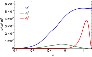
Figure 1: The left panel shows plot for $\sigma_{0}^{2}$, $\sigma_{2}^{2}$ and $\sigma_{d}^{2}$. On the right panel, blue curve is B-mode power spectrum for the standard weak lensing and red curve is for the weak lensing with the dipole distribution.

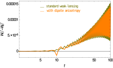
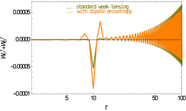
Figure 2: $W^{l^{\prime}}_{1l}-W^{l^{\prime}}_{2l}$ and $W^{l^{\prime}}_{1l}+W^{l^{\prime}}_{2l}$ are plotted with respect to $l^{\prime}$ for $l=10$ in the left and right panel respectively.

Table 1: fractional change in B-mode power spectrum from $l=20$ to $100$

“l”	20	40	60	80	100
$l(l+1)C_{Bl}/2\pi$ (standard lensing)	$0.000238658$	$0.00123632$	$0.002661348$	$0.004883204$	$0.00772255$
$l(l+1)C_{Bl}/2\pi$ (lensing with dipole anisotropy)	$0.000230123$	$0.0012477$	$0.002653185$	$0.004874728$	$0.007715724$
fractional change in $l(l+1)C_{Bl}/2\pi$	0.035762	0.0092	0.003067	0.001736	0.000884

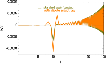
Figure 3: The plot of $W^{l^{\prime}}_{1l}$ with respect to $l^{\prime}$ for $l=10$.

We note that in Eq. (42), the modified power spectrums are determined by functions $W_{11}^{l^{\prime}}$, $W_{21}^{l^{\prime}}$ and $W_{31}^{l^{\prime}}$ those depend on $\sigma_{0T}^{2}$ and $\sigma_{2T}^{2}$. Since theoretically, the primordial $C_{\tilde{B}l}$ has nearly zero contribution, the correction to $C_{\tilde{E}l}$ is proportional to $W_{11}^{l^{\prime}}+W_{11}^{l^{\prime}}$ and the only contribution to $C_{Bl}$ comes from the correction which is proportional to $W_{11}^{l^{\prime}}-W_{11}^{l^{\prime}}$. In Fig. (1), on the left panel, we plot $\sigma_{0}^{2}$, $\sigma_{2}^{2}$ which are due to standard weak lensing. The function $\sigma_{d}^{2}$ due to dipole distribution is also plotted. We considered $\beta=1$ and $\kappa=0.046$ satisfying the constraint $|\kappa_{s}^{3}\beta|\leq 1.26\times 10^{-5}H_{0}^{3}$ or $|\kappa^{3}\beta|\leq 10^{-4}$Ghosh:2013blq , where, $H_{0}$ is Hubble constant. This provides with an estimate of maximum possible change that can arise due to the dipole. We observe a reasonable value of $\sigma_{d}^{2}$ comparable to $\sigma_{0}^{2}$. The contribution of $\sigma_{d}^{2}$ appears in the B-mode spectrum. Dipole distribution marginally decreases its value due to the presence of function $W_{11}^{l^{\prime}}-W_{11}^{l^{\prime}}$. In the right panel of Fig. (1), we plot the $B$-mode power spectrum including the dipole contribution. The standard weak lensing result is shown for comparison. In plotting the lensed $C_{Bl}$, we use unlensed $\tilde{C}_{Bl}=0$ and $\tilde{C}_{El}$ from CAMB package. We restrict this curve for $l>10$ for which the Flat sky approximation is expected to be reliable Hu:2000ee . We find that the dipole contribution leads to a small downward shift of the spectrum at low values of $l$. The shift is large at low $l$ and roughly 1% at $l$ of order 40. Hence it is small but not negligible. Some of the numerical values for B-mode power spectrum and corresponding fractional changes are given in Tab. (1). At higher values $l\geq 100$, the fraction change becomes below $0.1\%$. In Fig. (2), on the left panel, we note that $W_{11}^{l^{\prime}}-W_{11}^{l^{\prime}}$ is oscillatory and mainly lie in positive-value quadrant. Due to this asymmetry, dipole distribution could modify $C_{Bl}$. On other hand, $W_{11}^{l^{\prime}}+W_{11}^{l^{\prime}}$ is oscillatory as well as symmetric. Therefore, we do not get any contribution to the $C_{El}$ due to the dipole distribution. Similarly, $W_{11}^{l^{\prime}}$ forms a nearly symmetric pattern (see Fig. (3)) and it does not give any change to $C_{Tl}$ in the standard weak lensing modification due to dipole anisotropy.

V Conclusions

We generalized the formalism of weak lensing by adding dipole anisotropy in the Newtonian potential. We estimated the effect of lensing on the CMB power spectrum in this model. We followed the approach of the flat sky approximation. Weak lensing mixes E and B mode and hence we necessarily find some contribution to $C_{Bl}$ due to weak lensing. The correction to $C_{Bl}$ is proportional to $\tilde{C}_{El}$. We observed that adding dipole anisotropy changes $C_{Bl}$ for the lower range of $l$. However, dipole anisotropy does not lead to an appreciable change in $C_{El}$, since the correction is much smaller than the leading order term $\tilde{C}_{El}$. We did not even observe any change in the standard weak lensing modification due to the dipole anisotropy, since $W_{11}^{l^{\prime}}+W_{11}^{l^{\prime}}$ has a symmetric pattern. The same argument applies to $C_{Tl}$. In the case of $C_{Bl}$ we obtain a correction since in this case the leading order $\tilde{C}_{Bl}$ is zero and $W_{11}^{l^{\prime}}-W_{11}^{l^{\prime}}$ are not symmetric. For this case we computed the maximum possible correction to $C_{Bl}$ by fixing the direction of dipole to be same as the direction of observation. A more reliable calculation would use the spherical harmonics approach. Flat sky approximation and the spherical harmonics approach deviate below $l=10$ Hu:2000ee . Thus, our calculation is reliable for $l>10$, where we still find a small correction to $C_{Bl}$.

References

- (1) A. Lewis and A. Challinor, Phys. Rept. 429, 1 (2006) doi:10.1016/j.physrep.2006.03.002 [astro-ph/0601594].
- (2) C. L. Bennett et al. [WMAP Collaboration], Astrophys. J. Suppl. 208, 20 (2013) doi:10.1088/0067-0049/208/2/20 [arXiv:1212.5225 [astro-ph.CO]].
- (3) M. Tegmark, A. de Oliveira-Costa and A. Hamilton, Phys. Rev. D 68, 123523 (2003) doi:10.1103/PhysRevD.68.123523 [astro-ph/0302496].
- (4) C. J. Copi, D. Huterer and G. D. Starkman, Phys. Rev. D 70, 043515 (2004) doi:10.1103/PhysRevD.70.043515 [astro-ph/0310511].
- (5) K. Land and J. Magueijo, Phys. Rev. Lett. 95, 071301 (2005) doi:10.1103/PhysRevLett.95.071301 [astro-ph/0502237].
- (6) P. Vielva, E. Martinez-Gonzalez, R. B. Barreiro, J. L. Sanz and L. Cayon, Astrophys. J. 609, 22 (2004) doi:10.1086/421007 [astro-ph/0310273].
- (7) P. Mukherjee and Y. Wang, Astrophys. J. 613, 51 (2004) doi:10.1086/423021 [astro-ph/0402602].
- (8) M. Cruz, E. Martinez-Gonzalez, P. Vielva and L. Cayon, Mon. Not. Roy. Astron. Soc. 356, 29 (2005) doi:10.1111/j.1365-2966.2004.08419.x [astro-ph/0405341].
- (9) H. K. Eriksen, F. K. Hansen, A. J. Banday, K. M. Gorski and P. B. Lilje, Astrophys. J. 605, 14 (2004) Erratum: [Astrophys. J. 609, 1198 (2004)] doi:10.1086/382267 [astro-ph/0307507].
- (10) P. A. R. Ade et al. [Planck Collaboration], Astron. Astrophys. 571, A23 (2014) doi:10.1051/0004-6361/201321534 [arXiv:1303.5083 [astro-ph.CO]].
- (11) P. Jain and J. P. Ralston, Mod. Phys. Lett. A 14, 417 (1999) doi:10.1142/S0217732399000481 [astro-ph/9803164].
- (12) P. Jain, G. Narain and S. Sarala, Mon. Not. Roy. Astron. Soc. 347, 394 (2004) doi:10.1111/j.1365-2966.2004.07169.x [astro-ph/0301530].
- (13) J. P. Ralston and P. Jain, Int. J. Mod. Phys. D 13, 1857 (2004) doi:10.1142/S0218271804005948 [astro-ph/0311430].
- (14) C. Gordon, W. Hu, D. Huterer and T. M. Crawford, Phys. Rev. D 72, 103002 (2005) doi:10.1103/PhysRevD.72.103002 [astro-ph/0509301].
- (15) A. L. Erickcek, M. Kamionkowski and S. M. Carroll, Phys. Rev. D 78, 123520 (2008) doi:10.1103/PhysRevD.78.123520 [arXiv:0806.0377 [astro-ph]].
- (16) A. R. Liddle and M. Cortês, Phys. Rev. Lett. 111, no. 11, 111302 (2013) doi:10.1103/PhysRevLett.111.111302 [arXiv:1306.5698 [astro-ph.CO]].
- (17) S. Ghosh, Phys. Rev. D 89, 063518 (2014) doi:10.1103/PhysRevD.89.063518 [arXiv:1309.6547 [astro-ph.CO]].
- (18) R. Kothari, S. Ghosh, P. K. Rath, G. Kashyap and P. Jain, Mon. Not. Roy. Astron. Soc. 460, no. 2, 1577 (2016) doi:10.1093/mnras/stw1039 [arXiv:1503.08997 [astro-ph.CO]].
- (19) S. Ghosh, R. Kothari, P. Jain and P. K. Rath, JCAP 1601, no. 01, 046 (2016) doi:10.1088/1475-7516/2016/01/046 [arXiv:1507.04078 [astro-ph.CO]].
- (20) S. Ghosh and P. Jain, arXiv:1807.02359 [astro-ph.CO].
- (21) M. Zaldarriaga and U. Seljak, Phys. Rev. D 58, 023003 (1998) doi:10.1103/PhysRevD.58.023003 [astro-ph/9803150].
- (22) B. Yu and T. Lu, Astrophys. J. 698, 1771 (2009) doi:10.1088/0004-637X/698/2/1771 [arXiv:0903.4519 [astro-ph.CO]].
- (23) W. Hu, Phys. Rev. D 62, 043007 (2000) doi:10.1103/PhysRevD.62.043007 [astro-ph/0001303].