Zonal Jet Creation from Secondary Instability of Drift Waves for Plasma Edge Turbulence

Abstract

A new strategy is presented to explain the creation and persistence of zonal flows widely observed in plasma edge turbulence. The core physics in the edge regime of the magnetic-fusion tokamaks can be described qualitatively by the one-state modified Hasegawa-Mima (MHM) model, which creates enhanced zonal flows and more physically relevant features in comparison with the familiar Charney-Hasegawa-Mima (CHM) model for both plasma and geophysical flows. The generation mechanism of zonal jets is displayed from the secondary instability analysis via nonlinear interactions with a background base state. Strong exponential growth in the zonal modes is induced due to a non-zonal drift wave base state in the MHM model, while stabilizing damping effect is shown with a zonal flow base state. Together with the selective decay effect from the dissipation, the secondary instability offers a complete characterization of the convergence process to the purely zonal structure. Direct numerical simulations with and without dissipation are carried out to confirm the instability theory. It shows clearly the emergence of a dominant zonal flow from pure non-zonal drift waves with small perturbation in the initial configuration. In comparison, the CHM model does not create instability in the zonal modes and usually converges to homogeneous turbulence.

1 Introduction

Persistent zonal flows have been widely observed from the nature, experiments, and numerical simulations of various rotating fluids majda2003introduction ; pedlosky2013geophysical ; rhines1975waves ; lin1998 ; diamond2005zonal ; fujizawa2009 . In fusion plasma, poloidally extended zonal jets in the edge region of magnetically confined tokamak devices are of particular interest where the turbulent transport severely limits plasma confinement and leads to disastrous particle transport towards the boundary regime. The anomalous particle transport along the radial direction due to drift wave turbulence is found to be regulated and suppressed by the generation of poloidal zonal structures hortonreview1999 ; diamond2005zonal ; majda2018flux ; xanthopoulos2011 ; pushkarev2013 . It has been suggested from several theoretical and numerical results smolyakov2000coherent ; manfredi2001zonal that zonal flows are generated spontaneously by interacting with the drift waves. The drift wave in plasma edge turbulence is also analogous to the Rossby wave in geostrophic fluids where similar zonal jet structures are observed majda2003introduction ; dewar2007zonal .

In understanding the drift wave – zonal flow interacting dynamics, it is useful to adopt simplified models where the most relevant physical mechanism is identified. The Hasegawa-Mima (HM) hasegawa1978pseudo ; dewar2007zonal and Hasegawa-Wakatani (HW) hasegawa1983plasma ; numata2007bifurcation models are two groups of the simplified models which are capable to qualitatively capture the energy-conserving nonlinear dynamics for the formation of zonal jets. The HM models contain most essential physical features in the drift wave – zonal flow feedback loop mechanism, while the HW models include a drift wave instability driving the turbulence. Striking new features are generated in a newly developed flux-balanced Hasegawa-Wakatani (BHW) model majda2018flux ; 2018arXiv181200131Q , where corrected treatment for the electron responses parallel to the magnetic field lines is introduced as a more physical improvement from the modified Hasegawa-Wakatani (MHW) model hasegawa1983plasma ; numata2007bifurcation . One important observation from the BHW model simulations is the enhanced stronger zonal jets persistent in all the dynamical regimes even with high particle resistivity 2018arXiv181200131Q ; majda2018flux . In contrast, the MHW model lacks the skill to maintain such strong zonal jets and ceases to homogeneous drift wave turbulence at the low resistivity limit.

In analyzing zonal flows from drift wave turbulence, the BHW model consists of the interplay of the linear drift wave instability and the nonlinear coupling between drift waves and zonal states. The modified Hasegawa-Mima (MHM) model, as the exact adiabatic one-state limit majda2018flux of the BHW model, gives a cleaner setup by filtering out the linear instability, thus offers a more desirable starting model for investigating the central mechanism in flow self-organization from drift waves to coherent zonal states through nonlinear interactions. The MHM model is modified from the original Charney-Hasegawa-Mima (CHM) model hasegawa1978pseudo for plasma and geophysical flows which is also known as the quasi-geostrophic model dewar2007zonal ; majda2003introduction . Modulational instability of drift waves offers a feedback mechanism for the generation of zonal flows through the nonlinear interactions. Theories and numerical experiments have been attempted manfredi2001zonal ; smolyakov2000coherent ; manz2013 for describing the emergence of zonal flows by Reynolds stress in both CHM and MHM models.

In this paper, we provide a precise explanation for the underlying mechanism in creating the dominant zonal jets observed in the flux-balanced models using secondary instability analysis about a background base state of drift wave solutions. To identify the important nonlinear impact between interactions of the drift wave states and the zonal modes, we stay in the simple one-state Hasegawa-Mima (HM) models at the adiabatic limit of the two-state BHW model, where no internal instability due to the particle resistivity is included to add extra complexity in the flow turbulence. The generation and persistence of zonal flows in the HMH model is investigated by demonstrating that: first a non-zonal drift wave base state induces strong instability in the zonal modes, implying nonlinear energy transfer to the zonal states; and then the generated zonal structure as a base state stays stable to perturbations thus is maintained in time as the system evolves. The secondary instability results are first illustrated by numerical computation of the largest growth exponent from the Floquet theory. Further, we use direct numerical simulations to confirm the jet creation mechanism. Zonal flows are induced from a pure drift wave state adding small isotropic fluctuations in the MHM model even without any dissipation effect. In the case with dissipation, selective decay principle developed in qi2018selective helps to work together with the secondary instability mechanism to drive the state to a final purely zonal structure. In contrast in the CHM model, none of these instability and zonal jets are created due to the improper treatment in the electron flux response.

In the structure of this paper, we first briefly describe the BHM and MHM models with a balanced averaged flux creating strong zonal jets. Section 2 introduces the basic MHM model properties with its major physical interpretation. The exact single mode drift wave solution as well as the zonal mean dynamics is derived in Section 3 for the background base mode in generating the zonal states. The precise energy transfer mechanism to the zonal modes is explained through the secondary instability about the background state with numerical computations of the growth rate in Section 4. Section 5 uses direction numerical simulations with and without dissipation effects for confirming the developed theories. The conclusion and further discussion are given in the final Section 6.

1.1 The flux balanced models for plasma edge turbulence

In tokamak devices, the realistic geometry would be a circular domain with a predominant magnetic field $\mathbf{B}$ along the toroidal $z$-direction. However, the shape of the plasma edge can be approximated on a slab geometry under a Cartesian coordinate where the toroidal magnetic surfaces are embedded. The Hasegawa-Wakatani models describe the drift wave – zonal flow interactions of a two state coupled system on the 2D slab geometry majda2018flux ; dewar2007zonal , with $x$-axis corresponding to the radial direction and $y$-axis representing the poloidal direction. The flux-balanced Hasegawa-Wakatani (BHW) model is introduced in majda2018flux based on the flux-balanced potential vorticity $q=\nabla^{2}\varphi-\tilde{n}$ and the density fluctuation $n$ in the following form

$$\frac{\partial q}{\partial t}+\nabla^{\bot}\varphi\cdot\nabla q-\kappa\frac{\partial\varphi}{\partial y} = D\Delta q,\quad q=\nabla^{2}\varphi-\tilde{n},$$ (1a)

$$\frac{\partial n}{\partial t}+\nabla^{\bot}\varphi\cdot\nabla n+\kappa\frac{\partial\varphi}{\partial y} = \alpha\left(\tilde{\varphi}-\tilde{n}\right)+D\Delta n,$$ (1b)

where $\varphi$ is the electrostatic potential, $n$ is the density fluctuation from background density $n_{0}\left(x\right)$, and $\mathbf{u}\equiv\nabla^{\bot}\varphi=\left(-\partial_{y}\varphi,\partial_{x}\varphi\right)$ is the velocity field. The parameter $\alpha$ is for adiabatic resistivity of parallel electrons. It determines the degree to which electrons can move rapidly along the magnetic field lines. The constant background density gradient $\kappa=-\nabla\ln n_{0}$ is defined by the exponential background density profile near the boundary $n_{0}\left(x\right)$ . $D$ acts on the two states with the Laplace operator as a homogeneous damping 2018arXiv181200131Q ; majda2018flux . The physical quantities $\varphi$ and $n$ are decomposed into zonal mean stats $\overline{\varphi},\overline{n}$ and their fluctuations about the mean $\tilde{\varphi},\tilde{n}$ so that

$$\varphi=\overline{\varphi}+\tilde{\varphi},\;n=\overline{n}+\tilde{n},\quad\overline{f}\left(x\right)=L_{y}^{-1}\int f\left(x,y\right)dy.$$

In the BHW model, the poloidally averaged density $\overline{n}$ along $y$-direction is removed from the potential vorticity $q$. In contrast, the original Hasegawa-Wakatani model introduced in hasegawa1983plasma as well as the modified version (MHW) numata2007bifurcation uses the ‘unbalanced’ potential density $q=\nabla^{2}\varphi-n$ without removing the mean state $\overline{n}$ in the potential vorticity, leading to problems with the convergence at the adiabatic limit $\alpha\rightarrow\infty$.

The BHW model offers a more realistic formulation with several desirable properties. Most importantly, it is shown from rigorous proof and numerical confirmation majda2018flux ; 2018arXiv181200131Q that at the adiabatic limit, $\alpha\rightarrow\infty$, the BHW model converges to the following equation

$$\frac{\partial q}{\partial t}+\nabla^{\bot}\varphi\cdot\nabla q-\kappa\frac{\partial\varphi}{\partial y}=D\Delta q,\quad q=\nabla^{2}\varphi-\tilde{\varphi},$$ (2)

which is called the modified Hasegawa-Mima model. Notice the modification by removing zonal state in $\tilde{\varphi}$ in the definition of potential vorticity $q$ above. On the other hand, the MHW model shows performance significantly different from the MHM model when $\alpha\rightarrow\infty$. The strong zonal jets created from the BHW and MHM model and the convergence at the adiabatic limit are discussed with explicit numerical simulations in majda2018flux (see Fig. 4 and 5 there). If we replace the potential vorticity in (2) by $q=\nabla^{2}\varphi-\varphi$ without removing the zonal mean state, it recovers the Charney-Hasegawa-Mima model. The CHM model is identical to the quasi-geostrophic model with $F$-plane effect describing geophysical turbulence with rotation and stratification majda2003introduction ; pedlosky2013geophysical ; qi2016low . Then the rigorous theories developed for the geophysical model apply to the CHM model exactly in the same way. In this paper, we will focus on the HM models and especially changes in MHM model due to the averaged flux correction in order to analyze the unstable effect purely from a background base flow.

2 The Hasegawa-Mima models and their representing properties

To offer a better illustration with physical interpretations in the Hasegawa-Mima models, we start with the original dimensional formulation with physically related variables and derive the non-dimensionalized version using the physical scales. The Charney-Hasegawa-Mima (CHM) equation and the modified Hasegawa-Mima (MHM) equation can be formulated under the same framework by defining a switch parameter with $s=0$ for CHM and $s=1$ for MHM as

$$\frac{D}{Dt}\left(\frac{\zeta}{\omega_{\mathrm{ci}}}+\ln\frac{\omega_{\mathrm{ci}}}{n_{0}}-\frac{e}{T_{e}}\left(\tilde{\varphi}+\delta_{s0}\overline{\varphi}\right)\right)=0,$$ (3)

where $\varphi$ is the electrostatic potential, $\zeta=\nabla^{2}\varphi/B_{0}$ is the vorticity, $\mathbf{v}_{E}=-\nabla\varphi\times\hat{z}/B_{0}$ is the $\mathbf{E\times B}$ velocity. $D/Dt\equiv\partial_{t}+\mathbf{v}_{E}\cdot\nabla$ represents the material derivative along the velocity. In the parameters, $T_{e}$ is the reference electron temperature, $\omega_{\mathrm{ci}}=eB_{0}/m_{i}$ is the ion cyclotron frequency, and $m_{i}$ is the ion mass dewar2007zonal . For model non-dimensionalization, the new variables are introduced by

$$e\varphi/T_{e}\rightarrow\varphi,\quad\omega_{\mathrm{ci}}t\rightarrow t,\quad\left(x,y\right)/\rho_{s}\rightarrow\left(x,y\right),$$

with $\rho_{s}=\omega_{\mathrm{ci}}^{-1}\left(T_{e}/m_{i}\right)^{1/2}=\sqrt{m_{i}T_{e}}/eB_{0}$ the characteristic length scale of drift waves and $\omega_{\mathrm{ci}}^{-1}$ the characteristic time scale from the ion frequency. Accordingly, we find the non-dimensional velocity and vorticity

$$\rho_{s}\frac{eB_{0}}{T_{e}}\mathbf{v}_{E}\rightarrow\mathbf{v}_{E}=\nabla^{\bot}\varphi,\quad\rho_{s}^{2}\frac{eB_{0}}{T_{e}}\zeta\rightarrow\zeta.$$

By substituting the non-dimensionalized quantities back into the dimensional equation (3), we can rewrite the original (with $s=0$) and modified (with $s=1$) Hasegawa-Mima equations in the non-dimensional form as in (2) so that

$$\left(\frac{\partial}{\partial t}+\nabla^{\bot}\varphi\cdot\nabla\right)q+\left(\partial_{x}\ln n_{0}\right)\frac{\partial}{\partial y}\tilde{\varphi}=0,\quad q=\zeta-\left(\tilde{\varphi}+\delta_{s0}\overline{\varphi}\right).$$ (4)

Above we introduce the new variable $q$ as the potential vorticity, and if we assume a constant exponential decay profile in the background density $n_{0}\sim\exp\left(-\kappa x\right)$ the coefficient becomes a constant $\kappa\equiv-\partial_{x}\ln n_{0}$.

On the magnetic surfaces, the electrons are assumed to respond adiabatically so that locally thermodynamical equilibrium (with Boltzmann distribution) is achieved on a given field surface. The electron density fluctuation does not respond adiabatically on the averaged part of the electrostatic potential $\overline{\varphi}$, thus only the flux balanced component $e\tilde{\varphi}/T_{e}$ follows the Boltzmann distribution. This offers the intuition for removing the zonal mean state $\overline{\varphi}$ in the MHM model. Though simple enough, the modified expansion leads to much stronger zonal jet structures and more physically consistent performance dewar2007zonal ; manfredi2001zonal compared with the CHM results.

2.1 Galilean invariance and model energetics

We illustrate some representative features especially from the model flux modification. First, the MHM model enhances the excitation of zonal flows with more prominent zonal structures. Consider a single mode plane wave $\varphi=A_{z}\left(x,t\right)\exp\left(i\left(\mathbf{k\cdot x}-\omega t\right)\right)$ decomposed into a slowly varying zonal mean and fast fluctuation. The slow mode $A_{z}$ is assumed to be zonal and gives a constant zonal mean flow $\mathbf{v}_{E}=\bar{v}\hat{y}$. We can find the linearized dispersion relations for CHM and MHM separately as

$$\mathrm{CHM:\quad} \omega=\frac{k_{y}\kappa}{1+k^{2}}+\frac{k^{2}}{1+k^{2}}k_{y}\overline{v},$$

$$\mathrm{MHM:\quad} \omega=\frac{k_{y}\kappa}{1+k^{2}}+k_{y}\overline{v}.$$

Without the mean flow $\mathbf{v}_{E}$, the HM models generate no instability with the same dispersion relation in the first term on the right side. In small scales $k\gg 1$, the CHM and MHM models have similar dispersion relations. In large scales $k\lesssim 1$ (that is, near the scale of $\rho_{s}$), the modified model gets a stronger feedback from the fluctuation (due to the simple Doppler shift $\mathbf{k\cdot v}_{E}=k_{y}\bar{v}$). In the unmodified model, the Doppler shift is reduced by a factor $k^{2}/\left(1+k^{2}\right)$. Detailed discussions about mean flow interaction in the CHM model can be found in majda2003introduction .

Second, the MHM model is Galilean invariant under boosts in the $y$ (poloidal) direction as desired for the symmetry in the poloidal direction of tokamak devices. If we introduce a poloidal boost $V$ in the flow, the new states become

$$y^{\prime}=y-Vt,\quad\varphi^{\prime}=\varphi-VB_{0}x.$$

Notice that only the fluctuation in the electrostatic potential is invariant, $\tilde{\varphi}^{\prime}=\tilde{\varphi}$, while the zonal mean is not invariant, $\overline{\varphi}^{\prime}=\overline{\varphi}-VB_{0}x$, under the change of coordinate. The CHM model (and also the QG model in geophysics) does not maintain this invariance due to the last term $e\overline{\varphi}/T_{e}$ with $s=0$.

At last, we describe the model energetics. In the MHM model, two important conserved quantities qi2018selective ; numata2007bifurcation can be found as the energy $E$ and the enstrophy $W$

$$E=\frac{1}{2}\int\tilde{\varphi}^{2}+\left|\nabla\varphi\right|^{2},\quad W=\frac{1}{2}\int q^{2}=\frac{1}{2}\int\left(\tilde{\varphi}-\nabla^{2}\varphi\right)^{2}.$$ (5)

The nonlinear term in (4) does not alter the value of both energy and enstrophy. Thus the evolution of energy and enstrophy can be purely determined by the dissipation effects. Especially with the homogeneous damping form $D\Delta q$ in (2), we can derive the dynamical equations

$$\frac{dE}{dt}= -D\int\left|\nabla\tilde{\varphi}\right|^{2}+\left|\nabla^{2}\varphi\right|^{2},$$

$$\frac{dW}{dt}= -D\int\left|\nabla q\right|^{2}=-D\int\left|\nabla\tilde{\varphi}\right|^{2}+2\left|\nabla^{2}\varphi\right|^{2}+\left|\nabla^{3}\varphi\right|^{2}.$$

Similarly, the CHM model also maintains two invariants with $\tilde{\varphi}$ in the definition (5) and equations replaced by $\varphi$. The energetic equations play important roles in showing the stability and decay properties. In particular, a selective decay to a single dominant mode can be discovered based on the energetics majda2000selective ; qi2018selective .

2.2 Selective decay in the flux balanced model

The persistence of the zonal jets in the MHM model can be first explained in a rigorous mathematical approach using the selective decay principle qi2018selective ; majda2000selective . It states that proper dissipation operator can dissipate all the non-zero drift wave states at a much faster rate except a single selected dominant zonal state in the MHM model. Precisely speaking, we have the convergence to one of the selective decay zonal states $\overline{\varphi}_{k}$ for the normalized potential function in the $H^{1}$ sense

$$\lim_{t\rightarrow\infty}\left\|\nabla\phi-\nabla\overline{\phi}_{k}\right\|_{0}=0,\quad\phi=\frac{\varphi}{\left\|\nabla\varphi\right\|_{0}}.$$ (6)

In the CHM model, the selective decay state $\varphi_{k}$ in a single wavenumber can be also reached under the dissipation operator, while the final converged state is one drift wave mode without zonal structure. Proof for the selective decay results using different dissipation operators including the Landau damping with detailed numerical simulations are shown in qi2018selective . Still, the generation of the zonal structures from any arbitrary initial states is directly related with the nonlinear interaction mechanism between different modes before the selective decay effect takes over.

3 Exact drift wave solutions and the zonal mean dynamics

Now we propose the precise model framework for analyzing the instability, creation and stabilization of zonal jets through the nonlinear interacting mechanism with the background base states. First, we introduce additional rescaling for the HM models so that the important parameters that determine the solution structures are identified. Starting with the previous model formulation (4)

$$\frac{\partial q}{\partial t}+\nabla^{\bot}\varphi\cdot\nabla q-\kappa\frac{\partial\varphi}{\partial y}=D\Delta q,\quad q=\nabla^{2}\varphi-\left(\tilde{\varphi}+\delta_{s0}\overline{\varphi}\right),$$

with $s=1$ for the MHM model and $s=0$ for the CHM model, we propose the rescaled set of variables $\left(q^{\prime},\varphi^{\prime},\mathbf{x}^{\prime},t^{\prime}\right)$ based on the characteristic length scale $L$ and the characteristic flow velocity scale $U$

$$\mathbf{x}=L\mathbf{x}^{\prime},\;\mathbf{u}=\nabla^{\bot}\varphi=U\mathbf{u}^{\prime},\quad t=Tt^{\prime},\;\varphi=\Phi\varphi^{\prime},\;q=Qq^{\prime}.$$

The scales of the other variables can be found based on the values of $L,U$ as

$$T=\frac{L}{U},\;\Phi=UL,\;Q=\frac{\Phi}{L^{2}}=\frac{U}{L}.$$

With the above rescaling, the unit wavenumber mode $\mathbf{p},\left|\mathbf{p}\right|=1$ for the new state represents the inverse length scale $L^{-1}$, and the flow state with unit amplitude $u=\exp\left(\mathbf{p\cdot x}\right)$ represents the velocity with strength $U$. Accordingly, we derive the rescaled HM models for the normalized states $\left(q^{\prime},\varphi^{\prime},\mathbf{x}^{\prime},t^{\prime}\right)$ based on the proposed characteristic scales

$$\frac{\partial q^{\prime}}{\partial t^{\prime}}+\nabla_{\mathbf{x}^{\prime}}^{\bot}\varphi^{\prime}\cdot\nabla_{\mathbf{x}^{\prime}}q^{\prime}-\kappa^{\prime}\frac{\partial\varphi^{\prime}}{\partial y^{\prime}}=D^{\prime}\Delta_{\mathbf{x}^{\prime}}q^{\prime},\quad q^{\prime}=\nabla_{\mathbf{x}^{\prime}}^{2}\varphi^{\prime}-L^{2}\left(\tilde{\varphi}^{\prime}+\delta_{s0}\overline{\varphi}^{\prime}\right).$$ (7)

The above rescaled equation (7) is not changed much just with new non-dimensional parameters $\kappa^{\prime},D^{\prime}$. Notice that the length scale $L$ now appears explicitly in the potential vorticity $q^{\prime}$. The flow solution is entirely determined by the two characteristic coefficients, $\kappa^{\prime}=\frac{\kappa L^{2}}{U}$ and $D^{\prime}=\frac{D}{UL}$. $\kappa^{\prime}$ has the same role as the Rhines number $\mathrm{Rh}^{-1}$ in geophysical flows, showing the anisotropic effect in the drift waves; and $D^{\prime}$ as the Reynolds number $\mathrm{Re}^{-1}$ for the dissipation effect rhines1975waves ; pedlosky2013geophysical . We will focus on the MHM model with $s=1$ in (7) and neglect the primes on the states in the rest part of the paper (the CHM case can be easily implied and detailed theories for the CHM model have actually been developed in the geophysical literatures majda2003introduction ; majda2016introduction ; majda2018strategies ).

3.1 General base flow state from the exact solution

Exact drift wave solutions of the MHM equation in (7) can be found by considering a single mode base state. We assume the base mode in the electrostatic potential and the potential vorticity for a single wavenumber $\mathbf{k}=\left(k^{x},k^{y}\right)$ as

$$\varphi\left(\mathbf{x},t\right)=\hat{\varphi}\exp\left(i\left(\mathbf{k\cdot x}-\omega\left(\mathbf{k}\right)t\right)\right),\quad q\left(\mathbf{x},t\right)=-\left[k^{2}+L^{2}\left(1-\delta_{k^{y},0}\right)\right]\hat{\varphi}\exp\left(i\left(\mathbf{k\cdot x}-\omega\left(\mathbf{k}\right)t\right)\right),$$ (8)

where $\omega\left(\mathbf{k}\right)$ is the dispersion relation in the drift waves. The Kronecker delta operator is introduced for the MHM model modification in the zonal modes $k^{y}=0$. The normalized wavenumber length $k=\left|\mathbf{k}\right|$ is compared with the characteristic scale $L$, i.e., wavenumbers $k<1$ characterize the scales larger than $L$ and wavenumbers $k>1$ for scales smaller than $L$. Since we only consider a single mode solution in the above form, the nonlinear term $\nabla^{\bot}\varphi\cdot\nabla q$ vanishes in the equation through the self interaction $\mathbf{k}^{\bot}\cdot\mathbf{k}=0$. The dispersion relation can be found as

$$\omega\left(\mathbf{k}\right)=\kappa^{\prime}\frac{k^{y}}{k^{2}+L^{2}},\quad\kappa^{\prime}=\frac{\kappa L^{2}}{U}.$$ (9)

Notice that the above dispersion relation $\omega\left(\mathbf{k}\right)$ is valid for both the MHM and CHM models. In fact, the MHM model only adds modifications for the zonal modes with $k^{y}=0$. In the zonal modes, the dispersion relation becomes $\omega=\kappa^{\prime}k^{y}/k^{2}=0$. The formula (9) is still valid for both the MHM ($s=1$) case and CHM ($s=0$) case. Next, we will consider the instability of fluctuation perturbations added on top of the representative exact solutions in the form of (8).

3.2 Dynamical equation of the zonal mean state

Before proceeding to the detailed discussion about secondary instability to induce zonal structures, it is useful to check the exact dynamical equation for the zonal state to achieve a first intuition about the nonlinear interacting mechanism. Evolutions of the zonal components $\overline{q}$ can be extracted from the above MHM model by directly taking the zonal average about the original equation (7)

$$\frac{\partial\overline{q}}{\partial t}+\frac{\partial}{\partial x}\overline{uq}=-D^{\prime}\frac{\partial^{4}\overline{q}}{\partial x^{4}},\quad u=-\partial_{y}\varphi,$$ (10)

with $u$ the zonal velocity fluctuation. The background density gradient term $\kappa^{\prime}\partial_{y}\varphi$ vanishes after the average along $y$-direction. If there is no non-zero zonal mode $k^{y}=0$, we can check that the advection term vanishes

$$\overline{uq}=\overline{\left(-ik^{y}\hat{\varphi}e^{i\left(\mathbf{k\cdot x}-\omega t\right)}\right)\left(-\left(k^{2}+L^{2}\right)\hat{\varphi}e^{i\left(\mathbf{k\cdot x}-\omega t\right)}\right)+c.c.}=\overline{ik^{y}\left(k^{2}+L^{2}\right)\hat{\varphi}^{2}e^{2i\left(\mathbf{k\cdot x}-\omega t\right)}+c.c.}=0,$$

after the integration along the $y$-direction, with $c.c.$ as the complex conjugate part. Therefore single non-zonal fluctuation mode makes no contribution to the zonal mean structure in the above form, where an exact solution (8) can be reached.

On the other hand, zonal wave could be generated through the interactions between different wavenumbers. If we consider a general solution with multiple drift wave modes, the mean state equation can be derived in the following form

$$\left(\frac{d}{dt}+Dk^{2}\right)\overline{\varphi}_{\mathbf{k}}\left(t\right)=k^{-2}\sum_{\mathbf{m+n=k}}C_{\mathbf{kmn}}\left(t\right)\left(n^{2}-m^{2}\right)\overline{\varphi_{\mathbf{m}}\varphi_{\mathbf{n}}},$$

with the zonal mode $\mathbf{k}=\left(k^{x},0\right)$ and the fluctuation feedback $\overline{\varphi_{\mathbf{m}}\varphi_{\mathbf{n}}}$, $m^{y}\neq 0,n^{y}\neq 0$ to the zonal state. The coupling parameter $C_{\mathbf{kmn}}\left(t\right)$ is time-dependent on the dispersion relations (9) and models the triad coupling between the interacting drift wave modes

$$C_{\mathbf{kmn}}\left(t\right)=k^{x}n^{x}e^{i\left(\omega\left(\mathbf{k}\right)-\omega\left(\mathbf{m}\right)-\omega\left(\mathbf{n}\right)\right)t},\quad m^{x}+n^{x}=k^{x},\;m^{y}+n^{y}=0.$$

The right hand side of the above equation describes the nonlinear flux to the mean mode for the generation of a zonal jet. In the next section, we illustrate in a rigorous way how this nonlinear coupling term transfers the fluctuating energy in the non-zonal drift wave modes to the zonal directions, and maintains the zonal structures through the secondary stability mechanism.

4 Secondary instability from a base flow state

In this section, we provide a precise description for the energy transfer mechanism from the drift wave states (with $k^{y}\neq 0$) to zonal flows (with $k^{y}=0$). From the discussion in the last section, energy in the fluctuation drift wave modes is first transferred to the zonal directions through the resonant triad interactions; next the accumulation of energy in the zonal modes gets saturated and stabilized with the large-scale stability of a zonal base state. The drift wave – zonal flow interactions are characterized by the secondary instability analysis based on a base flow state. A brief summary for the main result achieved for the MHM model is: a fluctuation drift wave base state will induce strong instability along a wide range of zonal modes, implying strong transport of energy from non-zero drift waves to the zonal directions; in contrast a purely zonal flow base state will add no instability to zonal modes or the drift waves, showing stability in the generated zonal mean structure.

4.1 Formulation of the secondary instability from a base state

First notice that drift wave instability is filtered out in the one-state Hasegawa-Mima models (7), which enables us to focus on the nonlinear interaction mechanism from a background state. Below we derive the secondary instability based on the MHM model (the CHM case can be derived in a similar fashion). The development is motivated by the secondary instability analysis carried out in lee2003stability for geophysical turbulence on beta-plane and in meshalkin1962investigation for 2D Navier-Stokes equations with a Kolmogorov base flow using Floquet theory. However, the main focus here is the changes introduced through the flux modification in the MHM model potential vorticity $q=\nabla^{2}\varphi-\tilde{\varphi}$.

For simplicity in the MHM model, we consider a single mode base state with wavevector $\mathbf{p}=\left(\cos\theta_{p},\sin\theta_{p}\right)$ of unit length (then $\theta_{p}$ defines the characteristic direction of the base flow with $\theta_{p}=0$ for the zonal flow state and $\theta_{p}=\frac{\pi}{2}$ for the pure drift wave state). The single mode base flow potential $\varPhi_{p}$ and vorticity $Q_{p}=\nabla^{2}\varPhi_{p}-L^{2}\tilde{\varPhi}_{p}$ with the unit length wavenumber $\mathbf{p}$ can be defined from the exact solution formula (8) as

$$\varPhi_{p}=-\frac{1}{2}e^{i\left(\mathbf{p\cdot x}-\omega\left(\mathbf{p}\right)t\right)}-\frac{1}{2}e^{-i\left(\mathbf{p\cdot x}-\omega\left(\mathbf{p}\right)t\right)},\quad Q_{p}=-\left[1+L^{2}\left(1-\delta_{p^{y},0}\right)\right]\varPhi_{p},$$ (11)

with the dispersion relation $\omega\left(\mathbf{p}\right)=\kappa^{\prime}\frac{p^{y}}{1+L^{2}}$ defined in (9). From the rescaled equation (7) using the characteristic scales $\left(L,U\right)$, the base solution $U_{p}=\nabla^{\bot}\varPhi_{p}$ with unit wavenumber $p=1$ represents the characteristic length scale $L$ and the characteristic flow velocity $U$. For the corresponding CHM model solution, we just need to remove the delta functions in the above formula. With no additional internal instability in the HM models, the above solution can be simply generated by a combined forcing and damping effect.

The Floquet theory considers a fluctuation solution with a characteristic multiplier $e^{\mu t}$. To study the secondary instability at each wavenumber $\mathbf{k}$ based on the single-mode base flow (11), we introduce fluctuations, $\varphi_{p}=\varphi-\varPhi_{p}$, $q_{p}=q-Q_{p}$, on top of the base state in the form

$$\varphi_{p}= e^{\mu t}e^{i\left(\mathbf{k\cdot x}-\omega\left(\mathbf{k}\right)t\right)}\sum_{l=-N}^{N}\hat{\varphi}_{l}e^{il\left(\mathbf{p}\cdot\mathbf{x}-\omega\left(\mathbf{p}\right)t\right)},$$ (12)

$$q_{p}= e^{\mu t}e^{i\left(\mathbf{k\cdot x}-\omega\left(\mathbf{k}\right)t\right)}\sum_{l=-N}^{N}-\left[q^{2}\left(l\right)+L^{2}\left(1-\delta_{q^{y},0}\right)\right]\hat{\varphi}_{l}e^{il\left(\mathbf{p}\cdot\mathbf{x}-\omega\left(\mathbf{p}\right)t\right)}.$$

The perturbation is added on the wavenumber $\mathbf{k}$ with dispersion relation $\omega\left(\mathbf{k}\right)$. $\mu$ is the Floquet exponent characterizing the growth or decay rate in this perturbed mode. $\mathbf{q}\left(l\right)=\mathbf{k}+l\mathbf{p}$ with $q^{2}\left(l\right)=\left|\mathbf{q}\left(l\right)\right|^{2}$ is the full wavenumber with the perturbation. The perturbation mode $\hat{\varphi}_{l}$ is added on each of the directions as multiples of the characteristic wavenumber $l\mathbf{p}$ . It refers to a multiplicative perturbation along the directions of the base state flow. Here we truncate the perturbed states within the leading modes up to $N$ multiples of the base state. Thus the perturbation coefficients $\left\{\hat{\varphi}_{l}\right\}$ form a finite dimensional system of $2N+1$ real states. The problem can be further extended to an infinite dimensional system as the truncation size $N\rightarrow\infty$. Still, since we are mostly interested in the instability among the largest scales in the zonal states, a finite size truncation $N$ will be sufficient for characterizing this instability (see the instability results illustrated in Section 4.2).

By subtracting the base flow solution $\left(\varPhi_{p},Q_{p}\right)$ from the MHM equation (7), the fluctuation equation for the perturbed component $q_{p}$ of potential vorticity can be derived in the following form

$$\frac{\partial q_{p}}{\partial t}+\nabla^{\bot}\varPhi_{p}\cdot\nabla\left[q_{p}+\varphi_{p}+L^{2}\left(1-\delta_{p^{y},0}\right)\varphi_{p}\right]+\nabla^{\bot}\varphi_{p}\cdot\nabla q_{p}-\kappa^{\prime}\frac{\partial\varphi_{p}}{\partial y}=D^{\prime}\Delta q_{p},\;q_{p}=\nabla^{2}\varphi_{p}-\tilde{\varphi}_{p},$$

where the relation for the single mode base state vorticity and potential, $Q_{p}=-\left[1+L^{2}\left(1-\delta_{p^{y},0}\right)\right]\varPhi_{p}$, is used. Still in the secondary stability analysis, we focus on the secondary instability induced by the interactions between the background base state $\left(\varPhi_{p},Q_{p}\right)$ and the fluctuation modes $\left(\varphi_{p},q_{p}\right)$ with small perturbations. The higher-order nonlinear term between fluctuation modes, $\nabla^{\bot}\varphi_{p}\cdot\nabla q_{p}$, is assumed to stay small in the starting transient state and is neglected in this instability analysis. The unstable growth in perturbations due to the background base state is represented by the growth parameter $\mu$ in the fluctuation states (12). With a positive value in the real part of $\mu$, it infers exponential growth of the perturbation mode in the transient state on top of the base mode due to the interactions. The equation for calculating the secondary growth $\mu$ can be achieved by substituting the fluctuation modes (12) into the above fluctuation equation for $q_{p}$. It becomes an eigenvalue problem for each perturbation direction $\mathbf{k}$ individually with interactions between the triad neighboring modes $\left(\hat{\varphi}_{l-1},\hat{\varphi}_{l},\hat{\varphi}_{l+1}\right)$

$$\begin{aligned} \left[\mu\left(\mathbf{k}\right)-i\omega\left(\mathbf{k}\right)-il\omega\left(\mathbf{p}\right)+i\omega\left(\mathbf{q}\left(l\right)\right)+Dq^{2}\left(l\right)\right]\hat{\varphi}_{l}\\ +\frac{1}{2q^{2}\left(l\right)}\left(\mathbf{p\times k}\right)\cdot\hat{z}\left[q^{2}\left(l-1\right)-1-L^{2}\left(1-\delta_{p^{y},0}\right)\right]\hat{\varphi}_{l-1}\\ -\frac{1}{2q^{2}\left(l\right)}\left(\mathbf{p\times k}\right)\cdot\hat{z}\left[q^{2}\left(l+1\right)-1-L^{2}\left(1-\delta_{p^{y},0}\right)\right]\hat{\varphi}_{l+1}\end{aligned}=0,\;l=-N,\cdots,N.$$ (13)

with the combined wavenumber $\mathbf{q}\left(l\right)=\mathbf{k}+l\mathbf{p}$, $q^{2}\left(l\right)=\left|\mathbf{q}\left(l\right)\right|^{2}$, and the coupling coefficient $\left(\mathbf{p\times k}\right)\cdot\hat{z}=p^{x}k^{y}-p^{y}k^{x}$. The first row above includes the effects from the dispersion relation and damping, and the second and third rows are due to the interactions with the neighboring modes through the background state. The equations in (13) form a $\left(2N+1\right)\times\left(2N+1\right)$ tri-diagonal system (with $N$ the number of base mode perturbations added) based on the perturbed modes $\hat{\varphi}_{l}$ for each wavenumber $\mathbf{k}$. The solution of $\mu$ reflecting instability can be achieved by computing the eigenvalues of the corresponding tri-diagonal matrix. The maximum positive eigenvalue in real part of $\mu^{\mathrm{max}}\left(\mathbf{k}\right)$ refers to the most unstable growth rate in the mode $\mathbf{k}$ according to the base flow in direction $\mathbf{p}$.

As a comment for the general case, the base flow can be generalized to a combination of the single drift wave solutions (8) with a group of characteristic wavevectors $\left\{\mathbf{p}_{j}\right\}_{j=1}^{J}$. The base states for the electrostatic potential $\varPhi$ and the potential vorticity $Q=\nabla^{2}\varPhi-L^{2}\tilde{\varPhi}$ then can be defined as the combination of all the modes

$$\varPhi\left(\mathbf{x},t;\left\{\mathbf{p}_{j}\right\}_{j=1}^{J}\right)=\sum_{j=1}^{J}A_{j}e^{i\left(\mathbf{p}_{j}\cdot\mathbf{x}-\omega\left(\mathbf{p}_{j}\right)\right)},\;Q\left(\mathbf{x},t;\left\{\mathbf{p}_{j}\right\}_{j=1}^{J}\right)=-\sum_{j=1}^{J}A_{j}\left[p_{j}^{2}+L^{2}\left(1-\delta_{p_{j,0}^{y}}\right)\right]e^{i\left(\mathbf{p}_{j}\cdot\mathbf{x}-\omega\left(\mathbf{p}_{j}\right)\right)}.$$

Above $J$ is the total number of characteristic modes that are combined in the background base state $\varPhi$. Accordingly for the fluctuation state about the combined base solution, we need to combine perturbations on mode $\mathbf{k}$ for each component of the base state in the form

$$\varphi\left(\left\{\mathbf{p}_{j}\right\}\right)=e^{\mu t}e^{i\left(\mathbf{k\cdot x}-\omega\left(\mathbf{k}\right)t\right)}\cdot\sum_{\mathbf{l}}\hat{\varphi}_{\mathbf{l}}\exp\left[\sum_{j=1}^{J}il_{j}\left(\mathbf{p}_{j}\cdot\mathbf{x}-\omega\left(\mathbf{p}_{j}\right)t\right)\right],$$

where the index $\mathbf{l}=\left(l_{1},l_{2},\cdots,l_{J}\right)\in\mathbb{Z}^{J}$ goes through all the $J$-multiples in the summation. Similar result can be derived just with much more complicated formulas. We will leave the multiple base mode case in future investigation and focus on the central issue about the generation of zonal jets through a single drift wave mode.

4.2 Secondary instability about a single mode base state

Now we check the secondary growth rate $\mu$ according to different types of the base flows through simple numerical tests. Especially, we consider the single-mode drift wave base state $\mathbf{p}_{1}=\left(0,1\right)$ and the zonal flow base state $\mathbf{p}_{2}=\left(1,0\right)$. The number of perturbed modes in the fluctuation state (12) is fixed at $N=20$ (thus it forms a $41\times 41$ matrix). Larger truncation sizes of $N$ have been checked and show no significant difference for the instability in the zonal modes.

From the scale analysis, we find that the flow solutions can be determined by the two non-dimensional parameters, $\kappa^{\prime}=\frac{\kappa L^{2}}{U}$ and $D^{\prime}=\frac{D}{UL}$. Especially, $L$ represents the characteristic scale in the base mode $\mathbf{p}$ and $U$ defines the strength in the base flow. In the numerical tests, the strategy is that we fix the model parameters as $\kappa=0.5,D=5\times 10^{-4}$, and change the scale parameters $L$ and $U$. In general, we choose a computational domain size $L_{D}=40$ used in the direct numerical simulations in Section 5. The characteristic length scale $L$ represents a drift wave state with wavenumber $s=L_{D}/L$. We tested two different length scales $L=10,20$ and two velocity scales $U=1,0.1$. Correspondingly, it gives the non-dimensional parameters $\kappa^{\prime}=50,200,500$ and $D^{\prime}=5\times 10^{-5},2.5\times 10^{-5},5\times 10^{-4}$ in the three test cases shown in Figure 1.

4.2.1 Instability about drift wave mode $\mathbf{p}=\left(0,1\right)$

In the first test case, we consider the secondary instability due to a single-mode drift wave state $\mathbf{p}=\left(0,1\right)$ varying only along the $k^{y}$-direction. In this case, it illustrates the transfer of energy from the purely drift wave modes to the zonal jet states through the nonlinear interactions between the background state and the fluctuations. Especially, from the drift wave linear instability in the two-state HW model, the most linearly unstable modes are always along the $k^{y}$ axis (see Fig. 2 in 2018arXiv181200131Q for the linear instability result). Therefore, starting from the HM model framework, the pure drift wave background state represents the first excited states due to the (unresolved) linear instability effect. We investigate the secondary instability induced due to this background state from linear drift wave instability.

In Figure 1, we plot the contours for the maximum growth rate in the real part of the exponent $\mu$ with different wavenumbers $\mathbf{k}$ in the spectral domain. Results with balanced vorticity $q=\nabla^{2}\varphi-L^{2}\tilde{\varphi}$ in the MHM model and original vorticity $q=\nabla^{2}\varphi-L^{2}\varphi$ in the CHM model are compared. With drift wave mode $\left(0,1\right)$ as the basic flow, strong positive growth rate is generated in the large-scale zonal modes with $k^{y}=0$ in the MHM model uniformly for all the tested model scales $L,U$. All the largest positive growth rates are located near the zonal direction. This corresponds to the rapid energy transfer from the drift waves to form up zonal structures. In small scales the real parts of the eigenvalues become negative due to the much stronger damping in the smaller scales. In contrast, the CHM model without the flux modification gets no instability but only has negative decaying effect in the real part of $\mu$. This shows the inability of creating zonal structures of the CHM model. Direct numerical simulations starting from drift waves will be shown in Section 5 for an explicit illustration of the difference between the two models.

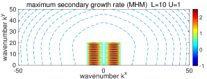
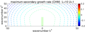
(a)

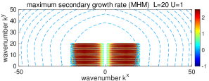
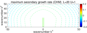
(b)

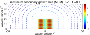
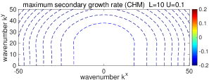
(c)

Figure 1: Maximum growth rate at each spectral mode from the secondary stability analysis according to the drift wave base flow $\mathbf{p}=\left(0,1\right)$. Solid lines are for positive growth rates and dashed lines are for negative damping rates. Results for the MHM model (left) and for the CHM model (right) in same parameter domains are compared. Different characteristic scales for $\left(L,U\right)$ are compared. The other parameters used are $\kappa=0.5,D=5\times 10^{-4}$. Notice the large amplitudes in the MHM model and small values in the CHM model from the colorbars.

For a more detailed comparison about the model instability changing with characteristic scales, the maximum growth with different parameter values $L$ and $U$ are compared. As shown in the three rows of Figure 1, larger characteristic scale $L=20$ in the drift waves induces larger number of unstable zonal modes in higher wavenumbers and stronger growth rate. In comparison, the CHM model results have little change with only negative eigenvalues for stability. Figure 2 shows the maximum growth rate $\mu$ depending on different model scales $U$ and $L$ from secondary stability analysis along the zonal modes $k^{y}=0$. More clearly, the MHM model gets unstable zonal modes from the drift wave state, while the CHM model has no instability at all along the zonal direction. For the MHM model, the largest growth gets saturated at large values of flow amplitude $U$; and with decreasing amplitudes of $U$, the growth rate drops slowly and will finally vanish at the extremely small value $U<0.01$ where the effective dissipation $D^{\prime}=\frac{D}{UL}$ becomes strong. On the other hand for the CHM model, at most weak instability is induced for large value of $U$ around the largest scales. The positive growth rate quickly vanishes as the flow strength $U$ decreases in value. This is also reflected in the contour plots in Figure 1.

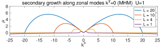
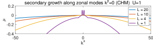
(a)

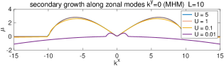
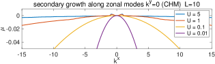
(b)

Figure 2: Maximum growth rate from secondary stability analysis along the zonal mode direction with $k^{y}=0$ for the MHM and CHM models according to the drift wave base flow $\mathbf{p}=\left(0,1\right)$. Results with different characteristic length scale $L$ and background flow strength $U$ are compared.

Finally, we test the small characteristic length $L=0.01$, that is, the background drift wave state is in a very small scale. At this small length scale limit, both MHM and CHM models converge to the barotropic model with infinite (or large) deformation frequency, $q\rightarrow\nabla^{2}\varphi$ majda2003introduction ; majda2016introduction . Figure 3 shows the maximum secondary growth rate from both the MHM and CHM model results. As expected, the growth rates from the two models perform similarly at this limit where the balanced flux correction for $\tilde{\varphi}$ becomes negligible. Also the maximum growth of the perturbations takes place at the largest scales $k<1$ compared with the small characteristic scale $L$ in the background drift wave state. Besides, the maximum secondary growth stays in small amplitude with just weak instability among all the wavenumbers. This agrees with the results in lee2003stability for barotropic turbulence.

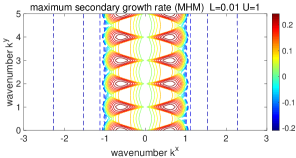
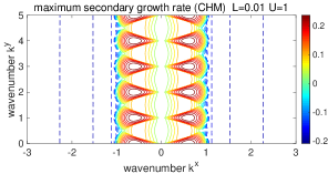
Figure 3: Real part of the secondary growth rate $\mu$ according to background base drift wave flow $\mathbf{p}=\left(0,1\right)$ with small characteristic length $L=0.01$ and $U=1$. Solid lines are for positive growth rates and dashed lines are for negative damping rates. Results for the MHM model (left) and for the CHM model (right) are compared. The other parameters used are $\kappa=0.5,D=5\times 10^{-4}$.

4.2.2 Stability about zonal flow mode $\mathbf{p}=\left(1,0\right)$

In this second test case, we consider the secondary instability due to a background zonal jet state with wave direction $\mathbf{p}=\left(1,0\right)$. In this case, a positive growth rate along the zonal modes implies further growth of the fluctuations in zonal states until higher order nonlinear interactions between modes take over. Usually, if the zonal jet amplitude keeps growing, it will finally break down due to the nonlinear interactions and cascade to the smaller scales to get dissipated. On the other hand, no instability in the zonal directions implies that the zonal jet structure is maintained stable since perturbations in zonal modes will not grow and jet structure will persist in time. This case with a zonal flow base state then characterizes the stability of the zonal structures, which can be created by the instability from drift waves through the instability analysis shown in Section 4.2.1.

In Figure 4, the maximum and minimum eigenvalues from the secondary stability analysis according to zonal jet base flow are plotted. It can be observed that there exists no positive growth rate in $\mu$ for instability at all throughout the spectral regime due to zonal flows in the MHM model. This supports the intuition described above that the induced zonal jets can be maintained stable in time in response to additional wave perturbations. In the CHM model case, the growth rate is in a similar shape but gets small positive growth near the zonal direction $k^{y}=0$. This instability in the zonal modes may imply the less stable zonal jets and the possible break down of the zonal structures due to perturbations in the CHW model. In additional, we also compare the minimum eigenvalue for the strongest damping rate in each mode from the stability analysis. The zonal modes get stronger damping at smaller scales. This again confirms the stability of the zonal jets, so that small perturbations in the zonal direction will be quickly damped down from the stabilizing effect in the background base mode.

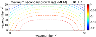
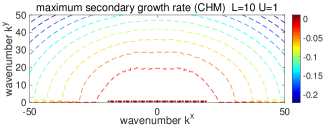
(a) maximum eigenvalue

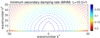
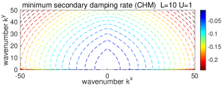
(b) minimum eigenvalue

Figure 4: Maximum growth rates and minimum damping rates for each spectral mode from largest and smallest eigenvalues in the secondary stability analysis according to zonal jet base flow $\mathbf{p}=\left(0,1\right)$. All the eigenvalues are negative in the MHM model shown in dashed lines, while the CHM model has positive growth rates near the zonal axis $k^{y}=0$. Results for the MHM model (left) and for the CHM model (right) are compared. The parameters used are $L=10,U=1$, and $\kappa=0.5,D=5\times 10^{-4}$.

Combining the conclusions of instability in the drift wave state and stability in the zonal modes, we can draw a complete picture about the energy mechanism due to the nonlinear transfer of energy in the transient state. By adopting the Hasegawa-Mima model (2) without drift wave linear instability, we start with a drift wave state that could be generated from the drift wave turbulence in the higher level Hasegawa-Wakatani model (1). The secondary instability in the drift wave base mode induces strong growth particularly along the zonal mode direction, which infers the strong transport of energy from the drift wave modes to the zonal states. After the formation of the zonal structure, the strong negative damping with no instability about the zonal jet background state shows the persistence of the zonal structure to perturbations. The zonal jets will emergence even without the help of the selective decay in dissipating small scale fluctuations described in qi2018selective .

5 Direct numerical simulations to confirm the generation of zonal jets

In this final part, we use direct numerical simulations of the MHM and CHM models (4) to confirm the theory from the secondary instability induced by the background base mode discussed in the previous section. A pseudo-spectral code with a 3/2-rule for de-aliasing the nonlinear term qi2018selective ; qi2016low is applied on the square domain with side length $L_{D}=40$ and resolution $N=256$. For the time integration, a 4th-order Runge-Kutta scheme is adopted. Small time integration step $\Delta t=1\times 10^{-4}$ is taken in all the simulations to ensure the conservation properties especially for the non-dissipative case. The same model parameter values are taken as in Section 4.2 for instability analysis.

To check the energy transfer mechanism from drift waves, the initial state of the simulations is set as a pure drift wave adding homogenous perturbations

$$\varphi_{0}=\frac{L_{D}}{s}\cos\left(\frac{2\pi s}{L_{D}}y\right)+\epsilon\sum_{\left|\mathbf{k}\right|\leq\Lambda}k^{-2}\hat{\xi}_{\mathbf{k}}e^{i\mathbf{k\cdot x}},$$ (14)

with $\hat{\xi}_{\mathbf{k}}\sim\mathcal{N}\left(0,1\right)$ sampled independently from the standard normal distribution. In practice, we add the perturbations up to wavenumber $\Lambda=5$ and the perturbation amplitude is set in a small value $\epsilon=0.01$. The parameter $s$ determines the scale of the background drift wave. We test two values with $s=2$ representing drift waves of two wavelengths and $s=10$ representing drift waves of wavenumber 10 (see the electrostatic potential $\varphi_{0}$ shown in Figure 6 for these two initial states). Besides, we consider two different situations without and with the dissipation operator $D\Delta q$ in the model.

5.1 Time evolution of energy and enstrophy in full and zonal modes

In the first numerical simulations, we introduce no dissipation effect $D=0$ in the model. Thus the conservation of total kinetic energy $E$ and potential enstrophy $W$ defined in (5) should be guaranteed. We run the model in this way so that the selective decay effect qi2018selective will be excluded. Therefore if zonal structures are generated in the final steady state from the simple drift wave initial state (14), the mechanism can only be the secondary interactions between the initial background state $\varphi_{0}$ and the perturbed small modes.

We need to confirm in the first place that the numerical dissipations have little effect in changing the model energy and enstrophy and offer no contribution in the final state of the model. For checking the conservation in the model simulations, the first two rows of Figure 5 plot the time-series of the total energy $E$ and enstrophy $W$ from the direct model simulations. In both the MHM and CHM model results, the total energy and enstrophy are conserved in time with at most small decrease in the enstrophy due to the numerical dissipation strongest at the smallest scales. Further we plot the energy and enstrophy only contained in the zonal state $\overline{\varphi}$ and $\overline{q}$. The ratio of energy in zonal velocity $v^{2}/\left(u^{2}+v^{2}\right)$ is used to characterize the flow structure, which reaches 1 when the purely zonal flow is reached. In the MHM model, the zonal energy and enstrophy start near zero in the initial time due to the initial setup, then the secondary instability takes over and the zonal energy and enstrophy jump to a large non-zero value through the nonlinear interaction. This infers the strong instability from drift wave modes and stability in the zonal jet states. In contrast, the zonal energy and enstrophy in the CHM stay in small values near zero throughout the time evolution. Then no zonal state is excited in the CHM model from the nonlinear effect.

In the last two rows of Figure 5, the time-series of energy and enstrophy as well as the zonal energy ratio with a small dissipation $D=5\times 10^{-4}$ are plotted. In comparison with the non-dissipative case before, the energy and enstrophy are no longer conserved. Especially, the enstrophy decays in a faster rate than the energy, implying that the dissipation is stronger on damping the smaller scale modes. Still, the MHM case induces strong zonal structures as the system approaches the final state. The CHM model still lacks the skill in generating zonal jets, while a pure single drift wave mode is converged consistent with the selective decay principle qi2018selective ; majda2000selective .

Most importantly, observe that in the time-series of enstrophy for the MHM model, the zonal enstrophy starts to rise at $t=2$ (marked by dashed line in the figure) while the total enstrophy begins to drop at a later time at $t=5$ (marked by dotted-dashed line). This illustrates the competition between the secondary instability and selective decay: i) during the starting time $t<2$, the initial state maintains with no linear instability; ii) between the time $2<t<5$, the secondary instability comes into effect to generate a strong zonal structure while the dissipation has no obvious effect on the smaller scale modes; iii) finally after time $t>5$, the selective decay becomes dominant and strongly dissipates the smaller scale fluctuations while maintains the created zonal jet.

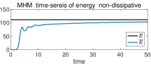
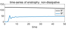
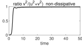
(a)

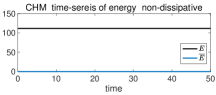
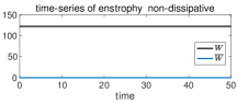
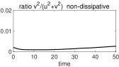
(b)

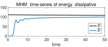
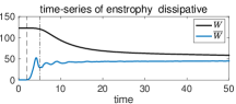
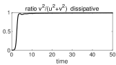
(c)

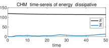
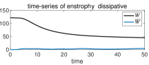
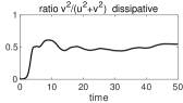
(d)

Figure 5: Time-series of the total energy $E$ and total enstrophy $W$ as well as the energy and enstrophy contained in the zonal state $\left(\overline{\varphi},\overline{q}\right)$ from the MHM and CHM model simulations. The first two rows show the results for MHM and CHM models without dissipation effect $D=0$, and the last two rows are the results for both models including weak dissipation $D=5\times 10^{-4}$. The last column plots the ratio of energy in the zonal state $v^{2}/\left(u^{2}+v^{2}\right)$.

5.2 Convergence to the final steady state without dissipation

We check the explicit flow structures from the direct numerical simulations of the MHM and CHM models. Figure 6 plots the snapshots of the electrostatic potential functions $\varphi$ from both the MHM and CHM model simulations starting from the same initial drift wave structure (14). First in the MHM model in the second column, starting from the pure drift wave state with only small isotropic perturbations (first column of Figure 6), the solutions always generate strong zonal jets in the end. This confirms the transfer of energy through the secondary instability shown in Figure 1 since no dissipation and other effect are included to generate the zonal structures. Also since there is no dissipation, the small scale non-zonal fluctuations always exist in the system on top of the zonal jets.

In comparison, the CHM model shown in the third column of Figure 6 has difficulty in generating the zonal structures. In the first case with a large scale wavenumber of two, the drift wave structure is maintained in time as the system evolves. This is consistent with the secondary stability result in the drift wave case where no positive growth rate is observed in the CHM model with a large scale base flow (see the right column of Figure 1). In the second test case with smaller scale drift wave state of wavenumber ten initially, finally the pure drift wave structure is destroyed due to the relatively stronger instability with smaller scale drift waves. Still the flow breaks into homogeneous drift wave turbulence without any zonal jet structure. This confirms the little instability in the zonal modes (only in the largest scales) in the CHM model case.

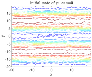
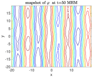
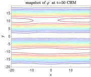
(a) initial drift wave state with wavenumber $s=2$

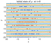
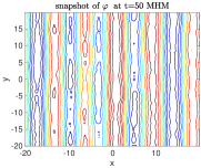
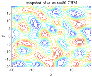
(b) initial drift wave state with wavenumber $s=10$

Figure 6: Snapshots of the electrostatic potential function $\varphi$ in the initial state (left) and the final numerical states from MHM (middle) and CHM (right) model simulations without dissipation $D=0$. Two different initial drift wave states with $s=2$ wavelengths (upper) and with $s=10$ wavelengths (lower) are compared.

5.3 Combined effects with secondary instability and selective decay

In the previous test cases, we run the models without dissipation effect. As described in qi2018selective , the damping operator usually adds stronger selective effect on the non-zonal modes and drives the flow solution to a single wavenumber state at the long time limit. Thus in this final test case, we consider the combined contributions from both the secondary instability and the selective damping. For simplicity, we introduce the simple dissipation operator, $D\Delta q$, as in (2) for both MHM and CHM models. The damping rate is kept in small value $D=5\times 10^{-4}$. In the last two rows of Figure 5, we already show the time-series of total energy and enstrophy in this case with dissipation. Both energy and enstrophy are no longer conserved in time. Still the energy/enstrophy in the zonal mean goes to the same level as the total energy/enstrophy at the long time limit in the MHM case, while the CHM only gets little energy in the zonal state.

Again, we check the final dissipated solutions from the direct numerical simulations. We plot in Figure 7 the snapshots of the electrostatic potential $\varphi$ at the final simulation time starting from the same two initial states with different drift wave scales with the inclusion of dissipation effect. Comparing with the the non-dissipative results in Figure 6, the fluctuating small-scale structures are damped down in this case while the dominant zonal structure is still maintained in the MHM model. This is the typical selective decay solution shown in Fig. 3 of qi2018selective , while here the detailed energy exchanging mechanism is discovered by the secondary instability. Observe that same number of zonal jets in the two cases is reached as in the non-dissipative results. This shows (together with the time-series of enstrophy in Figure 5) that the instability determines the final zonal structure in the first place, then the selective decay takes over to dissipate all the other non-zonal fluctuation modes to reach a clean single mode zonal state. In comparison, the CHM model converges to a drift wave selective decay state without zonal flows. With long enough time, the CHM flows will finally converge to a single drift wave mode. More detailed results about selective decay in the CHM model can be found in Fig. 1 of qi2018selective and majda2000selective .

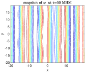
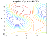
(a) initial drift wave state with wavenumber $s=2$

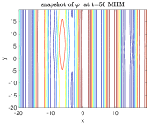
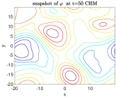
(b) initial drift wave state with wavenumber $s=10$

Figure 7: Snapshots of the electrostatic potential function $\varphi$ in the final states from MHM and CHM model simulations with dissipation $D=5\times 10^{-4}$. The same two initial drift wave states with $s=2$ and $s=10$ are compared.

5.3.1 Energy transfer mechanism in the decaying process

We offer a more detailed illustration about the energy transfer mechanism in time between different modes in the MHM model through comparing the energy spectra. In Figure 8, we plot the energy spectra in the two initial cases with and without dissipation from the MHM model simulation results. To display the transfer of energy from the non-zonal drift wave modes to the zonal modes, we compare the spectra in radially averaged modes in the first row and in zonal modes $k^{y}=0$ only in the second row. The initial spectra get a dominant second or tenth wavenumber from the initial setup (14) with small fluctuations and a high wavenumber truncation. The energy will gradually cascade to smaller scales in the transient state. A dominant zonal mode with largest energy emerges finally. With dissipation, the selective damping effect only strongly dissipates the smaller scale modes. The dominant zonal mode gets maintained at exactly the same wavenumber as the non-dissipative case and stays with large energy for all the time.

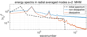
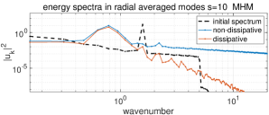
(a) energy spectra in radial averaged modes

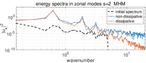
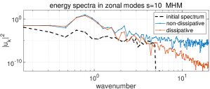
(b) energy spectra in zonal modes

Figure 8: Energy spectra in radial averaged modes (upper) and purely zonal modes (lower) from the MHM model simulations. The initial energy spectra in the two test cases are shown together with the final spectra achieved with and without dissipation effect.

Finally, to offer a complete picture about the creation of pure zonal jet structure through the combined effects of secondary instability and the selective damping, we plot the normalized energy ratio for the zonal modes $k^{y}=0$ and the non-zonal fluctuation modes at several time instant in Figure 9. In the initial state (shown in dashed black lines), all the energy is contained in the pure drift wave mode with wavenumber two ($s=2$, left) or wavenumber ten ($s=10$, right). As the starting transient state (at around time $t=3$, see also the time-series of energy and enstrophy in Figure 5), the energy in the zonal modes $k^{y}=0$ begins to grow due to the secondary instability induced by the interactions between the drift waves and zonal modes. At later time (starts from time $t=5$), the energy in the non-zonal drift wave modes begins to cascade to smaller scales and gets dissipated by the selective damping. In accordance with the time-series of energy plotted in Figure 5, the energy in the zonal modes grows rapidly between the time window $t\in\left[3,5\right]$. Then the selective damping effect takes over to drive the state to purely zonal jets. In addition, it can be observed from the energy ratios in the zonal modes that there exist several intermediate metastable saddle points which the solution visited before the convergence to the final stable single selective decay zonal mode (see qi2018selective for a complete description of the selective decay).

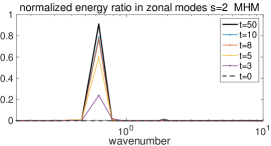
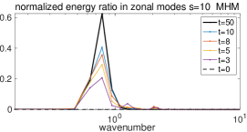
(a)

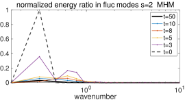
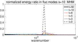
(b)

Figure 9: Selective decay of the fluctuation modes to pure zonal modes in the MHM model from the energy ratios captured at several representative time instant during the model evolution. The total energy is normalized to one to emphasize the portion of energy in each mode.

6 Concluding discussion

In this paper, we perform secondary instability analysis about a background base state to explain the zonal jet creation mechanism generally observed in plasma edge turbulence. The one-state modified Hasegawa-Mima model without internal drift wave instability is adopted to identify the central drift wave – zonal flow nonlinear interactions, and the results are compared with the Charney-Hasegawa-Mima model. Together with the selective decay principle developed previously in qi2018selective , a complete picture for the generation and persistence of a dominate zonal jet structure can be drawn. Starting from a drift wave base state created from the first linear drift wave instability, secondary instability due to nonlinear coupling with the fluctuation modes gradually takes over and transfers the energy in the non-zonal drift wave states to the zonal states. The induced zonal mode as a background state is further stabilized from the negative secondary damping effect from interacting with the perturbations. The small scale fluctuations from the initial state are maintained if no dissipation exists in the system, otherwise the selective decay effect will strongly dissipate the smaller scale modes while it does not alter the dominant zonal structure created from the instability. Direct numerical simulations of the MHM model display the creation of zonal flows from a pure non-zonal drift wave state with only small perturbation and without the effect of selective decay. When dissipation is also added, secondary instability is effective before the selective decay to generate the same number of zonal jets, and the selective decay effect finally drives the state to a clean single mode zonal jet structure. In contrast, the CHM model cannot create zonal flows automatically and has no instability along the zonal model direction.

Here we focus on the main energy mechanism for the creation of zonal structures, thus a single mode base mode is always used throughout the paper in illustrating the central role of secondary instability. As an immediate generalization, the secondary instability with combined effects with multiple background modes can be investigated. The multiple background base modes should show stronger dominant exponential growth along the zonal direction since different base modes enforce the instability in the zonal modes together and have cancellation effect in the non-zonal directions. As a further generalization, it is useful to consider the instability in the two-state Hasegawa-Wakatani models. There we need to consider the first linear instability in the base mode together with the secondary instability on top of the stable/unstable base modes. Especially, it is interesting to investigate the regime with large values of adiabatic resistivity $\alpha$, where the model is on its way to approach the MHM model discussed here.

- (1) Dewar, R.L., Abdullatif, R.F.: Zonal flow generation by modulational instability. In: Frontiers in Turbulence and Coherent Structures, pp. 415–430. World Scientific (2007)
- (2) Diamond, P.H., Itoh, S., Itoh, K., Hahm, T.: Zonal flows in plasma—a review. Plasma Physics and Controlled Fusion 47(5), R35 (2005)
- (3) Fujisawa, A.: A review of zonal flow experiments. Nuclear Fusion 49(1), 013001 (2009). URL http://stacks.iop.org/0029-5515/49/i=1/a=013001
- (4) Hasegawa, A., Mima, K.: Pseudo-three-dimensional turbulence in magnetized nonuniform plasma. The Physics of Fluids 21(1), 87–92 (1978)
- (5) Hasegawa, A., Wakatani, M.: Plasma edge turbulence. Physical Review Letters 50(9), 682 (1983)
- (6) Horton, W.: Drift waves and transport. Rev. Mod. Phys. 71, 735–778 (1999). DOI 10.1103/RevModPhys.71.735. URL https://link.aps.org/doi/10.1103/RevModPhys.71.735
- (7) Lee, Y., Smith, L.M.: Stability of rossby waves in the -plane approximation. Physica D: Nonlinear Phenomena 179(1-2), 53–91 (2003)
- (8) Lin, Z., Hahm, T.S., Lee, W.W., Tang, W.M., White, R.B.: Turbulent transport reduction by zonal flows: Massively parallel simulations. Science 281(5384), 1835–1837 (1998). DOI 10.1126/science.281.5384.1835. URL http://science.sciencemag.org/content/281/5384/1835
- (9) Majda, A.: Introduction to PDEs and Waves for the Atmosphere and Ocean, vol. 9. American Mathematical Soc. (2003)
- (10) Majda, A.J.: Introduction to turbulent dynamical systems in complex systems. Springer (2016)
- (11) Majda, A.J., Qi, D.: Strategies for reduced-order models for predicting the statistical responses and uncertainty quantification in complex turbulent dynamical systems. SIAM Review 60(3), 491–549 (2018)
- (12) Majda, A.J., Qi, D., Cerfon, A.J.: A flux-balanced fluid model for collisional plasma edge turbulence: Model derivation and basic physical features. Physics of Plasmas 25(10), 102307 (2018). DOI 10.1063/1.5049389. URL https://doi.org/10.1063/1.5049389
- (13) Majda, A.J., Shim, S.Y., Wang, X.: Selective decay for geophysical flows. Methods and applications of analysis 7(3), 511–554 (2000)
- (14) Manfredi, G., Roach, C., Dendy, R.: Zonal flow and streamer generation in drift turbulence. Plasma physics and controlled fusion 43(6), 825 (2001)
- (15) Manz, P., Ramisch, M., Stroth, U.: Physical mechanism behind zonal-flow generation in drift-wave turbulence. Phys. Rev. Lett. 103, 165004 (2009). DOI 10.1103/PhysRevLett.103.165004. URL https://link.aps.org/doi/10.1103/PhysRevLett.103.165004
- (16) Meshalkin, L.: Investigation of the stability of a stationary solution of a system of equations for the plane movement of an incompressible viscous liquid. J. Appl. Math. Mech. 25, 1700–1705 (1962)
- (17) Numata, R., Ball, R., Dewar, R.L.: Bifurcation in electrostatic resistive drift wave turbulence. Physics of Plasmas 14(10), 102312 (2007)
- (18) Pedlosky, J.: Geophysical fluid dynamics. Springer Science & Business Media (2013)
- (19) Pushkarev, A.V., Bos, W.J.T., Nazarenko, S.V.: Zonal flow generation and its feedback on turbulence production in drift wave turbulence. Physics of Plasmas 20(4), 042304 (2013). DOI 10.1063/1.4802187. URL https://doi.org/10.1063/1.4802187
- (20) Qi, D., Majda, A.J.: Low-dimensional reduced-order models for statistical response and uncertainty quantification: Two-layer baroclinic turbulence. Journal of the Atmospheric Sciences 73(12), 4609–4639 (2016)
- (21) Qi, D., Majda, A.J.: Transient metastability and selective decay for the coherent zonal structures in plasma edge turbulence. submitted to Journal of Nonlinear Science (2018)
- (22) Qi, D., Majda, A.J., Cerfon, A.J.: A Flux-Balanced Fluid Model for Collisional Plasma Edge Turbulence: Numerical Simulations with Different Aspect Ratios. submitted to Physics of Plasmas arXiv:1812.00131 (2018)
- (23) Rhines, P.B.: Waves and turbulence on a beta-plane. Journal of Fluid Mechanics 69(3), 417–443 (1975)
- (24) Smolyakov, A., Diamond, P., Malkov, M.: Coherent structure phenomena in drift wave–zonal flow turbulence. Physical review letters 84(3), 491 (2000)
- (25) Xanthopoulos, P., Mischchenko, A., Helander, P., Sugama, H., Watanabe, T.H.: Zonal flow dynamics and control of turbulent transport in stellarators. Phys. Rev. Lett. 107, 245002 (2011). DOI 10.1103/PhysRevLett.107.245002. URL https://link.aps.org/doi/10.1103/PhysRevLett.107.245002