Operational relevance of resource theories of quantum measurements
Abstract
For any resource theory it is essential to identify tasks for which resource objects offer advantage over free objects. We show that this identification can always be accomplished for resource theories of quantum measurements in which free objects form a convex subset of measurements on a given Hilbert space. To this aim we prove that every resourceful measurement offers advantage for some quantum state discrimination task. Moreover, we give an operational interpretation of robustness, which quantifies the minimal amount of noise that must be added to a measurement to make it free. Specifically, we show that this geometric quantity is related to the maximal relative advantage that a resourceful measurement offers in a class of minimal-error state discrimination (MESD) problems. Finally, we apply our results to two classes of free measurements: incoherent measurements (measurements that are diagonal in the fixed basis) and separable measurements (measurements whose effects are separable operators). For both of these scenarios we find, in the asymptotic setting in which the dimension or the number of particles increase to infinity, the maximal relative advantage that resourceful measurements offer for state discrimination tasks.
1 Introduction
Resource theories [1] constitute a powerful toolbox to study physical systems in the presence of limitations resulting from experimental or operational constrains on the ability to address and manipulate physical systems. This mathematical framework is general enough to encompass both classical and quantum physics, or even more general theories [2]. In recent years it has been successfully applied to classical and quantum thermodynamics [3, 4], processing of quantum information in distributed scenarios [5, 6], contextuality [7], nonlocality [8], steering [9] and, last but not least, magic state distillation paradigm of quantum computation [10]. On the general level, all resource theories are defined by specifying free objects and free operations. Free objects form a subset of the set of all objects relevant for the physical situation in question. Likewise, free operations form a subclass of all relevant physical transformations. Typically objects that are not free are called resource objects. The specific choice of free objects and free operations depends on the physical context. For example, in entanglement theory the relevant resource theory is based on the principle of locality: set of free objects consists of separable states while free operations are all local operations assisted by classical communication (LOCC).
For any resource theory it is desirable to give operational interpretation of resource objects i.e to identify a task for which a given resource object would prove advantageous over all free objects. The main purpose of this work is to provide such interpretations for resource theories in which a set of free objects consists of convex subset of the set of quantum measurements (POVMs) on a relevant Hilbert space. We realize this goal by showing, that in this setting for every resourceful measurement there an instance of minimal-error quantum state discrimination game for which gives greater success probability then all free measurements. Quantum state discrimination [11, 12] is a popular quantum information subroutine that finds applications in different areas of quantum information science including quantum communication [13], quantum metrology [14], nonlocality [15] or quantum computation [16]. We push our operational interpretation further by proving the quantitative relation between the relative advantage of resourceful measurement for state discrimination and the geometric measure of resourcefulness called robustness [17, 18], which quantifies the minimal amount of noise that has to be added to a POVM to make it free. Previously, the measure robustness was introduced [19] to mathematically quantify entanglement. Leter, it was employed in the general resource- theoretic framework [20, 21, 1].
We apply our general results to two classes of free measurements: incoherent measurement and separable measurements. Incoherent measurements are POVM analogues of incoherent states [22, 23, 24] and can be understood as measurements originating from a single projective measurement (in the fixed basis) followed by arbitrary classical post-processing. Separable measurements [25, 26, 27, 28], on the other hand, are POVMs on composite quantum systems whose effects are separable operators. This class contains the set of LOCC measurements [29, 30] i.e. measurements that can be implemented via local measurements and LOCC operations. For both incoherent and separable measurements we focus on the asymptotic setting in which the dimension of the system or the number of particles involved go to infinity. In this regime we identify, for both classes of measurements, the maximal relative advantage that resourceful measurements can offer for quantum state discrimination tasks.
Traditionally, operational interpretations of quantum resources were developed case-by-case for different resource theories [31, 32, 33, 34, 35, 36]. A recent paper [18] gave an unified treatment of this problem for all quantum resource theories in which the set of free objects is convex subset of the set of quantum states. Specifically, the authors of this work showed that in this context all resource states offer advantage for some sub-channel discrimination problem (this result was previously obtained for resource theories of entanglement [37], coherence [38], steering [39] and asymmetry [40]). Our results are complementary to [18], as they give the operational interpretation of all convex resource theories of quantum measurements. Moreover, our work greatly generalizes some of the results of [17], where the analogous analysis was presented for the case where free measurements consisted of maximally uninformative measurements i.e. measurements that do not recover any information about the measured quantum states.
So far, research in quantum resource theories focussed mainly on quantum states while quantum measurements, despite their importance, did not receive much attention. Previously, resource-theoretic perspective was applied in the context of measurement incompatibility [41, 42], measurement simulability via projective measurements [43, 44], and simulability in the more general scenarios [42, 45]. We believe that our results, especially previously unexplored quantitative relation between state discrimination and robustness, provide new quantitative tools to study the restricted classes of POVMs and, more generally, quantum resource theories concentrated around quantum measurements.
2 Notation and main concepts
Throughout the paper we will be interested in POVMs on finite dimensional Hilbert space . Such generalized measurements (POVMs) can be understood as tuples of non-negative operators on satisfying , where is the number of outcomes and is the identity on . The operators are called the effects of POVM . According to Born’s rule, when a POVM is measured on a quantum state the probability of obtaining the outcome is given by . We denote the set of POVMs on with outcomes by . This set has a natural convex structure [46]: given two POVMs , their convex combination is the POVM with -th effect given by . The operation of taking convex combinations of measurements can be operationally realized as performing POVMs and with certain probabilities and then combining the outcomes.
Our operational interpretation of resourcefullness of quantum measurements will be based on the task of minimal-error state discrimination [11, 12]. The purpose of this task is to optimally distinguish quantum states states generated by the ensemble , where is a probability distribution and is a collection of quantum states. The success probability of identifying the states generated by via a measurement is given by
| (1) |
One is often interested in choosing the measurement , such that is maximized. However, if only a restricted class of measurements is allowed, the maximum may not be achieved.
3 Convex resource theories of measurements and measurement robustness
We now give a minimal formulation of a resource theory of measurements, under the assumption of convexity. In our treatment we will focus on a set of quantum measurements and a class of free operations 111Of course, the full treatment of resource theory of measurements requires to take into account more complicated aspects such as composability. We plan to address such questions in the future work. . We first assume (i) that the set of free measurements is a convex and closed subset of -outcome measurements on i.e , for some suitable Hilbert space . Second, we assume that the class of free operations consists of mappings that (ii) preserve the set of free measurements i.e. for all we have and (iii) are convex-linear i.e. for all measurements .
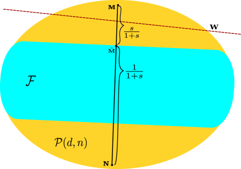
Justification of assumptions: The convexity of can be justified by the fact that, as argued before, convex combination of measurements can be realised by a purely classical process. The compactness of is a technical assumption that allows us to formally state our results. However, in basically any physically interesting case the class of free measurements can be viewed as a set of convex combinations (convex hull) of a compact set of "primitive" measurements , and hence is naturally compact. Finally, convex linearity of free operations follows from linearity of quantum mechanics while preservation of the by free operation is also natural - operations that are considered free should not be able to create resourceful measurement. In particular, in many cases the set contains (a) classical post-processing i.e. operation of the form , where , for some stochastic matrix , and (b) unitary symmetries of the set .
For every set of free measurements it is possible to introduce a geometric measure quantifying the minimum amount of noise which has to be added to a given POVM to make it free. In analogy to previous works [19, 18, 17] we will call this quantifier robustness and denote it by . It is formally defined in the following way (See Fig. 1):
| (2) |
The robustness enjoys a number of natural properties as stated by the following proposition.
Proposition 1 (Properties of robustness).
Let be a closed convex set of free measurements. The robustness satisfies the following properties: (i) Faithfulness: and iff , (ii) Convexity: , (iii) Monotonicity under free operations: for all free operations .
The proof of the above follows directly form the definitions of the concepts involved and we defer it to the Appendix.
4 Main results
In this part we give our main results concerning the operational interpretation of resourceful measurements for a class of quantum state discrimination tasks.
Theorem 1 (Minimal-error state discrimination
can certify resource character of measurements).
For any resourceful POVM , there exist an ensemble such that
| (3) |
Proof.
We begin the proof by noting that is a convex subset of where is a - dimensional Hilbert space and is the set of hermitian operator from to itself. The space can be regarded as dimensional real vector space with the inner product defined by , where . We have assumed that is a compact set and hence, due to hyperplane separation theorem (see Fig. 1), for any , there exists a tuple of Hermitian operators such that while for all we have . We now define , where is the smallest eigenvalue of operators . We note that for every the operator is positive-semi-definite and moreover . Using this we construct the ensemble , for which the inequality (3) holds. ∎
The above result shows the qualitative advantage of resourceful measurements for a class of state-discrimination tasks. In what follows we show a natural way to quantify this advantage. In Theorem 2 below we show that under the same assumptions as above, the robustness is related to the maximal relative advantage that a resourceful measurement offers for MESD. To prove this result we will use the following technical Lemma that can be regarded as dual characterisation of measurement robustness. Its proof relies on duality of semi-infinite convex optimization programs [47] and we present it in the Appendix.
Lemma 1.
Let and be a compact convex set of free measurements. Then, the generalized robustness can be expressed as the following optimisation problem.
| maximize | (4) | |||||
| subject to | ||||||
We are now ready to state and prove our main result.
Theorem 2 (Operational interpretation of robustness in terms of quantum state discrimination).
For any class of free measurements and any POVM the generalized robustness can be expressed as
| (5) |
where the outer optimisation is over element ensembles of quantum states.
Proof.
We begin by showing that LHS(5) RHS(5). From the definition of generalized robustness from (2) it follows that for each effect of POVM it holds that , where are the effects of POVM and are the effects of POVM . Therefore, we have for every and therefore
| (6) | |||
where the second inequality follows from .
To show LHS(5) RHS(5), we use the dual characterization of the generalized robustness from Lemma 1. Let be the optimal tuple for which (4) is maximized. We now define
| (7) |
Simple algebraic manipulations give . On the other hand from (4) it follows that we have . Using these two properties we obtain
| (8) |
Importantly, Theorems 1 and 2 are valid for all convex and compact sets of free measurements . In particular, we can directly apply them to the measurements that are simulable by projective measurements [43, 44] or -outcome measurements [42, 45]. In what follows, we will consider application of our results to two other classes of free measurements: incoherent measurements and separable measurements. We will focus on obtaining the maximal relative advantage for MESD that can be obtained in these scenarios by resourceful measurements.
4.1 Incoherent measurements
Quantum coherence or superposition is one of the salient nonclassical aspects of quantum theory. Recently, this feature of quantum theory was investigated thoroughly form the resource-theoretic perspective [23, 24]. Moreover, quantum coherence has been identified as resource for a number of quantum information processing tasks like quantum channel discrimination [37], designing quantum algorithms [48], quantum metrology [14] and quantum thermodynamics [3]. Finally, there is a plethora of works on quantification of quantum coherence of quantum states [23, 49] and operations [50, 51] and on giving operational interpretation to some quantifiers [35, 36].
Here we propose to introduce a concept of coherence to the realm of POVMs. Specifically, we define the class of incoherent measurements consisting of -outcome measurements S on , whose effects are diagonal in a particular orthogonal basis . In what follows, for the sake of simplicity, we assume . Incoherent measurements constitute a POVM analogues of the set of incoherent states. More formally, the effects of incoherent measurements S can be expressed as , where . In is now easy to see that incoherent measurements can always be obtained via classical post-processing of projective measurements in the standard basis.
One way to quantify the coherence present in a POVM is the robustness with respect to the set of incoherent measurements. Importantly, satisfies a number of natural properties stated in Lemma 1. Here, the class of free operations can be chosen to contain all diagonal unitaries and classical post-processing 222In fact all quantum channels such that is an incoherent channel also preserve .. By applying Theorem 2 directly to this setting we get that robustness , can be identified as the maximal relative advantage of for a suitable state discrimination problem. In the following we will take the complemenary approach based on semi-definite programming [52]. From the definition of incoherent measurements it follows that can be casted as the following semi-definite program (SDP)
| minimize | (9) | |||||
| s.t | ||||||
Taking the dual problem we get the following auxiliary result whose proof we defer to the Appendix.
Lemma 2 (Dual characterization of robustness w.r.t. incoherent measurement).
Robustness of a POVM w.r.t set of incoherent measurement , i.e, can be expressed as the solution of optimization problem given by
| maximize | (10) | |||||
| subject to | ||||||
From the above we get a physical characterization of ensembles of states that suffice to capture the maximal advantage of coherent measurements over the incoherent ones.
Proposition 2 (Alternative characterisation of robustness for incoherent measurements).
Let . We have the following equality
| (11) |
where the outer optimisation is over ensembles consisting of states that cannot be classically distinguished [53] (that is, for all and for all we have ). Due to this property of for all incoherent measurements we have .
Proof.
The above operational characterisation of allows us to identify measurements with the greatest possible robustness (hence relative advantage for MESD) in a given dimension .
Proposition 3 (Maximal advantage of coherent measurements over incoherent measurements).
The following equality holds
| (12) |
Moreover, when the measurement attains the maximal value of if and only if its effects are proportional to maximally coherent states i.e pure states of the form .
Proof.
From Lemma 2 it follows that , where cannot be classically distinguished. Since for any we have we obtain . Moreover, if this bound can be easily saturated for projective measurements in the Fourier basis =with ensemble .
For , we will use (10) to get the missing upper bound. We first note that since operators are upper bounded by we have . Therefore , from (10) we can conclude that , hence .
Combining this with the previous case we conclude .
Just like in the case we will proof the saturation of this bound using Fourier transform of the original basis . To prove the equality for the case , we choose an ensemble uniformly distributed over first orthonormal states from ensemble , i.e, and an outcome POVM . For this particular case, again RHS of (11) reduce to . Combining these two cases we obtain .
Now we will show that for any POVM for which (11) holds, have the effects directly proportional to where . This follows from the simple observation that for , maximization of (10) , requires that , where . Moreover, to satisfy the constraint of (10), has to be one dimensional. This implies only feasible solution will be
| (13) |
where is rank one projector with trace 1. Then to be a valid POVM,
| (14) |
Combining (14) and (10) we obtain for every . This leads to the conclusion that the POVM with outcomes and satisfying must have effects proportional to where . ∎
4.2 Separable measurements
We now turn our attention to the measurements that can be performed on a composite quantum systems. In what follows we will study the maximal advantage that entangled measurements can offer for MESD over so-called separable measurements on multiparticle quantum systems. Separable measurements contain the set of LOCC measurements and are relatively easy to characterize. For this reason the maximal advantage with respect to separable measurements is in general smaller then the advantage with respect to LOCC measurements.
Consider a biparticle quantum system . We define a POVM as separable if all its effects are separable operators i.e. where and are positive operators on and respectively. The above definition can be easily extended to system of multiple qubits . We denote the set of biparticle separable measurements by and separable multiqubit measurements by . Recall that we made the dependence on number of outcomes implicit. In what follows we will assume that is fixed and equals at least the dimension of the relevant Hilbert space ( and respectively). It easily follows that and are convex compact subsets of for suitable Hilbert spaces. The following Lemma gives the comprehensive answer to the question about the maximal advantage for MESD that entangled measurements can offer over separable measurements in both bipartite and multiparty scenario.
Proposition 4 (Maximal advantage of entangled meaurements over separable measurements).
Let and denote the dimensions of local spaces in the biparticle Hilbert space . Then, the following inequalities hold
| (15) |
where the maximization is over all measurements on .
Moreover, the maximal robustness of entangled qubit measurement increases exponentially with the size of the system. Specifically, for sufficiently large we have
| (16) |
where the maximization is over all measurements on and .
Sketch of the proof.
The upper bounds in (15) and (16) follow from application of explicit simulation strategy based on (global) depolarizing map . This map, transforms effects of a measurement as follows: . It is easy to check that the resulting operators still form a POVM on a total space. Because this map preserves traces of the effects we can write , where is a quantum state. To get an upper bound on the robustness of it that suffices to find lower bond on defined as the number for which all states constructed from the effects of are separable. To find the upper bound we can directly use the results from entanglement theory. Concretely, the problem of how much "white noise" can be added to a quantum state before it becomes separable quantum states has been studied before. Specifically the maximal value of "random robustness" (minimal such that is separable) equals in the biparticle scenario [19] and can be upper bounded by for the multipartice case [54]. To obtain the lower bounds we use characterization of the robustness MESD given in Eq.(5) by showing advantage of entangled measurements over separable ones for particular uniform ensambles of quantum states. for biparticle case we consider exnamble consisting of orthogonal maximally states [29], while for multiparticle case we consider ensemble consisting of iid random quantum states taken from the Haar measure on [55] (see Appendix for details). ∎
Remark.
The above results complement existing results [56, 29, 57] on the relative power of LOCC separable, and global state discrimination. Our focus was on the advantage in discrimination of arbitrary ensembles of quantum states while previously the emphasis was put mostly on ensembles consisting of two states (for example in the context of quantum data hiding).
5 Open problems
We finish with giving possible directions of further study. First, it is tempting to ask if non-free character of measurements can be certified in a device-independent manner in prepare-and measure scenarios [58, 59]. Second interesting problem concerns finding the maximal that resourceful POVMs advantage for state discrimination problems for other important classes of measurements such as LOCC measurements [29, 30] or projective-simulable measurements [43, 44]. The potential lack of the increasing separation (as ) between projective and general POVMs will likely have strong consequences for quantum information processing and Bell nonlocality. Finally, it is natural to ask if analogous operational interpretations hold also for other classes of quantum objects such as quantum channels or quantum instruments.
Note added—- Upon the completion of this work we became aware of two works [60, 61] that independently obtained results overlapping with Theorem 2 presented here. Moreover, similar methods were used in the context of measurement incompatibility [62, 63].
References
- Chitambar and Gour [2018] E. Chitambar and G. Gour, arXiv:1806.06107 (2018).
- Coecke et al. [2016] B. Coecke, T. Fritz, and R. W. Spekkens, Information and Computation 250, 59 (2016).
- Brandão et al. [2013] F. G. S. L. Brandão, M. Horodecki, J. Oppenheim, J. M. Renes, and R. W. Spekkens, Phys. Rev. Lett. 111, 250404 (2013).
- Goold et al. [2016] J. Goold, M. Huber, A. Riera, L. del Rio, and P. Skrzypczyk, Journal of Physics A: Mathematical and Theoretical 49, 143001 (2016).
- Vedral et al. [1997] V. Vedral, M. B. Plenio, M. A. Rippin, and P. L. Knight, Phys. Rev. Lett. 78, 2275 (1997).
- Horodecki et al. [2009] R. Horodecki, P. Horodecki, M. Horodecki, and K. Horodecki, Rev. Mod. Phys. 81, 865 (2009).
- Grudka et al. [2014] A. Grudka, K. Horodecki, M. Horodecki, P. Horodecki, R. Horodecki, P. Joshi, W. Kłobus, and A. Wójcik, Phys. Rev. Lett. 112, 120401 (2014).
- Barrett [2007] J. Barrett, Phys. Rev. A 75, 032304 (2007).
- Gallego and Aolita [2015] R. Gallego and L. Aolita, Phys. Rev. X 5, 041008 (2015).
- Veitch et al. [2012] V. Veitch, C. Ferrie, D. Gross, and J. Emerson, New Journal of Physics 14, 113011 (2012).
- Barnett and Croke [2009] S. M. Barnett and S. Croke, Adv. Opt. Photon. 1, 238 (2009).
- Bae and Kwek [2015] J. Bae and L.-C. Kwek, J. Phys. A: Math. Gen. 48, 083001 (2015).
- Brunner et al. [2013] N. Brunner, M. Navascués, and T. Vértesi, Phys. Rev. Lett. 110, 150501 (2013).
- Marvian and Spekkens [2016] I. Marvian and R. W. Spekkens, Phys. Rev. A 94, 052324 (2016).
- Bae et al. [2011] J. Bae, W.-Y. Hwang, and Y.-D. Han, Phys. Rev. Lett. 107, 170403 (2011).
- Lomont [2005] C. Lomont, arxiv:0411037 (2005).
- Skrzypczyk and Linden [2019] P. Skrzypczyk and N. Linden, Phys. Rev. Lett. 122, 140403 (2019).
- Takagi et al. [2018] R. Takagi, B. Regula, K. Bu, Z.-W. Liu, and G. Adesso, Phys. Rev. Lett. 122, 140402 (2019).
- Vidal and Tarrach [1999] G. Vidal and R. Tarrach, Phys. Rev. A 59, 141 (1999).
- Brandão and Gour [2015] F. G. S. L. Brandão and G. Gour, Phys. Rev. Lett. 115, 070503 (2015).
- Regula [2017] B. Regula, Journal of Physics A: Mathematical and Theoretical 51, 045303 (2017).
- Aberg [2006] J. Aberg, arXiv:quant-ph/0612146 (2006).
- Baumgratz et al. [2014] T. Baumgratz, M. Cramer, and M. B. Plenio, Phys. Rev. Lett. 113, 140401 (2014).
- Streltsov et al. [2017] A. Streltsov, G. Adesso, and M. B. Plenio, Rev. Mod. Phys. 89, 041003 (2017).
- Bandyopadhyay and Nathanson [2013] S. Bandyopadhyay and M. Nathanson, Phys. Rev. A 88, 052313 (2013).
- Watrous [2018] J. Watrous, The Theory of Quantum Information (Cambridge University Press, 2018).
- Bagan et al. [2005] E. Bagan, M. A. Ballester, R. Muñoz Tapia, and O. Romero-Isart, Phys. Rev. Lett. 95, 110504 (2005).
- Kargin [2004] V. Kargin, The Annals of Statistics 33, 959 (2004).
- Nathanson [2005] M. Nathanson, J. Math. Phys. 46, 141 (2005).
- Chitambar et al. [2014] E. Chitambar, D. Leung, L. Mančinska, M. Ozols, and A. Winter, Communications in Mathematical Physics 328, 303 (2014).
- D’Ariano et al. [2001] G. M. D’Ariano, P. Lo Presti, and M. G. A. Paris, Phys. Rev. Lett. 87, 270404 (2001).
- Horodecki and Oppenheim [2013] M. Horodecki and J. Oppenheim, Nat. Commun. 4 (2013), 10.1038/ncomms3059.
- Spekkens et al. [2009] R. W. Spekkens, D. H. Buzacott, A. J. Keehn, B. Toner, and G. J. Pryde, Phys. Rev. Lett. 102, 010401 (2009).
- Cavalcanti et al. [2017] D. Cavalcanti, P. Skrzypczyk, and I. Šupić, Phys. Rev. Lett. 119, 110501 (2017).
- Winter and Yang [2016] A. Winter and D. Yang, Phys. Rev. Lett. 116, 120404 (2016).
- Biswas et al. [2017] T. Biswas, M. G. Diaz, and A. Winter, Proc. R. Soc. A 473 (2017), 10.1098/rspa.2017.0170.
- Piani et al. [2016a] M. Piani, M. Cianciaruso, T. R. Bromley, C. Napoli, N. Johnston, and G. Adesso, Phys. Rev. A 93, 042107 (2016a).
- Napoli et al. [2016] C. Napoli, T. R. Bromley, M. Cianciaruso, M. Piani, N. Johnston, and G. Adesso, Phys. Rev. Lett. 116, 150502 (2016).
- Piani and Watrous [2015] M. Piani and J. Watrous, Phys. Rev. Lett. 114, 060404 (2015).
- Piani et al. [2016b] M. Piani, M. Cianciaruso, T. R. Bromley, C. Napoli, N. Johnston, and G. Adesso, Phys. Rev. A 93, 042107 (2016b).
- Heinosaari et al. [2015] T. Heinosaari, J. Kiukas, and D. Reitzner, Phys. Rev. A 92, 022115 (2015).
- Guerini et al. [2017] L. Guerini, J. Bavaresco, M. Terra Cunha, and A. Acín, J. Math. Phys. 58, 092102 (2017).
- Oszmaniec et al. [2017] M. Oszmaniec, L. Guerini, P. Wittek, and A. Acín, Phys. Rev. Lett. 119, 190501 (2017).
- Oszmaniec et al. [2018] M. Oszmaniec, F. B. Maciejewski, and Z. Puchała, arXiv:1807.08449 (2018).
- Kleinmann and Cabello [2016] M. Kleinmann and A. Cabello, Phys. Rev. Lett. 117, 150401 (2016).
- D’Ariano et al. [2005] G. M. D’Ariano, P. L. Presti, and P. Perinotti, J. Phys. A: Math. Gen. 38, 5979 (2005).
- Brandao [2005] F. G. Brandao, Phys. Rev. A 72, 022310 (2005).
- Hillery [2016] M. Hillery, Phys. Rev. A 93, 012111 (2016).
- Bischof et al. [2018] F. Bischof, H. Kampermann, and D. Bruss, arXiv:1812.00018 (2018).
- Theurer et al. [2018] T. Theurer, D. Egloff, L. Zhang, and M. B. Plenio., arXiv:1806.07332 (2018).
- Bera [2018] M. Bera, arXiv:1809.02578 (2018).
- Vandenberghe and Boyd [1996] L. Vandenberghe and S. Boyd, SIAM Review 38, 49 (1996).
- Korzekwa et al. [2018] K. Korzekwa, S. Czachorski, Z. Puchała, and K. Zyczkowski, arXiv:1812.09083 (2018).
- Gurvits and Barnum [2003] L. Gurvits and H. Barnum, Phys. Rev. A 68, 042312 (2003).
- Montanaro [2007] A. Montanaro, Commun Math Phys 273, 619 (2007).
- Hayden et al. [2004] P. Hayden, D. Leung, P. W. Shor, and A. Winter, Communications in Mathematical Physics 250, 371 (2004).
- Matthews et al. [2009] W. Matthews, S. Wehner, and A. Winter, Communications in Mathematical Physics 291, 813 (2009).
- Tavakoli et al. [2018] A. Tavakoli, M. Smania, T. Vértesi, D. Rosset, and N. Brunner, arXiv:1811.12712 (2018).
- Mironowicz and Pawłowski [2018] P. Mironowicz and M. Pawłowski, arXiv:1811.12872 (2018).
- Uola et al. [2018] R. Uola, T. Kraft, J. Shang, X.-D. Yu, and O. Guhne, Phys. Rev. Lett. 122, 130404 (2019).
- R. and Regula [2019] R. Takagi. and B. Regula, arXiv:1901.08127 (2019).
- Carmeli et al. [2018] C. Carmeli, T. Heinosaari, and A. Toigo, Phys. Rev. Lett. 122, 13040 (2019).
- Skrzypczyk et al. [2019] P. Skrzypczyk, I. Šupić, and D. Cavalcanti, Phys. Rev. Lett. 122, 130403 (2019).
- Cavalcanti and Skrzypczyk [2016] D. Cavalcanti and P. Skrzypczyk, Reports on Progress in Physics 80, 024001 (2016).
- Gross et al. [2009] D. Gross, S. T. Flammia, and J. Eisert, Phys. Rev. Lett. 102, 190501 (2009).
Appendix
In what follows we give proofs that were omitted in the main part of the manuscript. In Part A we give proofs concerning the general properties of the robustness and its dual formulation. In Part B we give justifications of results specific to particular scenarios of incoherent and separable measurements.
Appendix A Proofs of general results
For the convenience of the reader we first recall the definition of robustness for general convex and compact subset of free measurements
| (17) |
Proposition 1 (Properties of robustness).
Let be a compact convex set of free measurements. The robustness satisfies the following properties: (i) Faithfulness: and iff , (ii) Convexity: , (iii) Monotonicity under free operations: for all free operations .
Proof.
(i) Faithfulness. This property follows directly from the definition given in Eq.(17).
(ii) Convexity. From the definition of the robustness (17) it follows that for two POVMs there exist POVMs , such that
| (18) | |||||
| (19) |
where . We therefore get that for all
| (20) | ||||
After defining
| (21) | |||||
| (22) | |||||
| T | (23) |
we note that , while . We finally observe that
| (24) |
which directly implies .
(iii) Monotonicity under free operations. From the definition we have that for every there exist and such that
| (25) |
Applying to both sides of the above equality we obtain
| (26) |
Since, by assumption, , equation (26) directly implies . ∎
Lemma 1.
Let and be a compact convex set of free measurements. Then, the generalized robustness can be expressed as the following optimisation problem.
| maximize | (27) | |||||
| subject to | ||||||
Proof.
Our proof starategy is the following. The problem in (27) belongs to the class of semi-infinite optimisation problems [47]. We will compute its dual and argue that there is no duality gap. Finally, the dual problem will turn out to be equivalent to the original definition of robustness from (17). After simple algebraic manipulations we obtain that (27) is equivalent to
| (28) | |||
The Lagrangian corresponding to the last problem in (28) reads
| (29) |
where and are lagrange multipliers which satisfy and for almost all . To construct the dual problem to (29) we minimize over primal variables . Since the Lagrangian is affine function of , we obtain minimum equal to unless . If the condition holds then we obtain . Hence we see that the dual of the problem (27) can be written as
| minimize | (30) | |||||
| subject to | ||||||
We note that the primal problem (27) posseses a strictly feasible points (for example , for ), which follows from the assumption of the compactness of and the form of the constrains in (27). Finally, we conclude the proof by noting that iff where and . ∎
Appendix B Proofs of results that concern particular classes of free measurements
B.1 Incoherent measurements
From the definition of robustness (see Eq.(17)) and the definition of incoherent measurements we obtain that can be cast as the following SDP program
| minimize | (31) | |||||
| s.t | ||||||
.
Lemma 2 (Dual characterization of robustness w.r.t. incoherent measurement).
Robustness of a POVM w.r.t set of incoherent measurement , i.e, can be expressed as the solution of optimization problem given by
| maximize | (32) | |||||
| subject to | ||||||
Proof.
Introducing variables and we obtain an equivalent form of problem from (31)
| minimize | (33) | |||||
| subject to | ||||||
To construct the dual of the optimization problem [64, 52] given in (33), we start by writing down the Lagrangian associated with primal problem
| (34) |
where we have introduced as dual variable (Lagrange multipliers). To ensure that the Lagrangian is always smaller than the objective function whenever the constraints of the (33) are satisfied, we impose and . To ensure that the Lagrangian is independent of primal variables we have . Finally, the corresponding dual problem which sets the upper bound for primal optimization problem is given by
| maximize | (35) | |||||
| subject to | ||||||
By inspection one can conclude that strong duality holds, since satisfy the constraints in (35) and is positive-definite. Therefore, the solutions (33) and (35) are equal. ∎
B.2 Separable measurements
Proposition 4 (Maximal advantage of entangled measurements over separable measurements).
Let and denote the dimensions of local spaces in the biparticle Hilbert space . Then, the following inequalities hold
| (36) |
where the maximization is over all measurements on .
Moreover, the maximal robustness of entangled qubit measurement increases exponentially with the size of the system. Specifically, for sufficiently large we have
| (37) |
where the maximization is over all measurements on and .
Proof of lower bounds in Eq.(36) and Eq.(37).
Our strategy to prove the lower bounds is to construct ensembles for which the relative advantage
| (38) |
of some entangled measurement over the separable ones will be large. (i) Biparticle case Let . Following Nathanson [29], we consider an uniform ensemble consisting orthogonal maximally entangled states from ,
| (39) |
Since vectors are orthogonal, they can be distinguished perfectly by measurement whose effects are of the form , where are operators orthogonal to states . On the other hand there is a limit of distinguishability of states from via separable measurements because of the well-known property (see for example Lemma 2 of [25]) stating that for all biparticle quantum states and positive separable operators
| (40) |
where is the greatest Schmidt coefficient of . Let be a projector onto a subspace spanned by vectors , where . Importantly, is a separable operator. Applying inequality (40) to our problem we obtain that for all -outcome separable measurements we can upper bound as follows
| (41) |
where we have used the separability of operators and the fact that states are maximally entangled and hence . Using the operational interpretation of the robustness we conclude the proof by observing that
| (42) |
(ii) Multiparticle case We proceed analogously to the biparticle case. Consider a random uniform ensemble of Haar random, independant and identically distributed pure states in ,
| (43) |
The above ensemble is random as states composing it are independent random pure states i.e. , for distributed according to Haar measure on the group . In [55] it was shown that in the limit of large , for typical realizations of the ensemble the so-called pretty good measurement is capable to to distinguish states from with success probability bounded away form zero
| (44) |
Importantly, since states are Haar random, they are typically highly entangled and this causes them to be indistinguishable by separable measurements. To show this we will use a result that can be found in the proof of Theorem 2 form [65], which states that for Haar random pure state with probability
| (45) |
where the maximum is over all separable pure states on . Now, since states are iid Haar-random, by the union bound, we get that with probability , in the limit of large dimensions
| (46) |
The above bound (which holds with high probability as ) can be the used to upper bound the success probability of discrimination of states from the the ensemble. Note that for every separable effect we have . Using this we obtain
| (47) |
Finally, combining (44), (47), and the operational characterisation of we obtain the desired lower bound by realizing that there exist a realization of a random ensemble such that
| (48) |
∎
