The two-loop five-point amplitude
in $\mathcal{N}=8$ supergravity

Abstract

We compute the symbol of the two-loop five-point amplitude in $\mathcal{N}=8$ supergravity. We write an ansatz for the amplitude whose rational prefactors are based on not only 4-dimensional leading singularities, but also $d$-dimensional ones, as the former are insufficient. Our novel $d$-dimensional unitarity-based approach to the systematic construction of an amplitude’s rational structures is likely to have broader applications, for example to analogous QCD calculations. We fix parameters in the ansatz by performing numerical integration-by-parts reduction of the known integrand. We find that the two-loop five-point $\mathcal{N}=8$ supergravity amplitude is uniformly transcendental. We then verify the soft and collinear limits of the amplitude. There is considerable similarity with the corresponding amplitude for $\mathcal{N}=4$ super-Yang-Mills theory: all the rational prefactors are double copies of the Yang-Mills ones and the transcendental functions overlap to a large degree. As a byproduct, we find new relations between color-ordered loop amplitudes in $\mathcal{N}=4$ super-Yang-Mills theory.

1 Introduction

Scattering amplitudes in gauge and gravity theories with high degrees of supersymmetry are known to exhibit a wide variety of simplifications in their analytic form that are obscured in traditional Feynman-diagram computations. A posteriori, these structures have often been found to be linked to hidden symmetries, such as dual conformal symmetry DualConformalMagic ; Bern:2006ew ; Alday:2007hr ; Drummond:2008vq in planar maximally-supersymmetric gauge theory. These results have also impacted calculations in theories with lower degrees of supersymmetry, as techniques born to organize the supersymmetric cases, such as the symbol map Goncharov:2010jf ; Duhr:2011zq ; Duhr:2012fh and generalized unitarity Bern:1994zx , have proven indispensable in computations of phenomenological relevance. As a result, supersymmetric amplitudes have been used as a laboratory, both to extend our general understanding of quantum field theories and to develop new computational tools to meet the precision goals for current and future collider experiments. Crucial to making progress on these dual fronts has been the availability of ‘theoretical data’ - explicit expressions for scattering amplitudes.

In the past decade, great leaps have been made in the understanding of integrands of scattering amplitudes. For $\mathcal{N}\!=\!4$ super-Yang–Mills theory ($\mathcal{N}\!=\!4\text{ SYM}$) in the planar limit there exist recursive all-multiplicity formulae for amplitude integrands to any loop order (in principle) ArkaniHamed:2010kv . Local integrand representations have also been derived ArkaniHamed:2010gh ; Bourjaily:2017wjl by making full use of generalized unitarity Bern:1994zx ; Bern:1994cg ; Britto:2004nc ; MaximalCuts ; Bourjaily:2017wjl . In parallel, there has also been enormous progress in ‘geometrizing’ scattering amplitudes by relating them to mathematical objects like the Grassmannian postnikov ; ArkaniHamed:2012nw and the amplituhedron Arkani-Hamed:2013jha .

In theories of gravitation the construction of integrands is dramatically eased by the color-kinematics duality and double-copy procedure of Bern, Carrasco and Johansson (BCJ) BCJ , where gravity integrands are represented as ‘squares’ of their much simpler gauge-theory counterparts. Even though this construction has been proven to work for tree-level amplitudes BjerrumBohr:2009rd ; Stieberger:2009hq ; BCJSquare , a loop-level proof remains elusive. Nonetheless, on a case-by-case basis, the existence of BCJ-satisfying representations BCJLoop has been established up to the four-loop order for four-particle amplitudes ColorKinematics . At higher multiplicities, the integrand of the two-loop five-point amplitude in the maximally supersymmetric theory of gravity, $\mathcal{N}=8$ supergravity (SUGRA), has been known in a compact form for a number of years Carrasco:2011mn ; Mafra:2015mja and still constitutes the state of the art in this direction. Starting at five loops, novel ideas Bern:2017yxu ; Bern:2017ucb were required to sidestep the difficulty of finding a BCJ form for the integrand. In light of this progress, it is hard to overstate the importance of the double-copy procedure. It has led to an explosion of gravity integrand calculations and has fostered an improved understanding of the ultraviolet character of $\mathcal{N}\!=\!8\text{ SUGRA}$ as well as other theories of quantum gravity. For the latest progress see refs. Bern:2018jmv ; BCJreviewToAppear and references therein.

At the level of amplitudes, rather than integrands, whilst considerable progress has been made in the planar sector of $\mathcal{N}\!=\!4\text{ SYM}$ (where bootstrap methods Dixon:2011pw have allowed the computation of six-point five-loop Caron-Huot:2016owq and seven-point four-loop Dixon:2016nkn ; Drummond:2018caf amplitudes), much less is known beyond the planar limit. Supersymmetric theories of gravitational interactions are inherently nonplanar. For $\mathcal{N}\!=\!8\text{ SUGRA}$, the maximally helicity violating (MHV) one-loop amplitudes were computed over 20 years ago Bern:1998sv and many other one-loop computations have been performed since then. At two loops, however, the state of the art has been the four-point amplitude in $\mathcal{N}\!=\!8\text{ SUGRA}$ Bern:1998ug ; SchnitzerN8UniformTrans ; QueenMaryN8UniformTrans as well as in $\mathcal{N}\geq 4$ supergravity BoucherVeronneau:2011qv , with partial two-loop results available for the four- and five-point all-plus amplitudes in Einstein gravity Bern:2015xsa ; Bern:2017puu ; Dunbar:2017qxb .

In the absence of a bootstrap program for nonplanar amplitudes, the main obstacle to obtaining higher multiplicity results in nonplanar sectors has been the difficulty of constructing the relevant integration-by-parts (IBP) identities IBP1 ; IBP2 , required for both the reduction of the integrand and the calculation of the master integrals. However, this field has seen major developments in recent years, in particular with its reformulation in terms of unitarity cuts and computational algebraic geometry Gluza:2010ws ; Ita:2015tya ; Larsen:2015ped ; Boehm:2018fpv ; Abreu:2017hqn ; Kosower:2018obg , as well as with the usage of finite-field methods vonManteuffel:2014ixa ; Peraro:2016wsq ; Maierhoefer:2017hyi ; Abreu:2017hqn ; Smirnov:2019qkx . A combination of these improvements has unlocked the pathway to computing more complex higher multiplicity amplitudes at two loops in a variety of theories. Employing the method of differential equations Kotikov:1990kg ; Bern:1992em ; Gehrmann:1999as in a canonical basis Henn:2013pwa , by now all master integrals relevant for two-loop five-point massless amplitudes are known, both in the planar Gehrmann:2000zt ; Gehrmann:2015bfy ; Papadopoulos:2015jft ; Gehrmann:2018yef and nonplanar Gehrmann:2001ck ; Chicherin:2017dob ; Abreu:2018rcw ; Abreu:2018aqd ; Chicherin:2018mue ; Chicherin:2018old sectors (at least at the level of the symbol Goncharov:2010jf ; Duhr:2011zq ; Duhr:2012fh ). Furthermore, the complete set of leading-color (planar) five-point two-loop planar amplitudes in QCD is now known numerically Badger:2017jhb ; Badger:2018gip ; Abreu:2017hqn ; Abreu:2018jgq and the two-loop five-gluon scattering amplitudes in pure Yang-Mills are known analytically Gehrmann:2015bfy ; Badger:2018enw ; Abreu:2018zmy . Very recently, these methods have led to the first analytic results for the symbol of the two-loop five-point $\mathcal{N}\!=\!4\text{ SYM}$ amplitude including nonplanar contributions Abreu:2018aqd ; Chicherin:2018yne . This amplitude is simpler to compute than the one we study in this paper because its integrand only involves numerators with one power of loop momentum, while in $\mathcal{N}\!=\!8\text{ SUGRA}$ the numerators have two powers of loop momentum Carrasco:2011mn .

In this work, we combine these advances in integration technology with integrand-level leading singularity techniques Cachazo:2008vp in order to compute the symbol of the two-loop five-point scattering amplitude in $\mathcal{N}\!=\!8\text{ SUGRA}$. Whilst for $\mathcal{N}\!=\!4\text{ SYM}$, leading singularities for MHV amplitudes are completely understood from the Grassmannian Arkani-Hamed:2014bca , the situation in $\mathcal{N}\!=\!8\text{ SUGRA}$ is less developed. Nonetheless, efficient techniques exist to compute analytically the 4-dimensional leading singularities on a case-by-case basis Bern:2018jmv ; Herrmann:2016qea ; Heslop:2016plj . These well-defined on-shell quantities encode non-trivial properties of the theory and are therefore interesting to study in their own right, see e.g. refs. ArkaniHamed:2012nw ; Herrmann:2018dja . As will be relevant for this paper, these functions are not linearly independent but satisfy a number of residue theorems, which were used recently to establish the absence of poles at infinity in the two-loop five-point integrand for $\mathcal{N}\!=\!8\text{ SUGRA}$ Bourjaily:2018omh .

For $\mathcal{N}\!=\!4\text{ SYM}$, the four-dimensional leading singularities are MHV tree amplitudes, or Parke-Taylor factors Parke:1986gb . This fact was crucial for efficiently computing the symbol of the two-loop five-point amplitude Abreu:2018aqd ; Chicherin:2018yne . In this paper, the leading singularities of $\mathcal{N}\!=\!8\text{ SUGRA}$, not just in four dimensions but also in $d=4-2\epsilon$ dimensions, will systematically guide us to construct an ansatz for the amplitude’s symbol. Employing the symbols of the master integrals from ref. Abreu:2018aqd and numerical IBP reductions of the BCJ integrand Carrasco:2011mn in a finite field, we can fix all parameters in the ansatz and determine the symbol uniquely. As predicted from the integrand’s logarithmic singularity structure Bourjaily:2018omh , our integrated result has uniform transcendentality BDS ; Dixon:2011pw ; ArkaniHamed:2012nw ; LipatovTranscendentality , just like the four-point amplitude SchnitzerN8UniformTrans ; QueenMaryN8UniformTrans ; BoucherVeronneau:2011qv and its four- and five-point $\mathcal{N}\!=\!4\text{ SYM}$ counterparts SchnitzerN8UniformTrans ; Abreu:2018aqd ; Chicherin:2018yne . Furthermore, the result satisfies a number of interesting structural properties. For example, the function space is surprisingly simple and closely related to that of the corresponding amplitude in $\mathcal{N}\!=\!4\text{ SYM}$, and after an appropriate infrared subtraction the contributions of $d$-dimensional leading singularities drop out.

The structure of the paper is as follows. We begin, in section 2, by describing the known integrand of the two-loop five-point scattering amplitude in $\mathcal{N}\!=\!8\text{ SUGRA}$. From this integrand, we construct in section 3 a set of $4$- and $d$-dimensional leading singularities. Next, in section 4, we discuss our method for computing the symbol of the amplitude. Then, in section 5 we discuss various consistency checks satisfied by our result. In section 6 we discuss interesting features of the amplitude. Finally, we conclude in section 7. We provide an appendix detailing our conventions for the kinematics and symbol letters. We also include a number of ancillary files, described below, containing computer-readable expressions that are too lengthy to print.

Note added: In the final stages of this work, the preprint Chicherin:2019xeg appeared which also investigated the two-loop five-point amplitude in $\mathcal{N}=8$ supergravity. The two computed amplitudes are in complete agreement.

2 The $\mathcal{N}=8$ supergravity integrand

In this paper we compute the two-loop five-point amplitude in $\mathcal{N}=8$ supergravity. We first briefly discuss our conventions and introduce some useful notation. We define normalized $L$-loop $n$-point amplitudes $M^{(L)}_{n}$ as

$$\mathcal{M}_{n}^{(L)}(1,2,\ldots,n)=\left(\frac{\kappa}{2}\right)^{n+2(L-1)}\delta^{(16)}(\mathcal{Q})\left(\frac{e^{-\epsilon\gamma_{E}}}{(4\pi)^{2-\epsilon}}\right)^{L}\,M_{n}^{(L)}(1,2,\ldots,n)\,,$$ (1)

where $\kappa^{2}=32\pi G_{N}$ is the gravitational coupling, and, since we are concerned with MHV scattering amplitudes in the maximally supersymmetric $\mathcal{N}=8$ theory, we also strip off the super-momentum conserving delta-function $\delta^{(16)}(\mathcal{Q})$, which relates the scattering amplitudes with only graviton external states to all other scattering amplitudes for states in the same super-multiplet. (All 256 states in $\mathcal{N}\!=\!8\text{ SUGRA}$ are in the same super-multiplet.) Defined in this way, the amplitudes are totally Bose-symmetric in all labels. The normalized four- and five-point tree amplitudes are given by Berends:1988zp

$$M_{4}^{(0)} =\frac{[12]}{\langle 34\rangle\,N(4)}\,,\qquad M_{5}^{(0)}=\frac{\text{tr}_{5}}{N(5)}\,,\qquad\text{where }\quad N(n)\equiv\prod_{i=1}^{n-1}\prod_{j=i+1}^{n}\left\langle i\,j\right\rangle\,,$$ (2)

where we introduced the parity-odd $\varepsilon$-tensor contraction $\text{tr}_{5}$ defined as

$$\begin{split}\text{tr}_{5}&\equiv\varepsilon(1,2,3,4)\equiv 4i\varepsilon_{\mu\nu\rho\sigma}k_{1}^{\mu}k_{2}^{\nu}k_{3}^{\rho}k_{4}^{\sigma}=\text{tr}(\gamma^{5}\not{k}_{1}\not{k}_{2}\not{k}_{3}\not{k}_{4})\\ &=[12]\langle 23\rangle[34]\langle 41\rangle-\langle 12\rangle[23]\langle 34\rangle[41]\,.\end{split}$$ (3)

Figure 1: Diagram topologies entering the local representation of the two-loop five-point integrand of $\mathcal{N}=8$ supergravity Carrasco:2011mn . Each diagram has an associated kinematic numerator which we give in the main text.

For the two-loop five-point $\mathcal{N}\!=\!8\text{ SUGRA}$ amplitude, our starting point is the integrand of ref. Carrasco:2011mn which is valid in $d=4\raisebox{0.75pt}{\scalebox{0.75}{$\,-\,$}}2\epsilon$ space-time dimensions and is given in terms of the six topologies in Fig. 1. It was obtained using the BCJ double-copy procedure BCJ ; BCJLoop ; BCJSquare . Here, we adopt the conventions of ref. Carrasco:2011mn and define the supergravity amplitude by

$$M^{(2)}_{5}=\sum_{S_{5}}\left(\frac{I^{(a)}}{2}\raisebox{0.75pt}{\scalebox{0.75}{$\,+\,$}}\frac{I^{(b)}}{4}\raisebox{0.75pt}{\scalebox{0.75}{$\,+\,$}}\frac{I^{(c)}}{4}\raisebox{0.75pt}{\scalebox{0.75}{$\,+\,$}}\frac{I^{(d)}}{2}\raisebox{0.75pt}{\scalebox{0.75}{$\,+\,$}}\frac{I^{(e)}}{4}\raisebox{0.75pt}{\scalebox{0.75}{$\,+\,$}}\frac{I^{(f)}}{4}\right)\,.$$ (4)

The sum is over all $5!$ permutations of external legs and the rational numbers correspond to diagram symmetry factors. In eq. (4), the integrals $I^{(x)}$ are normalized as follows:

$$I^{(x)}=e^{2\epsilon\gamma_{E}}\int\frac{d^{d}\ell_{1}}{i\pi^{d/2}}\frac{d^{d}\ell_{2}}{i\pi^{d/2}}\frac{\big{[}N^{(x)}(1,2,3,4,5;\ell_{1},\ell_{2})\big{]}^{2}}{\rho_{1}\ldots\rho_{8}}\,,$$ (5)

where the $\rho_{i}$ are inverse propagators (diagrams $(d)$, $(e)$ and $(f)$ include a loop-momentum independent $1/s_{ij}$ propagator so that all integrals have the same mass dimension) and the $N^{(x)}$ are the color-kinematics duality satisfying Yang–Mills numerators. For completeness, we provide the $\mathcal{N}\!=\!4\text{ SYM}$ BCJ numerators Carrasco:2011mn here,

$$\hskip-17.07182pt\begin{split}N^{(a,b)}&=\frac{1}{4}\Big{[}\gamma_{12}(2s_{45}\raisebox{0.75pt}{\scalebox{0.75}{$\,-\,$}}s_{12}\raisebox{0.75pt}{\scalebox{0.75}{$\,+\,$}}\tau_{2\ell_{1}}\raisebox{0.75pt}{\scalebox{0.75}{$\,-\,$}}\tau_{1\ell_{1}})\raisebox{0.75pt}{\scalebox{0.75}{$\,+\,$}}\gamma_{23}(s_{45}\raisebox{0.75pt}{\scalebox{0.75}{$\,+\,$}}2s_{12}\raisebox{0.75pt}{\scalebox{0.75}{$\,-\,$}}\tau_{2\ell_{1}}\raisebox{0.75pt}{\scalebox{0.75}{$\,+\,$}}\tau_{3\ell_{1}})\\ &\hskip 17.07182pt\raisebox{0.75pt}{\scalebox{0.75}{$\,+\,$}}2\gamma_{45}(\tau_{5\ell_{1}}\raisebox{0.75pt}{\scalebox{0.75}{$\,-\,$}}\tau_{4\ell_{1}})\raisebox{0.75pt}{\scalebox{0.75}{$\,+\,$}}\gamma_{13}(s_{12}\raisebox{0.75pt}{\scalebox{0.75}{$\,+\,$}}s_{45}\raisebox{0.75pt}{\scalebox{0.75}{$\,-\,$}}\tau_{1\ell_{1}}\raisebox{0.75pt}{\scalebox{0.75}{$\,+\,$}}\tau_{3\ell_{1}})\Big{]}\,,\\[5.0pt] N^{(c)}&=\frac{1}{4}\Big{[}\!\gamma_{15}(\tau_{5\ell_{1}}\raisebox{0.75pt}{\scalebox{0.75}{$\,-\,$}}\tau_{1\ell_{1}})\raisebox{0.75pt}{\scalebox{0.75}{$\,+\,$}}\gamma_{25}(s_{12}\raisebox{0.75pt}{\scalebox{0.75}{$\,-\,$}}\tau_{2\ell_{1}}\raisebox{0.75pt}{\scalebox{0.75}{$\,+\,$}}\tau_{5\ell_{1}})\raisebox{0.75pt}{\scalebox{0.75}{$\,+\,$}}\gamma_{12}(s_{34}\raisebox{0.75pt}{\scalebox{0.75}{$\,+\,$}}\tau_{2\ell_{1}}\raisebox{0.75pt}{\scalebox{0.75}{$\,-\,$}}\tau_{1\ell_{1}}\raisebox{0.75pt}{\scalebox{0.75}{$\,+\,$}}2[s_{15}\raisebox{0.75pt}{\scalebox{0.75}{$\,+\,$}}\tau_{1\ell_{2}}\raisebox{0.75pt}{\scalebox{0.75}{$\,-\,$}}\tau_{2\ell_{2}}])\\ &\hskip 19.91684pt\raisebox{0.75pt}{\scalebox{0.75}{$\,+\,$}}\gamma_{45}(\tau_{4\ell_{2}}\raisebox{0.75pt}{\scalebox{0.75}{$\,-\,$}}\tau_{5\ell_{2}})\raisebox{0.75pt}{\scalebox{0.75}{$\,-\,$}}\gamma_{35}(s_{34}\raisebox{0.75pt}{\scalebox{0.75}{$\,-\,$}}\tau_{3\ell_{2}}\raisebox{0.75pt}{\scalebox{0.75}{$\,+\,$}}\tau_{5\ell_{2}})\raisebox{0.75pt}{\scalebox{0.75}{$\,+\,$}}\gamma_{34}(s_{12}\raisebox{0.75pt}{\scalebox{0.75}{$\,+\,$}}\tau_{3\ell_{2}}\raisebox{0.75pt}{\scalebox{0.75}{$\,-\,$}}\tau_{4\ell_{2}}\raisebox{0.75pt}{\scalebox{0.75}{$\,+\,$}}2[s_{45}\raisebox{0.75pt}{\scalebox{0.75}{$\,+\,$}}\tau_{4\ell_{1}}\raisebox{0.75pt}{\scalebox{0.75}{$\,-\,$}}\tau_{3\ell_{1}}])\!\Big{]},\\ N^{(d,e,f)}\!&=\gamma_{12}s_{45}\raisebox{0.75pt}{\scalebox{0.75}{$\,-\,$}}\frac{1}{4}\Big{[}2\gamma_{12}\raisebox{0.75pt}{\scalebox{0.75}{$\,+\,$}}\gamma_{13}\raisebox{0.75pt}{\scalebox{0.75}{$\,-\,$}}\gamma_{23}\Big{]}s_{12}\,,\end{split}\hskip-22.76228pt$$ (6)

where we follow the notation of ref. Carrasco:2011mn and define

$$s_{ij}=(k_{i}+k_{j})^{2}=2k_{i}\cdot k_{j}\,,\quad\tau_{i\ell_{j}}=2k_{i}\cdot\ell_{j}\,,$$ (7)

and the various permutations of the function

$$\gamma_{12}\equiv\gamma_{12345}\equiv i\frac{[12]^{2}[34][45][35]}{[12]\langle 23\rangle[34]\langle 41\rangle-\langle 12\rangle[23]\langle 34\rangle[41]}=i\frac{[12]^{2}[34][45][35]}{\text{tr}_{5}}\,.$$ (8)

The $\gamma_{ijklm}$ are totally symmetric in the last three labels. Therefore, every $\gamma$-function can be uniquely specified by its first two indices, in which it is antisymmetric, $\gamma_{ij}=-\gamma_{ji}$. Five-point massless amplitudes depend on five independent Mandelstam invariants, which can be chosen to be $s_{12},s_{23},s_{34},s_{45}$ and $s_{51}$, and on the parity-odd $\text{tr}_{5}$ defined in eq. (3).

A drawback of the BCJ representation in eq. (6) is the introduction of spurious poles that cancel in the final amplitude. For instance, from eq. (8) we see that the various $\gamma_{ij}$-terms introduce poles at $\text{tr}_{5}=0$, which are known to be spurious in $\mathcal{N}\!=\!4\text{ SYM}$. In ref. Abreu:2018aqd , detailed knowledge of the Yang–Mills leading singularities was valuable for efficiently computing the two-loop five-point $\mathcal{N}\!=\!4\text{ SYM}$ amplitude. This warrants the study of supergravity leading singularities in order to follow the same approach in $\mathcal{N}=8$. More precisely, we are going to use this information to identify a minimal set of (linearly independent) rational coefficients relevant to the two-loop five-point amplitude in $\mathcal{N}\!=\!8\text{ SUGRA}$.

3 Leading singularities

All known amplitudes in $\mathcal{N}\!=\!4\text{ SYM}$ and $\mathcal{N}\!=\!8\text{ SUGRA}$ share the common feature of being functions of uniform transcendental (UT) weight SchnitzerN8UniformTrans ; QueenMaryN8UniformTrans ; Bern:2014kca ; Caron-Huot:2016owq ; Bourjaily:2018omh . Whether this property persists at higher numbers of loops or legs is an outstanding open question which the present work touches on. Following common ‘integrand lore’ ArkaniHamed:2012nw ; Log that logarithmic singularities imply uniform transcendentality of amplitudes, one expects that four point amplitudes in $\mathcal{N}\!=\!8\text{ SUGRA}$ remain uniformly transcendental through three loops. Starting at four loops, however, there are known pieces in the integrand Bern:2014kca that have non-logarithmic poles at infinity, which are expected to cause a transcendentality drop. Whether such contributions cancel in the final amplitudes—similar in spirit to enhanced cancellations of UV divergences (see e.g. ref. N5FourLoop )—remains an interesting open problem. Staying at two loops but increasing the number of external legs shows a similar behavior. Starting at seven particles, non-logarithmic singularities appear in individual terms Bourjaily:2018omh , again signaling the potential for a transcendentality drop. Nonetheless, for the two-loop five-particle amplitude under consideration here, these complications are absent and we therefore expect a uniform transcendental result.

Furthermore, from general considerations Weinberg:1965nx ; Akhoury:2011kq , it can be shown that there are no virtual collinear divergences in a gravitational scattering amplitude. In the absence of UV divergences, at each loop order one only finds (potentially overlapping) soft divergences, leading to one pole in $\epsilon$ per loop. Concretely, this means that the two-loop five-point amplitude in $\mathcal{N}\!=\!8\text{ SUGRA}$, cf. eq. (4), can be schematically written as

$$M^{(2)}_{5}=\sum^{4}_{k=2}\frac{1}{\epsilon^{4-k}}\sum_{j}\,r_{j}\,f^{(k)}_{j}+\mathcal{O}(\epsilon)\,.$$ (9)

Here, the $f^{(k)}_{j}$ are pure functions given by $\mathbb{Q}$-linear combinations of polylogarithmic functions of weight $k$. We used the fact that from the analysis of the four-dimensional integrand in ref. Bourjaily:2018omh it is clear that there are only logarithmic poles, implying a maximal uniform weight result according to common expectations ArkaniHamed:2012nw . That is, if we assign weight $-1$ to $\epsilon$, every term in eq. (9) is expected to be of weight $4$. The $r_{j}$ are in general ($d$-independent) algebraic functions of the kinematic data. Using a convenient parametrization of massless five-point kinematics, such as the one obtained from momentum-twistor variables Hodges in ref. Badger:2013gxa (cf. appendix A.2 for details), we can guarantee that the $r_{j}$ are rational functions. These rational functions are (linear combinations of) the leading singularities we shall be discussing in this section.

3.1 Leading singularities in four dimensions

As we mentioned in the introduction, a Grassmannian representation for on-shell diagrams in $\mathcal{N}\!=\!4\text{ SYM}$ ArkaniHamed:2012nw has been exploited to show that all leading singularities (maximal codimension residues of the loop integrand, see e.g. ref. Cachazo:2008vp ) are given by certain linear combinations of Parke-Taylor factors Arkani-Hamed:2014bca . In $\mathcal{N}\!=\!4\text{ SYM}$, all these leading singularity analyses were based on inherently 4-dimensional arguments. While the understanding of leading singularities in $\mathcal{N}\!=\!8\text{ SUGRA}$ is much less developed, it is nevertheless reasonable to assume that at least a subset of the rational functions $r_{i}$ in eq. (9) are also linear combinations of 4-dimensional $\mathcal{N}\!=\!8\text{ SUGRA}$ leading singularities. We will start by investigating these types of rational functions.

We note that there now exists a very elegant and efficient way for computing these leading singularities in gravity via the Grassmannian duality Heslop:2016plj ; Herrmann:2016qea . For gravity on-shell diagrams (on-shell functions that are given solely as products of three-point amplitudes) there is an efficient alternative method. Because the BCJ double-copy is trivial at the level of three-point amplitudes, we can compute a gravity on-shell diagram as the square of the respective Yang-Mills one, multiplied by a Jacobian factor originating from the fact that propagators do not get squared in the double-copy procedure. For readers more familiar with the BCJ representation in terms of cubic graphs, this double-copy structure of on-shell diagrams is equivalent to the statement that maximal cuts of cubic graphs always double-copy. The simplest two-loop five-point example is the planar on-shell function,

$$\raisebox{-40.0pt}{\includegraphics[scale={.40}]{./figures/planar_penta_box_int_bcj_label_os}}\hskip 14.22636pt\begin{array}[]{cc}\text{LS}_{\text{SYM}}&=\frac{1}{\langle 12\rangle\langle 23\rangle\langle 34\rangle\langle 45\rangle\langle 51\rangle}\,,\\[6.0pt] \text{LS}_{\text{SUGRA}}&\hskip 8.5359pt=\frac{[12][23][45]^{2}}{\langle 12\rangle\langle 23\rangle\langle 34\rangle\langle 45\rangle\langle 51\rangle\langle 13\rangle}\,,\\ \end{array}$$ (12)

which we compute both in $\mathcal{N}\!=\!4\text{ SYM}$ and in $\mathcal{N}\!=\!8\text{ SUGRA}$ (suppressing coupling constants and super-momentum conserving delta functions). Evaluating the residue where all inverse propagators $\rho_{i}$ are put on-shell, $\rho_{i}=0$, introduces a Jacobian $\mathcal{J}$, and completely localizes the eight degrees of freedom of the two 4-dimensional loop momenta $\ell_{j}$. The on-shell Jacobian is

$$\mathcal{J}=\det\frac{\partial\rho_{i}}{\partial\ell_{j}}\bigg{|}_{\rho_{i}=0}=\frac{\langle 12\rangle\langle 23\rangle\langle 34\rangle\langle 45\rangle\langle 51\rangle[12][23][45]^{2}}{\langle 13\rangle}\,.$$ (13)

It is now easy to see that the gauge and gravity leading singularities are related in the prescribed way

$$\text{LS}_{\text{SUGRA}}=\text{LS}^{2}_{\text{SYM}}\times\mathcal{J}\,.$$ (14)

For two-loop five-point scattering, the relevant $\mathcal{N}\!=\!8\text{ SUGRA}$ leading singularities are all permutations of the following basic structures:

$$\begin{split}\vbox{\hbox{\includegraphics[scale={.45}]{./figures/planar_penta_box_int_bcj_label_os}}}{\color[rgb]{1,1,1}d}&=\frac{[12][23][45]^{2}}{\langle 12\rangle\langle 23\rangle\langle 34\rangle\langle 45\rangle\langle 51\rangle\langle 13\rangle}\\ \vbox{\hbox{\includegraphics[scale={.47}]{./figures/non_planar_hexa_box_int_bcj_label_os}}}&=\frac{[12][23][45]^{2}}{\langle 12\rangle\langle 23\rangle\langle 14\rangle\langle 34\rangle\langle 35\rangle\langle 51\rangle}\end{split}$$ (15)

$$\begin{split}\raisebox{-54.0pt}{\includegraphics[scale={.45}]{./figures/non_planar_double_pentagon_bcj_label_os1}}&=\frac{[24][34][12]^{2}}{\langle 13\rangle\langle 25\rangle\langle 34\rangle\langle 35\rangle\langle 45\rangle\langle 51\rangle}+(1\leftrightarrow 3,2\leftrightarrow 4)\\[-19.0pt] \raisebox{-54.0pt}{\includegraphics[scale={.45}]{./figures/non_planar_double_pentagon_bcj_label_os2}}&=\frac{[12][34][45][51]}{\langle 12\rangle\langle 13\rangle\langle 24\rangle\langle 25\rangle\langle 34\rangle\langle 35\rangle}\\[-15.0pt] \end{split}$$ (16)

These on-shell diagrams are not all independent but satisfy a number of linear relations due to residue theorems, see e.g. ref. Bourjaily:2018omh . Taking all 120 permutations of the on-shell functions in eqs. (15) and (16), we find 40 linearly independent terms. They can be chosen, for example, from the set of 60 inequivalent permutations of the on-shell diagrams $(c_{2})$. If all rational factors $r_{i}$ in eq. (9) could be identified with 4-dimensional on-shell diagrams, we would conclude that the space spanned by the $r_{i}$ is 40-dimensional, in the same way that the six independent five-point Parke-Taylor factors were found from 4-dimensional on-shell diagrams in $\mathcal{N}\!=\!4\text{ SYM}$ Arkani-Hamed:2014bca .

To verify whether the set of 40 independent leading singularities is really adequate for the decomposition in eq. (9), it is sufficient to numerically reduce the amplitude in eq. (4) via IBP relations onto a basis of master integrals, e.g. the one introduced in ref. Abreu:2018aqd . Since the $r_{i}$ are rational functions, the efficiency of the reduction can be improved by using finite-field techniques. We will describe the reduction procedure in more detail in section 4.2. For now we simply note that by reducing the amplitude on sufficiently many kinematic points (more than 45), we find that the space spanned by the coefficient functions $r_{i}$ is actually $45$-dimensional. This observation is confirmed by analyzing the amplitude on a so-called univariate slice, which, following the procedure introduced in ref. Abreu:2018zmy , can be used to completely determine the denominators of the $r_{i}$. Indeed, we find that there are new coefficients with poles at $\text{tr}_{5}=0$, which are inconsistent with the results obtained from the 4-dimensional leading singularities.

3.2 Leading singularities in $d$ dimensions

In order to find the missing rational structures we relax the condition of working strictly in 4 dimensions, and compute leading singularities in $d$ dimensions. This extension is natural given that the amplitude is not well defined in exactly 4 dimensions, and it is expected that pieces that vanish in strictly $d=4$ potentially become important in the context of dimensional regularization. To further motivate the need for $d$-dimensional leading singularities, we note that they are already necessary for one-loop five-point amplitudes beyond $\epsilon^{0}$. Indeed, while the scalar pentagon in 4 dimensions is trivially reducible to boxes, the leading singularity of the massless scalar pentagon integral in $d=6-2\epsilon$ dimensions, which contributes to the amplitude at order $\epsilon$ Bern:1998sv , is precisely given by $1/\text{tr}_{5}$, see e.g. ref. Abreu:2017ptx .

In order to compute the $d$-dimensional leading singularities, we use the Baikov representation Baikov:1996rk ; Baikov:1996iu ; Grozin:2011mt ; Frellesvig:2017aai for the topologies in the $\mathcal{N}\!=\!8\text{ SUGRA}$ integrand given in eq. (4). To explain our approach to these calculations in a simple setting, we first consider the all-massless planar double-box integral in fig. 2 with numerator $\mathcal{N}$ and perform an analysis similar to that of ref. Chicherin:2018old .

Figure 2: The double-box diagram.

The kinematic variables for the double box are $s=(k_{1}+k_{2})^{2}$ and $t=(k_{2}+k_{3})^{2}$. The inverse propagators $\rho_{1},\,\rho_{2},\,\ldots\,,\rho_{7}$ are labelled in fig. 2, and we complete them by the irreducible numerators

$$\rho_{8}=(\ell_{1}+k_{4})^{2},\quad\rho_{9}=(\ell_{2}+k_{1})^{2}\,.$$ (17)

By integrating out “angular” variables, we rewrite the loop integral in terms of the Baikov variables $\rho_{1},\,\rho_{2},\,\dots,\rho_{9}$, introducing a Jacobian from the change of variables. Omitting constant normalization factors, the integral is

$$I_{\textrm{dbox}}[\mathcal{N}]=\int d\rho_{1}d\rho_{2}\dots d\rho_{9}\frac{\mathcal{N}}{\rho_{1}\rho_{2}\dots\rho_{7}}\frac{G(k_{1},k_{2},k_{3})^{\epsilon}}{G(\ell_{1},\ell_{2},k_{1},k_{2},k_{3})^{1+\epsilon}},$$ (18)

where we use $G(q_{1},q_{2},\dots,q_{r})$ to denote the Gram determinant of the set of vectors $\{q_{1},\ldots,q_{r}\}$, which is given by $\det(2q_{i}\cdot q_{j}),\,1\leq i,j\leq r$. Since there is a linear map between the Baikov $\rho$ variables and scalar products involving the loop momenta $\ell_{i}$, the Gram determinants are polynomial in the Baikov variables $\rho_{1},\rho_{2},\dots,\rho_{9}$ and the dot products of external momenta. The Baikov polynomial $P(\rho_{i})$ is defined as

$$P(\rho_{i})\equiv G(\ell_{1},\ell_{2},k_{1},k_{2},k_{3})\,.$$ (19)

The leading singularities correspond to evaluating codimension nine residues where all nine $\rho_{i}$ variables are fixed. Correspondingly, this fixes nine degrees of freedom for the loop-momenta $\ell_{i}$. In strictly $d=4$ dimensions, the system would be over constrained as the space of loop-momenta only has eight degrees of freedom. At leading order in the Laurent-expansion in $\epsilon$, we can thus compute the $d$-dimensional leading singularities of the double box in eq. (18) by evaluating the global residues of the nine-form $\Omega$ defined by

$$\int\Omega\equiv\int d\rho_{1}d\rho_{2}\dots d\rho_{9}\ \frac{\mathcal{N}(\rho_{i})}{\rho_{1}\rho_{2}\dots\rho_{7}\,P(\rho_{i})}\,.$$ (20)

To proceed, we first take residues at $\rho_{1}=\rho_{2}=\dots=\rho_{7}=0$, i.e. we impose the maximal-cut conditions, upon which the Baikov polynomial only depends on the irreducible numerators and external kinematics,

$$P_{\textrm{max-cut}}=2s\,\rho_{8}\rho_{9}\left[(s\raisebox{0.75pt}{\scalebox{0.75}{$\,+\,$}}\rho_{8})\rho_{9}\raisebox{0.75pt}{\scalebox{0.75}{$\,+\,$}}s(\rho_{8}\raisebox{0.75pt}{\scalebox{0.75}{$\,-\,$}}t)\right].$$ (21)

On the maximal cut, we obtain a two-form in the two variables $\rho_{8}$ and $\rho_{9}$,

$$\Omega_{\text{max-cut}}=\frac{d\rho_{8}d\rho_{9}\,\mathcal{N}}{2s\,\rho_{8}\rho_{9}\left[(s\raisebox{0.75pt}{\scalebox{0.75}{$\,+\,$}}\rho_{8})\rho_{9}\raisebox{0.75pt}{\scalebox{0.75}{$\,+\,$}}s(\rho_{8}\raisebox{0.75pt}{\scalebox{0.75}{$\,-\,$}}t)\right]}\,.$$ (22)

We can now take further residues of $\Omega_{\text{max-cut}}$ at $\rho_{8}=\rho_{8}^{0}$ and then at $\rho_{9}=\rho_{9}^{0}$, for all possible choices of $\rho_{8}^{0}$ and $\rho_{9}^{0}$. More precisely, we calculate

$$\underset{\rho_{9}=\rho_{9}^{0}}{\text{Res}}\left[\underset{\rho_{8}=\rho_{8}^{0}}{\text{Res}}\ \frac{\mathcal{N}}{2s\,\rho_{8}\rho_{9}\left[(s\raisebox{0.75pt}{\scalebox{0.75}{$\,+\,$}}\rho_{8})\rho_{9}\raisebox{0.75pt}{\scalebox{0.75}{$\,+\,$}}s(\rho_{8}\raisebox{0.75pt}{\scalebox{0.75}{$\,-\,$}}t)\right]}\right]\,.$$ (23)

For illustration purposes, consider the scalar double-box integral with $\mathcal{N}=2s^{2}t$. It is easy to see that eq. (23) evaluates to $\pm 1$ for any of the four different choices of singularities,

$$\begin{split}\bullet\,&\rho_{8}^{0}=0,\hskip 58.32823pt\rho_{9}^{0}=0,\\ \bullet\,&\rho_{8}^{0}=0,\hskip 58.32823pt\rho_{9}^{0}=t,\\[-2.0pt] \bullet\,&\rho_{8}^{0}=\frac{s(t\raisebox{0.75pt}{\scalebox{0.75}{$\,-\,$}}\rho_{9})}{(s\raisebox{0.75pt}{\scalebox{0.75}{$\,+\,$}}\rho_{9})},\qquad\rho_{9}^{0}=0,\\ \bullet\,&\rho_{8}^{0}=\frac{s(t\raisebox{0.75pt}{\scalebox{0.75}{$\,-\,$}}\rho_{9})}{(s\raisebox{0.75pt}{\scalebox{0.75}{$\,+\,$}}\rho_{9})},\qquad\rho_{9}^{0}=t.\end{split}$$ (24)

In other words, the integral $I_{\textrm{dbox}}[2s^{2}t]$ has unit leading singularities in $d$ dimensions. In fact, this property can be made manifest by a change of variables to recast the two-form $\Omega_{\text{max-cut}}$ into a “dlog-form”,

$$\Omega_{\text{max-cut}}=\frac{s^{2}t\,d\rho_{8}d\rho_{9}}{s\,\rho_{8}\rho_{9}\left[(s\raisebox{0.75pt}{\scalebox{0.75}{$\,+\,$}}\rho_{8})\rho_{9}\raisebox{0.75pt}{\scalebox{0.75}{$\,+\,$}}s(\rho_{8}\raisebox{0.75pt}{\scalebox{0.75}{$\,-\,$}}t)\right]}=d\log\frac{\rho_{8}\raisebox{0.75pt}{\scalebox{0.75}{$\,-\,$}}t}{\rho_{8}}\wedge d\log\frac{\rho_{9}}{(s\raisebox{0.75pt}{\scalebox{0.75}{$\,+\,$}}\rho_{8})\rho_{9}\raisebox{0.75pt}{\scalebox{0.75}{$\,+\,$}}s(\rho_{8}\raisebox{0.75pt}{\scalebox{0.75}{$\,-\,$}}t)}\,.$$ (25)

We stress again that the above formalism is inherently $d$-dimensional, with integration variables and integration measures differing from the 4-dimensional case. In particular, the leading singularities computed are sensitive to components of the loop momenta beyond 4 dimensions. For example, consider the numerator $\mathcal{N}=P(\rho_{i})=G(\ell_{1},\ell_{2},k_{1},k_{2},k_{3})$, which vanishes identically for 4-dimensional loop momenta due to anti-symmetrization over more than 4 momenta in the Gram determinant. Such a numerator is “undetectable” by $4$-dimensional leading singularities, but will contribute to double poles at $\rho_{8}=\infty,\rho_{9}=\infty$ in eq. (22) when considering $d$-dimensional residues.

Let us now return to two-loop five-point topologies. To find the full space of rational prefactors $r_{i}$ in the $\mathcal{N}\!=\!8\text{ SUGRA}$ amplitude (9), which, as we have established, has five extra elements beyond the $40$-dimensional space of 4-dimensional leading singularities, we first compute the $d$-dimensional leading singularities of the planar top-level diagram $(a)$ in fig. 1. In this case, the original Baikov representation is not the most convenient. Instead, we follow the method of ref. Chicherin:2018old to compute leading singularities using the loop-by-loop Baikov representation of ref. Frellesvig:2017aai . We define the Baikov variables for the planar pentabox, consisting of eight inverse propagators $\rho_{1},\rho_{2},\dots,\rho_{8}$, followed by three irreducible numerators $\rho_{9},\rho_{10},\rho_{11}$,

$$\rho_{1}=\ell_{1}^{2},\quad\rho_{2}=(\ell_{1}-k_{1})^{2},\quad\rho_{3}=(\ell_{1}-k_{1}-k_{2})^{2},\quad\rho_{4}=(\ell_{1}+k_{4}+k_{5})^{2},$$

$$\rho_{5}=(\ell_{2}-k_{4}-k_{5})^{2},\quad\rho_{6}=(\ell_{2}-k_{5})^{2},\quad\rho_{7}=\ell_{2}^{2},\quad\rho_{8}=(\ell_{1}+\ell_{2})^{2},$$

$$\rho_{9}=(\ell_{2}-k_{3})^{2},\quad\rho_{10}=(\ell_{2}-k_{1})^{2},\quad\rho_{11}=(\ell_{1}+k_{5})^{2}\,.$$ (26)

We first consider the pentagon sub-loop on the left of diagram $(a)$, with loop momentum $\ell_{1}$ and outgoing external momenta $k_{1},~{}k_{2},~{}k_{3},~{}k_{4}+k_{5}-\ell_{2},~{}\ell_{2}$. The numerator in the BCJ integrand is $[N^{(a)}]^{2}$, as defined in eqs. (5) and (6). Performing standard one-loop tensor reduction for this sub-loop, we eliminate all $\ell_{1}$ dependence in $[N^{(a)}]^{2}$ and produce an expression $\tilde{N}$ which is nonlocal in $\ell_{2}$. This step removes all dependence on $\rho_{11}$ in the integrand. The remaining numerators can all be expressed in terms of the irreducible numerators $\rho_{9}$ and $\rho_{10}$ of eq. (26), as well as the inverse propagators which are set to zero on the maximal cut.

As discussed above for the two-loop double box, we then change the integration variables of the pentagon sub-loop from $\ell_{1}^{\mu}$ to the five inverse propagators of the pentagon, which are among the Baikov variables in eq. (26). Up to constant factors, we have

$$\int\!d^{d}\ell_{1}\propto\int\!\frac{d\rho_{1}d\rho_{2}d\rho_{3}d\rho_{4}d\rho_{8}\,G(\ell_{2},k_{1},k_{2},k_{3})^{1/2+\epsilon}}{G(\ell_{1},\ell_{2},k_{1},k_{2},k_{3})^{1+\epsilon}},$$ (27)

where we again used the Gram determinant notation introduced after eq. (18).

Finally, we also change the integration variables $\ell_{2}^{\mu}$ of the remaining triangle sub-loop to the three inverse propagators, $\rho_{5},\rho_{6},\rho_{7}$ and the two $\ell_{2}$-dependent irreducible numerators $\rho_{9},\rho_{10}$,

$$\int\!d^{d}\ell_{2}\propto\int\!\frac{d\rho_{5}d\rho_{6}d\rho_{7}d\rho_{9}d\rho_{10}\,G(k_{1},k_{3},k_{4},k_{5})^{1/2+\epsilon}}{G(\ell_{2},k_{1},k_{3},k_{4},k_{5})^{1+\epsilon}}\,.$$ (28)

The $(d-5)$ remaining “angular” variables of the $\ell_{2}$ integration have been trivially integrated over, because after $\ell_{1}$-integration, the pentagon sub-loop produces an expression which depends only on $\rho_{5},\rho_{6},\dots,\rho_{10}$. Now the differential form associated to the pentabox contribution to the amplitude is written as (up to constant factors)

$$\Omega_{\text{penta-box}}\sim\frac{\left(\prod_{i=1}^{10}d\rho_{i}\right)\tilde{N}\,G(\ell_{2},k_{1},k_{2},k_{3})^{1/2+\epsilon}\,G(k_{1},k_{3},k_{4},k_{5})^{1/2+\epsilon}}{G(\ell_{1},\ell_{2},k_{1},k_{2},k_{3})^{1+\epsilon}\,G(\ell_{2},k_{1},k_{3},k_{4},k_{5})^{1+\epsilon}},$$ (29)

where all the Gram determinants are expressed in terms of the Baikov variables $\rho_{1}$ through $\rho_{10}$. Recall that $\tilde{N}$ is obtained from the original BCJ numerator $[N^{(a)}]^{2}$ via tensor reduction for the $\ell_{1}$ sub-loop, and is a rational function of the Baikov variables. As in the double-box example, we neglect $\epsilon$ in the exponents, and obtain leading singularities by successively computing residues in the 10 Baikov variables.

To complete the example and explicitly compute one of the leading singularities, we cut the 8 propagators $\rho_{1}$ through $\rho_{8}$, then take the residue of $\rho_{10}=(\ell_{2}-k_{1})^{2}$ at 0, and finally take the residue of $\rho_{9}=(\ell_{2}-k_{3})^{2}$ at $s_{45}-s_{12}$. The leading singularity obtained in this way is, up to a constant,

$$\text{LS}^{\text{penta-box}}_{\text{SUGRA}}\sim\frac{s_{12}[12][23][34][45][51]}{\text{tr}_{5}\,\langle 12\rangle\langle 23\rangle\langle 34\rangle\langle 45\rangle\langle 51\rangle}\,.$$ (30)

This expression turns out to be enough to identify the remaining five rational functions needed for the decomposition in eq. (9), which means we do not need to study the leading singularities of diagrams $(b)$ and $(c)$ in fig. 1. Indeed, the above expression and its images under permutations of external legs produce exactly the five extra rational prefactors in the amplitude which were not captured by the 4-dimensional leading singularities discussed in the previous subsection. We note that this rational function has a single pole at $\text{tr}_{5}=0$, which is consistent with the behavior expected from analyzing the amplitude on a univariate slice. Furthermore, since all the eight propagators are cut in the above calculation, the $d$-dimensional leading singularity we computed for $\mathcal{N}=8$ SUGRA is again a double copy of the $\mathcal{N}=4$ SYM counterpart, due to the trivial double-copy property of the three point amplitudes in arbitrary dimensions.

In summary, we find that for $\mathcal{N}\!=\!8\text{ SUGRA}$ the 4-dimensional leading singularities are not sufficient to determine all rational functions and a genuine $d$-dimensional analysis is required. Relevant for the remainder of this work, we choose the following leading singularities (and permutations thereof)

$$d=4 \frac{[12][34][45][51]}{\langle 12\rangle\langle 13\rangle\langle 24\rangle\langle 25\rangle\langle 34\rangle\langle 35\rangle} +39\text{ perms.}$$: (31)

$$\text{general }d:\quad \frac{s_{12}[12][23][34][45][51]}{\text{tr}_{5}\langle 12\rangle\langle 23\rangle\langle 34\rangle\langle 45\rangle\langle 51\rangle} +4\text{ perms.}$$ (32)

as the basis of 45 rational coefficients $r_{i}$ required to expand the two-loop five-point amplitude in $\mathcal{N}\!=\!8\text{ SUGRA}$ in eq. (9). The explicit choice of all $r_{i}$ is given in the ancillary file ri$\_$to$\_$brackets.txt.

One might have already expected the necessity for considering $d$-dimensional cuts given that the amplitude is not defined in strictly 4 dimensions. This observation highlights once more the very special properties of $\mathcal{N}\!=\!4\text{ SYM}$, where the 4-dimensional leading singularities were sufficient. However, the fact that we are able to construct all rational coefficients of the amplitude from a cut analysis is very encouraging, and has a large potential for applications outside maximally supersymmetric theories. In fact, we envision that a similar analysis can help organize QCD computations in a clean and systematic manner.

4 Construction of the amplitude

In the previous section we discussed the fact that two-loop five-point $\mathcal{N}\!=\!8\text{ SUGRA}$ amplitudes are of uniform transcendental weight, i.e., at each order in $\epsilon$ they can be written as kinematically-dependent linear combinations of pure transcendental functions, see eq. (9). Here, we will start by further characterizing the pure functions $f_{j}^{(k)}$. They are $\mathbb{Q}$-linear combinations of polylogarithms of weight $k$, which can be written as iterated integrals over so-called “$d\log$-forms”. That is, they can be written as

$$f_{j}^{{(k)}}=\sum_{\alpha_{1},\ldots,\alpha_{k}}c^{j}_{\alpha_{1},\ldots,\alpha_{k}}\int d\log W_{\alpha_{1}}\cdots d\log W_{\alpha_{k}},$$ (33)

where the weight corresponds to the number of integration kernels and the $c^{j}_{\alpha_{1},\ldots\alpha_{k}}$ are rational numbers. In equation (33) there is an implicit integration contour, but a large amount of the analytic properties of the functions is contained in the $k$-fold $d\log$ integrand, which is a differential form on the space of external kinematics. As such, in the remainder of this paper we will work at the level of the so-called symbol Goncharov:2010jf ; Duhr:2011zq ; Duhr:2012fh , denoted $S\left[f_{j}^{(k)}\right]$, and given by:

$$S\left[f_{j}^{(k)}\right]=\sum_{\alpha_{1},\ldots,\alpha_{k}}c^{j}_{\alpha_{1},\ldots,\alpha_{k}}[W_{\alpha_{1}},\ldots,W_{\alpha_{k}}].$$ (34)

Here, we use square brackets to indicate a formal tensor product of the symbol letters $W_{\alpha}$. Although we will often omit the map $S$, from now on we consider all transcendental functions at the symbol level.

In equations (33) and (34), the $W_{\alpha}$ are algebraic functions of the external kinematics. The full set is referred to as an alphabet, and each $W_{\alpha}$ as a letter. For massless five-point scattering at two loops, the symbol alphabet is given by a set of 31 letters Chicherin:2017dob which we summarize in appendix A for convenience. Most letters correspond to permutations of the four-point one-mass two-loop alphabet, and only 6 letters are truly five-point. They can be graded according to their parity, i.e., their transformation under complex conjugation $\langle\cdot\rangle\leftrightarrow[\cdot]$ or, equivalently, under $\text{tr}_{5}\to-\text{tr}_{5}$ with $\text{tr}_{5}$ as defined in eq. (3). Five letters are parity-odd ($\alpha\in\{26,\!...,30\}$), and can be expressed as ratios of spinor-brackets, see eq. (111) in appendix A. The parity-even letter ($\alpha\!=\!31$) is $\text{tr}_{5}$. All letters with $\alpha\in\{1,\!...,25\}$ are even under parity because they do not depend on $\text{tr}_{5}$. With this grading, the amplitude is naturally split into parity-even and parity-odd parts. At symbol level, the parity grading can be found from the number of parity-odd letters, $W_{26},...,W_{30}$, in a given symbol tensor.

Returning to the $\mathcal{N}\!=\!8\text{ SUGRA}$ two-loop five-point amplitude, it can then be decomposed as

$$M_{5}^{(2)}=\sum_{k=2}^{4}\frac{1}{\epsilon^{4-k}}M_{5,k}^{(2)}+O(\epsilon),$$ (35)

where

$$S[M_{5,k}^{(2)}]=\sum^{31}_{\alpha_{1}=1}\!\!\cdots\!\!\sum^{31}_{\alpha_{k}=1}\sum^{45}_{j=1}c^{j}_{\alpha_{1},\ldots,\alpha_{k}}\ r_{j}\times\left[W_{\alpha_{1}},\ldots,W_{\alpha_{k}}\right],\quad k=2,3,4\,.$$ (36)

The coefficients $r_{j}$ are the 45 rational functions identified in the previous section and the $c^{j}_{\alpha_{1},\ldots,\alpha_{k}}\in\mathbb{Q}$ are rational numbers. Computing the symbol of the amplitude amounts to computing these rational numbers.

4.1 Pure basis of master integrals

The first step in computing the symbol of the $\mathcal{N}\!=\!8\text{ SUGRA}$ amplitude is the calculation of the symbol of a complete set of master integrals, on which we can then project the representation in eq. (4) using IBP relations. In this section, we review the approach we recently used to perform this calculation Abreu:2018aqd .

A powerful method for computing master integrals is through differential equations, especially when written in canonical form Henn:2013pwa . If we denote a set of master integrals by $\{\mathcal{I}_{a}\}$, then their differential equation with respect to the external kinematic variables $x_{i}$ is said to be canonical if it has the form

$$\partial_{x_{i}}\mathcal{I}_{a}\equiv\frac{\partial\mathcal{I}_{a}}{\partial x_{i}}=\epsilon\sum_{\alpha}\frac{\partial\log W_{\alpha}}{\partial x_{i}}M_{\alpha}^{ab}\,\mathcal{I}_{b}\,,$$ (37)

where the index $\alpha$ runs over the letters of the alphabet and the indices $a$ and $b$ run over all master integrals in the set $\{\mathcal{I}_{a}\}$. Importantly, the dimensional regulator $\epsilon$ factorizes and the matrix $M_{\alpha}^{ab}$ consists solely of rational numbers. Conjecturally, there is a one-to-one correspondence between the basis of master integrals being pure and their differential equation being in canonical form.

Even when a pure basis is known, the conventional way to construct the differential equations suffers from the computational bottleneck of IBP reduction when the number of kinematic invariants and masses is large. Indeed, the large number of variables makes the size of analytic expressions swell up to an often unmanageable size. In ref. Abreu:2018rcw , a new method of constructing the differential equations was presented that builds on the prior knowledge of the symbol alphabet and of a basis of pure master integrals. The matrix $M_{\alpha}^{ab}$ in eq. (37) is then determined by performing IBP reduction on a small number of numerical phase-space points, avoiding large intermediate analytic expressions in the IBP reduction. For the amplitude we are concerned with, the symbol alphabet is known Chicherin:2017dob and, in order to apply the procedure of ref. Abreu:2018rcw , we simply need to discuss how we identified the pure bases for topologies $(a)$, $(b)$ and $(c)$ in fig. 1.

The pure bases of master integrals for the planar pentabox and nonplanar hexabox, i.e. diagrams $(a)$ and $(b)$ in fig. 1, and their sub-topology integrals are known in the literature Gehrmann:2000zt ; Gehrmann:2001ck ; Gehrmann:2015bfy ; Papadopoulos:2015jft ; Bern:2015ple ; Gehrmann:2018yef ; Abreu:2018rcw ; Chicherin:2018mue . Here we review how we identified the nine pure integrals for the nonplanar double pentagon Abreu:2018aqd . To find a parity-even pure integral, we start from the four-dimensional pure integral with numerator $N_{1}^{{\mathrm{(a)}}}$ identified in ref. Bern:2015ple and rewritten with the labels of fig. 1,

$$N_{1}^{(\mathrm{a})} =\langle 15\rangle\langle 24\rangle\left[[24][15]\bigg{(}\ell_{7}+\frac{[43]}{[24]}\lambda_{3}\,\widetilde{\lambda}_{2}\bigg{)}^{2}\bigg{(}\ell_{6}-\frac{(k_{1}\raisebox{0.75pt}{\scalebox{0.75}{$\,+\,$}}k_{2})\!\cdot\!\widetilde{\lambda}_{5}\,\widetilde{\lambda}_{1}}{[15]}\bigg{)}^{2}\right.$$

$$\left.\qquad\qquad\hskip 8.5359pt-[14][25]\bigg{(}\ell_{7}+\frac{[43]}{[14]}\lambda_{3}\,\widetilde{\lambda}_{1}\bigg{)}^{2}\bigg{(}\ell_{6}-\frac{(k_{1}\raisebox{0.75pt}{\scalebox{0.75}{$\,+\,$}}k_{2})\!\cdot\!\widetilde{\lambda}_{5}\,\widetilde{\lambda}_{2}}{[25]}\bigg{)}^{2}\right],$$ (38)

where we refer the reader to appendix A for the definition of the $\lambda_{i}$ and $\widetilde{\lambda}_{i}$. The notation $\ell_{6}$, $\ell_{7}$ for the loop momenta is from ref. Bern:2015ple , and is related to our labels by

$$\ell_{6}=\ell_{1},\quad\ell_{7}=k_{3}+k_{4}-\ell_{2}\,.$$ (39)

This integral has a hidden symmetry Bern:2018oao ; Bern:2017gdk ; Chicherin:2018wes which is a nonplanar generalization of dual conformal symmetry for planar diagrams. In ref. Bern:2018oao , the numerator $N_{1}^{{\mathrm{(a)}}}$ is rewritten in terms of spinor traces to make the symmetry manifest,

$$N_{1}^{(\mathrm{a})} =-\text{tr}\left[\frac{1-\gamma^{5}}{2}\not{k}_{5}\not{k}_{1}\not{k}_{2}\not{k}_{4}(\not{k}_{4}\raisebox{0.75pt}{\scalebox{0.75}{$\,-\,$}}\not{\ell}_{2})(\not{\ell}_{1}\raisebox{0.75pt}{\scalebox{0.75}{$\,-\,$}}\not{\ell}_{2}\raisebox{0.75pt}{\scalebox{0.75}{$\,+\,$}}\not{k}_{3}\raisebox{0.75pt}{\scalebox{0.75}{$\,+\,$}}\not{k}_{4})\not{\ell}_{1}(\not{k}_{3}\raisebox{0.75pt}{\scalebox{0.75}{$\,+\,$}}\not{k}_{4})\right]$$

$$\quad-\ell_{1}^{2}\ell_{2}^{2}\,\text{tr}\left[\frac{1-\gamma^{5}}{2}\not{k}_{5}\not{k}_{1}\not{k}_{2}\not{k}_{4}\right]\,.$$ (40)

Removing the projector $(1-\gamma^{5})/2$ from the two traces, we obtain twice the parity-even part,

$$2N_{1}^{(\mathrm{a})}\big{|}_{\textrm{even}}\!=\!-\text{tr}\left[\not{k}_{5}\not{k}_{1}\not{k}_{2}\not{k}_{4}(\not{k}_{4}\raisebox{0.75pt}{\scalebox{0.75}{$\,-\,$}}\not{\ell}_{2})(\not{\ell}_{1}\raisebox{0.75pt}{\scalebox{0.75}{$\,-\,$}}\not{\ell}_{2}\raisebox{0.75pt}{\scalebox{0.75}{$\,+\,$}}\not{k}_{3}\raisebox{0.75pt}{\scalebox{0.75}{$\,+\,$}}\not{k}_{4})\not{\ell}_{1}(\not{k}_{3}\raisebox{0.75pt}{\scalebox{0.75}{$\,+\,$}}\not{k}_{4})\right]-\ell_{1}^{2}\ell_{2}^{2}\text{tr}\left[\not{k}_{5}\not{k}_{1}\not{k}_{2}\not{k}_{4}\right]\,.$$ (41)

By elementary Dirac-matrix manipulations, the above traces evaluate to an expression in terms of Lorentz dot products involving both internal and external momenta, without any explicit $d$ dependence. This numerator gives a $d$-dimensional pure integral. Using the $Z_{2}\times Z_{2}$ symmetry of the nonplanar double-pentagon diagram, including a horizontal and a vertical flip, we obtain two more similar pure integrals.

Naively, one could also obtain parity-odd integrals by anti-symmetrizing over the spinor-trace expressions of ref. Bern:2018oao and their complex conjugates. The result is simply eq. (41) with $\gamma^{5}$ inserted into both Dirac traces. However, the integral fails to be a pure integral in $d$ dimensions (if one tries to use them as master integrals, the differential equation is not in the form of eq. (37)). Instead, our basis of six parity-odd pure integrals consists of the $(6-2\epsilon)$-dimensional scalar integrals shown in fig. 3. Each of the integrals has one squared propagator, denoted by a red dot, as well as a normalization factor which is written next to each diagram. These integrals in $(6-2\epsilon)$ dimensions can be converted to $(4-2\epsilon)$-dimensional integrals by dimension-shifting identities Bern:1992em ; Bern:1993kr ; Tarasov:1996br ; Lee:2009dh . We find it more convenient to use the dimension-shifting procedure outlined in appendix B of ref. Georgoudis:2016wff , using the (global) Baikov representation of Feynman integrals. In terms of the Baikov variables $\rho_{i}$, a $(6-2\epsilon)$-dimensional integral with a squared propagator $1/\rho_{a}^{2}$ is proportional to $1/(d-4)$ times a $(4-2\epsilon)$-dimensional integral without any squared propagator, but with a numerator which is the derivative of the Baikov polynomial with respect to $\rho_{a}$.

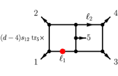
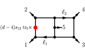
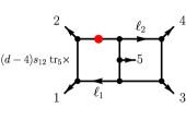
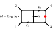
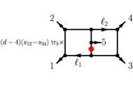
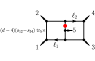
Figure 3: The six parity-odd $(6-2\epsilon)$-dimensional master integrals and their normalization factors. The integrals have no numerators. A red dot indicates that the propagator is “doubled” i.e. raised to a squared power.

The purity of the nine nonplanar double-pentagon integrals we just discussed can be confirmed by evaluating the differential equations at numerical phase-space points and checking the factorization of the dimensional regulator $\epsilon$. For this topology, there are 31 letters ($1\leq\alpha\leq 31$) and 108 master integrals ($1\leq a,b\leq 108$). The 31 square matrices of rational numbers $M_{\alpha}^{ab}$ are determined by performing numerical IBP reductions on a sufficient number of rational phase-space points in a finite field. Details of the reduction procedure will be discussed in the next section, as we used the same implementation for computing the differential equations as we did for reducing the amplitude to the basis of master integrals.

Once the differential equation has been computed, we obtain the symbol of the master integrals by evaluating a single trivial integral to leading order in $\epsilon$, which fixes the overall normalization of the functions, and imposing the first-entry condition Gaiotto:2011dt . Explicit results for the master integrals we use can be found in the ancillary files of ref. Abreu:2018aqd . They satisfy the conjectured second-entry condition Chicherin:2017dob .

4.2 Numerical reduction and analytic reconstruction

Having discussed the evaluation of the master integrals from their differential equations, we now describe the final step in computing the symbol of the $\mathcal{N}\!=\!8\text{ SUGRA}$ amplitude: the reduction of the representation in eq. (4) to our basis of master integrals. Both this step and the calculation of the differential equation discussed above require performing numerical IBP reductions. We now discuss our implementation.

We perform IBP reduction in terms of unitarity cuts and computational algebraic geometry Gluza:2010ws ; Ita:2015tya ; Larsen:2015ped ; Abreu:2017hqn ; Boehm:2018fpv . Once more, we focus on the most challenging topology, the nonplanar double-pentagon in diagram $(c)$ of fig. 1. The reduction is performed on a set of 11 spanning cuts, which are the cuts shown in fig. 4 and their images under the $Z_{2}\times Z_{2}$ symmetry of the diagram (horizontal and vertical flip). Merging the reductions on each of the 11 spanning cuts, we recover the complete IBP reductions for the uncut topology. (A more detailed description of our implementation can be found in ref. Abreu:2018rcw .)

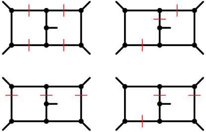
Figure 4: A spanning set of cuts for performing IBP reduction for the nonplanar double pentagon diagram. A cut propagator is indicated by a red line. There are 11 cuts in total, from applying diagram symmetries to the 4 representative cuts shown here.

Unitarity cuts are most natural in the absence of doubled (squared) propagators. However, doubled propagators are present in conventional IBP relations,

$$0=\int d^{d}\ell_{1}\int d^{d}\ell_{2}\sum_{A=1}^{2}\frac{\partial}{\partial\ell_{A}^{\mu}}\frac{v_{A}^{\mu}}{\rho_{1}\rho_{2}\dots\rho_{N}},$$ (42)

because the derivatives can act on the propagator $1/\rho_{i}$. This problem is avoided by choosing vectors $v_{A}^{\mu}$ that satisfy the condition Gluza:2010ws

$$\sum_{A=1}^{2}v_{A}^{\mu}\,\frac{\partial\rho_{i}}{\partial\ell_{A}^{\mu}}=f_{i}\,\rho_{i}\,,$$ (43)

where both $v_{A}^{\mu}$ and $f_{i}$ are required to have polynomial dependence on the components of the loop and external momenta. Finding a full set of $v_{A}^{\mu}$ satisfying eq. (43) is a problem that can be solved by computational algebraic geometry. State-of-the-art algorithms to solve this equation can be found in refs. Abreu:2017hqn ; Boehm:2018fpv ; Abreu:2018rcw , following many earlier devolopments Gluza:2010ws ; Schabinger:2011dz ; Ita:2015tya ; Larsen:2015ped ; Zhang:2016kfo ; Georgoudis:2016wff ; Bern:2017gdk . Avoiding doubled propagators drastically reduces the number of integrals that are present in the linear system of IBP relations, and reduces the computational resources needed for solving the linear system via Gaussian elimination. Further speed-up is achieved by performing IBP reduction in a finite field vonManteuffel:2014ixa ; Peraro:2016wsq ; Maierhoefer:2017hyi ; Abreu:2017hqn ; Smirnov:2019qkx whose modulus is a 10-digit prime number, at numerical rational phase-space points.

We now focus our discussion on the reduction of the amplitude, but exactly the same strategy applies to the construction of the differential equation. IBP reduction is performed separately for each of the top-level topologies $(a)$, $(b)$ and $(c)$ in Fig. 1 and the associated “tower” of sub-topologies. Each diagram in the representation of the amplitude given in eq. (4) is separately reduced to master integrals via IBP reduction. We add the six diagrams and their permutations after replacing the master integrals by their values in terms of symbols. For each of the rational phase-space points where we perform the reduction of the amplitude, the final result of the procedure takes the form,

$$S[M_{5,k}^{(2)}]=\sum^{31}_{\alpha_{1}=1}\!\!\cdots\!\!\sum^{31}_{\alpha_{k}=1}b_{\alpha_{1},\ldots,\alpha_{k}}\ \times\left[W_{\alpha_{1}},\ldots,W_{\alpha_{k}}\right],\quad k=2,3,4\,,$$ (44)

where the coefficients $b_{\alpha_{1},\ldots,\alpha_{k}}$ take numerical values in the finite field. Comparing with eq. (36), it is clear that the $b_{\alpha_{1},\ldots,\alpha_{k}}$ are kinematically dependent, as they depend on the rational functions $r_{j}$.

To finish our calculation, we must extract the coefficients $c^{j}_{\alpha_{1},\ldots,\alpha_{k}}$ in eq. (36) from IBP reductions at sufficiently many phase-space points. Generating the numerical data is the most computationally-intensive part of the calculation, which is nevertheless much more efficient than analytic IBP reduction, for the reasons already highlighted when discussing the construction of differential equations. Since the space of rational functions $r_{j}$ is 45-dimensional, solving the linear system to determine the coefficients $c^{j}_{\alpha_{1},\ldots,\alpha_{k}}$ from numerical evaluations is simple. We first obtain the coefficients in the finite field, and since they are very simple rational numbers this information is sufficient to map them to the field of rational numbers.

We finish with a comment on the application of this procedure to compute the differential equation. The equivalent of the rational functions $r_{j}$ are now the $d\log$-forms $d\log W_{\alpha}$ in eq. (37), which form a 31-dimensional space. The equivalent of the coefficients $c^{j}_{\alpha_{1},\ldots,\alpha_{k}}$ are the entries of the matrices $M_{\alpha}^{ab}$. They are determined in the same way and, as for the amplitude, we find they are simple enough that only a single finite field is necessary. We note that the IBP reductions required for the differential equations are harder to obtain than the ones for the $\mathcal{N}\!=\!8\text{ SUGRA}$ amplitude: the former require reducing integrals with numerators of at least degree 3 in the loop momentum, while the latter only involve integrals with numerators of degree 2.

5 Validation

Scattering amplitudes in gauge and gravity theories obey many well understood factorization formulae that are given in terms of simpler quantities. For example, in special kinematic configurations such as soft and collinear limits, the analytic form of the amplitude can be expressed in terms of universal factors and lower-point amplitudes. Similarly, the divergence structure of loop amplitudes (i.e., the poles in $\epsilon$) can be written in terms of lower-loop amplitudes and universal factors. These degenerations onto simpler configurations provide powerful checks for any new calculation. In the following we shall discuss how our analytic result satisfies all these conditions.

5.1 Divergence structure

On general grounds, the divergences of a scattering amplitude can be broadly separated into two classes—ultraviolet (UV) and infrared (IR). In recent years, understanding the UV structure of supergravity theories has received considerable attention and was partially stimulated by the open question about the potential UV finiteness of $\mathcal{N}\!=\!8\text{ SUGRA}$ in 4 dimensions, which would clearly impact our understanding of quantum gravity on a more fundamental level. The critical dimension in which $\mathcal{N}\!=\!8\text{ SUGRA}$ diverges has now been explicitly calculated through five loops Bern:1998ug ; GravityThreeLoop ; Manifest3 ; N8FourLoop ; ColorKinematics ; Bern:2018jmv . In 4 dimensions, there are various arguments that rule out UV divergences up to at least seven loops GreenDuality ; BossardHoweStellDuality ; BeisertN8 ; Vanhove:2010nf ; Bjornsson:2010wm ; Bjornsson:2010wu ; VanishingVolume . The important aspect for our work here is the fact that the two-loop five-point amplitude only has IR divergences. In comparison to gauge theory, the IR divergence structure of gravity is rather muted. It has been known for a long time that there are no virtual collinear divergences in any quantum theory of gravitation Weinberg:1965nx . Furthermore, it can be shown that the structure of the soft divergences in gravity is completely controlled by the one-loop result, which contains a $1/\epsilon$ pole. Specifically, it can be shown that the one-loop divergence exponentiates SchnitzerN8UniformTrans ; Weinberg:1965nx ; Akhoury:2011kq ; Beneke:2012xa ; Dunbar:1995ed ; Naculich:2011ry ; White:2011yy . In the case of two-loop four-point amplitudes this was explicitly demonstrated in ref. BoucherVeronneau:2011qv .

In order to check the divergence structure of the two-loop five-point amplitude, we therefore begin by recalling the one-loop result Bern:1998sv ,

$$M^{(1)}_{5}=\frac{1}{2}\sum_{S_{5}}\left(\frac{1}{4}\beta_{123(45)}\,I^{d=4\raisebox{0.75pt}{\scalebox{0.75}{$\,-\,$}}2\epsilon}_{123(45)}-\frac{1}{10}\frac{[12][23][34][45][51]}{\langle 12\rangle\langle 23\rangle\langle 34\rangle\langle 45\rangle\langle 51\rangle}(-2\epsilon)I^{d=6\raisebox{0.75pt}{\scalebox{0.75}{$\,-\,$}}2\epsilon}_{12345}\right)\,,$$ (45)

where the rational factors of $1/4$ and $1/10$ inside the $S_{5}$ permutation sum remove over-counting, and

$$\beta_{123(45)}=-\frac{[12]^{2}[23]^{2}[45]}{\langle 14\rangle\langle 15\rangle\langle 34\rangle\langle 35\rangle\langle 45\rangle}\,.$$ (46)

$I^{d=4\raisebox{0.75pt}{\scalebox{0.75}{$\,-\,$}}2\epsilon}_{123(45)}$ is the one-mass scalar box integral in $4-2\epsilon$ dimensions, and $I^{d=6\raisebox{0.75pt}{\scalebox{0.75}{$\,-\,$}}2\epsilon}_{12345}$ is the massless pentagon integral in $6-2\epsilon$ dimensions normalized as follows:

$$I^{d=4\raisebox{0.75pt}{\scalebox{0.75}{$\,-\,$}}2\epsilon}_{123(45)} =e^{\epsilon\gamma_{E}}\int\!\!\frac{d^{4\raisebox{0.75pt}{\scalebox{0.75}{$\,-\,$}}2\epsilon}\ell}{i\pi^{2\raisebox{0.75pt}{\scalebox{0.75}{$\,-\,$}}\epsilon}}\frac{1}{\ell^{2}(\ell\raisebox{0.75pt}{\scalebox{0.75}{$\,-\,$}}k_{1})^{2}(\ell\raisebox{0.75pt}{\scalebox{0.75}{$\,-\,$}}k_{1}\raisebox{0.75pt}{\scalebox{0.75}{$\,-\,$}}k_{2})^{2}(\ell\raisebox{0.75pt}{\scalebox{0.75}{$\,+\,$}}k_{4}\raisebox{0.75pt}{\scalebox{0.75}{$\,+\,$}}k_{5})^{2}}\,,$$ (47)

$$I^{d=6\raisebox{0.75pt}{\scalebox{0.75}{$\,-\,$}}2\epsilon}_{12345} =e^{\epsilon\gamma_{E}}\int\!\!\frac{d^{6\raisebox{0.75pt}{\scalebox{0.75}{$\,-\,$}}2\epsilon}\ell}{i\pi^{3\raisebox{0.75pt}{\scalebox{0.75}{$\,-\,$}}\epsilon}}\frac{1}{\ell^{2}(\ell\raisebox{0.75pt}{\scalebox{0.75}{$\,-\,$}}k_{1})^{2}(\ell\raisebox{0.75pt}{\scalebox{0.75}{$\,-\,$}}k_{1}\raisebox{0.75pt}{\scalebox{0.75}{$\,-\,$}}k_{2})^{2}(\ell\raisebox{0.75pt}{\scalebox{0.75}{$\,+\,$}}k_{4})^{2}(\ell\raisebox{0.75pt}{\scalebox{0.75}{$\,+\,$}}k_{4}\raisebox{0.75pt}{\scalebox{0.75}{$\,+\,$}}k_{5})^{2}}\,.$$ (48)

The box integral is known to all orders in $\epsilon$ Bern:1993kr and the symbol of the pentagon integral can be computed to any order in $\epsilon$ with the techniques of Abreu:2017mtm ; Abreu:2017enx or by direct integration with HyperInt Panzer:2014caa . In ancillary files, we provide symbols for the pure functions (${\cal I}$) obtained by normalizing these integrals by their leading singularities,

$$\mathcal{I}^{d=4\raisebox{0.75pt}{\scalebox{0.75}{$\,-\,$}}2\epsilon}_{123(45)}\equiv s_{12}s_{23}I^{d=4\raisebox{0.75pt}{\scalebox{0.75}{$\,-\,$}}2\epsilon}_{123(45)}\,,\qquad\mathcal{I}^{d=6\raisebox{0.75pt}{\scalebox{0.75}{$\,-\,$}}2\epsilon}_{12345}\equiv-\text{tr}_{5}\,I^{d=6\raisebox{0.75pt}{\scalebox{0.75}{$\,-\,$}}2\epsilon}_{12345}\,.$$ (49)

Despite the presence of $1/\epsilon^{2}$ soft-collinear divergences in individual box integrals, they cancel in the sum to give

$$M^{(1)}_{5}=\frac{1}{\epsilon}\left[\sum_{i<j=1}^{5}s_{ij}\log s_{ij}\right]M^{(0)}_{5}+M^{(1),0}_{5}\,+O(\epsilon),$$ (50)

where $M_{5}^{(1),0}$ is the ${\cal O}(\epsilon^{0})$ term in the one-loop amplitude. Finally, at two loops, the divergent pieces are dictated by exponentiation in terms of the square of the one-loop amplitude:

$$M^{(2),\text{div}}_{5}=\left.\frac{1}{2}\left[\frac{M^{(1)}_{5}}{M^{(0)}_{5}}\right]^{2}\!\!\times M^{(0)}_{5}\right|_{\text{pole-terms}}\,.$$ (51)

Inserting the symbols of the relevant one-loop integrals and comparing against the divergences of our two-loop result we find perfect agreement. The factor predicting the pole structure permits many natural extensions that include different finite pieces. What the “ideal” choice is an interesting question which we will discuss in section 6.

5.2 Soft factorization

Gravity amplitudes, similarly to gauge amplitudes, have a universal factorization property when a single graviton becomes much softer than the remaining gravitons. At tree level, the general factorization when the $n^{\rm th}$ graviton becomes soft, $k_{n}\to 0$, is Weinberg:1965nx ; Berends:1988zp ,

$$M_{n}^{(0)}(1,\ldots,n\raisebox{0.75pt}{\scalebox{0.75}{$\,-\,$}}1,n^{\pm})\ \mathop{\Longrightarrow}^{k_{n}\to 0}\ \mathcal{S}_{n}^{\pm}\times M_{n\raisebox{0.75pt}{\scalebox{0.75}{$\,-\,$}}1}^{(0)}(1,\ldots,n\raisebox{0.75pt}{\scalebox{0.75}{$\,-\,$}}1)\,,$$ (52)

where the positive-helicity soft factor is

$$\mathcal{S}_{n}^{+}=\frac{-1}{\langle 1n\rangle\langle n\,n\raisebox{0.75pt}{\scalebox{0.75}{$\,-\,$}}1\rangle}\sum_{i=2}^{n\raisebox{0.75pt}{\scalebox{0.75}{$\,-\,$}}2}\frac{\langle 1i\rangle\langle i\,n\raisebox{0.75pt}{\scalebox{0.75}{$\,-\,$}}1\rangle[in]}{\langle in\rangle}\,.$$ (53)

Naively, the definition of the soft factor $\mathcal{S}_{n}^{+}$ seems to pick out two further special legs, $n-1$ and $1$. One can however show that this term is independent of that particular choice, which will become important momentarily. In ref. Bern:1998sv it was shown that there are no loop corrections to the leading soft factorization for gravity. That is,

$$M_{n}^{(1)}(1,\ldots,n\raisebox{0.75pt}{\scalebox{0.75}{$\,-\,$}}1,n^{\pm})\ \mathop{\Longrightarrow}^{k_{n}\to 0}\ \mathcal{S}_{n}^{\pm}\times M_{n\raisebox{0.75pt}{\scalebox{0.75}{$\,-\,$}}1}^{(1)}(1,\ldots,n\raisebox{0.75pt}{\scalebox{0.75}{$\,-\,$}}1)\,,$$ (54)

$$M_{n}^{(2)}(1,\ldots,n\raisebox{0.75pt}{\scalebox{0.75}{$\,-\,$}}1,n^{\pm})\ \mathop{\Longrightarrow}^{k_{n}\to 0}\ \mathcal{S}_{n}^{\pm}\times M_{n\raisebox{0.75pt}{\scalebox{0.75}{$\,-\,$}}1}^{(2)}(1,\ldots,n\raisebox{0.75pt}{\scalebox{0.75}{$\,-\,$}}1)\,.$$ (55)

We will test our result for the five-point amplitude against eq. (55) for $n=5$.

First, we determine the soft behavior of the 31 symbol letters in eq. (111). We parametrize the approach to the $k_{5}\to 0$ soft limit with a parameter $\delta\to 0$. We then rewrite the $x_{i}$ momentum-twistor parametrization of ref. Badger:2013gxa (see Appendix A for more details) as

$$\begin{split}x_{1}&=s,\quad x_{2}=sx,\quad x_{3}=-\frac{sx}{1-z}\,,\\ x_{4}&=1+\delta\,\frac{x+\overline{z}}{1-\overline{z}}\,,\quad x_{5}=1+\delta\biggl{[}1+\frac{x+\overline{z}}{1-\overline{z}}\biggr{]}\,,\end{split}$$ (56)

where $s=s_{12}$, $x=s_{23}/s_{12}$, $z=\langle 14\rangle\langle 35\rangle/(\langle 34\rangle\langle 15\rangle)$, and $\overline{z}=[14][35]/([34][15])$ at leading order in the $\delta\to 0$ limit. The set of 14 letters obtained in this limit are

$$\begin{split}&\{s,x,1+x\}\ \cup\ \{\delta,z,1-z,x+z,\overline{z},1-\overline{z},x+\overline{z}\}\\ &\cup\ \{x+z+\overline{z}-z\overline{z},\ x(z+\overline{z}-1)+z\overline{z},\ x+z\overline{z},\ z-\overline{z}\}\,.\end{split}$$ (57)

In the soft limit of the two-loop five-point $\mathcal{N}=8$ supergravity amplitude, it follows from eq. (55) that only the subset $\{s,x,1+x\}$ should appear, after taking into account the behavior of the rational prefactors. In the soft limit of the two-loop five-point $\mathcal{N}=4$ super-Yang-Mills amplitude, the second set of letters can also appear in subleading-color terms, and is consistent with a computation of two-loop soft-gluon emission using Wilson lines LanceToAppear .

To analyze the soft limit of our five-point amplitude, we perform the substitution (56) within the symbol entries, and refactorize the symbol on the set of letters in (57). Then we consider the soft behavior of the rational prefactors.

In the case we are interested in, $n=5$, the soft factor (53) has only two terms,

$${\cal S}\ \equiv\ {\cal S}_{5}^{+}\ =\ {\cal P}_{14}^{2}+{\cal P}_{14}^{3}\,,$$ (58)

where

$${\cal P}_{jk}^{i}\equiv-\frac{\langle ji\rangle\langle ki\rangle[i5]}{\langle j5\rangle\langle k5\rangle\langle i5\rangle}\,.$$ (59)

In the soft limit, the little group transformation properties imply that all the rational factors $r_{j}$ in eq. (9) are either nonsingular or become proportional to the four-point amplitude multiplied by one of these partial soft factors ${\cal P}_{jk}^{i}$. Because (59) is symmetric in $j$ and $k$, and $i,j,k\in\{1,2,3,4\}$, there are 12 such factors. However, they sum in six pairs to the soft factor,

$${\cal P}_{jk}^{i_{1}}+{\cal P}_{jk}^{i_{2}}={\cal S},$$ (60)

where $i_{1,2}\not\in\{j,k,5\}$. Equation (60) reflects the fact that any two gravitons can play the role of gravitons 1 and $n-1$ in (53).

There is one more useful identity among the partial soft factors,

$$s_{13}({\cal P}_{24}^{3}-{\cal P}_{13}^{4})=s_{12}({\cal P}_{12}^{4}-{\cal P}_{34}^{2})-(s_{15}+s_{45})\mathcal{P}^{1}_{23}$$ (61)

plus all equations obtained by permuting legs $\{1,2,3,4\}$. The second term on the right-hand side can be dropped in the soft limit.

Using the identities (60) and (61), and the symbol substitutions mentioned above, we find that all letters except $\{s,x,1+x\}$ drop out of the soft limit. Furthermore, the limit is proportional to the symbol of the four-point $\mathcal{N}=8$ supergravity amplitude given in ref. BoucherVeronneau:2011qv (see also refs. SchnitzerN8UniformTrans ; QueenMaryN8UniformTrans ). That is, the five-point amplitude precisely satisfies the soft limit (55).

5.3 Collinear factorization

The behavior of gravity amplitudes as two gravitons $a$ and $b$ become collinear is also universal and well established Bern:1998xc ,

$$M_{n}^{(0)}(1,\ldots,a,b,\ldots,n)\ \mathop{\Longrightarrow}^{k_{a}||k_{b}}\ {\rm Split}^{\rm grav}(\tau,a,b)\times M_{n-1}^{(0)}(1,\ldots,P,\ldots,n)\,.$$ (62)

In eq. (62) we define the common momentum $k_{P}=k_{a}+k_{b}$, and write $k_{a}\approx\tau k_{P}$, $k_{b}\approx(1-\tau)k_{P}$ with the splitting fraction $\tau$ for the longitudinal momentum. In contrast to the case of gauge theory, for real collinear kinematics, the amplitude does not diverge in the limit. Rather, ${\rm Split}^{\rm grav}(\tau,a,b)$ is a pure phase, containing dependence on the azimuthal angle as the two nearly-collinear gravitons are rotated around the axis formed by the sum of their momenta. This behavior stems from a factor of $[ab]/\langle ab\rangle$ in the amplitude (or $\langle ab\rangle/[ab]$, depending on the helicity configuration) as legs $a$ and $b$ become collinear.

At tree level, the form of the gravitational collinear splitting factor can be understood from the KLT relations KLT to originate from a product of two singular gauge-theory splitting amplitudes and a factor of $s_{ab}$ in the numerator Bern:1998sv ,

$${\rm Split}^{\rm grav}_{-2\lambda}(\tau,a^{2\lambda_{a}},b^{2\lambda_{b}})=-s_{ab}\times[{\rm Split}^{\rm YM}_{-\lambda}(\tau,a^{\lambda_{a}},b^{\lambda_{b}})]^{2}\,.$$ (63)

Here $\lambda_{a}$ and $\lambda_{b}$ are the helicities of the two external gluons for both of the gauge copies. The sums of their helicities, $2\lambda_{a}$ and $2\lambda_{b}$, are the external graviton helicities, and similarly for the intermediate helicities $\lambda$ and $2\lambda$.

For the five-point amplitude in $\mathcal{N}=8$ supergravity, it is convenient to take all collinear helicities to be positive, $\lambda_{a}=\lambda_{b}=\lambda=+$, and we obtain,

$${\rm Split}^{\rm grav}_{-}(\tau,a^{+},b^{+})\ =\ -{1\over\tau(1-\tau)}{\left[a\,b\right]\over\left\langle a\,b\right\rangle}\,.$$ (64)

As in the case of soft factorization, there are no loop corrections to the splitting amplitude Bern:1998sv , so the one- and two-loop amplitudes behave as,

$$M_{n}^{(1)}(1,\ldots,a,b,\ldots,n)\ \mathop{\Longrightarrow}^{k_{a}||k_{b}}\ {\rm Split}^{\rm grav}(\tau,a,b)\times M_{n-1}^{(1)}(1,\ldots,P,\ldots,n)\,,$$ (65)

$$M_{n}^{(2)}(1,\ldots,a,b,\ldots,n)\ \mathop{\Longrightarrow}^{k_{a}||k_{b}}\ {\rm Split}^{\rm grav}(\tau,a,b)\times M_{n-1}^{(2)}(1,\ldots,P,\ldots,n)\,.$$ (66)

We will test the collinear behavior of the two-loop five-graviton amplitude against (66), with splitting amplitude (64). Since the (super-)amplitude is Bose symmetric, it does not matter which two legs we take to be parallel. For convenience we discuss the same limit we studied for the two-loop five-point $\mathcal{N}=4$ SYM amplitude Abreu:2018aqd , $k_{2}||k_{3}$, i.e. $a=2$ and $b=3$. The two-loop four-point $\mathcal{N}=8$ supergravity amplitude SchnitzerN8UniformTrans ; QueenMaryN8UniformTrans ; BoucherVeronneau:2011qv should be evaluated with momenta $(k_{1},k_{P},k_{4},k_{5})$.

The analysis of the symbol proceeds exactly as in ref. Abreu:2018aqd . Employing the $x_{i}$ variables of ref. Badger:2013gxa , we let

$$x_{1}\mapsto s\tau\,,\quad x_{2}\mapsto cs\delta\,,\quad x_{3}\mapsto r_{2}cs\delta\,,\quad x_{4}\mapsto\delta\,,\quad x_{5}\mapsto-\frac{1}{c\delta}\,,$$ (67)

where $s=s_{45}$ and $r_{2}=s_{15}/s_{45}$ characterize the four-point kinematics, $c\sim[23]/\langle 23\rangle$ corresponds to an azimuthal phase, and $\delta=\sqrt{s_{23}/(s\ c)}$ vanishes in the collinear limit. We expand the 31 letter alphabet in the collinear limit to leading order in $\delta$, finding 14 multiplicatively independent letters in the collinear limit: 7 physical letters $\{\delta,\ s,\ \tau,\ 1-\tau,\ r_{2},\ 1+r_{2},\ c\}$ and 7 spurious letters that are in neither the splitting amplitude nor the four-point amplitude; hence they must not contribute to the universal limit.

After refactorizing the amplitude on these symbol letters, we choose numerical kinematics near the collinear limit, and take the difference between evaluations at two different points corresponding to an azimuthal rotation of the two collinear gravitons. Taking this difference removes non-universal terms that would otherwise be of the same order, and the results are numerically consistent with the expected factorization (66). Alternatively, one can use complexified momenta and perform two non-overlapping BCFW shifts BCFW , e.g. $\lambda_{2}\to\lambda_{2}+z\lambda_{4},\ \widetilde{\lambda}_{4}\to\widetilde{\lambda}_{4}-z\widetilde{\lambda}_{2}$ and $\lambda_{5}\to\lambda_{5}+w\lambda_{3},\ \widetilde{\lambda}_{3}\to\widetilde{\lambda}_{3}-w\widetilde{\lambda}_{5}$ and then solve $\langle 23\rangle=\epsilon_{1}\,,[23]=\epsilon_{2}$ in terms of $z$ and $w$. Expanding around $\epsilon_{1}=0$ then allows one to check that the pole term is proportional to $\epsilon_{2}$, which was used as an independent check of the collinear factorization property of our result.

6 Structure of results

The purpose of this section is to provide some insight into the structure of the amplitude we have computed. First we define a prescription for removing the infrared divergences, which also cleans up the finite hard remainder. Then we write the remainder $R_{5}^{(2)}$ in a manifestly symmetric form, which requires only summing over permutations of a single rational structure, multiplied by a single weight 4 function $h$. We note that the finite quantity $h$ cannot be written only in terms of the classical polylogarithms $\log$, $\operatorname{Li}_{2}$, $\operatorname{Li}_{3}$ and $\operatorname{Li}_{4}$, but also requires the function $\operatorname{Li}_{2,2}$ (this can be checked with the procedure described in ref. Goncharov:2010jf ). We characterize the properties of $h$ in terms of its final entries and the weight-3 odd parts of its derivatives. We go on to characterize the full space of 45 functions in the (unsubtracted) $\mathcal{N}\!=\!8\text{ SUGRA}$ amplitude, and compare it with its cousin, the corresponding $\mathcal{N}\!=\!4\text{ SYM}$ amplitude, also at the level of their derivatives (coproducts). In the course of doing this, we discovered linear relations between components of the $\mathcal{N}\!=\!4\text{ SYM}$ five-point amplitude at one and two loops.

One interesting “global” property of the $\mathcal{N}\!=\!8\text{ SUGRA}$ amplitude is that the letter $W_{31}$ does not appear at all, neither in the unsubtracted amplitude nor in the subtracted hard function to be described shortly. It does appear in the $\mathcal{N}\!=\!4\text{ SYM}$ amplitude Abreu:2018aqd ; Chicherin:2018yne , but this appears to be linked solely to its contribution to the ${\cal O}(\epsilon^{2})$ part of the $(6-2\epsilon)$-dimensional pentagon integral, which is required at two loops for infrared subtractions in $\mathcal{N}\!=\!4\text{ SYM}$, but not in $\mathcal{N}\!=\!8\text{ SUGRA}$ because of the milder IR divergence structure.

6.1 A symmetric form of the hard remainder $R^{(2)}_{5}$

As mentioned around eq. (51), in order to remove the infrared divergences from the two-loop amplitude, one could simply subtract the full square of the one-loop amplitude. That is, one could define

$$\begin{split}\tilde{R}_{5}^{(2)}&\equiv M_{5}^{(2)}-\frac{1}{2}\left[\frac{M^{(1)}_{5}}{M^{{(0)}}_{5}}\right]^{2}\!\!\times M^{{(0)}}_{5}\\ &=M_{5}^{(2)}-\frac{1}{2}\left[\frac{1}{\epsilon}\Bigl{(}\sum_{i<j}s_{ij}\log s_{ij}\Bigr{)}+\frac{M_{5}^{(1),0}}{M^{{(0)}}_{5}}+\epsilon\,\frac{M_{5}^{(1),1}}{M^{{(0)}}_{5}}\right]^{2}\!\!\times M^{{(0)}}_{5}\ +\ {\cal O}(\epsilon)\\ &=M_{5}^{(2)}-\Bigl{(}\sum_{i<j}s_{ij}\log s_{ij}\Bigr{)}\times\left[\frac{1}{2\epsilon^{2}}\Bigl{(}\sum_{i<j}s_{ij}\log s_{ij}\Bigr{)}M^{{(0)}}_{5}+\frac{1}{\epsilon}M_{5}^{(1),0}+M_{5}^{(1),1}\right]\\ &\hskip 36.98866pt\hbox{}-\frac{\left[M_{5}^{(1),0}\right]^{2}}{2\,M^{{(0)}}_{5}}\ +\ {\cal O}(\epsilon),\end{split}$$ (68)

where $M_{5}^{(1),0}$ and $M_{5}^{(1),1}$ are the ${\cal O}(\epsilon^{0})$ and ${\cal O}(\epsilon^{1})$ terms in the one-loop amplitude. However, doing this full subtraction would enlarge the space of rational structures required. The issue is with the final term. The tree amplitude $M^{{(0)}}_{5}$ is proportional to $\text{tr}_{5}$, see eq. (2), and appears in the denominator. Within the square of $M_{5}^{(1),0}$, the products of different permutations of the box coefficient (46), after dividing by $M^{{(0)}}_{5}$, cannot be expressed in terms of the 45 rational structures of eqs. (31) and (32). Instead, we simply omit this last term and define

$$R_{5}^{(2)}\equiv M_{5}^{(2)}-\Bigl{(}\sum_{i<j}s_{ij}\log s_{ij}\Bigr{)}\times\left[\frac{1}{2\epsilon^{2}}\Bigl{(}\sum_{i<j}s_{ij}\log s_{ij}\Bigr{)}M^{{(0)}}_{5}+\frac{1}{\epsilon}M_{5}^{(1),0}+M_{5}^{(1),1}\right]\,.$$ (69)

The ${\cal O}(\epsilon)$ terms in the one-loop amplitude induce a shift in the finite terms of the two-loop amplitude. In particular, there is a factor of $\text{tr}_{5}$ in the denominator of the coefficient of the $d=6$ pentagon integral, which cancels precisely against the $1/\text{tr}_{5}$-containing contributions to the bare two-loop amplitude. After this cancellation, there are only 40 linearly independent rational structures, multiplied by 40 linearly independent weight 4 transcendental functions.

We remark that this cancellation of more complicated structures, which are associated with $d$-dimensional cuts rather than 4 dimensional ones, is reminiscent of what was observed for the six-point amplitude in planar $\mathcal{N}\!=\!4\text{ SYM}$ Bern:2008ap . In that case, integrals containing $\mu^{2}$ factors (extra-dimensional components of the loop momentum) appeared at two loops and at ${\cal O}(\epsilon)$ in the one-loop amplitude, but cancelled out from the remainder function. The physical importance of the finite remainder at two loops has also been stressed in the context of constructing finite cross sections Weinzierl:2011uz . The conclusion is that the $1/\text{tr}_{5}$ rational structures, originating from $d$-dimensional leading singularities, see eq. (32), should be thought of as unphysical and dependent on the use of dimensional regularization.

The 40 linearly independent rational structures appearing in the hard function do not fall into nice orbits under $S_{5}$. Consider for example, the structure

$$r_{0}=\frac{[23][34][45][51]}{\langle 13\rangle\langle 14\rangle\langle 15\rangle\langle 23\rangle\langle 24\rangle\langle 25\rangle}\,.$$ (70)

It is invariant under the $Z_{2}$ symmetry that exchanges $1\leftrightarrow 2$ and $3\leftrightarrow 5$. So the action of $S_{5}$ on $r_{0}$ generates $120/2=60$ similar structures, only 40 of which are linearly independent.

In order to provide a symmetric form for the hard remainder $R^{(2)}_{5}$, we find a linear combination $h$ of the 40 weight 4 functions which is symmetric under the same $Z_{2}$ as $r_{0}$, and write $R^{(2)}_{5}$ as a sum over the 60 permutations in $S_{5}/Z_{2}$,

$$R^{(2)}_{5}=\sum_{\sigma\in S_{5}/Z_{2}}r_{0}(\sigma)\,h(\sigma).$$ (71)

Requiring that $R^{(2)}_{5}$ be the same as in the original linearly-independent 40-term representation leaves a 6 parameter space of solutions. We pick a particular solution in this space in order to simplify $h$, as we shortly explain. The symbol of $h$ contains 26,012 terms and is provided in the ancillary file remainder_h.txt.

We can characterize $h$ via its derivative, or more technically the $\{3,1\}$ component of its coproduct, in much the same way that we characterized the pure function $g_{234}^{\text{DT}}$ appearing in the double-trace coefficient of the $\mathcal{N}\!=\!4\text{ SYM}$ amplitude Abreu:2018aqd . We first remark that the parity odd part of $h$, like the odd part of $g_{234}^{\text{DT}}$, has vanishing final entries for all letters of the form $s_{ij}-s_{kl}$ (letters 6 to 15 and 21 to 25, see appendix A.1). In addition, the weight 3 odd functions appearing in the $\{3,1\}$ coproduct component are all linear combinations of permutations of the pure $d=6$ pentagon integral, the $\mathcal{I}^{d=6}_{5}$ defined in eq. (49), whose symbol we give in an ancillary file (we use the same conventions as in ref. Abreu:2018aqd ). However, in contrast to $g_{234}^{\text{DT}}$, $h$ does not contain letter 31 at all. By an appropriate choice of solution in the 6 parameter space, we find that the final entries for letters 17 and 19 vanish as well, for the odd part, $h^{\text{odd}}$. We write the parity-odd part of its derivative as,

$$\hskip 2.0pt\partial_{x_{i}}\left[h^{\text{odd}}\right]\big{|}_{\text{odd}}=\sum^{12}_{j=1}\sum_{\alpha_{1}}\mathcal{I}^{d=6}_{5}(\Sigma_{j})\ m_{j\alpha_{1}}\ \frac{\partial\log W_{\alpha_{1}}}{\partial x_{i}}\,,\vspace{-3.5pt}$$ (72)

where $j$ labels the 12 inequivalent permutations of the $d=6$ pentagon integral,

$$\begin{split}\Sigma_{j}&\in\{\{12543\},\{12453\},\{13524\},\{12534\},\{13254\},\{12354\},\\ &{\color[rgb]{1,1,1}.}\hskip 17.07182pt\{14325\},\{13425\},\{14235\},\{12435\},\{13245\},\{12345\}\},\end{split}$$ (73)

and $\alpha_{1}\in\{1,\!...,\!5\}\cup\{16,\!...,\!20\}\cup\{31\}$ are the nonzero final entries for $g_{234}^{\text{DT}}$.

In these conventions, the matrix $m_{j\alpha_{1}}$ corresponding to $h^{\text{odd}}$ is

$$\hskip-19.91684ptm_{j\alpha_{1}}=\frac{1}{12}\left(\begin{array}[]{rrrrrrrrrrr}-3&-2&2&2&-2&1&0&1&0&1&0\\[2.0pt] 3&1&-1&-3&0&1&0&-1&0&0&0\\[2.0pt] -3&-2&0&0&-2&1&0&5&0&1&0\\[2.0pt] 3&0&-3&-1&1&0&0&-1&0&1&0\\[2.0pt] 3&0&0&-2&4&-3&0&-3&0&1&0\\[2.0pt] -3&-1&1&3&0&-1&0&1&0&0&0\\[2.0pt] -3&2&-1&3&-3&2&0&3&0&-3&0\\[2.0pt] 3&4&-2&0&0&1&0&-3&0&-3&0\\[2.0pt] 3&-1&0&0&-1&2&0&-5&0&2&0\\[2.0pt] -3&0&3&1&-1&0&0&1&0&-1&0\\[2.0pt] -3&-3&3&-1&2&-3&0&3&0&2&0\\[2.0pt] 3&2&-2&-2&2&-1&0&-1&0&-1&0\\[2.0pt] \end{array}\right)\,.$$ (86)

This matrix has rank 5, so the derivative contains only five independent combinations of final entries, and five independent combinations of $d=6$ pentagon permutations.

Similarly, we expand the odd part of the derivative of the parity even part of $h$ as,

$$\partial_{x_{i}}\left[h^{\text{even}}\right]\big{|}_{\text{odd}}=\sum^{12}_{j=1}\sum_{\alpha_{2}}\mathcal{I}^{d=6}_{5}(\Sigma_{j})\ n_{j\alpha_{2}}\ \frac{\partial\log W_{\alpha_{2}}}{\partial x_{i}}\,,$$ (87)

where $\alpha_{2}\in\{26,\ldots,30\}$ runs only over the five odd letters. The matrix $n_{j\alpha_{2}}$ for $h^{\text{even}}$ is given by

$$\hskip-19.91684ptn_{j\alpha_{2}}=\frac{1}{12}\left(\begin{array}[]{rrrrr}0&1&0&1&1\\[2.0pt] 0&-1&0&0&1\\[2.0pt] 0&1&0&-1&-1\\[2.0pt] 0&-1&0&1&0\\[2.0pt] 0&-1&0&-1&1\\[2.0pt] 0&1&0&0&-1\\[2.0pt] 0&1&0&1&0\\[2.0pt] 0&-1&0&1&-1\\[2.0pt] 0&-1&0&0&0\\[2.0pt] 0&1&0&-1&0\\[2.0pt] 0&1&0&0&1\\[2.0pt] 0&-1&0&-1&-1\\[2.0pt] \end{array}\right)\,.$$ (100)

This matrix has rank 3, corresponding to the vanishing of the final entries 26 and 28.

6.2 Counting functions for $\mathcal{N}\!=\!8\text{ SUGRA}$ and $\mathcal{N}\!=\!4\text{ SYM}$

It is interesting to compare the spaces of transcendental functions for $\mathcal{N}\!=\!8\text{ SUGRA}$ and $\mathcal{N}\!=\!4\text{ SYM}$. Before doing so for the two-loop five-point case of interest, we review the situation for lower numbers of loops and/or legs, concentrating on the order ${\cal O}(\epsilon^{0})$ terms of weight 2 at one loop and weight 4 at two loops.

For the one-loop four-point amplitudes in both theories Green:1982sw , the space is three-dimensional, and very simple in terms of the Mandelstam variables $s,t,u$ (omitting factors of $\log\mu^{2}$):

$$\{\log s\,\log t,\ \log t\,\log u,\ \log u\,\log s\}\,.$$ (101)

The finite part of the leading-color one-loop five-point $\mathcal{N}\!=\!4\text{ SYM}$ amplitude contains only logarithms Bern:1993mq

$$V_{5}\ =\ \sum_{j=1}^{5}\Biggl{[}-\frac{1}{2}\log^{2}s_{j,j+1}+\log\left(\frac{s_{j,j+1}}{s_{j+1,j+2}}\right)\log\left(\frac{s_{j+2,j-2}}{s_{j-2,j-1}}\right)+\zeta_{2}\Biggr{]}\,.$$ (102)

The function is invariant under the dihedral $D_{5}$ symmetry of planar amplitudes. In the full-color amplitude, it appears in 12 nontrivial permutations labeled by $S_{5}/D_{5}$. Subleading-color contributions are also obtained from particular permutations of this function Bern:1990ux . The linear span of the 12 permutations of eq. (102) is an 11-dimensional space. Thus there is one linear relation among the 12 permutations of $V_{5}$,

$$\begin{split}&V_{5}[12345]+V_{5}[12453]+V_{5}[13254]+V_{5}[13425]+V_{5}[14235]+V_{5}[14352]\\ -&V_{5}[12435]-V_{5}[12354]-V_{5}[13245]-V_{5}[13452]-V_{5}[14325]-V_{5}[14253]=0,\end{split}$$ (103)

corresponding to the totally antisymmetric combination of the twelve functions. This relation also holds for the $1/\epsilon$ pole terms as well. It can be derived by representing $V_{5}$ as a cyclic sum of one-mass box integrals, and using the $Z_{2}\times Z_{2}$ symmetry of each such box integral.

What about the one-loop five-point $\mathcal{N}\!=\!8\text{ SUGRA}$ amplitude? From eq. (45), the amplitude contains a sum over one-mass box integrals, so it might be expected to contain the dilogarithms present in the box integral Bern:1993kr . On the other hand, the same could be said for the $\mathcal{N}\!=\!4\text{ SYM}$ amplitude, where from eq. (102) they have long been known to cancel. We find that the dilogarithms all cancel from the one-loop five-point $\mathcal{N}\!=\!8\text{ SUGRA}$ amplitude as well. (As far as we know, this feature was not recognized before, even though this amplitude has been available for over 20 years Bern:1998sv .) In fact, of the 30 permutations of the box coefficient $\beta_{123(45)}$ in eq. (46), only 10 are linearly independent. The coefficient of one of these 10 rational structures is,

$$\frac{1}{2}\log^{2}\left(\frac{s_{41}}{s_{52}}\right)-\frac{1}{2}\log^{2}\left(\frac{s_{51}}{s_{24}}\right)+\log s_{12}\,\log\left(\frac{s_{52}s_{41}}{s_{51}s_{24}}\right)+\log\left(\frac{s_{34}}{s_{35}}\right)\log\left(\frac{s_{51}s_{41}}{s_{52}s_{24}}\right)\,.$$ (104)

Its images under the 30 permutations in $S_{5}/(Z_{2}\times Z_{2})$ span a 10 dimensional space, which is entirely contained within the 11-dimensional space provided by the $V_{5}$ functions for $\mathcal{N}\!=\!4\text{ SYM}$. So by this measure, $\mathcal{N}\!=\!8\text{ SUGRA}$ is slightly simpler than $\mathcal{N}\!=\!4\text{ SYM}$.

Next we turn to the two-loop four-point amplitude. How many functions should we expect in $\mathcal{N}\!=\!4\text{ SYM}$? For a given color ordering, there is one planar amplitude, because only a single Parke-Taylor factor appears at leading color. There are 3 distinct orderings of a single trace, so there are really 3 planar functions. In the full-color amplitude, group theory implies that the subleading-color single-trace coefficients can be traded for the double-trace coefficients, or vice versa, and only two of the three of these are independent Bern:2002tk . Also, there are two Parke-Taylor structures in the four-point case, given the one Kleiss-Kuijf ($U(1)$ decoupling) relation KleissKuijf . So we expect $2\times 2=4$ nonplanar functions, for a total of $3+4=7$. Inspecting the actual $\mathcal{N}\!=\!4\text{ SYM}$ answer BRY ; SchnitzerN8UniformTrans , there are 7 independent functions. So there are no mysterious relations like eq. (103) at two loops and four points. There are 3 functions associated with the $\mathcal{N}\!=\!8\text{ SUGRA}$ two-loop four-point amplitude, with relative prefactors $s^{2}$, $t^{2}$, $u^{2}$ (or $st$, $tu$, $us$). These three functions are contained within the space of $\mathcal{N}\!=\!4\text{ SYM}$ functions. This property was anticipated by a relation found in ref. SchnitzerN8UniformTrans between subleading-color $\mathcal{N}=4$ and $\mathcal{N}=8$ amplitudes, although there are still rational factors inhabiting this relation.

Finally, we turn to the two-loop five-point amplitudes. We need forty-five linearly independent rational structures $r_{j}$ to describe the full unsubtracted amplitude $M^{(2)}_{5}$ in $\mathcal{N}=8$ supergravity. The weight-4 functions that multiply these 45 structures at ${\cal O}(\epsilon^{0})$ are all linearly independent. As discussed in the previous subsection, if we perform the infrared subtraction defined in eq. (69) to remove the pole terms that are proportional to “$s\log s$” times the one-loop amplitude, and if we also include in this subtraction the ${\cal O}(\epsilon)$ terms in the one loop amplitude, then the ${\cal O}(\epsilon^{0})$ terms in the amplitude are shifted. This remainder function has only 40 rational structures, and the corresponding 40 functions are linearly independent.

We can also compare the functions for $\mathcal{N}\!=\!8\text{ SUGRA}$ with the corresponding number for $\mathcal{N}\!=\!4\text{ SYM}$ Abreu:2018aqd ; Chicherin:2018yne . First, we need to understand how many functions there are in the latter amplitude. Naively, there are 72 such functions. The counting is as follows: The planar (BDS) amplitude has a single pure function $M^{\text{BDS}}$ multiplying a single Parke-Taylor factor. As the coefficient of a single trace structure, $\text{tr}[T^{a_{1}}\cdots T^{a_{5}}]\raisebox{0.75pt}{\scalebox{0.75}{$\,-\,$}}\text{tr}[T^{a_{5}}\cdots T^{a_{1}}]$, $M^{\text{BDS}}$ is invariant under a 10-element dihedral symmetry group, $D_{5}$. Thus the sum of $M^{\text{BDS}}$ over $S_{5}$ permutations is really over the coset $S_{5}/D_{5}$, which gives rise to $120/10=12$ planar functions. In the nonplanar sector, the Edison-Naculich relations Edison:2011ta show that the subleading-color terms in the single-trace color structure, $A^{\text{SLST}}$, are linear combinations of the planar amplitude and the coefficients of the double-trace structure $A^{\text{DT}}$ Abreu:2018aqd . These latter coefficients can in turn be expanded as Parke-Taylor factors times pure functions, and in this case all 6 Parke-Taylor factors (after applying Kleiss-Kuijf identities KleissKuijf ) contribute. Their corresponding pure functions were called $g_{\sigma(2),\sigma(3),\sigma(4)}^{\text{DT}}$ in ref. Abreu:2018aqd . The double-trace color structure, $\text{tr}[T^{a_{1}}T^{a_{5}}]\,(\text{tr}[T^{a_{2}}T^{a_{3}}T^{a_{4}}]\raisebox{0.75pt}{\scalebox{0.75}{$\,-\,$}}\text{tr}[T^{a_{2}}T^{a_{4}}T^{a_{3}}])$, is invariant under a 12-element $Z_{2}\times S_{3}$ symmetry group. Thus there should be $6\times 10=60$ nonplanar functions, plus 12 planar functions, for a total of $60+12=72$.

However, the total number of linearly independent $\mathcal{N}\!=\!4\text{ SYM}$ functions at weight 4 is actually 52, not 72. Therefore there must be 20 separate linear relations between the transcendental functions. These relations come in two sets of 10. The first set only involves permutations of the function $g\equiv g_{2,3,4}^{\text{DT}}$. One such equation is

$$\begin{split}&g[12345]+g[12453]+g[12534]+g[21345]+g[21453]+g[21534]\\ -&g[12435]-g[12543]-g[12354]-g[21435]-g[21543]-g[21354]=0.\end{split}$$ (105)

The arguments of $g$ indicate the permutation that is to be applied to $g_{2,3,4}^{\text{DT}}$. The other 9 equations in this set can be found by permuting the labels further in this equation. The second representative equation also involves the planar functions $M\equiv M^{\text{BDS}}$,

$$\begin{split}&6M[12345]-6M[13254]+2g[23145]+2g[25413]-2g[32154]\\ \ &+g[12354]+g[32451]+g[42531]+g[32541]+g[52314]+g[42513]+g[25431]\\ &+g[41235]+g[31245]-g[12345]-g[52431]-g[52413]-g[42315]-g[21453]\\ &-g[21543]-g[23451]-g[24531]-g[23541]-g[51234]-g[31254]=0.\end{split}$$ (106)

Again the other 9 equations in this set can be found by permuting the labels further. These equations all hold, not only at ${\cal O}(\epsilon^{0})$ or weight 4, but also for the $1/\epsilon$ pole components, which have lower weight.

It would be very interesting to understand the origin of eqs. (105) and (106). They generalize eq. (103) to two loops. Do they reflect some hidden generalization of dual conformal invariance to the nonplanar sector Bern:2014kca ; Bern:2015ple ; Bern:2018oao ; Bern:2017gdk ; Chicherin:2018wes ? Could they represent some integrated version of color-kinematics duality (see e.g. Chester:2016ojq ; Primo:2016omk )?

In any event, now that we know that there are 52 independent functions for $\mathcal{N}\!=\!4\text{ SYM}$, we can ask, at ${\cal O}(\epsilon^{0})$ or weight 4, how different are the 45 (or 40) $\mathcal{N}\!=\!8\text{ SUGRA}$ functions from them? To address this question, we take the linear span of the 45 unsubtracted $\mathcal{N}\!=\!8\text{ SUGRA}$ functions and the 52 $\mathcal{N}\!=\!4\text{ SYM}$ functions and find 62 independent functions. That is, only 10 of the $\mathcal{N}\!=\!8\text{ SUGRA}$ functions are “new”, with respect to those in $\mathcal{N}\!=\!4\text{ SYM}$. (Or to turn it around, only 17 of the 52 $\mathcal{N}\!=\!4\text{ SYM}$ functions are “new” with respect to $\mathcal{N}\!=\!8\text{ SUGRA}$.) Thus there is a large overlap between the two sets of functions.

On the other hand, if we take the span of the 40 subtracted $\mathcal{N}\!=\!8\text{ SUGRA}$ functions and the 52 (unsubtracted) $\mathcal{N}\!=\!4\text{ SYM}$ functions, we find 92 independent functions, i.e. they are all independent. The large concordance between the two sets of unsubtracted functions is lost, when one set is subtracted.

We can also project the sets of (unsubtracted) functions into the parity-even and parity-odd sectors and repeat the exercise. First of all, the number of independent functions in the even and odd sectors is equal to the number before projection. The one exception to this rule is that 5 of the 45 $\mathcal{N}\!=\!8\text{ SUGRA}$ functions, the ones with $1/{\rm tr}_{5}$ in their rational function coefficients, are pure parity-odd, so there are only 40 independent parity-even functions. For the parity-even part, the 40 $\mathcal{N}=8$ functions and the 52 $\mathcal{N}=4$ functions have a span with dimension 56. For the parity-odd part, the 45 $\mathcal{N}=8$ functions and the 52 $\mathcal{N}=4$ functions have a span with dimension 62.

functions	$\{1,1,1,1\}$	$\{2,1,1\}$	$\{3,1\}$	weight 4
P odd space	0	9	111	1191
no. from $\mathcal{N}=8$	0	9	11	45
no. from $\mathcal{N}=4$	0	9	12	52
no. from both	0	9	12	62
P even space	10	70	505	3736
no. from $\mathcal{N}=8$	10	70	285	40
no. from $\mathcal{N}=4$	10	70	362	52
no. from both	10	70	367	56
P even with odd letters	0	0	45	711
no. from $\mathcal{N}=8$	0	0	40	40
no. from $\mathcal{N}=4$	0	0	40	40
no. from both	0	0	40	44

Table 1: Table of dimensions of coproducts of the weight 4 functions for the $\mathcal{N}\!=\!8\text{ SUGRA}$ and $\mathcal{N}\!=\!4\text{ SYM}$ twoloop five-point amplitudes. By weight 2 they span the full function space with the second entry condition.

Because the parity-even overlap involves only 4 additional functions, and because the parity-even sector has a lot of “simple” functions containing no odd letters, we also ask how many of the even functions require odd letters in their symbol (two at a time, of course, by parity and the first entry condition). The part of the weight-4 parity-even space requiring odd letters is 40 dimensional for both $\mathcal{N}\!=\!4\text{ SYM}$ and $\mathcal{N}\!=\!8\text{ SUGRA}$; however the two spaces are not identical because their span has dimension 44. In other words, the extra 4 parity-even functions required by $\mathcal{N}\!=\!8\text{ SUGRA}$ all require odd letters. It would be interesting to investigate further the $52-40=12$ functions in $\mathcal{N}=4$ that have no odd letters, and see just how simple they are.

The right column of table 1 displays the dimensions of the weight-4 $\mathcal{N}\!=\!8\text{ SUGRA}$, $\mathcal{N}\!=\!4\text{ SYM}$ and combined spaces, relative to the full function space proposed in ref. Chicherin:2017dob , which includes the 31 letters, plus an empirical constraint on the first two entries. This constraint is satisfied by all functions needed to build both amplitudes, simply because it is satisfied by all master integrals.

The dimensions in the columns toward the left in table 1 correspond to the number of independent functions found by repeated differentiation of the respective weight 4 functions. More technically, given a weight $n$ function $F$, we extract the $\{n-1,1\}$ components $F^{\alpha}$ for all 31 letters $\alpha$ via the formula,

$$\hskip 2.0pt\partial_{x_{i}}F=\sum_{\alpha=1}^{31}F^{\alpha}\ \frac{\partial\log W_{\alpha}}{\partial x_{i}}\,.\vspace{-3.5pt}$$ (107)

At the level of the symbol, $F^{\alpha}$ is constructed from $F$ by setting all symbol terms in $F$ to zero unless they have $W_{\alpha}$ as their last letter, in which case that letter is clipped off.

Note that parity-even functions can be generated from odd functions at one weight higher (by clipping off an odd letter), and vice versa. At weight two and lower, the amplitudes’ coproducts saturate the full space. However, at weight 3 they occupy a remarkably small fraction of the nontrivial part of the function space.

In particular, for weight 3 parity odd functions, only 12 of the 111 possible functions are required: the 12 permutations of the $d=6$ pentagon, $\mathcal{I}^{d=6}_{5}(\Sigma_{j})$. In the case of $\mathcal{N}\!=\!8\text{ SUGRA}$, one of the 12 combinations does not appear, and that is the totally symmetric sum, $\sum_{j=1}^{12}\mathcal{I}^{d=6}_{5}(\Sigma_{j})$. We can verify its absence for the (subtracted) hard function $h$ by observing that the sum of all column entries vanishes, for all columns in both the matrix $m_{j\alpha_{1}}$ in eq. (86) and $n_{j\alpha_{2}}$ in eq. (100). Of course there are many other vertical combinations that vanish, since the matrices have ranks 5 and 3 respectively. However, the total sum corresponds to a symmetric combination that also vanishes for any permutation of $h$. (The functions appearing in the subtraction term, coming from the ${\cal O}(\epsilon)$ term in the one-loop amplitude also obey this property, and so it is true for the unsubtracted amplitude as well.) Thus in $\mathcal{N}\!=\!8\text{ SUGRA}$, as in $\mathcal{N}\!=\!4\text{ SYM}$ Abreu:2018aqd , the $d=6$ pentagon integrals provide a key to a lot of the structure of the final result.

Another key consists of the weight-3 even functions containing odd letters. At low weights, most of the even functions do not contain any odd letters. The bulk of these functions are simply products of logarithms and dilogarithms whose arguments are rational in the $s_{ij}$ invariants. More interesting are the even functions that have two odd letters in some of their symbol terms. (They need two odd letters because of parity, and at weight 4, since an odd letter cannot be in the first entry, they cannot have four odd letters in any term.) We count these functions in the bottom rows in the table. We observe that the $\{3,1\}$ coproducts of both $\mathcal{N}\!=\!8\text{ SUGRA}$ and $\mathcal{N}\!=\!4\text{ SYM}$ live in exactly the same 40-dimensional space.

In summary, starting at weight 3, $\mathcal{N}\!=\!8\text{ SUGRA}$ and $\mathcal{N}\!=\!4\text{ SYM}$ utilize a remarkably small fraction of the “interesting” available pentagon-function space. Also, there is a surprising degree of similarity between the two sets of functions, despite the fact that the two sets of integrals required for the two-loop five-point amplitude are different: linear in the loop momentum for $\mathcal{N}\!=\!4\text{ SYM}$ and quadratic for $\mathcal{N}\!=\!8\text{ SUGRA}$ (in the BCJ/double copy representation). It would be interesting to know whether these features have further implications for higher loops or other processes.

7 Outlook

In this work we have computed the symbol of the two-loop five-particle scattering amplitude in $\mathcal{N}\!=\!8\text{ SUGRA}$, extending the analytic knowledge of supergravity amplitudes beyond the two-loop four-point examples of ref. BoucherVeronneau:2011qv . Our computation relies on reducing the known supergravity integrand Carrasco:2011mn to the available pure master integrals for all massless two-loop five-point amplitudes Abreu:2018aqd ; Chicherin:2018old . This step has been significantly simplified and made possible by two key ideas. First, we employed insights from methods based on generalized unitarity to identify the relevant space of rational kinematic prefactors which the amplitude spans. All such structures can be identified by 4- as well as $d$-dimensional leading singularities, i.e. maximal codimension residues of the loop integrand that localize all internal loop degrees of freedom. Second, we used modern integration-by-parts methods based on generalized unitarity and computational algebraic geometry, together with efficient numerical finite-field methods, to perform the integral reduction. This purely numerical approach avoids the prohibitive explosion of the size of intermediate expressions associated with the complexities of the five-point multi-scale problem. A priori knowledge of the analytic form of the rational prefactors then allows us to efficiently reconstruct the analytic result from finite-field numerics.

We have verified our result by checking the universal infrared pole structure as well as matching to known factorization formulae in the soft and collinear limits. We also point out a number of interesting analytic properties of the supergravity symbol and compare it with the recently computed Yang–Mills counterpart Abreu:2018aqd ; Chicherin:2018yne . Like the $\mathcal{N}\!=\!4\text{ SYM}$ result, we find that the two-loop five-particle supergravity amplitude is uniformly transcendental. Clearly, $\mathcal{N}\!=\!8\text{ SUGRA}$ must be the “simplest quantum field theory” ArkaniHamed:2008gz since its two-loop five-point amplitude requires 7 fewer functions compared to the other contender for the title, $\mathcal{N}\!=\!4\text{ SYM}$ with full color dependence. Furthermore, neither its un-subtracted nor subtracted amplitude requires the letter $W_{31}=\text{tr}_{5}$. A further interesting observation is that all pieces related to the $d$-dimensional leading singularities cancel in a suitably defined IR-subtracted remainder function $R^{(2)}_{5}$. This observation is reminiscent of earlier observations in the context of planar $\mathcal{N}\!=\!4\text{ SYM}$ Bern:2008ap .

Where do we go from here? On a formal level, it would be interesting to investigate if there is any imprint of BCJ duality on full amplitudes. This is known to be the case in the different context of half-maximal supergravity in 5 dimensions, where “enhanced cancellations” of two-loop UV divergences can be explained by the duality Bern:2012gh . As we have discussed in sec. 3, all supergravity leading singularities are direct double copies of their super-Yang–Mills counterparts, but besides rational factors, are there any indications in the transcendental functions that originate from the fact that supergravity integrands are the square of super-Yang–Mills? The two-loop five-point example presented here seems like an ideal laboratory to investigate this question, since this is a situation where the BCJ representation of the integrand involves nontrivial loop-momentum dependent numerators.

On a practical level, given the usefulness of the $d$-dimensional leading singularity method in systematically identifying the rational functions that appear in the supergravity amplitude from a relatively simple loop-integrand analysis, it is quite natural to wonder if similar techniques may help to identify the relevant rational structures of QCD amplitudes before integration. Just as in the construction of simple forms of loop integrands using generalized unitarity, recyling information from tree-like objects could dramatically simplify otherwise complicated amplitudes.

Appendix A Kinematics

In this appendix, we summarize various aspects of the kinematics of massless five-particle scattering for the benefit of the reader, without breaking the exposition in the main text. More concretely, we first reproduce the pentagon alphabet of ref. Chicherin:2017dob . Then we discuss the momentum-twistor parametrization of ref. Badger:2013gxa , which rationalizes the symbol alphabet and allows us to use powerful finite-field methods in numerical calculations. For the validation of the amplitude in section 5, we discuss the soft- and collinear limits of five-point scattering. These kinematic limits can also be implemented at the level of the twistor parameters in a straightforward manner, as explained in the main text.

A.1 Symbol alphabet

Before discussing details of the five-point kinematics, we reproduce the symbol alphabet for five-particle scattering first conjectured in ref. Chicherin:2017dob , which is relevant for our discussion in section 4. Here, we first follow the kinematic notation of ref. Chicherin:2017dob , and subsequently discuss a few simplifications for the 31 letters of the alphabet.

Scattering amplitudes for massless five-point processes depend on the five massless external momenta $k_{i}$, involved in the process, subject to the on-shell constraints $k^{2}_{i}=0$ and momentum conservation $\sum^{5}_{i=1}k_{i}=0$. The kinematic dependence is given in terms of five independent Mandelstam invariants $v_{i}$. In ref. Chicherin:2017dob , the following notation is introduced,

$$\begin{split}v_{i}&=s_{i,i\raisebox{0.75pt}{\scalebox{0.75}{$\,+\,$}}1}=2k_{i}\cdot k_{i+1}\,,\qquad\Delta=\text{tr}^{2}_{5}=\det(2k_{i}\cdot k_{j})\\ \mathbf{a}_{1,2,3,4}&=\text{tr}[\not{k}_{4}\not{k}_{5}\not{k}_{1}\not{k}_{2}]=v_{1}v_{2}-v_{2}v_{3}+v_{3}v_{4}-v_{1}v_{5}-v_{4}v_{5}\end{split}$$ (108)

where $\text{tr}_{5}=\text{tr}[\gamma_{5}\not{k}_{1}\not{k}_{2}\not{k}_{3}\not{k}_{4}]=[12]\langle 23\rangle[34]\langle 41\rangle-\langle 12\rangle[23]\langle 34\rangle[41]$ as defined in eq. (3). With these definitions, we can now discuss the 31 letters $W_{\alpha}$ of the alphabet relevant for the massless five-particle scattering problem. These letters can be grouped according to spacetime parity, which corresponds to flipping the sign of $\text{tr}_{5}\to-\text{tr}_{5}$, or, equivalently, conjugating the spinor-bracket expressions $\langle\cdot\rangle\leftrightarrow[\cdot]$. The parity-even letters are given as the five cyclic images (the index $i$ runs over $1,...,5$) of the following basic structures,

$$W_{i}=v_{i}=s_{i,i+1}\,, W_{5+i}=v_{i+2}+v_{i+3}\,,$$

$$W_{10+i}=v_{i}-v_{i+3}\,, W_{15+i}=v_{i}+v_{i+1}-v_{i+3}\,,$$ (109)

$$W_{20+i}=v_{i+2}+v_{i+3}-v_{i}-v_{i+1}\,, W_{31}=\sqrt{\Delta}=\text{tr}_{5}\,.$$

The five parity-odd letters are given by the five cyclic images of

$$W_{25+i}=\frac{\mathbf{a}_{i,i\raisebox{0.75pt}{\scalebox{0.75}{$\,+\,$}}1,i\raisebox{0.75pt}{\scalebox{0.75}{$\,+\,$}}2,i\raisebox{0.75pt}{\scalebox{0.75}{$\,+\,$}}3}-\sqrt{\Delta}}{\mathbf{a}_{i,i\raisebox{0.75pt}{\scalebox{0.75}{$\,+\,$}}1,i\raisebox{0.75pt}{\scalebox{0.75}{$\,+\,$}}2,i\raisebox{0.75pt}{\scalebox{0.75}{$\,+\,$}}3}+\sqrt{\Delta}}\,.$$ (110)

For real Minkowski momenta $k_{i}$, complex conjugation is realized as $(\sqrt{\Delta})^{*}=-\sqrt{\Delta}$ so that the odd letters invert under complex conjugation $(W_{j})^{*}=W^{-1}_{j}$ for $j\in\{26,...,30\}$.

We can use momentum conservation and spinor-trace identities to write the alphabet in a more compact way that also eliminates the square root in the parity-odd letters, at the cost of having expressions that are manifestly spinor-helicity valued and not written in terms of the five independent Mandelstam variables $v_{i}$ alone. For concreteness, we write the full list of 31 letters in this form:

$$\begin{split}W_{\alpha}=\Bigg{\{}&s_{12},s_{23},s_{34},s_{45},s_{15},\\[-10.0pt] &s_{34}\raisebox{0.75pt}{\scalebox{0.75}{$\,+\,$}}s_{45},s_{15}\raisebox{0.75pt}{\scalebox{0.75}{$\,+\,$}}s_{45},s_{12}\raisebox{0.75pt}{\scalebox{0.75}{$\,+\,$}}s_{15},s_{12}\raisebox{0.75pt}{\scalebox{0.75}{$\,+\,$}}s_{23},s_{23}\raisebox{0.75pt}{\scalebox{0.75}{$\,+\,$}}s_{34},\\ &s_{12}\raisebox{0.75pt}{\scalebox{0.75}{$\,-\,$}}s_{45},s_{23}\raisebox{0.75pt}{\scalebox{0.75}{$\,-\,$}}s_{15},s_{34}\raisebox{0.75pt}{\scalebox{0.75}{$\,-\,$}}s_{12},s_{45}\raisebox{0.75pt}{\scalebox{0.75}{$\,-\,$}}s_{23},s_{15}\raisebox{0.75pt}{\scalebox{0.75}{$\,-\,$}}s_{34},\\ &\raisebox{0.75pt}{\scalebox{0.75}{$\,-\,$}}s_{13},\raisebox{0.75pt}{\scalebox{0.75}{$\,-\,$}}s_{24},\raisebox{0.75pt}{\scalebox{0.75}{$\,-\,$}}s_{35},\raisebox{0.75pt}{\scalebox{0.75}{$\,-\,$}}s_{14},\raisebox{0.75pt}{\scalebox{0.75}{$\,-\,$}}s_{25},\\ &\raisebox{0.75pt}{\scalebox{0.75}{$\,-\,$}}s_{23}\raisebox{0.75pt}{\scalebox{0.75}{$\,-\,$}}s_{35},\raisebox{0.75pt}{\scalebox{0.75}{$\,-\,$}}s_{14}\raisebox{0.75pt}{\scalebox{0.75}{$\,-\,$}}s_{34},\raisebox{0.75pt}{\scalebox{0.75}{$\,-\,$}}s_{25}\raisebox{0.75pt}{\scalebox{0.75}{$\,-\,$}}s_{45},\raisebox{0.75pt}{\scalebox{0.75}{$\,-\,$}}s_{13}\raisebox{0.75pt}{\scalebox{0.75}{$\,-\,$}}s_{15},\raisebox{0.75pt}{\scalebox{0.75}{$\,-\,$}}s_{12}\raisebox{0.75pt}{\scalebox{0.75}{$\,-\,$}}s_{24},\\ &\frac{\langle 12\rangle\langle 45\rangle[15][24]}{\langle 15\rangle\langle 24\rangle[12][45]},\frac{\langle 15\rangle\langle 23\rangle[12][35]}{\langle 12\rangle\langle 35\rangle[15][23]},\frac{\langle 12\rangle\langle 34\rangle[14][23]}{\langle 14\rangle\langle 23\rangle[12][34]},\\ &\frac{\langle 23\rangle\langle 45\rangle[25][34]}{\langle 25\rangle\langle 34\rangle[23][45]},\frac{\langle 15\rangle\langle 34\rangle[13][45]}{\langle 13\rangle\langle 45\rangle[15][34]},\text{tr}_{5}\Bigg{\}}\,.\end{split}$$ (111)

We note that letters $W_{6},...,W_{10}$ and $W_{21},...,W_{25}$ can also be written in the form $s_{ij}-s_{kl}$. For instance, $W_{6}=s_{34}+s_{45}=s_{12}-s_{35}$.

A.2 Twistor parametrization and rationalization of the alphabet

We have seen in the previous subsection, especially in eq. (110), that, if one chooses five independent Mandelstam variables $s_{ij}$ as kinematic variables, the pentagon alphabet contains the square root of the Gram determinant $\sqrt{\Delta}$. From a practical point of view, it is often very desirable to rationalize the symbol alphabet. For a recent systematic study of rationalizing various roots, see ref. Besier:2018jen . Since momentum twistors Hodges give a set of unconstrained variables that automatically generate momentum-conserving on-shell kinematics, it has been well established that choosing such variables is extremely useful in the context of rationalizing alphabets, see e.g. ref. Badger:2013gxa for the application to five-point massless kinematics. We now summarize the parametrization established in appendix A.2 of ref. Badger:2013gxa , which we employ in our calculation. For the convenience of the reader, we also derive the spinor-helicity variables that allow us to evaluate all spinor-bracket expressions, such as the alphabet in eq. (111). The twistor matrix can be parameterized by five independent variables $x_{i}$ in the following way,

$$Z_{(5)}=\big{(}Z_{1}\,Z_{2}\,Z_{3}\,Z_{4}\,Z_{5}\big{)}=\begin{pmatrix}1&0&\frac{1}{x_{1}}&\frac{1}{x_{1}}\raisebox{0.75pt}{\scalebox{0.75}{$\,+\,$}}\frac{1}{x_{2}}&\frac{1}{x_{1}}\raisebox{0.75pt}{\scalebox{0.75}{$\,+\,$}}\frac{1}{x_{2}}\raisebox{0.75pt}{\scalebox{0.75}{$\,+\,$}}\frac{1}{x_{3}}\\ 0&1&1&1&1\\ 0&0&0&x_{4}&1\\ 0&0&1&1&\frac{x_{5}}{x_{4}}\end{pmatrix}\,.$$ (112)

From the momentum twistor parametrization in eq. (112) there exists a straightforward map to the more familiar spinor-helicity variables, see e.g. ref. Hodges or sec. 2 of ref. Bourjaily:2010wh for more details on this map. For the five-particle case at hand, this map gives the following spinor-helicity variables,

$$\begin{split}\lambda_{(5)}&=\big{(}\lambda_{1}\,\lambda_{2}\,\lambda_{3}\,\lambda_{4}\,\lambda_{5}\big{)}=\begin{pmatrix}1&0&\frac{1}{x_{1}}&\frac{1}{x_{1}}\raisebox{0.75pt}{\scalebox{0.75}{$\,+\,$}}\frac{1}{x_{2}}&\frac{1}{x_{1}}\raisebox{0.75pt}{\scalebox{0.75}{$\,+\,$}}\frac{1}{x_{2}}\raisebox{0.75pt}{\scalebox{0.75}{$\,+\,$}}\frac{1}{x_{3}}\\ 0&1&1&1&1\\ \end{pmatrix}\,,\\ \widetilde{\lambda}_{(5)}&=\big{(}\widetilde{\lambda}_{1}\,\widetilde{\lambda}_{2}\,\widetilde{\lambda}_{3}\,\widetilde{\lambda}_{4}\,\widetilde{\lambda}_{5}\big{)}=\begin{pmatrix}\raisebox{0.75pt}{\scalebox{0.75}{$\,-\,$}}1&0&\raisebox{0.75pt}{\scalebox{0.75}{$\,-\,$}}x_{2}x_{4}&x_{3}\left(x_{4}\raisebox{0.75pt}{\scalebox{0.75}{$\,-\,$}}1\right)\raisebox{0.75pt}{\scalebox{0.75}{$\,+\,$}}x_{2}x_{4}&x_{3}\left(1\raisebox{0.75pt}{\scalebox{0.75}{$\,-\,$}}x_{4}\right)\\ \raisebox{0.75pt}{\scalebox{0.75}{$\,-\,$}}\frac{x_{5}}{x_{4}}&\raisebox{0.75pt}{\scalebox{0.75}{$\,-\,$}}x_{1}&x_{1}&x_{3}\left(1\raisebox{0.75pt}{\scalebox{0.75}{$\,-\,$}}\frac{x_{5}}{x_{4}}\right)&x_{3}\left(\frac{x_{5}}{x_{4}}\raisebox{0.75pt}{\scalebox{0.75}{$\,-\,$}}1\right)\\ \end{pmatrix}\,.\end{split}$$ (113)

From these helicity-spinors, all bracket expressions can be evaluated with

$$\langle ij\rangle\equiv\det(\{\lambda_{i},\lambda_{j}\})\,,\qquad[ij]\equiv\det(\{\widetilde{\lambda}_{j},\widetilde{\lambda}_{i}\})\,,\qquad s_{ij}=\langle ij\rangle[ji]\,,$$ (114)

where $\det(\{\lambda_{i},\lambda_{j}\})$ ($\det(\{\widetilde{\lambda}_{j},\widetilde{\lambda}_{i}\})$) is the instruction to compute the $2\times 2$ determinant obtained by selecting columns $i$ and $j$ from the $2\times 5$ matrix $\lambda_{(5)}$ ($\widetilde{\lambda}_{(5)}$). As an example, we get for instance that $\langle 23\rangle=-1/x_{1}$. Furthermore, the five independent Mandelstam invariants are rationally mapped to the five $x_{i}$ variables according to

$$\begin{split}&s_{12}=x_{1}\,,\quad s_{23}=x_{2}x_{4}\,,\quad s_{34}=x_{1}\left(\!x_{4}\raisebox{0.75pt}{\scalebox{0.75}{$\,-\,$}}\frac{x_{3}\left(1\raisebox{0.75pt}{\scalebox{0.75}{$\,-\,$}}x_{4}\right)}{x_{2}}\!\right)\!\raisebox{0.75pt}{\scalebox{0.75}{$\,+\,$}}x_{3}\left(x_{4}\raisebox{0.75pt}{\scalebox{0.75}{$\,-\,$}}x_{5}\right)\,,\\ &s_{45}=x_{2}\left(x_{4}\raisebox{0.75pt}{\scalebox{0.75}{$\,-\,$}}x_{5}\right)\,,\qquad\quad\ s_{51}=x_{3}\left(1\raisebox{0.75pt}{\scalebox{0.75}{$\,-\,$}}x_{5}\right)\,.\end{split}$$ (115)

In the $x_{i}$ variables, it is clear that the parity-odd letters $W_{26,...30}$ turn into rational functions of the $x_{i}$ as the letters are rational in the spinor brackets and each of the spinors is rationally parameterized, e.g.

$$W_{26}=\frac{\langle 12\rangle\langle 45\rangle[15][24]}{\langle 15\rangle\langle 24\rangle[12][45]}=\frac{x_{1}\left(x_{5}\raisebox{0.75pt}{\scalebox{0.75}{$\,-\,$}}1\right)\left(x_{3}\left(x_{4}\raisebox{0.75pt}{\scalebox{0.75}{$\,-\,$}}1\right)\raisebox{0.75pt}{\scalebox{0.75}{$\,+\,$}}x_{2}x_{4}\right)}{x_{3}\left(x_{1}\raisebox{0.75pt}{\scalebox{0.75}{$\,+\,$}}x_{2}\right)\left(x_{4}\raisebox{0.75pt}{\scalebox{0.75}{$\,-\,$}}x_{5}\right)}\,.$$ (116)

Similarly, since $\text{tr}_{5}$ is a rational function of spinor brackets, it is also a rational function of the $x_{i}$. Finally, we would like to emphasize once more that twistor variables allow us to generate rational kinematics by choosing rational values for the $x_{i}$ variables.

References

- (1) J. Drummond, J. Henn, V. Smirnov and E. Sokatchev, Magic identities for conformal four-point integrals, JHEP 0701 (2007) 064 [hep-th/0607160].
- (2) Z. Bern, M. Czakon, L. J. Dixon, D. A. Kosower and V. A. Smirnov, The Four-Loop Planar Amplitude and Cusp Anomalous Dimension in Maximally Supersymmetric Yang-Mills Theory, Phys.Rev. D75 (2007) 085010 [hep-th/0610248].
- (3) L. F. Alday and J. M. Maldacena, Gluon scattering amplitudes at strong coupling, JHEP 0706 (2007) 064 [0705.0303].
- (4) J. Drummond, J. Henn, G. Korchemsky and E. Sokatchev, Dual superconformal symmetry of scattering amplitudes in N=4 super-Yang-Mills theory, Nucl.Phys. B828 (2010) 317 [0807.1095].
- (5) A. B. Goncharov, M. Spradlin, C. Vergu and A. Volovich, Classical Polylogarithms for Amplitudes and Wilson Loops, Phys. Rev. Lett. 105 (2010) 151605 [1006.5703].
- (6) C. Duhr, H. Gangl and J. R. Rhodes, From polygons and symbols to polylogarithmic functions, JHEP 10 (2012) 075 [1110.0458].
- (7) C. Duhr, Hopf algebras, coproducts and symbols: an application to Higgs boson amplitudes, JHEP 08 (2012) 043 [1203.0454].
- (8) Z. Bern, L. J. Dixon, D. C. Dunbar and D. A. Kosower, One loop n point gauge theory amplitudes, unitarity and collinear limits, Nucl.Phys. B425 (1994) 217 [hep-ph/9403226].
- (9) N. Arkani-Hamed, J. L. Bourjaily, F. Cachazo, S. Caron-Huot and J. Trnka, The All-Loop Integrand For Scattering Amplitudes in Planar N=4 SYM, JHEP 1101 (2011) 041 [1008.2958].
- (10) N. Arkani-Hamed, J. L. Bourjaily, F. Cachazo and J. Trnka, Local Integrals for Planar Scattering Amplitudes, JHEP 06 (2012) 125 [1012.6032].
- (11) J. L. Bourjaily, E. Herrmann and J. Trnka, Prescriptive Unitarity, JHEP 06 (2017) 059 [1704.05460].
- (12) Z. Bern, L. J. Dixon, D. C. Dunbar and D. A. Kosower, Fusing gauge theory tree amplitudes into loop amplitudes, Nucl.Phys. B435 (1995) 59 [hep-ph/9409265].
- (13) R. Britto, F. Cachazo and B. Feng, Generalized unitarity and one-loop amplitudes in N=4 super-Yang-Mills, Nucl.Phys. B725 (2005) 275 [hep-th/0412103].
- (14) Z. Bern, J. Carrasco, H. Johansson and D. Kosower, Maximally supersymmetric planar Yang-Mills amplitudes at five loops, Phys.Rev. D76 (2007) 125020 [0705.1864].
- (15) A. Postnikov, Total positivity, Grassmannians, and networks, ArXiv Mathematics e-prints (2006) [math/0609764].
- (16) N. Arkani-Hamed, J. L. Bourjaily, F. Cachazo, A. B. Goncharov, A. Postnikov and J. Trnka, Grassmannian Geometry of Scattering Amplitudes. Cambridge University Press, 2016, 10.1017/CBO9781316091548, [1212.5605].
- (17) N. Arkani-Hamed and J. Trnka, The Amplituhedron, JHEP 10 (2014) 030 [1312.2007].
- (18) Z. Bern, J. Carrasco and H. Johansson, New Relations for Gauge-Theory Amplitudes, Phys.Rev. D78 (2008) 085011 [0805.3993].
- (19) N. E. J. Bjerrum-Bohr, P. H. Damgaard and P. Vanhove, Minimal Basis for Gauge Theory Amplitudes, Phys. Rev. Lett. 103 (2009) 161602 [0907.1425].
- (20) S. Stieberger, Open & Closed vs. Pure Open String Disk Amplitudes, 0907.2211.
- (21) Z. Bern, T. Dennen, Y.-t. Huang and M. Kiermaier, Gravity as the Square of Gauge Theory, Phys.Rev. D82 (2010) 065003 [1004.0693].
- (22) Z. Bern, J. J. M. Carrasco and H. Johansson, Perturbative Quantum Gravity as a Double Copy of Gauge Theory, Phys.Rev.Lett. 105 (2010) 061602 [1004.0476].
- (23) Z. Bern, J. Carrasco, L. Dixon, H. Johansson and R. Roiban, Simplifying Multiloop Integrands and Ultraviolet Divergences of Gauge Theory and Gravity Amplitudes, Phys.Rev. D85 (2012) 105014 [1201.5366].
- (24) J. J. Carrasco and H. Johansson, Five-Point Amplitudes in N=4 Super-Yang-Mills Theory and N=8 Supergravity, Phys. Rev. D85 (2012) 025006 [1106.4711].
- (25) C. R. Mafra and O. Schlotterer, Two-loop five-point amplitudes of super Yang-Mills and supergravity in pure spinor superspace, JHEP 10 (2015) 124 [1505.02746].
- (26) Z. Bern, J. J. Carrasco, W.-M. Chen, H. Johansson and R. Roiban, Gravity Amplitudes as Generalized Double Copies of Gauge-Theory Amplitudes, Phys. Rev. Lett. 118 (2017) 181602 [1701.02519].
- (27) Z. Bern, J. J. M. Carrasco, W.-M. Chen, H. Johansson, R. Roiban and M. Zeng, Five-loop four-point integrand of supergravity as a generalized double copy, Phys. Rev. D96 (2017) 126012 [1708.06807].
- (28) Z. Bern, J. J. Carrasco, W.-M. Chen, A. Edison, H. Johansson, J. Parra-Martinez et al., Ultraviolet Properties of Supergravity at Five Loops, Phys. Rev. D98 (2018) 086021 [1804.09311].
- (29) Z. Bern, J. J. Carrasco, M. Chiodaroli, H. Johansson and R. Roiban, The Duality Between Color and Kinematics and its Applications, to appear (2019) .
- (30) L. J. Dixon, J. M. Drummond and J. M. Henn, Bootstrapping the three-loop hexagon, JHEP 1111 (2011) 023 [1108.4461].
- (31) S. Caron-Huot, L. J. Dixon, A. McLeod and M. von Hippel, Bootstrapping a Five-Loop Amplitude Using Steinmann Relations, Phys. Rev. Lett. 117 (2016) 241601 [1609.00669].
- (32) L. J. Dixon, J. Drummond, T. Harrington, A. J. McLeod, G. Papathanasiou and M. Spradlin, Heptagons from the Steinmann Cluster Bootstrap, JHEP 02 (2017) 137 [1612.08976].
- (33) J. Drummond, J. Foster, Ö. Gürdoğan and G. Papathanasiou, Cluster adjacency and the four-loop NMHV heptagon, 1812.04640.
- (34) Z. Bern, L. J. Dixon, M. Perelstein and J. S. Rozowsky, Multileg one loop gravity amplitudes from gauge theory, Nucl. Phys. B546 (1999) 423 [hep-th/9811140].
- (35) Z. Bern, L. J. Dixon, D. C. Dunbar, M. Perelstein and J. S. Rozowsky, On the relationship between Yang-Mills theory and gravity and its implication for ultraviolet divergences, Nucl. Phys. B530 (1998) 401 [hep-th/9802162].
- (36) S. G. Naculich, H. Nastase and H. J. Schnitzer, Two-loop graviton scattering relation and IR behavior in N=8 supergravity, Nucl.Phys. B805 (2008) 40 [0805.2347].
- (37) A. Brandhuber, P. Heslop, A. Nasti, B. Spence and G. Travaglini, Four-point Amplitudes in N=8 Supergravity and Wilson Loops, Nucl.Phys. B807 (2009) 290 [0805.2763].
- (38) C. Boucher-Veronneau and L. J. Dixon, Supergravity Amplitudes from Gauge Theory at Two Loops, JHEP 12 (2011) 046 [1110.1132].
- (39) Z. Bern, C. Cheung, H.-H. Chi, S. Davies, L. Dixon and J. Nohle, Evanescent Effects Can Alter Ultraviolet Divergences in Quantum Gravity without Physical Consequences, Phys. Rev. Lett. 115 (2015) 211301 [1507.06118].
- (40) Z. Bern, H.-H. Chi, L. Dixon and A. Edison, Two-Loop Renormalization of Quantum Gravity Simplified, Phys. Rev. D95 (2017) 046013 [1701.02422].
- (41) D. C. Dunbar, G. R. Jehu and W. B. Perkins, Two-Loop Gravity amplitudes from four dimensional Unitarity, Phys. Rev. D95 (2017) 046012 [1701.02934].
- (42) F. Tkachov, A Theorem on Analytical Calculability of Four Loop Renormalization Group Functions, Phys.Lett. B100 (1981) 65.
- (43) K. Chetyrkin and F. Tkachov, Integration by Parts: The Algorithm to Calculate Beta Functions in 4 Loops, Nucl.Phys. B192 (1981) 159.
- (44) J. Gluza, K. Kajda and D. A. Kosower, Towards a Basis for Planar Two-Loop Integrals, Phys. Rev. D83 (2011) 045012 [1009.0472].
- (45) H. Ita, Two-loop Integrand Decomposition into Master Integrals and Surface Terms, Phys. Rev. D94 (2016) 116015 [1510.05626].
- (46) K. J. Larsen and Y. Zhang, Integration-by-parts reductions from unitarity cuts and algebraic geometry, Phys. Rev. D93 (2016) 041701 [1511.01071].
- (47) J. Böhm, A. Georgoudis, K. J. Larsen, H. Schönemann and Y. Zhang, Complete integration-by-parts reductions of the non-planar hexagon-box via module intersections, JHEP 09 (2018) 024 [1805.01873].
- (48) S. Abreu, F. Febres Cordero, H. Ita, B. Page and M. Zeng, Planar Two-Loop Five-Gluon Amplitudes from Numerical Unitarity, Phys. Rev. D97 (2018) 116014 [1712.03946].
- (49) D. A. Kosower, Direct Solution of Integration-by-Parts Systems, Phys. Rev. D98 (2018) 025008 [1804.00131].
- (50) A. von Manteuffel and R. M. Schabinger, A novel approach to integration by parts reduction, Phys. Lett. B744 (2015) 101 [1406.4513].
- (51) T. Peraro, Scattering amplitudes over finite fields and multivariate functional reconstruction, JHEP 12 (2016) 030 [1608.01902].
- (52) P. Maierhöfer, J. Usovitsch and P. Uwer, Kira — A Feynman integral reduction program, Comput. Phys. Commun. 230 (2018) 99 [1705.05610].
- (53) A. V. Smirnov and F. S. Chukharev, FIRE6: Feynman Integral REduction with Modular Arithmetic, 1901.07808.
- (54) A. V. Kotikov, Differential equations method: New technique for massive Feynman diagrams calculation, Phys. Lett. B254 (1991) 158.
- (55) Z. Bern, L. J. Dixon and D. A. Kosower, Dimensionally regulated one loop integrals, Phys. Lett. B302 (1993) 299 [hep-ph/9212308].
- (56) T. Gehrmann and E. Remiddi, Differential equations for two loop four point functions, Nucl. Phys. B580 (2000) 485 [hep-ph/9912329].
- (57) J. M. Henn, Multiloop integrals in dimensional regularization made simple, Phys. Rev. Lett. 110 (2013) 251601 [1304.1806].
- (58) T. Gehrmann and E. Remiddi, Two loop master integrals for 3 jets: The Planar topologies, Nucl. Phys. B601 (2001) 248 [hep-ph/0008287].
- (59) T. Gehrmann, J. M. Henn and N. A. Lo Presti, Analytic form of the two-loop planar five-gluon all-plus-helicity amplitude in QCD, Phys. Rev. Lett. 116 (2016) 062001 [1511.05409].
- (60) C. G. Papadopoulos, D. Tommasini and C. Wever, The Pentabox Master Integrals with the Simplified Differential Equations approach, JHEP 04 (2016) 078 [1511.09404].
- (61) T. Gehrmann, J. M. Henn and N. A. Lo Presti, Pentagon functions for massless planar scattering amplitudes, JHEP 10 (2018) 103 [1807.09812].
- (62) T. Gehrmann and E. Remiddi, Two loop master integrals for 3 jets: The Nonplanar topologies, Nucl. Phys. B601 (2001) 287 [hep-ph/0101124].
- (63) D. Chicherin, J. Henn and V. Mitev, Bootstrapping pentagon functions, JHEP 05 (2018) 164 [1712.09610].
- (64) S. Abreu, B. Page and M. Zeng, Differential equations from unitarity cuts: nonplanar hexa-box integrals, JHEP 01 (2019) 006 [1807.11522].
- (65) S. Abreu, L. J. Dixon, E. Herrmann, B. Page and M. Zeng, The two-loop five-point amplitude in super-Yang-Mills theory, 1812.08941.
- (66) D. Chicherin, T. Gehrmann, J. M. Henn, N. A. Lo Presti, V. Mitev and P. Wasser, Analytic result for the nonplanar hexa-box integrals, JHEP 03 (2019) 042 [1809.06240].
- (67) D. Chicherin, T. Gehrmann, J. M. Henn, P. Wasser, Y. Zhang and S. Zoia, All master integrals for three-jet production at NNLO, 1812.11160.
- (68) S. Badger, C. Brønnum-Hansen, H. B. Hartanto and T. Peraro, First look at two-loop five-gluon scattering in QCD, Phys. Rev. Lett. 120 (2018) 092001 [1712.02229].
- (69) S. Badger, C. Brønnum-Hansen, T. Gehrmann, H. B. Hartanto, J. Henn, N. A. Lo Presti et al., Applications of integrand reduction to two-loop five-point scattering amplitudes in QCD, PoS LL2018 (2018) 006 [1807.09709].
- (70) S. Abreu, F. Febres Cordero, H. Ita, B. Page and V. Sotnikov, Planar Two-Loop Five-Parton Amplitudes from Numerical Unitarity, JHEP 11 (2018) 116 [1809.09067].
- (71) S. Badger, C. Brønnum-Hansen, H. B. Hartanto and T. Peraro, Analytic helicity amplitudes for two-loop five-gluon scattering: the single-minus case, JHEP 01 (2019) 186 [1811.11699].
- (72) S. Abreu, J. Dormans, F. Febres Cordero, H. Ita and B. Page, Analytic Form of Planar Two-Loop Five-Gluon Scattering Amplitudes in QCD, Phys. Rev. Lett. 122 (2019) 082002 [1812.04586].
- (73) D. Chicherin, J. M. Henn, P. Wasser, T. Gehrmann, Y. Zhang and S. Zoia, Analytic result for a two-loop five-particle amplitude, 1812.11057.
- (74) F. Cachazo, Sharpening The Leading Singularity, 0803.1988.
- (75) N. Arkani-Hamed, J. L. Bourjaily, F. Cachazo, A. Postnikov and J. Trnka, On-Shell Structures of MHV Amplitudes Beyond the Planar Limit, JHEP 06 (2015) 179 [1412.8475].
- (76) E. Herrmann and J. Trnka, Gravity On-shell Diagrams, JHEP 11 (2016) 136 [1604.03479].
- (77) P. Heslop and A. E. Lipstein, On-shell diagrams for supergravity amplitudes, JHEP 06 (2016) 069 [1604.03046].
- (78) E. Herrmann and J. Trnka, UV cancellations in gravity loop integrands, JHEP 02 (2019) 084 [1808.10446].
- (79) J. L. Bourjaily, E. Herrmann and J. Trnka, Amplitudes at Infinity, 1812.11185.
- (80) S. J. Parke and T. R. Taylor, An Amplitude for Gluon Scattering, Phys. Rev. Lett. 56 (1986) 2459.
- (81) Z. Bern, L. J. Dixon and V. A. Smirnov, Iteration of planar amplitudes in maximally supersymmetric Yang-Mills theory at three loops and beyond, Phys.Rev. D72 (2005) 085001 [hep-th/0505205].
- (82) A. Kotikov and L. Lipatov, On the highest transcendentality in N=4 SUSY, Nucl.Phys. B769 (2007) 217 [hep-th/0611204].
- (83) D. Chicherin, T. Gehrmann, J. M. Henn, P. Wasser, Y. Zhang and S. Zoia, The two-loop five-particle amplitude in supergravity, 1901.05932.
- (84) F. A. Berends, W. T. Giele and H. Kuijf, On relations between multi - gluon and multigraviton scattering, Phys. Lett. B211 (1988) 91.
- (85) Z. Bern, E. Herrmann, S. Litsey, J. Stankowicz and J. Trnka, Logarithmic Singularities and Maximally Supersymmetric Amplitudes, JHEP 06 (2015) 202 [1412.8584].
- (86) N. Arkani-Hamed, J. L. Bourjaily, F. Cachazo and J. Trnka, Singularity Structure of Maximally Supersymmetric Scattering Amplitudes, Phys. Rev. Lett. 113 (2014) 261603 [1410.0354].
- (87) Z. Bern, S. Davies and T. Dennen, Enhanced ultraviolet cancellations in supergravity at four loops, Phys. Rev. D90 (2014) 105011 [1409.3089].
- (88) S. Weinberg, Infrared photons and gravitons, Phys. Rev. 140 (1965) B516.
- (89) R. Akhoury, R. Saotome and G. Sterman, Collinear and Soft Divergences in Perturbative Quantum Gravity, Phys. Rev. D84 (2011) 104040 [1109.0270].
- (90) A. Hodges, Eliminating spurious poles from gauge-theoretic amplitudes, JHEP 1305 (2013) 135 [0905.1473].
- (91) S. Badger, H. Frellesvig and Y. Zhang, A Two-Loop Five-Gluon Helicity Amplitude in QCD, JHEP 12 (2013) 045 [1310.1051].
- (92) J. Drummond, C. Duhr, B. Eden, P. Heslop, J. Pennington and V. A. Smirnov, Leading singularities and off-shell conformal integrals, JHEP 08 (2013) 133 [1303.6909].
- (93) S. Abreu, R. Britto, C. Duhr and E. Gardi, Cuts from residues: the one-loop case, JHEP 06 (2017) 114 [1702.03163].
- (94) P. A. Baikov, Explicit solutions of the three loop vacuum integral recurrence relations, Phys. Lett. B385 (1996) 404 [hep-ph/9603267].
- (95) P. A. Baikov, Explicit solutions of the multiloop integral recurrence relations and its application, Nucl. Instrum. Meth. A389 (1997) 347 [hep-ph/9611449].
- (96) A. G. Grozin, Integration by parts: An Introduction, Int. J. Mod. Phys. A26 (2011) 2807 [1104.3993].
- (97) H. Frellesvig and C. G. Papadopoulos, Cuts of Feynman Integrals in Baikov representation, JHEP 04 (2017) 083 [1701.07356].
- (98) D. A. Kosower and K. J. Larsen, Maximal Unitarity at Two Loops, Phys. Rev. D85 (2012) 045017 [1108.1180].
- (99) Z. Bern, E. Herrmann, S. Litsey, J. Stankowicz and J. Trnka, Evidence for a Nonplanar Amplituhedron, JHEP 06 (2016) 098 [1512.08591].
- (100) Z. Bern, M. Enciso, C.-H. Shen and M. Zeng, Dual Conformal Structure Beyond the Planar Limit, Phys. Rev. Lett. 121 (2018) 121603 [1806.06509].
- (101) Z. Bern, M. Enciso, H. Ita and M. Zeng, Dual Conformal Symmetry, Integration-by-Parts Reduction, Differential Equations and the Nonplanar Sector, Phys. Rev. D96 (2017) 096017 [1709.06055].
- (102) D. Chicherin, J. M. Henn and E. Sokatchev, Implications of nonplanar dual conformal symmetry, JHEP 09 (2018) 012 [1807.06321].
- (103) Z. Bern, L. J. Dixon and D. A. Kosower, Dimensionally regulated pentagon integrals, Nucl.Phys. B412 (1994) 751 [hep-ph/9306240].
- (104) O. V. Tarasov, Connection between Feynman integrals having different values of the space-time dimension, Phys. Rev. D54 (1996) 6479 [hep-th/9606018].
- (105) R. N. Lee, Space-time dimensionality D as complex variable: Calculating loop integrals using dimensional recurrence relation and analytical properties with respect to D, Nucl. Phys. B830 (2010) 474 [0911.0252].
- (106) A. Georgoudis, K. J. Larsen and Y. Zhang, Azurite: An algebraic geometry based package for finding bases of loop integrals, Comput. Phys. Commun. 221 (2017) 203 [1612.04252].
- (107) D. Gaiotto, J. Maldacena, A. Sever and P. Vieira, Pulling the straps of polygons, JHEP 12 (2011) 011 [1102.0062].
- (108) R. M. Schabinger, A New Algorithm For The Generation Of Unitarity-Compatible Integration By Parts Relations, JHEP 01 (2012) 077 [1111.4220].
- (109) Y. Zhang, Lecture Notes on Multi-loop Integral Reduction and Applied Algebraic Geometry, 2016, 1612.02249.
- (110) Z. Bern, J. Carrasco, L. J. Dixon, H. Johansson, D. Kosower and R. Roiban, Three-Loop Superfiniteness of N=8 Supergravity, Phys.Rev.Lett. 98 (2007) 161303 [hep-th/0702112].
- (111) Z. Bern, J. Carrasco, L. J. Dixon, H. Johansson and R. Roiban, Manifest Ultraviolet Behavior for the Three-Loop Four-Point Amplitude of N=8 Supergravity, Phys.Rev. D78 (2008) 105019 [0808.4112].
- (112) Z. Bern, J. Carrasco, L. J. Dixon, H. Johansson and R. Roiban, The Ultraviolet Behavior of N=8 Supergravity at Four Loops, Phys.Rev.Lett. 103 (2009) 081301 [0905.2326].
- (113) M. B. Green, J. G. Russo and P. Vanhove, String theory dualities and supergravity divergences, JHEP 1006 (2010) 075 [1002.3805].
- (114) G. Bossard, P. Howe and K. Stelle, On duality symmetries of supergravity invariants, JHEP 1101 (2011) 020 [1009.0743].
- (115) N. Beisert, H. Elvang, D. Z. Freedman, M. Kiermaier, A. Morales and S. Stieberger, constraints on counterterms in supergravity, Phys.Lett. B694 (2010) 265 [1009.1643].
- (116) P. Vanhove, The Critical ultraviolet behaviour of N=8 supergravity amplitudes, 1004.1392.
- (117) J. Björnsson and M. B. Green, 5 loops in 24/5 dimensions, JHEP 08 (2010) 132 [1004.2692].
- (118) J. Björnsson, Multi-loop amplitudes in maximally supersymmetric pure spinor field theory, JHEP 01 (2011) 002 [1009.5906].
- (119) G. Bossard, P. Howe, K. Stelle and P. Vanhove, The vanishing volume of D=4 superspace, Class.Quant.Grav. 28 (2011) 215005 [1105.6087].
- (120) M. Beneke and G. Kirilin, Soft-collinear gravity, JHEP 09 (2012) 066 [1207.4926].
- (121) D. C. Dunbar and P. S. Norridge, Infinities within graviton scattering amplitudes, Class. Quant. Grav. 14 (1997) 351 [hep-th/9512084].
- (122) S. G. Naculich and H. J. Schnitzer, Eikonal methods applied to gravitational scattering amplitudes, JHEP 05 (2011) 087 [1101.1524].
- (123) C. D. White, Factorization Properties of Soft Graviton Amplitudes, JHEP 05 (2011) 060 [1103.2981].
- (124) S. Abreu, R. Britto, C. Duhr and E. Gardi, Diagrammatic Hopf algebra of cut Feynman integrals: the one-loop case, JHEP 12 (2017) 090 [1704.07931].
- (125) S. Abreu, R. Britto, C. Duhr and E. Gardi, Algebraic Structure of Cut Feynman Integrals and the Diagrammatic Coaction, Phys. Rev. Lett. 119 (2017) 051601 [1703.05064].
- (126) E. Panzer, Algorithms for the symbolic integration of hyperlogarithms with applications to Feynman integrals, Comput. Phys. Commun. 188 (2015) 148 [1403.3385].
- (127) L. J. Dixon, E. Herrmann, K. Yan and H. X. Zhu, Soft emission function at two loops, to appear (2019) .
- (128) Z. Bern, L. J. Dixon, M. Perelstein and J. S. Rozowsky, One loop n point helicity amplitudes in (selfdual) gravity, Phys. Lett. B444 (1998) 273 [hep-th/9809160].
- (129) H. Kawai, D. Lewellen and S. H. H. Tye, A Relation Between Tree Amplitudes of Closed and Open Strings, Nucl.Phys. B269 (1986) 1.
- (130) R. Britto, F. Cachazo, B. Feng and E. Witten, Direct proof of tree-level recursion relation in Yang-Mills theory, Phys.Rev.Lett. 94 (2005) 181602 [hep-th/0501052].
- (131) Z. Bern, L. Dixon, D. Kosower, R. Roiban, M. Spradlin et al., The Two-Loop Six-Gluon MHV Amplitude in Maximally Supersymmetric Yang-Mills Theory, Phys.Rev. D78 (2008) 045007 [0803.1465].
- (132) S. Weinzierl, Does one need the - and -terms of one-loop amplitudes in an NNLO calculation?, Phys. Rev. D84 (2011) 074007 [1107.5131].
- (133) M. B. Green, J. H. Schwarz and L. Brink, N=4 Yang-Mills and N=8 Supergravity as Limits of String Theories, Nucl. Phys. B198 (1982) 474.
- (134) Z. Bern, L. J. Dixon and D. A. Kosower, One loop corrections to five gluon amplitudes, Phys. Rev. Lett. 70 (1993) 2677 [hep-ph/9302280].
- (135) Z. Bern and D. A. Kosower, Color decomposition of one loop amplitudes in gauge theories, Nucl. Phys. B362 (1991) 389.
- (136) Z. Bern, A. De Freitas and L. J. Dixon, Two loop helicity amplitudes for gluon-gluon scattering in QCD and supersymmetric Yang-Mills theory, JHEP 03 (2002) 018 [hep-ph/0201161].
- (137) R. Kleiss and H. Kuijf, Multi - Gluon Cross-sections and Five Jet Production at Hadron Colliders, Nucl. Phys. B312 (1989) 616.
- (138) Z. Bern, J. Rozowsky and B. Yan, Two loop four gluon amplitudes in N=4 superYang-Mills, Phys.Lett. B401 (1997) 273 [hep-ph/9702424].
- (139) A. C. Edison and S. G. Naculich, SU(N) group-theory constraints on color-ordered five-point amplitudes at all loop orders, Nucl. Phys. B858 (2012) 488 [1111.3821].
- (140) D. Chester, Bern-Carrasco-Johansson relations for one-loop QCD integral coefficients, Phys. Rev. D93 (2016) 065047 [1601.00235].
- (141) A. Primo and W. J. Torres Bobadilla, BCJ Identities and -Dimensional Generalized Unitarity, JHEP 04 (2016) 125 [1602.03161].
- (142) N. Arkani-Hamed, F. Cachazo and J. Kaplan, What is the Simplest Quantum Field Theory?, JHEP 1009 (2010) 016 [0808.1446].
- (143) Z. Bern, S. Davies, T. Dennen and Y.-t. Huang, Ultraviolet Cancellations in Half-Maximal Supergravity as a Consequence of the Double-Copy Structure, Phys. Rev. D86 (2012) 105014 [1209.2472].
- (144) M. Besier, D. Van Straten and S. Weinzierl, Rationalizing roots: an algorithmic approach, 1809.10983.
- (145) J. L. Bourjaily, Efficient Tree-Amplitudes in N=4: Automatic BCFW Recursion in Mathematica, 1011.2447.