Data Interpolations in Deep Generative Models
under Non-Simply-Connected Manifold Topology

Abstract

Exploiting the deep generative model’s remarkable ability of learning the data-manifold structure, some recent researches proposed a geometric data interpolation method based on the geodesic curves on the learned data-manifold. However, this interpolation method often gives poor results due to a topological difference between the model and the dataset. The model defines a family of simply-connected manifolds, whereas the dataset generally contains disconnected regions or holes that make them non-simply-connected. To compensate this difference, we propose a novel density regularizer that make the interpolation path circumvent the holes denoted by low probability density. We confirm that our method gives consistently better interpolation results from the experiments with real-world image datasets.

Introduction

Deep generative models such as Generative Adversarial Network (GAN) (?) and Variational Auto-Encoder (VAE) (?) show remarkable performance in learning the manifold structure of the data. Among other advantages, knowledge of the manifold structure allows interpolating the data points along the manifold, which gives semantically plausible interpolation results.

Toward geometrically grounded interpolations on the manifold, some recent works (?; ?) proposed a geodesic interpolation method. Unlike previous methods which naïvely followed linear paths in the latent space, geodesic interpolation methods find the shortest paths on the manifold based on the metric induced from the ambient data-space. This shares the philosophy with classic algorithms like Isomap (?), and well-grounded on the Riemannian geometry. However, when experimented with real-world data, it often gives poor results containing unrealistic interpolation points.

We argue that the problem stems from a topological mismatch between the model and the data. Deep generative models define a simply-connected manifold because the latent space is endowed with a probability distribution of simply-connected support, and the smooth generative mapping preserves the latent-space topology in the data-space. On the other hand, real-world datasets generally contains disconnected regions or holes which make them non-simply-connected. As this topological difference is a fundamental matter, deep generative models cannot help including the holes in the dataset as valid regions in their manifold representation. In consequence, the geodesic curve often finds a shortcut that passes through the holes and the interpolation points get unrealistic.

To tackle this problem, we propose to add a density regularization term to the path-energy loss. The idea comes from an observation that even though deep generative models cannot be matched to the dataset topology, the maximum-likelihood training forces the models to have low probability densities where the holes exist. Therefore, if a low-density-penalizing term is added to the path-energy loss, minimizing the loss will find a path close to the geodesic while going around the holes denoted by low densities. We demonstrate this method is effective and gives semantically better interpolation results from the experiments.

Geometric Interpolations with Density Regularizer

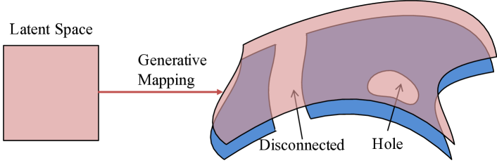
Figure 1: The true underlying structure of the data is generally non-simply-connected (blue), whereas the manifold induced by the deep generative model is simply-connected (red). This topological difference degrades the quality of the interpolation computed on the deep generative model.

Notations

We denote the latent space as $Z$, the input data space as $X$ and the coordinates of each space as $z$ and $x$ respectively. We do not use bold letter for the vectors or matrices, but brackets $[\cdot]$ are used when explicit indication of matrix is needed.

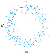
(a)

(b)

(c)

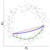
(d)

Figure 2: (a) 2-D circular dataset (b) GAN (2-20-20-2) trained on the dataset. Transformed 2-D latent space grid is shown. Note that the grid also covers the hole in the center due to the topological constraint. (c) $p(x)$ shown in $Z$ coordinates with heat map (i.e., $z\mapsto x\mapsto p(x)$). The central area of the latent space is mapped to the hole in the input space, thus has a low density. (d) Comparison of the interpolation methods– Blue-solid: linear interpolation method found in previous literature; Red-dotted: geodesic interpolation method; Green-dash-dotted: geodesic with density regularizer.

Gradient Descent Method to Compute the Geodesic Interpolation

In this section, we introduce a path-energy loss function and corresponding gradient descent method to compute the geodesic curve between two data points.

As the manifold of deep generative model is defined via the latent space and the generative mapping, curves on the manifold can be parameterized in the latent space. The length is measured using the Riemannian metric $g_{mn}(z)$, which is induced from the Euclidean metric of the ambient data space $X$. The mathematical relationship can be written as $g_{mn}(z)\dot{z}^{m}\dot{z}^{n}=\delta_{kl}\dot{x}^{k}x^{l}$ using Einstein notation and the Kronecker delta, where the details can be found in (?; ?).

Now, let $z(t):[a,b]\to U$ be a curve in a latent space with boundary conditions $z(a)=z_{a}$ and $z(b)=z_{b}$. The length of $z(t)$ under metric $g$ is given as $L(z)=\int_{a}^{b}\|dz/dt\|_{g}dt=\int_{a}^{b}\left(\sqrt{\sum_{m,n}g_{mn}(z)\dot{z}^{m}\dot{z}^{n}}\right)dt$. Instead of directly minimizing the length $L(z)$, minimizing the energy $E(z)=\int_{a}^{b}\epsilon(z)dt=\int_{a}^{b}\left(\frac{1}{2}\sum_{m,n}g_{mn}(z)\dot{z}^{m}\dot{z}^{n}\right)dt$ gives the same result yet in an algebraically simpler form, by noting that $L(z)=2(b-a)E(z)$ if $\|dz/dt\|_{g}=1$. Thus the formulation to obtain the geodesic is reduced to

$$z^{*}=\arg\min_{z}E(z)\quad\text{subject to}\quad\|\dot{z}\|_{g}=1.$$

To minimize the energy $E(z)$, we compute the gradient according to a small change $\zeta$ to the curve $z$ ($\zeta:[a,b]\to Z$ with $\zeta(a)=\zeta(b)=0$). This is given as a Gâteaux derivative: $\delta E(z;\zeta)=\int_{a}^{b}\left(\frac{\partial\epsilon}{\partial z}-\frac{d}{dt}\frac{\partial\epsilon}{\partial\dot{z}}\right)\zeta dt$, which is the functional analogue of directional derivative.

Note that the Euler-Lagrange equation is derived in a process of finding $\delta E(z;\zeta)=0$ regardless of $\zeta$, but it is intractable to solve since the metric $g$ described by neural network is too complicated. We instead seek the steepest gradient change $\zeta^{*}=\arg\max_{\zeta}\delta E(z;\zeta)$, which is derived using the Cauchy-Schwarz inequality,

$$\zeta_{i}^{*} =\frac{\partial\epsilon}{\partial z^{i}}-\frac{d}{dt}\frac{\partial\epsilon}{\partial\dot{z}^{i}}=-\sum_{k}g_{ik}(\ddot{z}^{k}+\sum_{m,n}\Gamma_{mn}^{k}\dot{z}^{m}\dot{z}^{n}),$$

where $\Gamma_{nm}^{k}=\frac{1}{2}g^{kl}\left(\partial g_{kn}/\partial z^{m}+\partial g_{mk}/\partial z^{n}-\partial g_{mn}/\partial z^{k}\right)$ is the Christoffel Symbol. Note that $\Gamma_{nm}^{k}$ is purely related to the local change of the coordinate bases, thus it becomes zero in the input-space coordinates. Also, the metric is described as Kronecker delta in input-space coordinates, so the equation is far simplified as

$$\xi_{i}^{*}=-\ddot{x}_{i},$$

where $\xi$ is a small change to the curve $x$ described in the input-space coordinates.

To summarize, for a curve $z(t)$ in $U\subset Z$, we transform every point on the curve to the input space using the generative mapping, from which the corresponding curve $x(t)$ in $M\subset X$ is obtained. Then, we compute the acceleration $\ddot{x}$ to get the steepest gradient descent change toward minimizing the path-length of the curve. By iteratively updating $x\leftarrow x+\eta\ddot{x}$ ($\eta$ is a learning rate), $x$ will converge to the shortest path. Finally, putting $x$ back to the latent space will give the geodesic in the latent space. More detailed algorithm can be found in (?) and the extended version with our proposing regularizer will be described in the next section.

Density Regularizer

As introduced earlier, the topological difference between the deep generative model and the dataset brings a serious problem in the interpolation. For example, consider a circular dataset and the geodesic between two points in the dataset (Fig. 3). It is natural to think that the geodesic should follow a circular path between two points and pass through dense regions. However, as the hole in the center is a valid region for deep generative models, the geodesic becomes a linear path and passes through the hole (Red-dotted curve in Fig. 3 (d)).

In order to prevent the geodesic from finding this kind of shortcuts, we propose to add a density regularizer term to the energy functional:

$$\mathcal{L}(z;\mu) =E(z)+\mu\int_{a}^{b}\left(-\log p(z)+\frac{1}{2}\log\left|\det[g_{z}]\right|\right)dt,$$

where $\mu>0$ is a regularization weight. The regularization term is in fact an integrated negative log-probability-density $-\log p(x)$ along the curve, thus it keeps the curve from passing through low-density regions.

In Fig. 3 (c) it can be seen that the density $p(x(z))$ is low in the central area of the latent-space, which is mapped to the hole of the input data space. Introduction of the regularizer results in an interpolation avoiding this low-density regions, while keeping its path-length as short as possible (Green-dash-dotted curve in Fig. 3 (d)).

Numerical Algorithm for Geodesic Interpolation

As explained in the previous section, geodesic curve can be computed by iteratively updating every point on the curve $z(t)$ toward the steepest variational direction $\zeta^{*}$. In practice, we approximate the curve with a set of points $z^{k}$. As for $\zeta^{*}$, we first compute $\xi^{*}=-\ddot{x}$ using finite difference method, then pull back the vectors $\xi^{*}$ to the latent space using the pseudo-inverse of the Jacobian matrix. The contribution from the gradient of the density regularizer is added to the obtained $\zeta^{*}$.

Initial ordered sequence $z^{k}$

Compute $x^{k}=f(z^{k})$, $J^{k}=J(z^{k})$ for $k=1,\cdots,K$

while not converged do

     $v^{k}\leftarrow\frac{x^{k+1}-x^{k}}{\|x^{k+1}-x^{k}\|}$     for $k=1,\cdots,K-1$

     $a^{k}\leftarrow v^{k}-v^{k-1}$     for $k=2,\cdots,K-1$

     $b^{k}\leftarrow({J^{k}}^{\top}J^{k})^{-1}{J^{k}}^{\top}a^{k}$  for $k=2,\cdots,K-1$

     $z^{k}\leftarrow z^{k}+\eta\left(b^{k}-\mu\frac{\partial}{\partial z}\left(\frac{1}{2}\log\det([g])-\log p(z)\right)\rvert_{z=z^{k}}\right)$

         for $k=2,\cdots,K-1$

     Compute $x^{k}$, $J(z^{k})$ for $k=1,\cdots,K$

end while

Algorithm 1 Geometric Interpolation with Density Regularizer

Experiments

Datasets, Models and Hyperparameters

In experiments, we use two different image datasets: 1) MNIST (?), and 2) Yale (?). Yale dataset originally consists of face images of 28 individuals, but only a single person images (under 64 different illumination conditions) are used to examine the illumination manifold.

We use three different deep generative models, where each of which is paired with the datasets. 1) MNIST with GAN (?), 2) MNIST with VAE (?), 3) Yale with DCGAN (Deep Convolutional GAN) (?).

When running the numerical algorithm to compute the geodesic, number of approximation points is fixed to 35. We observed that too large number of approximation points sometimes yield an entire break-up of the smoothness of the curve due to the approximation noise. Regularizer weight $\mu$ is empirically determined, ranging from 0.1 ~ 0.003 according to each setting.

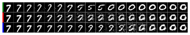
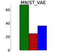
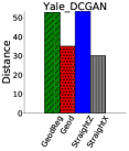
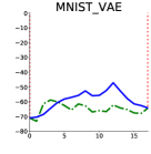
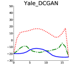
Figure 3: Interpolation results from MNIST GAN, MNIST VAE and Yale DCGAN models, using different methods. In all plots, colors are matched according to the interpolation methods: Geodesic with Density Regularizer (green), Geodesic (red), Straight in $Z$ (blue). Aside from the colors, the images are organized in order of GeodReg, Geod, StraightZ, from top to bottom. Corresponding distances are shown in the left with striped, dotted, plain bar graphs. Negative Log-Likelihood along the interpolation points on the path are shown at the bottom with dash-dotted, dotted, plain curves.

Interpolations and the Effect of the Regularizer

In Fig. 3, we show the results from geodesic interpolation method, with and without the density regularizer, as well as the results from a naïve method that follow a straight line in $Z$. Hereafter, we denote each method as GeodReg, Geod and StraightZ respectively.

In MNIST results, it can be clearly seen that GeodReg outperforms others in terms of quality. GeodReg shows smooth transitions along realistic samples, whereas Geod and StraightZ contain some mottled, non-number-like images. Geod and StraightZ do not consider the probability density, thus cannot avoid low density regions as shown in the log-density plot in the bottom. Geod particularly passes through much lower density regions, but instead has the shortest length among others. Note that these results agree with the toy example shown in Fig. 3 (d).

Lambertian Image Manifold

According to (?), object images taken under various illumination conditions form a 9-D linear manifold if the object has Lambertian reflectance. Yale face dataset matches up to the Lambertian condition in practice (?), thus we examine if our interpolation methods find linear paths on Yale dataset.

In the left pane of the Fig. 4, it can be seen that the length obtained from Geod is shortest thus closest to the true length. In the right pane, it can be seen that the path found by Geod is the straightest in the input space, as it has the smallest cosine dissimilarity to the true linear path. GeodReg deviates from the true path while seeking high density but still close to it compared to StraightZ as seen from the right pane.

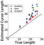
Figure 4: Results from Yale dataset. (Left) Lengths of the curves obtained from different interpolation methods, compared to the ground truth length. (Right) Cosine dissimilarities between the tangent vectors at each point on the curve and the direction of the true linear path are shown. In both subfigures, Geod finds the shortest and the straightest one, thus closest to the ground truth. Interpolations for 13 different sample pairs are shown.

Concluding Remarks

In this paper, we have proposed a density-regularized geometric interpolation method for deep generative models trained from non-simply-connected datasets. The density regularizer has played a crucial role to compensate the topological difference between the model and the data. Our method has shown superior interpolation qualities over previous linear and geodesic interpolation methods.

References

- [2003] Basri, R., and Jacobs, D. W. 2003. Lambertian reflectance and linear subspaces. IEEE transactions on pattern analysis and machine intelligence 25(2):218–233.
- [1997] Belhumeur, P. N.; Hespanha, J. P.; and Kriegman, D. J. 1997. Eigenfaces vs. fisherfaces: Recognition using class specific linear projection. IEEE Transactions on pattern analysis and machine intelligence 19(7):711–720.
- [2018] Chen, N.; Klushyn, A.; Kurle, R.; Jiang, X.; Bayer, J.; and Smagt, P. 2018. Metrics for deep generative models. In International Conference on Artificial Intelligence and Statistics, 1540–1550.
- [2014] Goodfellow, I.; Pouget-Abadie, J.; Mirza, M.; Xu, B.; Warde-Farley, D.; Ozair, S.; Courville, A.; and Bengio, Y. 2014. Generative adversarial nets. In Advances in neural information processing systems, 2672–2680.
- [2013] Kingma, D. P., and Welling, M. 2013. Auto-encoding variational bayes. arXiv preprint arXiv:1312.6114.
- [1998] LeCun, Y.; Bottou, L.; Bengio, Y.; and Haffner, P. 1998. Gradient-based learning applied to document recognition. Proceedings of the IEEE 86(11):2278–2324.
- [2005] Lee, K.-C.; Ho, J.; and Kriegman, D. J. 2005. Acquiring linear subspaces for face recognition under variable lighting. IEEE Transactions on pattern analysis and machine intelligence 27(5):684–698.
- [2015] Radford, A.; Metz, L.; and Chintala, S. 2015. Unsupervised representation learning with deep convolutional generative adversarial networks. arXiv preprint arXiv:1511.06434.
- [2017] Shao, H.; Kumar, A.; and Fletcher, P. T. 2017. The riemannian geometry of deep generative models. arXiv preprint arXiv:1711.08014.
- [2000] Tenenbaum, J. B.; De Silva, V.; and Langford, J. C. 2000. A global geometric framework for nonlinear dimensionality reduction. science 290(5500):2319–2323.