Causal Mediation Analysis Leveraging Multiple Types of Summary Statistics Data

Abstract

Summary statistics of genome-wide association studies (GWAS) teach causal relationship between millions of genetic markers and tens and thousands of phenotypes. However, underlying biological mechanisms are yet to be elucidated. We can achieve necessary interpretation of GWAS in a causal mediation framework, looking to establish a sparse set of mediators between genetic and downstream variables, but there are several challenges. Unlike existing methods rely on strong and unrealistic assumptions, we tackle practical challenges within a principled summary-based causal inference framework. We analyzed the proposed methods in extensive simulations generated from real-world genetic data. We demonstrated only our approach can accurately redeem causal genes, even without knowing actual individual-level data, despite the presence of competing non-causal trails.

I Introduction

Genome-wide association studies (GWAS) identify statistically significant correlations between genetic and phenotypic variables. In the era of Biobank GWAS, phenotypes can be virtually any variables measurable across millions of individuals in the database, of which examples include diagnosis codes, routine laboratory test results, family history of complex disorders, and even socio-economical status.

Significant signals of well-executed GWAS implicate unidirectional causal relationship from the tagged genomic variants to phenotypes, not the other way. In biological information cascade, using GWAS, we can establish links between the very first (genetics) and the last (phenotypes) layers, and we normally expect the effect sizes are typically minuscule; and necessary statistical significance can be achieved in studies involving at least hundreds of thousands of individuals. Nonetheless, a large number of GWAS summary statistics data are already made publicly available. Geneticists have already uncovered more than 24k unique associations between single nucleotide polymorphism (SNP) markers and complex phenotypes MacArthur et al. (2017).

However, a fundamental limitation of GWAS remains in its lack of interpretability. As it can only suggest positions (SNPs) in the human genome without providing any mechanistic insights into how these loci exert their action. Unlike conventional differential gene expression analysis, nearly 90% of significant genetic loci fall non-coding regions Edwards et al. (2013); therefore, even knowing a target gene and relevant regulatory context is already a big challenge in most post-GWAS analysis. Obviously, by characterization of gene names and related pathways beyond a set of genomic locations, we can begin to understand biological mechanisms to find a suitable entry point of therapeutics.

We recognize interpretation of GWAS can be improved by solving a series of causal mediation problems. The basic idea is to jointly analyze GWAS data with other types of genetic association statistics that connect genetic variants (SNPs) to endo-phenotypes located in the middle between genetic and phenotypic layers. We transfer knowledge of intermediate genetic regulatory mechanisms to marginalized GWAS summary data Claussnitzer et al. (2015).

$$\textrm{GWAS:}\quad\textsf{SNP}\to \overbrace{\cdots}^{\textrm{unknown}} \to\textsf{disease}$$

$$\textrm{eQTL:}\quad\textsf{SNP}\to$$ gene

$$\textrm{mediation:}\quad\textsf{SNP}\to \to\textsf{disease}$$ gene

Of many possible types of endo-phenotypes, we focus on finding a set of causal genes that mediate between initiating SNPs and target phenotypes, such as complex diseases. We leverage the knowledge of existing eQTL (expression qualitative trait locus) summary statistics. In eQTL summary statistics data, we compile effect sizes of genetic associations of nearly 20k genes with common genetic variants (SNPs). On each gene, approximately 1k-10k neighboring SNPs are typically tested within a $\pm$ 1 megabase window (cis-eQTLs). Since we only investigate mediation of cis-regulatory mechanisms, mediation analysis can be conducted within a segment of genome. We break down the whole genome into 1,703 independent blocks Berisa & Pickrell (2016).

In “causal” mediation analysis, we emphasize that correlation is never causality because observed gene-disease association / correlation signals can be interpreted as many different causal mechanisms (Fig.1). Of them, we are particularly interesting in redeeming the mediation effect; only the mediating gene can causally alter predisposition of the disease.

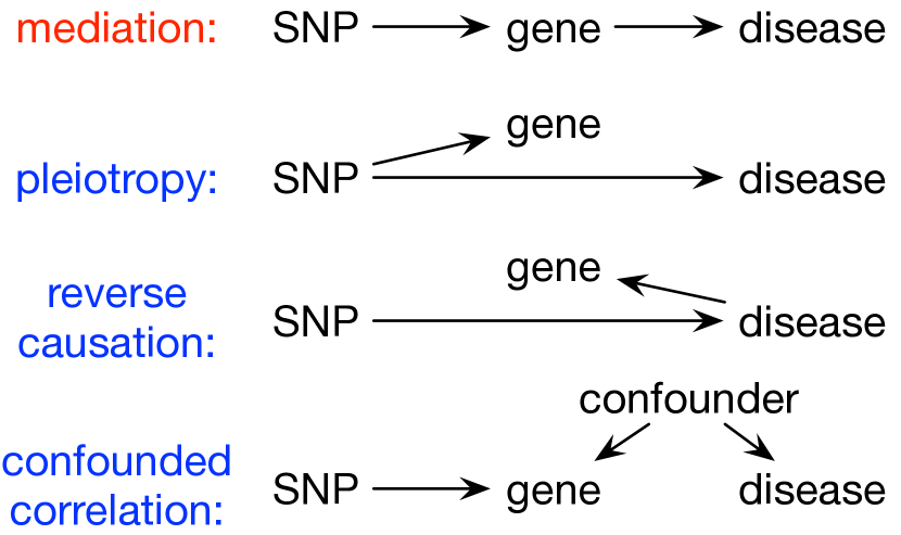
Figure 1: Association between gene and disease can be interpreted in multiple ways.

Our contributions

In this work, we contribute a general causal inference method for multivariate mediation analysis, leveraging two types of summary statistics data–one linking instrumental variables (genetics) to outcome variables (phenotypes) and the other linking instrumental variables with mediator variables (endo-phenotypes; genes).

First, we carefully examine the underlying mediation problem in details, and reveal that a subtle difference can substantially alter identifiability of the underlying statistical problem. We claim that practical issues, such as incomplete knowledge of mediation, polygenic bias, and uncharacterized confounding effects, should be carefully controlled; otherwise, association-based methods may pile up wrong interpretation of GWAS results.

Second, to our knowledge, this work is the first attempt in summary-based mediation analysis to include and test multiple mediation variables within a single Bayesian framework. Our formalism might be summary-based translation of the existing proposal for fully observed individual-level data VanderWeele & Vansteelandt (2014), but we address practical issues hidden underneath the observed summary statistics.

Third, our approach is built on a principled multivariate model, which takes into accounts of inherent dependency structure between a large number of genetic variants. We resolve the unavoidable issue of high-dimensional collinearity using sparse Bayesian variable selection Mitchell & Beauchamp (1988), and demonstrate that our Bayesian approach yields superior performance in relevant simulations.

Fourth, we propose novel, yet simple, operational steps generally applicable to summary-based causal inference problems. We solve a long-standing problem of confounder correction in genetics data, not relying on unrealistic simplifications and assumptions.

Related work

Mendelian Randomization (MR) Smith & Ebrahim (2004); Katan (2004) resolves causal directions by using genetic variants as instrumental variables (IV) in causal inference analysis. However, MR assumes that entire proportion of causal effects in the genetic locus on the phenotype are mediated by the measured intermediate phenotype (e.g. expression of a given gene in the given cell type) Smith & Ebrahim (2004); Davey Smith & Hemani (2014), which asserts there is no other causal trails exist, and more importantly most MR method only works on a few IV variants.

Transcriptome-wide association studies (TWAS) aggregates information of multiple variants to find genes whose regulatory variants have correlated effect sizes for both gene expression and downstream phenotypes Gamazon et al. (2015); Gusev et al. (2016); Mancuso et al. (2017). However, TWAS methods are fundamentally limited because they cannot distinguish between causal mediation, pleiotropy, linkage between causal variants, and reverse causation, which could lead to inflated false positives.

II Causal mediation analysis

II.1 A generative model of phenotypic variability mediated by gene expressions

We model a phenotype vector $\mathbf{y}$ of $n$ individuals as a function of genotype information measured across $p$ common variants (SNPs).

$$\mathbf{y}\sim X\boldsymbol{\theta}+\boldsymbol{\epsilon},\quad\boldsymbol{\epsilon}\sim\mathcal{N}\!\left(\mathbf{0},\sigma^{2}I\right)$$ (1)

with the multivariate effect size $\boldsymbol{\theta}$. We assume irreducible isotropic noise $\epsilon$ fluctuates with some variance $\sigma^{2}$. For simplicity, we assume the GWAS trait is quantitative, $y_{i}\in\mathbb{R}$ and the genotype matrix $X$ is column-wise standardized with mean zero and unit standard deviation.

Conventional definition of GWAS statistics refers a univariate effect size (a regression slope of a simple regression (or log-odds ratio) in case-control studies) measured on each genetic variant. In summary data, we have a vector of $p$ summary statistics, effect size $\hat{\theta}_{j}$ and corresponding variance $\hat{\sigma}^{2}_{j}$ for each SNP $j\in[p]$.

$$\hat{\theta}_{j}=\frac{\mathbf{x}_{j}^{\top}\mathbf{y}}{\mathbf{x}_{j}^{\top}\mathbf{x}_{j}}\quad\textrm{and}\quad\hat{\sigma}_{j}^{2}=\frac{(\mathbf{y}-\mathbf{x}_{j}\hat{\theta}_{j})^{\top}(\mathbf{y}-\mathbf{x}_{j}\hat{\theta}_{j})}{n\mathbf{x}_{j}^{\top}\mathbf{x}_{j}}.$$ (2)

However, due to linkage disequilibrium (LD; correlations between neighboring SNPs), an effect size measured on each single variant contains contributions from the neighboring SNPs.

Likewise, expression profiles of $K$ genes are generated by the same type of models on the shared genotype matrix $X$. For each gene $k\in[K]$, we define a generative model of gene expression $\mathbf{m}_{k}$:

$$\mathbf{m}_{k}=X\boldsymbol{\alpha}_{k}+\boldsymbol{\delta}_{k},\quad\boldsymbol{\delta}_{k}\sim\mathcal{N}\!\left(\mathbf{0},\tau_{k}^{2}I\right)$$ (3)

where multivariate eQTL effect size vector $\boldsymbol{\alpha}_{k}$ exerts an action on each gene $k$, but there is a measurement error $\delta$ with non-genetic variance $\tau_{k}$.

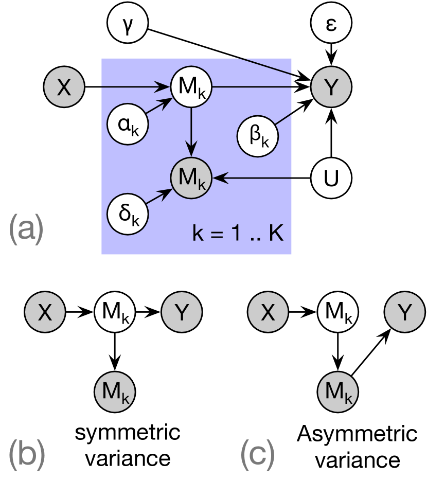
Figure 2: (a) A graphical model for the full generative scheme with $K$ genes. $X$: genotype matrix; $M$ (unfilled): genuine mediation effect; $M$ (filled): observed mediation variable; $Y$: phenotype measurement; $U$: unmeasured confounding variable; $\alpha$: eQTL effect size; $\beta$: mediation effect size; $\gamma$: unmediated effect size; $\delta$: non-genetic components in gene expression variation; $\epsilon$: non-genetic components in phenotypic variation. (b) The symmetric variance model (see the text). (c) The asymmetric variance model (see the text).

II.2 Two types of mediation models

Before we present methods and algorithms, we digress to dissect identifiability issues with intuitive examples.

Total genetic effect $X\boldsymbol{\theta}$ on the phenotypic variation (Eq.1) decomposes into two components, mediated from the causal genes $X\boldsymbol{\alpha}_{k}\beta_{k}$ with mediation effect size $\beta_{k}$ and unmediated effects $X\boldsymbol{\gamma}$ with some coefficients $\boldsymbol{\gamma}$. In other words, $X\boldsymbol{\theta}=X(\sum_{k}\boldsymbol{\alpha}_{k}\beta_{k}+\boldsymbol{\gamma})$.

Overall, this generative scheme (Fig.2a) is generally acceptable to most of genetics and epidemiology research community, but we demonstrate a subtle, yet critical difference about when we actually measure the mediation profiles with non-genetic stochasticity $\delta$ (Fig.2b versus c) can make impact on identifiability. In the former model (b), we assume that the non-genetic components $\delta$ are mostly attributable to technical covariates, and estimable through control genes in eQTL analysis Gagnon-Bartsch & Speed (2012); Risso et al. (2014), whereas in the latter case (c), non-genetic signals $\delta$ first biologically incorporate and become transmitted to downstream phenotypic variation. We term them symmetric and asymmetric variance models, respectively, as they result in different variance structures in the following model identification steps.

Symmetric variance model

For intuitive explanation, without loss of generality, suppose we only have a single gene and a single genetic variant in the model. If we assume stochasticity was infused after the mediation, we generate the phenotype by

$$\mathbf{y}=\mathbf{x}\alpha\beta+\mathbf{x}\gamma+\boldsymbol{\epsilon},$$

but we only observe gene expression with stochasticity, $\mathbf{m}=\mathbf{x}\alpha+\boldsymbol{\delta}$ with $\boldsymbol{\delta}\sim\mathcal{N}\!\left(\mathbf{0},\tau^{2}I\right)$. However, we can obtain unbiased estimation of the eQTL effect, $\boldsymbol{\mu}\equiv\mathbf{x}\alpha$, and use this to test the mediation of this gene expression.

We set up two regression problems: (1) $\mathbf{y}\sim\boldsymbol{\mu}\beta$ (for the mediated effect) and (2) $\mathbf{y}\sim\mathbf{x}\theta$ (for the direct / unmediated effect). Straightforward algebraic derivation characterize the distribution of estimate $\hat{\beta}$ as

$$\hat{\beta} \sim \mathcal{N}\!\left(\beta+\alpha^{-1}\gamma,\sigma^{2}n^{-1}\alpha^{-2}\right),$$

and the estimated mediated effect size follows

$$\hat{\alpha}\hat{\beta}\sim\mathcal{N}\!\left(\alpha\beta+\gamma,\frac{\sigma^{2}}{n}\right).$$

This coincides with the same distribution of direct (marginal) GWAS statistic:

$$\hat{\theta}=\frac{\mathbf{x}^{\top}\mathbf{y}}{\mathbf{x}^{\top}\mathbf{x}}\sim\mathcal{N}\!\left(\alpha\beta+\gamma,\frac{\sigma^{2}}{n}\right).$$

Remark: Not only we have the same mean, but also the variance in both causal trails is symmetric. Two causal trails are non-identifiable Gusev et al. (2016); Barfield et al. (2018), unless we apply a suitable causal inference method.

Asymmetric variance model

However, if we assume stochasticity was infused before the mediation, we generate the phenotype by

$$\mathbf{y}=(\mathbf{x}\alpha+\boldsymbol{\delta})\beta+\mathbf{x}\gamma+\boldsymbol{\epsilon},$$

and it yields asymmetric variance models. The effect size distribution of the estimated mediated trail follows

$$\hat{\alpha}\hat{\beta}\sim\mathcal{N}\!\left(\alpha\beta+\gamma,\frac{\beta^{2}\tau^{2}+\sigma^{2}}{n}\right)$$

since the gene-level association effect size follows

$$\hat{\beta} \sim \mathcal{N}\!\left(\beta+\alpha^{-1}\gamma,(\beta^{2}\tau^{2}+\sigma^{2})n^{-1}\alpha^{-2}\right).$$

On the other hand, direct genetic association statistic takes a rather different form of distribution:

$$\hat{\theta} = \frac{\mathbf{x}^{\top}\mathbf{y}}{\mathbf{x}^{\top}\mathbf{x}}\sim\mathcal{N}\!\left(\alpha\beta+\gamma,\frac{\tau^{2}+\sigma^{2}}{n}\right).$$

Remark: These two distributions are distinguishable by the asymmetry of variance. Whenever there is non-zero mediation effects, $\beta\neq{0}$, we will have larger fluctuation of the mediated effect, but in standard error estimation we will omit $\beta^{2}\tau^{2}/n$ and under-estimate the variance as $\sigma^{2}/n$. Moreover, if gene expression heritability is lower, meaning higher $\tau^{2}$, the identification problem becomes easier. This is somewhat paradoxical.

MR community Bowden et al. (2015); Hartwig et al. (2017) has adopted this type of generative models in their simulation studies, but it appears that we may not need strong causal assumptions to identify mediation effects under this type of model since we can identify causal effects by brute-force model estimation.

II.3 Practical issues in mediation analysis

Strongest correlation is not necessarily causation

First of all, we assume true data generation scheme is much closer to the symmetric variance model than the asymmetric variance model. Although we have investigated the asymmetric variance assumption and our method excels, we concluded that performance under the asymmetric model largely depends on statistical estimation accuracy, rather than causal inference.

Missing mediation problem

All genes are heritable by definition, but only some of them are measurable in given eQTL data. It may stem from the lack of statistical power, or true genetic variation of expression profiles may be conditional with respect to a certain cellular context. Moreover, it is not difficult to imagine that a causal gene can be included in the missing component of mediation effect. In that case, another non-causal gene correlated with the causal one can easily lead to a false conclusion.

Pleiotropic and polygenic bias

The missing mediation problem can be exacerbated when there is substantial amount of unmediated genetic, thus independently pleiotropic, effect on the phenotype within LD (the second one in Fig.1). It is commonly observed that this pleiotropic effect is also highly polygenic, and creates lots of confusions in causal mediation analysis.

III Causal inference on summary statistics

A generative model of GWAS summary statistics

For simplicity, letting $S_{jj}=\hat{\sigma}_{j}^{2}+\hat{\theta}^{2}/n$, we can redefine a model equivalent to the previous one (Eq.1) with respect to $p$-dimensional summary statistics, the regression with summary statistics (RSS) model (Zhu & Stephens, 2017):

$$\hat{\boldsymbol{\theta}}\sim\mathcal{N}(SRS^{-1}\boldsymbol{\theta},SRS).$$ (4)

Normally we have large enough sample size ($n\to\infty$), the RSS model resorts to a fine-mapping model (Hormozdiari et al., 2014). Generative scheme of a GWAS z-score vector, with each element $z_{j}=\hat{\theta}_{j}/\hat{\sigma}_{j}$, is described by the reference LD matrix $R$ and true (multivariate) effect size vector $\theta$.

$$\mathbf{z}\sim\mathcal{N}(R\boldsymbol{\theta},\sigma^{2}R).$$ (5)

Reparameterized stochastic variational inference

The key challenge in fitting the RSS model is dealing with the covariance matrix in the likelihood. To address this challenge, we exploit the spectral decomposition of the LD matrix Lippert et al. (2011). With a singular value decomposition (SVD) of the genotype matrix, such as

$$(n)^{-1/2}X=UDV^{\top},$$ (6)

we deal with the LD matrix $R=VD^{2}V^{\top}$ and redefine a new design matrix ${\tilde{X}\equiv V^{\top}}$ and a transformed outcome vector ${\tilde{y}_{t}\equiv V^{\top}S^{-1}\hat{\boldsymbol{\theta}}_{t}}$ to obtain equivalent, but fully factorized, multivariate Gaussian model:

$$y_{t}\sim\mathcal{N}\!\left(D^{2}\tilde{X}S^{-1}\boldsymbol{\theta}_{t},D^{2}\right).$$

Further, letting ${\eta_{k}\equiv\sum_{j=1}^{p}V_{jk}S_{j}^{-1}\theta_{j}}$, we can rewrite the transformed log-likelihood of the model for each eigen component $i$:

$$\ln P(\tilde{y}_{i}|\eta_{i})=-\frac{1}{2}\ln d_{i}^{2}-\frac{1}{2d_{i}^{2}}(\tilde{y}_{i}-d_{i}^{2}\eta_{i})^{2}-\frac{1}{2}\ln(2\pi).$$

We carry out stochastic variational inference Paisley et al. (2012) by simulating stochasticity of $\eta$ by simple reparameterization Kingma et al. (2015) in the space of eigen vectors, not on the space of SNPs in higher-dimensional space.

Derivation of summary-based mediation model

We present the full description of generative model,

$$\mathbf{y}\sim\mathcal{N}\!\left(\sum_{k\in[K]}X\boldsymbol{\alpha}_{k}\beta_{k}+X\boldsymbol{\gamma},\sigma^{2}I\right),$$

where the products of eQTL and mediation coefficients, $\boldsymbol{\alpha}_{k}\beta_{k}$, capture mediation effects and $\boldsymbol{\gamma}$ denotes multivariate effect sizes of the unmediated / direct pathway. We can reformulate an equivalent model in terms of summary z-scores:

$$\mathbf{z}^{\textsf{gwas}} \approx (\sigma^{2}n)^{-1/2}X^{\top}\mathbf{y}$$

$$\sim \mathcal{N}\!\left(\frac{\sqrt{n}}{\sigma}R\sum_{k}\boldsymbol{\alpha}_{k}\beta_{k}+\frac{\sqrt{n}}{\sigma}R\boldsymbol{\gamma},R\right).$$

Likewise, we can characterize distribution of each gene $k$’s univariate z-score vector as:

$$\mathbf{z}^{\textsf{eQTL}}_{k} \approx n^{-1/2}X^{\top}\mathbf{m}_{k}$$

$$\sim \mathcal{N}\!\left(n^{-1/2}R\boldsymbol{\alpha}_{k},\tau^{2}R\right).$$

Assuming that we tightly controlled measurement errors in the eQTL data, i.e., $\tau^{2}\to 0$, we can substitute the terms on the mediation effects of the GWAS model with the z-scores of eQTL effects:

$$\mathbf{z}^{\textsf{gwas}} \sim \mathcal{N}\!\left(\sum_{k\in[K]}\mathbf{z}^{\textsf{eQTL}}_{k}\beta_{k}+n^{-1/2}R\boldsymbol{\gamma},R\right).$$ (7)

Identification of the unmediated “pleiotropic” effects

Causality of this multivariate model can be made by statistical inference as long as the unmediated effect $\boldsymbol{\gamma}$ is estimable. To make it identifiable, previous methods Barfield et al. (2018); Bowden et al. (2015) reduce the degree of freedom in the $\boldsymbol{\gamma}$ parameters down to a mere intercept term. However, our simulation suggests that sheer Bayesian inference on the full multivariate $\boldsymbol{\gamma}$ is indeed estimable if the GWAS and eQTL summary statistics were generated by the asymmetric variance model.

On the other hand, in the symmetric variance model, naive inference algorithm yields poor performance since all the genuine mediation effects will be included in the unmediated effect. We need to include an additional step to construct features to characterize overall contribution of the unmediated causal trails $X\boldsymbol{\gamma}$.

We first characterize independent components of genetic variation across multiple genes and diseases. For one GWAS and $K$ eQTL z-scores, letting,

$$\tilde{Z}\equiv(\mathbf{z}^{\textsf{gwas}},\mathbf{z}_{1}^{\textsf{eQTL}},\ldots,\mathbf{z}_{K}^{\textsf{eQTL}}),$$ (8)

we profile overall spectrum of variation by solving the following sparse factorization problem:

$$\mathbb{E}\left[\tilde{Z}\right]=n^{-1/2}X^{\top}\left(\sum_{l\in\textrm{factors}}\mathbf{c}_{l}\boldsymbol{\omega}_{l}^{\top}\right).$$ (9)

From this result, we obtain covariate matrix $C$, which we can consider as projection of overall genetic variations onto reference panel genotype space. We use this rich vocabulary of $C$ matrix to adjust potential unmediated effects.

However, care should be taken. We exclude any column vector $\mathbf{c}_{l}$ if the corresponding $\boldsymbol{\omega}_{l}$ vector contains strong non-zero elements in both GWAS and eQTL sides. For instance, we call the $l$-th column is associated with gene (or trait) $k$ if posterior inclusion probability of $\omega_{kl}$ greater than 1/2. Our decision rule is largely compatible with the widely accepted InSIDE (instrument strength independent of direct effect) condition Bowden et al. (2015), but we actively search for independent unmediated effects. On the selected $L$ unmediated effects $\mathbf{c}_{l}$, $l\in[L]$, we can easily construct z-scores, $\mathbf{z}_{l}^{\textsf{unmed}}=n^{-1/2}X^{\top}\mathbf{c}_{l}$, we then resolve mediated and unmediated effects in the following joint model:

$$\mathbf{z}^{\textsf{gwas}}\sim\mathcal{N}\!\left(\sum_{k\in[K]}\mathbf{z}_{k}^{\textsf{eQTL}}\beta_{k}+\sum_{l\in[L]}\mathbf{z}_{l}^{\textsf{unmed}}\gamma_{l},R\right),$$ (10)

where both $\beta$ and $\gamma$ follow the spike-slab prior Mitchell & Beauchamp (1988).

Identification of hidden non-genetic confounding effects

The sparse factorization result (Eq.9) still provides a valuable resource in checking spurious correlations confounded by non-genetic factors (the third and fourth in Fig1). However, there is a risk of over-correcting genuine genetic correlations at the same time. We can sidestep such a possibility by constructing a proxy data matrix $\tilde{Z}^{(0)}$, on which we can warrant orthogonality with a genotype matrix. The idea is that we project our z-score matrix $\tilde{Z}$ (Eq.8) onto independent LD blocks to adaptively construct the proxy matrix for factorization analysis.

More precisely, we define non-genetic confounding effect $\mathbf{u}$ between a gene expression $\mathbf{m}$ and phenotype vector $\mathbf{y}$ as follows.

$$\mathbf{m} = X\boldsymbol{\alpha}+\mathbf{u}+\boldsymbol{\delta}$$

$$\mathbf{y} = X\boldsymbol{\alpha}\beta+X\boldsymbol{\gamma}+\mathbf{u}+\boldsymbol{\epsilon}.$$

Even though we have $\mathbb{E}\!\left[\mathbf{u}^{\top}(X\boldsymbol{\alpha})\right]=0$ by definition, gene-level correlation would have risk of including non-causal effects:

$$\mathbf{m}^{\top}\mathbf{y}=\underbrace{(\boldsymbol{\alpha}^{\top}X^{\top}X\boldsymbol{\alpha})\beta}_{\textrm{causal}}+\underbrace{\mathbf{u}^{\top}(X\boldsymbol{\gamma})+\mathbf{u}^{\top}\mathbf{u}}_{\textrm{non-causal correlation}},$$

where we may expect the second term to vanish with large $n$, but the third term persists.

We propose a simple operator to make intervention only on the putative genetic components to yield a valid proxy z-score matrix can selectively capture non-genetic confounding effects.

As human LD patterns are close to a block-diagonal covariance matrix, we can always find an independent LD block $X^{(0)}$ such that for all columns $j$ of $X^{(0)}$ is orthogonal to the mediation effect, i.e., $\mathbb{E}\!\left[(X^{(0)}_{j})^{\top}(X\boldsymbol{\alpha})\right]=0$. Before we carry out the factorization (Eq.9), we project the combined z-score matrix of $X$ onto some independent LD block $X^{(0)}$:

$$\tilde{Z}^{(0)}\leftarrow(X^{(0)})^{\top}(X^{-\top}\tilde{Z}).$$ (11)

As for the inverse step, we consider pseudo-inverse; by SVD (Eq.6), $X^{-\top}=UD^{-1}V^{\top}$. We perform factorization on this $\tilde{Z}^{(0)}$,

$$\mathbb{E}\!\left[\tilde{Z}^{(0)}\right]=n^{-1/2}(X^{(0)})^{\top}C\Omega$$ (12)

and use $n^{-1/2}X^{\top}C$ to account for non-genetic correlations.

Remark: We can justify this can effectively eliminate genetic effects from summary statistics: Provided that linear transformation of multivariate Gaussian distribution yields Gaussian distribution, we characterize the mean vector and the covariance matrix after each step of transformation. Without loss of generality, underlying $n$ individual-level target vector $\mathbf{y}$ has two components, $X\boldsymbol{\alpha}$ and $\mathbf{u}$. This induces the distribution of z-score vector: $\mathbf{z}\sim\mathcal{N}\!\left(n^{-1/2}X^{\top}(X\boldsymbol{\alpha}+\mathbf{u}),n^{-1}X^{\top}X\right)$. After the first transformation, we have

$$X^{-\top}\mathbf{z}\sim\mathcal{N}\!\left(n^{-1/2}X\boldsymbol{\alpha}+n^{-1/2}\mathbf{u},n^{-1}I\right).$$

Followed by the second transformation, we have

$$X_{0}^{\top}(X^{-\top}\mathbf{z})\sim\mathcal{N}\!\left(n^{-1/2}X_{0}^{\top}\mathbf{u},n^{-1}X_{0}^{\top}X_{0}\right),$$

because $\mathbb{E}\!\left[(\mathbf{x}_{j}^{(0)})^{\top}(X\boldsymbol{\alpha})\right]=0$ for all $j$.

IV Experiments

Simulation based on real-world genotype matrix

To evaluate performance of our methods, we carried out extensive and realistic sets of simulations. Unfortunately, there is no labeled data for causal mediation analysis; the only gold standard would be a controlled experiment. We might consider literature-based assessment, but for systematic comparison, we find simulation is more adequate.

We simulate eQTL and GWAS z-scores on selected LD blocks Berisa & Pickrell (2016) using standardized genotype matrix $X$, sampled from the 1000 genomes reference panel The 1000 Genomes Project Consortium et al. (2015), only including individuals with European ancestry ($n$=502), and restricting on the SNPs with minor allele frequency (MAF) $\geq$ 0.05. This results in the matrix $X$ ($n\times{p}$) with $n=502$ and $p$ = 5k-10k SNPs.

We have repeated our experiments using much larger cohort, such as UK10K (Huang et al., 2015) samples ($n$=6,285), but results were qualitatively identical; for brevity, we only report the results of the 1000 genomes data.

We simulate $K=100$ gene expression vectors $\{\mathbf{m}_{k}:k\in[K]\}$, and one phenotype vector $\mathbf{y}$. For each simulation, we provide the following parameters:

• $X$: a genotype matrix (column-wise standardized).

• $g_{g}^{2}$: proportion of gene expression variability explained by genetics; here, we fixed to 0.3.

• $d$: number of causal eQTL SNPs; variability of each gene is determined by a linear combination of $d$ SNPs.

• $\mathbf{u}$: in addition to genetic and unstructured noise components, we have unknown random effect vector.

• $h_{m}^{2}$: proportion of phenotypic variability explained by genetic effects mediated through causal genes.

• $g_{u}^{2}$: proportion of gene expression variability explained by the random effect $\mathbf{u}$.

• $h_{u}^{2}$: proportion of phenotypic variability explained by the random effect $\mathbf{u}$.

Overall simulation steps proceed as follows.

1. Initially all genes are heritable. For each gene $k\in[K]$, sample eQTL effect size $\alpha_{jk}\sim\mathcal{N}\!\left(0,g_{g}^{2}/d\right)$ for the causal SNP $j$ on this gene $k$, but $\alpha_{jk}=0$ for the others. This easily ensures $\mathbb{V}\!\left[X\boldsymbol{\alpha}_{k}\right]=g_{g}^{2}$. Genetic components of this mediator is simply $\mathbf{m}^{(g)}_{k}\leftarrow X\boldsymbol{\alpha}_{k}$.

2. We follow the asymmetric variance model. Sample mediation effect: $\beta_{k}\sim\mathcal{N}\!\left(0,h_{m}^{2}/m\right)$ for the causal genes, otherwise $\beta_{k}=0$; then propagate the mediated genetic effect to a genetic component of phenotype: $\mathbf{y}^{(g)}\leftarrow\sum_{k}\mathbf{m}^{(g)}_{k}\beta_{k}$.

3. For all gene $k\in[K]$, we introduce structured random effects, $\mathbf{m}^{(u)}_{k}\leftarrow\mathbf{u}\xi_{k}$ where $\xi_{k}\sim\mathcal{N}\!\left(0,1\right)$, and rescale this vector such that $\mathbb{V}\!\left[\mathbf{m}^{(u)}_{k}\right]=g_{u}^{2}$.

4. We do the same on the phenotype, $\mathbf{y}^{(u)}\leftarrow\mathbf{u}\xi_{0}$ where $\xi_{0}\sim\mathcal{N}\!\left(0,1\right)$, and rescale this vector such that $\mathbb{V}\!\left[\mathbf{y}^{(u)}\right]=h_{u}^{2}.$

5. For non-heritable (or missing) gene $k$, we eliminate the genetic component, such as $\mathbf{m}^{(g)}_{k}\sim\mathcal{N}\!\left(\mathbf{0},g_{g}^{2}\right)$. Note that this may include a causal mediation gene.

6. The observed expression vector on each gene $k$ is $\mathbf{m}_{k}\leftarrow\mathbf{m}^{(g)}_{k}+\mathbf{m}^{(u)}_{k}+\boldsymbol{\delta}_{k}$ where $\boldsymbol{\delta}_{k}\sim\mathcal{N}\!\left(\mathbf{0},\tau_{0}^{2}I\right)$ with $\tau_{0}^{2}=1-g_{g}^{2}-g_{u}^{2}$.

7. We also observe the phenotype with the noise components: $\mathbf{y}\leftarrow\mathbf{y}^{(g)}+\mathbf{y}^{(u)}+\boldsymbol{\epsilon}$, where $\boldsymbol{\epsilon}\sim\mathcal{N}\!\left(\mathbf{0},\sigma_{0}^{2}\right)$ with $\sigma_{0}^{2}=1-h_{m}^{2}-h_{u}^{2}$.

Data

For summary statistics-based methods, we only provide these two types of z-scores calculated from the simulated data, $\mathbf{y},\mathbf{m}_{k}$, not knowing the genetic part of data, $\mathbf{y}^{(g)},\mathbf{m}_{k}^{(g)}$.

CaMMEL methods

We term our general methodology CaMMEL (causal multivariate mediation extended by LD) as we test multiple mediation effects simultaneously, exploiting local LD structure. Here, we train the CaMMEL model in three different ways and compared them in the simulation studies:

• CaMMEL-naive: Brute-force variational Bayes inference of the joint model with the multivariate unmediated effect sizes (Eq.7).

• CaMMEL-factorization: A two-step inference algorithm where we first characterize the unmediated (direct) effects $\mathbf{z}^{\textsf{unmed}}$ by fitting the factorization model (Eq.9) and resolve the mediation effects in the joint modeling (Eq.10).

• CaMMEL-projection: Another two-step inference algorithm where we first project the combined z-score matrix onto independent LD blocks (Eq.11), then characterize the unmediated effects $\mathbf{z}^{\textsf{unmed}}$ by fitting the factorization model (Eq.12) to adjust non-genetic / unmediated confounding effects. Here, we adjust the GWAS z-score $\mathbf{z}^{\textsf{gwas}}$ by subtracting out the inferred $\mathbf{z}^{\textsf{unmed}}$ and resolve the mediation effects in the joint modeling only with the mediation terms in Eq.10.

Competing methods

As for the calculation of LD-adjusted inverse-variance weighting (IVW) and summary-based TWAS (sTWAS), we first perform SVD of the reference genotype matrix (Eq.6), and this allows estimation of the LD matrix by $R=VD^{2}V^{\top}$. Since we know $\mathbf{z}\sim\mathcal{N}(R\boldsymbol{\theta},R)$. We rotate the original distribution and define another multivariate Gaussian random variable $\boldsymbol{\eta}\equiv D^{-1}V\mathbf{z}\sim\mathcal{N}(DV^{\top}\boldsymbol{\theta},I)$ for algebraic convenience. Let $\boldsymbol{\eta}^{\textsf{eQTL}}\equiv D^{-1}V\mathbf{z}^{\textsf{eQTL}}$ and $\boldsymbol{\eta}^{\textsf{gwas}}\equiv D^{-1}V\mathbf{z}^{\textsf{gwas}}$.

From these two vectors, we can write sTWAS test statistics Mancuso et al. (2017):

$$T^{\textsf{sTWAS}}=(\boldsymbol{\eta}^{\textsf{eQTL}})^{\top}\boldsymbol{\eta}^{\textsf{gwas}}/\sqrt{(\boldsymbol{\eta}^{\textsf{eQTL}})^{\top}\boldsymbol{\eta}^{\textsf{eQTL}}}.$$

Using mr_ivw implemented in Mendelian Randomization package Yavorska & Burgess (2017), we can estimate IVW test statistics:

$$T^{\textsf{IVW}}={\hat{\beta}}^{\textsf{MLE}}\max\{\hat{\sigma},1\}/\mathsf{se}(\hat{\beta}),$$

where $\hat{\beta}^{\textsf{MLE}},\hat{\sigma}^{2}=\arg\max\mathcal{N}(\boldsymbol{\eta}^{\textsf{gwas}}|\boldsymbol{\eta}^{\textsf{eQTL}}\beta,\sigma^{2}I)$ with estimated standard error $\mathsf{se}(\beta)$. We could easily modify the IVW method with different types of linear models, e.g., including an intercept term in the linear model to account for directional pleiotropy, MR-Egger regression Barfield et al. (2018).

Lastly, we compare performance with the observed TWAS (oTWAS), or differential expression analysis, correlation between the observed phenotype $\mathbf{y}$ and noisy observation of gene expression $\mathbf{m}_{k}$.

IV.1 Experiments with strong polygenic bias and missing causal genes

We carried out benchmark tests to evaluate robustness of causal inference in the presence of strong polygenic bias to the phenotype (Fig.3). We sampled 150 genes (using actual gene locations in each LD block) and varied the variance of polygenic bias ($h_{u}^{2}\in\{.2,.3,.4\}$). Of the 150 genes, we excluded 50% of eQTL genes in the observed statistics, which may or may not include two causal genes. To simulate polygenic bias, we followed a previously suggested simulation scheme Barfield et al. (2018), $\mathbf{u}=X\boldsymbol{\gamma}$ where for each $j\in[p]$ $\gamma_{j}\sim\bar{\gamma}+\mathcal{N}(0,10)$ with randomly sampled direction $\bar{\gamma}\in\{+1,-1\}$. We report area under precision recall curve (AUPRC) as metric as we have much fewer causal genes (3) compared to the non-causal ones (147). To be more exact, we only call prediction on a gene is correct if and only if the gene is causal and the sign of predicted effect size also matches with that of the simulated effect.

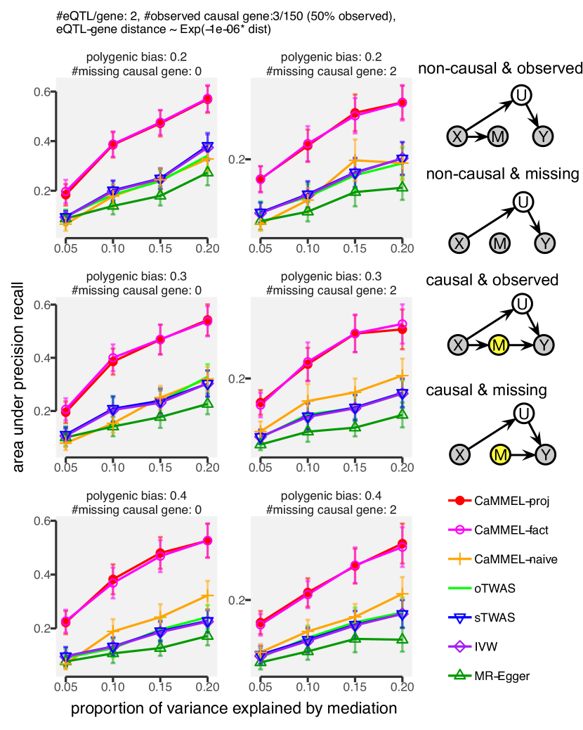
Figure 3: In the experiments under the influence of directional pleiotropy with 50% of genes missing, two of the CaMMEL methods redeem genuine mediation trails with high accuracy.

When there is strong polygenic bias and a substantial fraction of genes are missing, prediction accuracy (and power) of most gene prediction methods can be severely damaged. In human genetics data, unmediated polygenicity is common observed across many different traits, and it is almost impossible for us to obtain a full catalog of eQTL genes. Interestingly, even though we did not include any confounding effect on the mediators (genes), this type of setting is enough to create confusion that univariate (gene-by-gene) methods to make lots of false discoveries. Genes are genetically dependent in LD and become conditionally dependent given phenotype variables. Interestingly, the MR-Egger method has been thought to handle a directional pleiotropy (polygenic bias) Bowden et al. (2015); Barfield et al. (2018), but we could only find the worst performance in our simulations.

On the other hand, when the existing portion of unmediated effects are causally identified, our CaMMEL methods robustly outperform other methods. Yet, naive inference algorithm on the CaMMEL model shows far worse performance because the parameters on the unmediated effect ($\boldsymbol{\gamma}$) are much more adaptable to the data, and yield far too conservative results.

IV.2 Experiments with genes and phenotypes confounded by non-genetic factors

Next, we conducted a new type of benchmark tests where the genes and phenotype are confounded by non-genetic effects. To set apart from the previous experiments, we assumed genes are fully observed for simplicity; by definition, we only considered that the non-genetic confounders are independent of genetics. In most mediation analysis in genetics, we take for granted that such a confounding effect were corrected out by pre-processing steps. However, in practice, especially when there were any sample overlap between eQTL and GWAS cohorts (sharing controls), non-genetic correlations would always exist with a high probability. As we collect more data from biobank (where individuals are totally shared), finding a non-genetic confounder across multiple traits is already a crucial step in GWAS analysis.

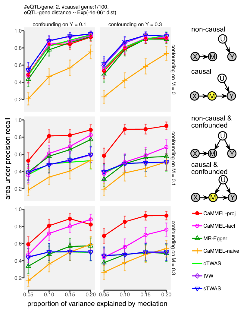
Figure 4: Our method solves a long-standing problem in GWAS: CaMMEL-proj removes non-causal confounding relationships between mediators and outcome variables by projecting correlation structure onto independent LD blocks to identify the spurious ones.

In Fig.4, we show results with different levels of variability of the confounding effects on the mediator (the row panels) and phenotype sides (the column panels). As previously, we measure the performance in AUPRC considering that only 1 gene is causal out of total 100 genes. When there is no confounding (the 1st row), all the methods, except our CaMMEL with naive inference, work similarly, achieving nearly optimal performance.

However, we can clearly see the benefit of additional factorization (CaMMEL-fact) and projection (CaMMEL-proj) steps in causal inference, whenever two layers (of the mediator and outcome variables) are confounded by unknown variables, other than genetics. Most strikingly, our results confirm that confounding effects become clearly separable from genetic effects in the light of independent LD blocks (CaMMEL-proj); and this can be done by a simple algebraic operation.

V Discussion

The ultimate goal of mediation analysis in genetics is to impute causality of GWAS, but previous gene-based aggregated association methods only attempt to improve statistical power apart from causal inference perspective. In theory and experiments, we show that discoveries made by a statistical method agnostic to causality can mislead follow-up studies in practical settings. However, our Bayesian approach to summary-based analysis truly seeks to answer causal questions, explicitly constructing proxy-variables to capture the unmediated and unwanted effects. Moreover, our framework can robustly work against high-dimensionality and collinearity of the parametric space, naturally induced by human genetics.

In our software (available at https://ypark.github.io/zqtl), we not only present a specialized routine for mediation analysis, but also provide other commonly used machine learning routines for summary statistics analysis. We expect much more utility in future research.

VI Acknowledgement

We acknowledge inspirational discussion with Liang He, Bogdan Pasaniuc, Alkes Price, and Alexander Gusev.

References

- Barfield et al. (2018) Barfield, R., Feng, H., Gusev, A., Wu, L., Zheng, W., Pasaniuc, B., and Kraft, P. Transcriptome-wide association studies accounting for colocalization using egger regression. Genet. Epidemiol., 42(5):418–433, July 2018.
- Berisa & Pickrell (2016) Berisa, T. and Pickrell, J. K. Approximately independent linkage disequilibrium blocks in human populations. Bioinformatics, 32(2):283–285, January 2016.
- Bowden et al. (2015) Bowden, J., Davey Smith, G., and Burgess, S. Mendelian randomization with invalid instruments: effect estimation and bias detection through Egger regression. Int. J. Epidemiol., 44(2):512–525, April 2015.
- Claussnitzer et al. (2015) Claussnitzer, M., Dankel, S. N., Kim, K.-H., Quon, G., Meuleman, W., Haugen, C., Glunk, V., Sousa, I. S., Beaudry, J. L., Puviindran, V., Abdennur, N. A., Liu, J., Svensson, P.-A., Hsu, Y.-H., Drucker, D. J., Mellgren, G., Hui, C.-C., Hauner, H., and Kellis, M. FTO Obesity Variant Circuitry and Adipocyte Browning in Humans. N. Engl. J. Med., 373(10):895–907, August 2015.
- Davey Smith & Hemani (2014) Davey Smith, G. and Hemani, G. Mendelian randomization: genetic anchors for causal inference in epidemiological studies. Hum. Mol. Genet., 23(R1):R89–98, September 2014.
- Edwards et al. (2013) Edwards, S. L., Beesley, J., French, J. D., and Dunning, A. M. Beyond GWASs: Illuminating the Dark Road from Association to Function. Am. J. Hum. Genet., 93(5):779–797, 2013.
- Gagnon-Bartsch & Speed (2012) Gagnon-Bartsch, J. A. and Speed, T. P. Using control genes to correct for unwanted variation in microarray data. Biostatistics, 13(3):539–552, July 2012.
- Gamazon et al. (2015) Gamazon, E. R., Wheeler, H. E., Shah, K. P., Mozaffari, S. V., Aquino-Michaels, K., Carroll, R. J., Eyler, A. E., Denny, J. C., GTEx Consortium, Nicolae, D. L., Cox, N. J., and Im, H. K. A gene-based association method for mapping traits using reference transcriptome data. Nat. Genet., 47(9):1091–1098, September 2015.
- Gusev et al. (2016) Gusev, A., Ko, A., Shi, H., Bhatia, G., Chung, W., Penninx, B. W. J. H., Jansen, R., de Geus, E. J. C., Boomsma, D. I., Wright, F. A., Sullivan, P. F., Nikkola, E., Alvarez, M., Civelek, M., Lusis, A. J., Lehtimäki, T., Raitoharju, E., Kähönen, M., Seppälä, I., Raitakari, O. T., Kuusisto, J., Laakso, M., Price, A. L., Pajukanta, P., and Pasaniuc, B. Integrative approaches for large-scale transcriptome-wide association studies. Nat. Genet., 48(3):245–252, March 2016.
- Hartwig et al. (2017) Hartwig, F. P., Davey Smith, G., and Bowden, J. Robust inference in summary data mendelian randomization via the zero modal pleiotropy assumption. Int. J. Epidemiol., 46(6):1985–1998, December 2017.
- Hormozdiari et al. (2014) Hormozdiari, F., Kostem, E., Kang, E. Y., Pasaniuc, B., and Eskin, E. Identifying causal variants at loci with multiple signals of association. Genetics, 198(2):497–508, October 2014.
- Huang et al. (2015) Huang, J., Howie, B., McCarthy, S., Memari, Y., Walter, K., Min, J. L., Danecek, P., Malerba, G., Trabetti, E., Zheng, H.-F., UK10K Consortium, Gambaro, G., Richards, J. B., Durbin, R., Timpson, N. J., Marchini, J., and Soranzo, N. Improved imputation of low-frequency and rare variants using the UK10K haplotype reference panel. Nat. Commun., 6:8111, September 2015.
- Katan (2004) Katan, M. B. Commentary: Mendelian randomization, 18 years on. Int. J. Epidemiol., 33(1):10–11, February 2004.
- Kingma et al. (2015) Kingma, D. P., Salimans, T., and Welling, M. Variational dropout and the local reparameterization trick. In Cortes, C., Lawrence, N. D., Lee, D. D., Sugiyama, M., and Garnett, R. (eds.), Advances in Neural Information Processing Systems 28, pp. 2575–2583. Curran Associates, Inc., 2015.
- Lippert et al. (2011) Lippert, C., Listgarten, J., Liu, Y., Kadie, C. M., Davidson, R. I., and Heckerman, D. FaST linear mixed models for genome-wide association studies. Nat. Methods, 8(10):833, September 2011.
- MacArthur et al. (2017) MacArthur, J., Bowler, E., Cerezo, M., Gil, L., Hall, P., Hastings, E., Junkins, H., McMahon, A., Milano, A., Morales, J., Pendlington, Z. M., Welter, D., Burdett, T., Hindorff, L., Flicek, P., Cunningham, F., and Parkinson, H. The new NHGRI-EBI catalog of published genome-wide association studies (GWAS catalog). Nucleic Acids Res., 45(D1):D896–D901, January 2017.
- Mancuso et al. (2017) Mancuso, N., Shi, H., Goddard, P., Kichaev, G., Gusev, A., and Pasaniuc, B. Integrating gene expression with summary association statistics to identify genes associated with 30 complex traits. Am. J. Hum. Genet., 100(3):473–487, March 2017.
- Mitchell & Beauchamp (1988) Mitchell, T. J. and Beauchamp, J. J. Bayesian Variable Selection in Linear Regression. J. Am. Stat. Assoc., 83(404):1023–1032, December 1988.
- Paisley et al. (2012) Paisley, J., Blei, D., and Jordan, M. Variational Bayesian Inference with Stochastic Search. In Langford, J. and Pineau, J. (eds.), Proceedings of the 28th International Conference on Machine Learning, pp. 1367–1374, New York, NY, USA, July 2012. Omnipress.
- Risso et al. (2014) Risso, D., Ngai, J., Speed, T. P., and Dudoit, S. Normalization of RNA-seq data using factor analysis of control genes or samples. Nat. Biotechnol., 32(9):896–902, August 2014.
- Smith & Ebrahim (2004) Smith, G. D. and Ebrahim, S. Mendelian randomization: prospects, potentials, and limitations. Int. J. Epidemiol., 33(1):30–42, February 2004.
- The 1000 Genomes Project Consortium et al. (2015) The 1000 Genomes Project Consortium, Lander, E. S., Danecek, P., Genovese, G., Hurles, M. E., Abyzov, A., Dermitzakis, E. T., Gerstein, M. B., Montgomery, S. B., McCarroll, S. A., Bustamante, C. D., McCarthy, S., Haussler, D., and Abecasis, G. R. A global reference for human genetic variation. Nature, 526(7571):68–74, September 2015.
- VanderWeele & Vansteelandt (2014) VanderWeele, T. J. and Vansteelandt, S. Mediation analysis with multiple mediators. Epidemiol. Method., 2(1):95–115, January 2014.
- Yavorska & Burgess (2017) Yavorska, O. O. and Burgess, S. MendelianRandomization: an R package for performing mendelian randomization analyses using summarized data. Int. J. Epidemiol., 46(6):1734–1739, December 2017.
- Zhu & Stephens (2017) Zhu, X. and Stephens, M. Bayesian large-scale multiple regression with summary statistics from genome-wide association studies. Ann. Appl. Stat., 11(3):1561–1592, September 2017.