Testing equality of autocovariance operators for functional time series

Abstract

We consider strictly stationary stochastic processes of Hilbert space-valued random variables and focus on fully functional tests for the equality of the lag-zero autocovariance operators of several independent functional time series. A moving block bootstrap-based testing procedure is proposed which generates pseudo random elements that satisfy the null hypothesis of interest. It is based on directly bootstrapping the time series of tensor products which overcomes some common difficulties associated with applications of the bootstrap to related testing problems. The suggested methodology can be potentially applied to a broad range of test statistics of the hypotheses of interest. As an example, we establish validity for approximating the distribution under the null of a test statistic based on the Hilbert-Schmidt distance of the corresponding sample lag-zero autocovariance operators, and show consistency under the alternative. As a prerequisite, we prove a central limit theorem for the moving block bootstrap procedure applied to the sample autocovariance operator which is of interest on its own. The finite sample size and power performance of the suggested moving block bootstrap-based testing procedure is illustrated through simulations and an application to a real-life dataset is discussed.

Some key words: Autocovariance Operator; Functional Time Series; Hypothesis Testing; Moving Block Bootstrap.

1 Introduction

Functional data analysis deals with random variables which are curves or images and can be expressed as functions in appropriate spaces. In this paper, we consider functional time series $\mathds{X}_{n}=\{X_{1},X_{2},\ldots,X_{n}\}$ steming from a strictly stationary stochastic process $\mathds{X}=(X_{t},\,t\in\mathbb{Z})$ of Hilbert space-valued random functions $X_{t}(\tau),\,\tau\in\mathcal{I}$ (where $\mathcal{I}$ is a compact interval on $\mathbb{R}$), which are assumed to be $L^{4}$-$m$-approximable, a dependence assumption which is satisfied by large classes of commonly used functional time series models; see, e.g., Hörmann and Kokoszka (2010). We would like to infer properties of a group of $K$ independent functional processes based on observed stretches from each group. In particular, we focus on the problem of testing whether the lag-zero autocovariance operators of the $K$ processes are equal and consider fully functional test statistics which evaluate the difference between the corresponding sample lag-zero autocovariance operators using appropriate distance measures.

As it is common in the statistical analysis of functional data, the limiting distribution of such statistics depends, in a complicated way, on difficult to estimate characteristics of the underlying functional stochastic processes like, for instance, its entire fourth order temporal dependence structure. Therefore, and in order to implement the testing approach proposed, we apply a moving block bootstrap (MBB) procedure which is used to estimate the distribution of the test statistic of interest under the null. Notice that for testing problems related to the equality of second order characteristics of several independent groups, in the finite or infinite dimensional setting, applications of the bootstrap to approximate the distribution of a test statistic of interest are commonly based on the generation of pseudo random observations obtained by resampling from the pooled (mixed) sample consisting of all available observations. Such implementations lead to the problem that the generated pseudo observations have not only identical second order characteristics but also identical distributions. This may affect the power and the conditions needed for bootstrap consistency in that it may restrict its validity to specific situations only; see Lele and Carlstein (1990) for an overview for the case of independent and identically distributed (i.i.d.) real-valued random variables and Remark 3.2 in Section 3 below for more details in the functional setting.

To overcome such problems, we use a different approach which is based on the observation that the lag-zero autocovariance operator $\mathcal{C}_{0}=\mathbb{E}(X_{t}-\mu)\otimes(X_{t}-\mu)$ is the expected value of the tensor product process $\{{\mathcal{Y}}_{t}=(X_{t}-\mu)\otimes(X_{t}-\mu)$, $t\in\mathbb{Z}$}, where $\mu=\mathbb{E}X_{t}$ denotes the expectation of $X_{t}$. Therefore, the testing problem of interest can also be viewed as testing for the equality of expected values (mean functions) of the associated processes of tensor products. The suggested MBB procedure works by first generating functional pseudo random elements via resampling from the time series of tensor products of the same group and then adjusting the mean function of the generated pseudo random elements in each group so that the null hypothesis of interest is satisfied. We stress here the fact that the proposed method is not designed having any particular test statistic in mind and it is, therefore, potentially applicable to a wide range of different test statistics. As an example, we establish in this paper validity of the proposed MBB-based testing procedure in estimating the distribution of a particular fully functional test statistic under the null, which is based on the Hilbert-Schmidt norm between the sample lag-zero autocovariance operators, and show its consistency under the alternative. By fully functionals tests, we mean tests which exploit the entire infinite dimensionality structure of the underlying stochastic process and do not attempt to reduce dimensionality by projecting on finite dimensional subspaces. The idea of block bootstrapping from blocks is not new and have been previously investigated by Künsch (1989) for a fixed number of blocks and by Politis and Romano (1992) in a more general context where the number of blocks is allowed to increase to infinity with the sample size $n$. Furthermore, by considering the aforementioned tensor products, the problem of testing for differences in the autocovariance operators becomes similar to the functional ANOVA problem; see Cuevas et al. (2004), Zhang (2013), Horváth and Rice (2015) and Hörmann et al. (2018).

As a prerequisite, to our theoretical derivations, we first prove a central limit theorem for the MBB procedure applied to the sample version of the autocovariance operator $\mathcal{C}_{h}=\mathbb{E}(X_{t}-\mu)\otimes(X_{t+h}-\mu)$, $h\in\mathbb{Z}$, of an $L^{4}$-$m$-approximable stochastic process, which is of interest on its own. Our results imply that the suggested MBB-based testing procedure is not restricted to the case of testing for equality of the lag-zero autocovariance operator only but it can be adapted to tests dealing with the equality of any (finite number of) autocovariance operators $\mathcal{C}_{h}$ for lags $h$ different from zero.

Asymptotic and bootstrap based inference procedures for covariance operators for two or more populations of i.i.d. functional data have been extensively discussed in the literature; see, e.g., Panaretos et al. (2010), Fremdt et al. (2013) for tests based on finite-dimensional projections, Pigoli et al. (2014) for permutation tests based on distance measures and Paparoditis and Sapatinas (2016) for fully functional tests. Notice that testing for the equality of the lag-zero autocovariance operators is an important problem for functional time series since the associated covariance kernel $c_{0}(u,v)=Cov(X_{t}(u),X_{t}(v))$ of the lag-zero autocovariance operator $\mathcal{C}_{0}$ describes, for $(u,v)\in\mathcal{I}\times\mathcal{I}$, the entire covariance structure of the random function $X_{t}$. Despite its importance, this testing problem has been considered, to the best of our knowledge, only recently by Zhang and Shao (2015). To tackle the aforementioned problems associated with the implementability of limiting distributions, Zhang and Shao (2015) considered tests based on projections on finite dimensional spaces of the differences of the estimated lag-zero autocovariance operators. Notice that similar directional tests have previously been considered for i.i.d. functional data; see Panaretos et. al. (2010) and Fremdt et al. (2013). Although projection-based tests have the advantage that they lead to manageable limiting distributions, and can be powerful when the deviations from the null are captured by the finite-dimensional space projected, such tests have no power for alternatives which are orthogonal to the projection space. Moreover, and apart from being free from the choice of testing parameters, like the choice of the dimension of the projection space, and from being consistent for a broader class of alternatives, the fully functional tests considered in this paper also allow for a nice interpretation of the test results obtained; we refer to Section 4 for an example.

The paper is organised as follows. In Section 2, the basic assumptions on the underlying stochastic process $\mathds{X}$ are stated and the asymptotic validity of the MBB procedure applied to estimate the distribution of the sample autocovariance operator is established. In Section 3, the proposed MBB-based procedure for testing equality of the lag-zero autocovariance operators for several independent functional time series is introduced. Theoretical justifications for approximating the null distribution of a particular fully functional test statistic are given and consistency under the alternative is obtained. Numerical simulations are presented in Section 4 in which the finite sample behaviour of the proposed MBB-based testing methodology is investigated. A Cyprus daily temperature data example is also discussed in this section. Auxiliary results and proofs of the main results are deferred to Section 5 and to the supplementary material.

2 Bootstrapping the autocovariance operator

2.1 Preliminaries and Assumptions

We consider a strictly stationary stochastic process $\mathds{X}=\{X_{t},\,t\in\mathbb{Z}\},$ where the random variables $X_{t}$ are random functions $X_{t}(\omega,\tau),\,\tau\in\mathcal{I},\,\omega\in\Omega,\,t\in\mathbb{Z}$, defined on a probability space $(\Omega,A,P)$ and take values in the separable Hilbert space of squared-integrable $\mathbb{R}$-valued functions on $\mathcal{I}$, denoted by $L^{2}(\mathcal{I}).$ The expectation function of $X_{t}$, $\mathbb{E}X_{t}\in L^{2}(\mathcal{I}),$ is independent of $t,$ and it is denoted by $\mu.$ We define $\langle f,g\rangle=\int_{\mathcal{I}}f(\tau)g(\tau)\mathrm{d}\tau,$ $\|f\|^{2}=\langle f,f\rangle$ and the tensor product between $f$ and $g$ by $f\otimes g(\cdot)=\langle f,\cdot\rangle g.$ For two Hilbert Schmidt operators $\Psi_{1}$ and $\Psi_{2},$ we denote by $\langle\Psi_{1},\Psi_{2}\rangle_{HS}=\sum_{i=1}^{\infty}\langle\Psi_{1}(e_{i}),\Psi_{2}(e_{i})\rangle$ the inner product which generates the Hilbert Schmidt norm $\|\Psi_{1}\|_{HS}=\sum_{i=1}^{\infty}\|\Psi_{1}(e_{i})\|^{2}$, where $\{e_{i},i=1,2,\ldots\}$ is any orthonormal basis of $L^{2}(\mathcal{I}).$ If $\Psi_{1}$ and $\Psi_{2}$ are Hilbert Schmidt integral operators with kernels $\psi_{1}(u,v)$ and $\psi_{2}(u,v),$ respectively, then $\langle\Psi_{1},\Psi_{2}\rangle_{HS}=\int_{\mathcal{I}}\int_{\mathcal{I}}\psi_{1}(u,v)\psi_{2}(u,v)\mathrm{d}u\mathrm{d}v.$ We also define the tensor product between the operators $\Psi_{1}$ and $\Psi_{2}$ analogous to the tensor product of two functions, i.e., $\Psi_{1}\otimes\Psi_{2}(\cdot)=\langle\Psi_{1},\cdot\rangle_{HS}\Psi_{2}.$ Note that $\Psi_{1}\otimes\Psi_{2}$ is an operator acting on the space of Hilbert Schmidt operators. Without loss of generality, we assume that $\mathcal{I}=[0,1]$ (the unit interval) and, for simplicity, integral signs without the limits of integration imply integration over the interval $\mathcal{I}.$ We finally write $L^{2}$ instead of $L^{2}(\mathcal{I})$, for simplicity. For more details, we refer to Horváth and Kokoszka (2012, Chapter 2).

To describe more precisely the dependence structure of the stochastic process $\mathds{X}$, we use the notion of $L^{p}$-$m$-approximability; see Hörmann and Kokoszka (2010). A stochastic process $\mathds{X}=\{X_{t},t\in\mathbb{Z}\}$ with $X_{t}$ taking values in $L^{2}$, is called $L^{4}$-$m$-approximable if the following conditions are satisfied:

1. $X_{t}$ admits the representation

   $$X_{t}=f(\delta_{t},\delta_{t-1},\delta_{t-2},\ldots)$$ (1)

   for some measurable function $f:S^{\infty}\rightarrow L^{2}$, where $\{\delta_{t},\,t\in\mathbb{Z}\}$ is a sequence of i.i.d. elements in $L^{2}$.

2. $\mathbb{E}\|X_{0}\|^{4}<\infty$ and

   $$\sum_{m\geq 1}\left(\mathbb{E}\|X_{t}-X_{t,m}\|^{4}\right)^{1/4}<\infty,$$ (2)

   where $X_{t,m}=f(\delta_{t},\delta_{t-1},\ldots,\delta_{t-m+1},\delta_{t,t-m}^{(m)},\delta_{t,t-m-1}^{(m)},\ldots)$ and, for each $t$ and $k,$ $\delta_{t,k}^{(m)}$ is an independent copy of $\delta_{t}.$

The rational behind this concept of weak dependence is that the function $f$ in (1) is such that the effect of the innovations $\delta_{i}$ far back in the past becomes negligible, that is, these innovations can be replaced by other, independent, innovations. For the stochastic process $\mathds{X}$ considered in this paper, we somehow strengthen (2) to the following assumption.

Assumption 1.

$\mathds{X}$ is $L^{4}$-$m$-approximable and satisfies

$$\lim_{m\to\infty}m\left({\mathbb{E}\|X_{t}-X_{t,m}\|^{4}}\right)^{1/4}=0.$$

Since $\mathbb{E}\|X_{t}\|^{2}<\infty$, the autocovariance operator at lag $h\in\mathbb{Z}$ exists and is defined by

$$\mathcal{C}_{h}=\mathbb{E}[(X_{t}-\mu)\otimes(X_{t+h}-\mu)].$$

Having an observed stretch $X_{1},X_{2},\ldots,X_{n}$, the operator $\mathcal{C}_{h}$ is commonly estimated by the corresponding sample autocovariance operator, which is given by

$$\mathcal{\widehat{C}}_{h}=\begin{cases}n^{-1}\sum_{t=1}^{n-h}(X_{t}-\overline{X}_{n})\otimes(X_{t+h}-\overline{X}_{n}),&\text{if}\ 0\leq h<n,\\ n^{-1}\sum_{t=1}^{n+h}(X_{t-h}-\overline{X}_{n})\otimes(X_{t}-\overline{X}_{n}),&\text{if}\ -n<h<0,\\ 0,&\text{otherwise,}\end{cases}$$

where $\overline{X}_{n}=(1/n)\sum_{t=1}^{n}X_{t}$ is the sample mean function. The limiting distribution of $\sqrt{n}\big{(}\mathcal{\widehat{C}}_{h}-\mathcal{C}_{h}\big{)}$ can be derived using the same arguments to those applied in Kokoszka na Reimherr (2013) to investigate the limiting distribution of $\sqrt{n}\big{(}\mathcal{\widehat{C}}_{0}-\mathcal{C}_{0}\big{)}$. More precisely, it can be shown that, for any (fixed) lag $h,$ $h\in\mathbb{Z}$, under $L^{4}$-approximability conditions, $\sqrt{n}\big{(}\mathcal{\widehat{C}}_{h}-\mathcal{C}_{h}\big{)}\Rightarrow\mathcal{Z}_{h}$, where $\mathcal{Z}_{h}$ is a Gaussian Hilbert-Schmidt operator with covariance operator $\Gamma_{h}$ given by

$$\Gamma_{h}=\sum_{s=-\infty}^{\infty}\mathbb{E}[((X_{1}-\mu)\otimes(X_{1+h}-\mu)-\mathcal{C}_{h})\otimes((X_{1+s}-\mu)\otimes(X_{1+h+s}-\mu)-\mathcal{C}_{h})];$$

see also Mas (2002) for a related result if $\mathds{X}$ is a Hilbertian linear processes.

2.2 A Bootstrap CLT for the empirical autocovariance operator

In this section, we formulate and prove consistency of the MBB for estimating the distribution of $\sqrt{n}\big{(}\mathcal{\widehat{C}}_{h}-\mathcal{C}_{h}\big{)}$ for any (fixed) lag $h,$ $h\in\mathbb{Z}$, in the case of weakly dependent Hilbert space-valued random variables satisfying the $L^{4}$-approximability condition stated in Assumption 1. The MBB procedure was originally proposed for real-valued time series by Künsch $(1989)$ and Liu and Singh $(1992)$. Adopted to the functional set-up, this resampling procedure first divides the functional time series at hand into the collection of all possible overlapping blocks of functions of length $b$. That is, the first block consists of the functional observations 1 to $b$, the second block consists of the functional observations 2 to $b+1$, and so on. Then, a bootstrap sample is obtained by independent sampling, with replacement, from these blocks of functions and joining the blocks together in the order selected to form a new set of functional pseudo observations.

However, to deal with the problem of estimating the distribution of the sample autocovariance operator $\mathcal{\widehat{C}}_{h}$, we modify the above basic idea and apply the MBB directly to the set of random elements $\mathds{Y}_{n-h}=\{\mathcal{\widehat{Y}}_{t,h},\,t=1,2,\ldots,n-h\}$, where $\mathcal{\widehat{Y}}_{t,h}=(X_{t}-\overline{X}_{n})\otimes(X_{t+h}-\overline{X}_{n})$. As mentioned in the Introduction, this has certain advantages in the testing context which will be discussed in the next section. The MBB procedure applied to generate the pseudo random elements $\mathcal{Y}_{1,h}^{*},\mathcal{Y}_{2,h}^{*},\ldots,\mathcal{Y}_{n-h,h}^{*}$ is described by the following steps.

• Let $b=b(n),1\leq b<n-h$, be an integer and denote by $B_{t}=\{\mathcal{\widehat{Y}}_{t,h},\mathcal{\widehat{Y}}_{t+1,h},\ldots,\mathcal{\widehat{Y}}_{t+b-1,h}\}$ the block of length $b$ starting from the tensor operator $\mathcal{\widehat{Y}}_{t},$ where $t=1,2,\ldots,N$ and $N=n-h-b+1$ is the total number of such blocks available.

• Let $k$ be a positive integer satisfying $b(k-1)<n-h$ and $bk\geq n-h$ and define $k$ i.i.d. integer-valued random variables $I_{1},I_{2},\ldots,I_{k}$ selected from a discrete uniform distribution which assigns probability $1/N$ to each element of the set $\{1,2,\ldots,N\}$.

• Let $B_{i}^{*}=B_{I_{i}},\,i=1,2,\ldots,k$, and denote by $\{\mathcal{Y}^{*}_{(i-1)b+1,h},\mathcal{Y}^{*}_{(i-1)b+2,h},\ldots,\mathcal{Y}^{*}_{ib,h}\}$ the elements of $B_{i}^{*}.$ Join the $k$ blocks in the order $B_{1}^{*},B_{2}^{*},\ldots,B_{k}^{*}$ together to obtain a new set of functional pseudo observations. The MBB generated sample of pseudo random elements consists then of the set $\mathcal{Y}_{1,h}^{*},\mathcal{Y}_{2,h}^{*},\ldots,\mathcal{Y}_{n-h,h}^{*}.$

Note that if we are interested in the distribution of the sample autocovariance operator $\mathcal{\widehat{C}}_{h}$ for some (fixed) lag $h$, $-n<h<0$, then the above algorithm can be applied to the time series of operators $\mathds{Y}_{n+h}=\{\mathcal{\widehat{Y}}_{t,h},\,t=h+1,h+2,\ldots,n\}$, where $\mathcal{\widehat{Y}}_{t,h}=(X_{t-h}-\overline{X}_{n})\otimes(X_{t}-\overline{X}_{n}),\,t=h+1,h+2,\ldots,n,$ with minor changes. Hence, below, we only focus on the case of $0\leq h<n$.

Given a stretch $\mathcal{Y}_{1,h}^{*},\mathcal{Y}_{2,h}^{*},\ldots,\mathcal{Y}_{n-h,h}^{*}$ of pseudo random elements generated by the above MBB procedure, a bootstrap estimator of the autocovariance operator is given by the sample mean

$$\mathcal{\widehat{C}}_{h}^{*}=\frac{1}{n}\sum_{t=1}^{n-h}\mathcal{Y}^{*}_{t,h}.$$

The proposal is then to estimate the distribution of $\sqrt{n}(\mathcal{\widehat{C}}_{h}-\mathcal{C}_{h})$ by the distribution of the bootstrap analogue $\sqrt{n}(\mathcal{\widehat{C}}_{h}^{*}-\mathbb{E}^{*}(\mathcal{\widehat{C}}_{h}^{*}))$, where $\mathbb{E}^{*}(\mathcal{\widehat{C}}_{h}^{*})$ is (conditionally on $\mathds{X}_{n}$) the expected value of $\mathcal{\widehat{C}}_{h}^{*}.$ Assuming, for simplicity, that $n-h=kb,$ straightforward calculations yield

$$\mathbb{E}^{*}(\mathcal{\widehat{C}}_{h}^{*})=\dfrac{1}{N}\dfrac{n-h}{n}\left[\sum_{t=1}^{n-h}\mathcal{\widehat{Y}}_{t,h}-\sum_{j=1}^{b-1}\Big{(}1-\frac{j}{b}\Big{)}(\mathcal{\widehat{Y}}_{j,h}+\mathcal{\widehat{Y}}_{n-h-j+1,h})\right].$$ (3)

The following theorem establishes validity of the MBB procedure suggested for approximating the distribution of $\sqrt{n}(\hat{C}_{h}-C_{h})$.

Theorem 2.1.

Suppose that the stochastic process $\mathds{X}$ satisfies Assumption 1. For $0\leq h<n,$ let $\mathcal{Y}_{1,h}^{*},\mathcal{Y}_{2,h}^{*},\ldots,\mathcal{Y}_{n-h,h}^{*}$ be a stretch of functional pseudo random elements generated as in Steps 1-3 of the MBB procedure and assume that the block size $b=b(n)$ satisfies $b^{-1}+bn^{-1/3}=o(1)$ as $n\to\infty.$ Then, as $n\to\infty,$

$$d(\mathcal{L}(\sqrt{n}(\mathcal{\widehat{C}}_{h}^{*}-\mathbb{E}^{*}(\mathcal{\widehat{C}}_{h}^{*}))\mid\mathds{X}_{n}),\;\mathcal{L}(\sqrt{n}(\mathcal{\widehat{C}}_{h}-\mathcal{C}_{h})))\to 0,\quad\text{in probability,}$$

where $d$ is any metric metrizing weak convergence on the space of Hilbert-Schmidt operators acting on $L^{2}$ and $\mathcal{L}(Z)$ denotes the law of the random element $Z$ belonging to this operator space.

3 Testing equality of lag-zero autocovariance operators

In this section, we consider the problem of testing the equality of the lag-zero autocovariance operators for a finite number of functional time series and use a modified version of the propopsed MBB procedure. This modification leads to a MBB-based testing procedure which generates functional pseudo observations that satisfy the null hypothesis that all lag-zero autocovariance operators are equal. Since this procedure is designed without having any particular statistic in mind, it can potentially be applied to a broad range of possible test statistics which are appropriate for the particular testing problem considered.

To make things specific, consider $K$ independent, $L^{4}$-$m$-approximable functional time series, denoted in the following by $\mathds{X}_{K,M}=\{X_{i,t},\,i=1,2\ldots,K,\,t=1,2,\ldots,n_{i}\},$ where $K$ denotes the number of time series and $M=\sum_{i=1}^{K}n_{i}$ the total number of observations, with $n_{i}$ denoting the length of the $i$-th time series. Let ${\mathcal{C}}_{i,0},\,i=1,2\ldots,K,$ be the lag-zero autocovariance operator of the $i$-th functional time series, i.e., $\mathcal{C}_{i,0}=\mathbb{E}[(X_{i,t}-\mu_{i})\otimes(X_{i,t}-\mu_{i})]$, where $\mu_{i}=EX_{i,t}$. The null hypothesis of interest is then

$$H_{0}:{\mathcal{C}}_{1,0}={\mathcal{C}}_{2,0}=\ldots={\mathcal{C}}_{K,0}$$ (4)

and the alternative hypothesis is

$$H_{1}:\exists\,k,m\in\{1,2,\ldots,K\}\;\text{with}\;k\neq m\;\;\text{such that}\;\;\|{\mathcal{C}}_{k,0}-{\mathcal{C}}_{m,0}\|_{HS}>0.$$

By considering the operator processes $\{\mathcal{Y}_{i,t}=(X_{i,t}-\mu_{i})\otimes(X_{i,t}-\mu_{i}),t\in\mathbb{Z}\}$,   $i=1,2\ldots,K$, and denoting by $\mu^{\mathcal{Y}}_{i}=\mathbb{E}\mathcal{Y}_{i,t}$ the expectation of $\mathcal{Y}_{i,t}$, the null hypothesis of interest can be equivalently written as

$$H_{0}:\mu^{\mathcal{Y}}_{1}=\mu^{\mathcal{Y}}_{2}=\ldots=\mu^{\mathcal{Y}}_{K}$$ (5)

and the alternative hypothesis as

$$H_{1}:\exists\,k,m\in\{1,2,\ldots,K\}\;\text{with}\;k\neq m\;\;\text{such that}\;\;\|\mu^{\mathcal{Y}}_{k}-\mu^{\mathcal{Y}}_{m}\|_{HS}>0.$$

Consequently, the aim of the bootstrap is to generate a set of $K$ pseudo random elements $\mathds{Y}^{*}_{K,M}=\{\mathcal{Y}^{*}_{i,t},\,i=1,2\ldots,K$, $t=1,2,\ldots,n_{i}\}$ which satisfy the null hypothesis (5), that is, the expectations $E^{*}(\mathcal{Y}^{*}_{i,t})$ should be identical for all $i=1,2,\ldots,K$. This leads to the MBB-based testing procedure described in the next section.

3.1 The MBB-based Testing Procedure

Suppose that, in order to test the null hypothesis (5), we use a real-valued test statistic $T_{M}$, where, for simplicity, we assume that large values of $T_{M}$ argue against the null hypothesis. Since we focus on the tensor operators $\mathcal{Y}_{i,t},\,t=1,2,\ldots,n_{i},\,i=1,2\ldots,K,$ it is natural to assume that the test statistic $T_{M}$ is based on the tensor product of the centered observed functions, that is on $\widehat{\mathcal{Y}}_{i,t}=(X_{i,t}-\overline{X}_{i,n_{i}})\otimes(X_{i,t}-\overline{X}_{i,n_{i}}),\,i=1,2\ldots,K,\,t=1,2,\ldots,n_{i},$ where $\overline{X}_{i,n_{i}}$ is the sample mean function of the $i$-th population, i.e, $\overline{X}_{i,n_{i}}=(1/n_{i})\sum_{t=1}^{n_{i}}X_{i,t}$. Suppose next, without los of generality, that the null hypothesis (5) is rejected if $T_{M}>d_{M,\alpha},$ where, for $\alpha\in(0,1)$, $d_{M,\alpha}$ denotes the upper $\alpha$-percentage point of the distribution of $T_{M}$ under $H_{0}$. We propose to approximate the distribution of $T_{M}$ under $H_{0}$ by the distribution of the bootstrap quantity $T^{*}_{M}$, where the latter is obtained through the following steps.

• Calculate the pooled mean

  $$\overline{\mathcal{Y}}_{M}=\dfrac{1}{M}\sum_{i=1}^{K}\sum_{t=1}^{n_{i}}\widehat{\mathcal{Y}}_{i,t}.$$

• For $i=1,2,\ldots,K$, let $b_{i}=b_{i}(n)\in\{1,2,\ldots,n-1\}$ be the block size used for the $i$-th functional time series and let $N_{i}=n_{i}-b_{i}+1$. Calculate

  $$\widetilde{\mathcal{Y}}_{i,\xi}=\dfrac{1}{N_{i}}\sum_{t=\xi}^{N_{i}+\xi-1}\widehat{\mathcal{Y}}_{i,t},\,\xi=1,2,\ldots,b_{i}$$

• For simplicity assume that $n_{i}=k_{i}b_{i}$ and for $i=1,2,\ldots,K$, let $q^{i}_{1},q^{i}_{2},\ldots,q^{i}_{k_{i}}$ be i.i.d. integers selected from a discrete probability distribution which assigns the probability $1/N_{i}$ to each element of the set $\{1,2,\ldots,N_{i}\}.$ Generate bootstrap functional pseudo observations $\mathcal{Y}^{*}_{i,t},\,t=1,2,\ldots,n_{i},\,i=1,2,\ldots,K$, as

  $$\mathcal{Y}^{*}_{i,t}=\overline{\mathcal{Y}}_{M}+\widehat{\mathcal{Y}}^{*}_{i,t}-\widetilde{\mathcal{Y}}_{i,\xi},\,\,\xi=b_{i}\text{ if }t\bmod b_{i}=0\text{ and }\xi=t\bmod b_{i}\text{ otherwise,}$$

  where $\widehat{\mathcal{Y}}^{*}_{i,\xi+(s-1)b_{i}}=\widehat{\mathcal{Y}}_{i,q_{s}^{i}+\xi-1},\,s=1,2\ldots,k_{i}$  and $\xi=1,2,\ldots,b_{i}$

• Let $T_{M}^{*}$ be the same statistic as $T_{M}$ but calculated using, instead of the $\widehat{\mathcal{Y}}_{i,t}$’s the bootstrap pseudo random elements $\mathcal{Y}^{*}_{i,t},\,t=1,2,\ldots,n_{i}$, $i=1,2,\ldots,K$. Given $\mathds{X}_{K,M}$, denote by $D^{*}_{M,T}$ the distribution of $T^{*}_{M}$. Then for $\alpha\in(0,1)$, the null hypothesis $H_{0}$ is rejected if

  $$T_{M}>d_{M,\alpha}^{*},$$

  where $d_{M,\alpha}^{*}$ denotes the upper $\alpha$-percentage point of the distribution of $T_{M}^{*}$, i.e., $\mathbb{P}(T_{M}^{*}>d_{M,\alpha}^{*})=\alpha$.

Notice that the distribution $D^{*}_{M,T}$ is unknown but it can be evaluated by Monte-Carlo.

Before establishing validity of the described MBB procedure some remarks are in order. Observe that the mean $\widetilde{\mathcal{Y}}_{i,\xi}$ calculated in Step 2, is the (conditional on $\mathds{X}_{K,M}$) expected value of $\widehat{\mathcal{Y}}^{*}_{i,q_{s}^{i}+\xi-1}$ for $\xi=b_{i}$ if $t\bmod b_{i}=0$ and $\xi=t\bmod b_{i}$ otherwise. This motivates the definition

$$\mathcal{Y}^{*}_{i,t}=\overline{\mathcal{Y}}_{M}+\widehat{\mathcal{Y}}^{*}_{i,t}-\widetilde{\mathcal{Y}}_{i,\xi},\,t=1,2,\ldots,n_{i},\,i=1,2,\ldots,K,$$

used in Step 3 of the MBB algorithm. This definition ensures that the generated pseudo random elements $\mathcal{Y}^{*}_{i,t},\,t=1,2,\ldots,n_{i},\,i=1,2,\ldots,K$, satisfy the null hypothesis (5). In fact, it is easily seen that the pseudo random elements $\mathcal{Y}^{*}_{i,t}$ have (conditional on $\mathds{X}_{K,M}$) an expected value which is equal to $\overline{\mathcal{Y}}_{M}$, that is $E^{*}(\mathcal{Y}^{*}_{i,t})=\overline{\mathcal{Y}}_{M}$ for all $t=1,\ldots,n_{i}$ and $i=1,\ldots,K$.

3.2 Validity of the MBB-based Testing Procedure

Although the proposed MBB-based testing procedure is not designed having any specific test statistic in mind, establishing its validity requires the consideration of a specific class of statistics. In the following, and for simplicity, we focus on the case of two independent population, i.e., $K=2$. In this case, a natural approach to test equality of the lag-zero autocovariance operators is to consider a fully functional test statistic which evaluates the difference between the empirical lag-zero autocovariance operators, for instance, to use the test statistic

$$T_{M}=\dfrac{n_{1}n_{2}}{M}\|\widehat{\mathcal{C}}_{1,0}-\widehat{\mathcal{C}}_{2,0}\|^{2}_{HS}=\dfrac{n_{1}n_{2}}{M}\|\mathcal{\overline{Y}}_{1,n_{1}}-\mathcal{\overline{Y}}_{2,n_{2}}\|^{2}_{HS},$$

where $\mathcal{\overline{Y}}_{i,n_{i}}=(1/n_{i})\sum_{t=1}^{n_{i}}\widehat{\mathcal{Y}}_{i,t}$, $i=1,2$, and $M=n_{1}+n_{2}$. The following lemma delivers the asymptotic distribution of $T_{M}$ under $H_{0}$.

Lemma 3.1.

Let $H_{0}$ hold true, Assumption 1 be satisfied and assume that, as $\min\{n_{1},n_{2}\}\to\infty,$ $n_{1}/M\to\theta\in(0,1).$ Then,

$$T_{M}\overset{d}{\to}\|\mathcal{Z}_{0}\|^{2}_{HS}$$

where $\mathcal{Z}_{0}=\sqrt{1-\theta}\mathcal{Z}_{1,0}-\sqrt{\theta}\mathcal{Z}_{2,0}$ and $\mathcal{Z}_{i,0},\,i=1,2$, are two independent mean zero Gaussian Hilbert-Schmidt operators with covariance operators $\Gamma_{i,0}$, $i=1,2$, given by

$$\Gamma_{i,0} =\mathbb{E}[((X_{i,1}-\mu_{i})\otimes(X_{i,1}-\mu_{i})-\mathcal{C}_{i,0})\otimes((X_{i,1}-\mu_{i})\otimes(X_{i,1}-\mu_{i})-\mathcal{C}_{i,0})]$$

$$\quad+2\sum_{s=2}^{\infty}\mathbb{E}[((X_{i,1}-\mu_{i})\otimes(X_{i,1}-\mu_{i})-\mathcal{C}_{i,0})\otimes((X_{i,s}-\mu_{i})\otimes(X_{i,s}-\mu_{i})-\mathcal{C}_{i,0})].$$

As it is seen from the above lemma, the limiting distribution of $T_{M}$ depends on the difficult to estimate covariance operators $\Gamma_{i,0}$, $i=1,2,$ which describe the entire fourth order structure of the underlying functional processes $\mathds{X}_{i}$. This makes the implementation of the derived asymptotic result for calculating critical values of the $T_{M}$ test a difficult task. Theorem 3.1 below shows that the MMB-based testing procedure estimates consistently the limiting distribution $\|\mathcal{Z}_{0}\|^{2}_{HS}$ of the $T_{M}$ test and, consequently, that it can be applied to estimate the critical values of interest.

For this, we apply the MBB-based testing procedure introduced in Section 3.1 to generate $\{\mathcal{Y}_{i,t}^{*},t=1,2,\ldots.n_{i}\}$, $i\in\{1,2\}$, and use the bootstrap pseudo statistic

$$T^{*}_{M}=\dfrac{n_{1}n_{2}}{M}\|\mathcal{\overline{Y}}^{*}_{1,n_{1}}-\mathcal{\overline{Y}}^{*}_{2,n_{2}}\|^{2}_{HS},$$

where $\mathcal{\overline{Y}}_{i,n_{i}}^{*}=(1/n_{i})\sum_{t=1}^{n_{i}}\mathcal{Y}_{i,t}^{*}$, $i=1,2$. We then have the following result.

Theorem 3.1.

Let Assumption 1 be satisfied and assume that $\min\{n_{1},n_{2}\}\to\infty,$ $n_{1}/M\to\theta\in(0,1)$. Also, for $i\in\{1,2\}$, let the block size $b_{i}=b_{i}(n)$ satisfies $b_{i}^{-1}+b_{i}n_{i}^{-1/3}=o(1),$ as $n_{i}\to\infty$. Then,

$$\sup_{x\in\mathbb{R}}\bigl{|}P(T_{M}^{*}\leq x\mid\mathds{X}_{K,M})-P_{H_{0}}(T_{M}\leq x)\bigr{|}\to 0,\,\,\,\,\text{in probability},$$

where $P_{H_{0}}(X\leq\cdot)$ denotes the distribution function of the random variable $X$ when $H_{0}$ is true.

Remark 3.1.

If $H_{1}$ is true, that is if $\|\mathcal{C}_{1,0}-\mathcal{C}_{2,0}\|_{HS}=\|\mathbb{E}\mathcal{Y}_{1,t}-\mathbb{E}\mathcal{Y}_{2,t}\|_{HS}>0$, then it is easily seen that $T_{M}\rightarrow\infty$ under the conditions on $n_{1}$ and $n_{2}$ stated in Lemma 3.1. This, together with Theorem  3.1 and Slutsky’s theorem, imply consistency of the $T_{M}$ test based on bootstrap critical values obtained using the distribution of $T_{M}^{*}$, i.e., the power of the test approaches unity, as $n_{1},n_{2}\to\infty.$

Remark 3.2.

The advantage of our approach to translate the testing problem considered to a testing problem of equality of mean functions and to apply the bootstrap to the time series of tensor operators $\mathcal{Y}_{i,t}$, $t=1,2,\ldots,n_{i}$, $i=1,\ldots,K$, is manifested in the generality under which validity of the MBB-based testing procedure is established in Theorem 3.1. To elaborate, a MBB approach which would select blocks from the pooled (mixed) set of functional time series in order to generate bootstrap pseudo elements which satisfy the null hypothesis, will lead to the generation of $K$ new functional pseudo time series, which asymptotically will imitate correctly the pooled second and  the fourth order moment structure of the underlying functional processes. As a consequence, the limiting distribution of $T_{M}$ as stated in Lemma 3.1 and that of the corresponding MBB analogue will coincide only if $\Gamma_{1}=\Gamma_{2}$. This obviously restricts the class of processes for which the MBB procedure is consistent. In the more simple i.i.d. case, a similar limitation exists by the condition $\mathcal{B}_{1}=\mathcal{B}_{2}$ imposed in Theorem 1 of Paparoditis and Sapatinas (2016). Notice that this limitation can be resolved by applying also in the i.i.d. case the basic bootstrap idea proposed in this paper. That is, to first translate the testing problem to one of testing equality of means of samples consisting of the i.i.d. tensor operators and then to apply an appropriate i.i.d. bootstrap procedure.

4 Numerical Results

In this section, we investigate via simulations the size and power behavior of the MBB-based testing procedure applied to testing the equality of lag zero autocovariance operators and we illustrate its applicability by considering a real life data-set.

4.1 Simulations

In the simulation experiment, two functional time series $X_{1,t}$ and $X_{2,t}$ are generated from the functional autoregressive (FAR) models,

$$X_{1,t}(u) =\int\psi(u,v)X_{1,t-1}(v)\,\mathrm{d}v+\delta X_{1,t-2}(u)+B_{1,t}(u)$$

$$X_{2,t}(u) =\int\psi(u,v)X_{2,t-1}(v)\,\mathrm{d}v+B_{2,t}(u)$$ (6)

or from the functional moving average (FMA) models,

$$X_{1,t}(u) =\int\psi(u,v)B_{1,t-1}(v)\,\mathrm{d}v+\delta B_{1,t-2}(u)+B_{1,t}(u)$$

$$X_{2,t}(u) =\int\psi(u,v)B_{2,t-1}(v)\,\mathrm{d}v+B_{2,t}(u).$$ (7)

The kernel function $\psi(\cdot,\cdot)$ in the above models is equal and it is given by

$$\psi(u,v)=\frac{\displaystyle\mathrm{e}^{-(u^{2}+v^{2})/2}}{\displaystyle 4\int\mathrm{e}^{-t^{2}}\mathrm{d}t},\ \ (u,v)\in[0,1]^{2},$$

while the $B_{i,t}(\cdot)$’s ($i=1,2)$ are generated as i.i.d. Brownian bridges, independent for different $i$. Notice that, in both cases above, $\delta=0$ corresponds to $H_{0}$ while $\delta>0$ corresponds to $H_{1}$.

All curves were approximated using $T=21$ equidistant points $\tau_{1},\tau_{2},\ldots,\tau_{21}$ in the unit interval $\mathcal{I}$ and transformed into functional objects using the Fourier basis with $21$ basis functions. Functional time series of length $n_{1}=n_{2}=200$ are then generated and testing the null hypothesis $H_{0}:\mathcal{C}_{1,0}=\mathcal{C}_{2,0}$ is considered using the $T_{M}$ test investigated Section 3.2. All bootstrap calculations are based on $B=1000$ bootstrap replicates, $R=1000$ model repetitions have been considered and a range of different block sizes have been used. Since $n_{1}=n_{2}$ we set for simplicity $b=b_{1}=b_{2}$.

Regarding the selection of $b$ we mention the following. As an inspection of the proof of Theorem 2.1 shows, the MBB estimator of the distribution of interest also delivers a lag-window type estimator of the covariance operator $\Gamma_{0}$ of the limiting Gaussian process $\mathcal{Z}_{0}$ using implicitly the Bartlett lag-window with “truncation lag” the block size $b$; see also equation (3). Viewing the choice of $b$ as the selection of the truncation lag in the aforementioned lag window type estimator, allows for the use of some results available in the literature in order to select $b$. To elaborate, the choice of the truncation lag in the functional set-up has been discussed in Horváth et al. (2016) and Rice and Shang (2017), where different procedures to select this parameter have been investigated. In our context, we found the simple rule proposed by Rice and Shang (2017) quite effective according to which the block length $b$ is set equal to the smallest integer larger or equal to $n^{0.3}$. Various choices of the block length $b$ have been considered in our simulations.

The $T_{M}$ test has been applied using three standard nominal levels $\alpha=0.01,$ $0.05$ and $0.10.$ Notice that $\delta=0$ corresponds to the null hypothesis while to investigate the power behavior of the test we set $\delta=0$ for the first functional time series and allow for $\delta\in\{0.2,0.5,0.8\}$ for the second and for each of the two different models considered. The results obtained for different values of the block size $b$ using the FAR model (4.1) as well as the FMA model (4.1) are shown in Table 1. As it is seen from this table, the MBB based testing procedure retains the nominal level with good size results for both dependence structures considered. Furthermore, the power of the $T_{M}$ test increases as the deviations from the null increase and reaches high values for the large values of the deviation parameter $\delta$ considered.

			Block Size, $b$=
	$\delta$	$\alpha$	2	4	6	8	10
FAR (1)	$0$	0.01	0.011	0.022	0.014	0.021	0.018
		0.05	0.050	0.062	0.063	0.083	0.076
		0.10	0.108	0.123	0.108	0.132	0.125
	0.2	0.01	0.025	0.018	0.020	0.025	0.026
		0.05	0.089	0.093	0.085	0.081	0.089
		0.10	0.151	0.171	0.150	0.156	0.151
	0.5	0.01	0.593	0.495	0.411	0.381	0.375
		0.05	0.776	0.731	0.698	0.676	0.672
		0.10	0.839	0.813	0.794	0.788	0.791
	0.8	0.01	1.000	1.000	1.000	0.997	0.989
		0.05	1.000	1.000	1.000	1.000	1.000
		0.10	1.000	1.000	1.000	1.000	1.000
FAM (1)	$0$	0.01	0.012	0.013	0.014	0.013	0.015
		0.05	0.065	0.073	0.060	0.054	0.071
		0.10	0.121	0.108	0.118	0.116	0.127
	0.2	0.01	0.015	0.022	0.019	0.024	0.016
		0.05	0.055	0.076	0.065	0.079	0.062
		0.10	0.1114	0.130	0.119	0.123	0.122
	0.5	0.01	0.148	0.125	0.143	0.121	0.131
		0.05	0.339	0.239	0.330	0.292	0.289
		0.10	0.479	0.421	0.468	0.412	0.418
	0.8	0.01	0.074	0.695	0.689	0.693	0.681
		0.05	0.920	0.889	0.899	0.887	0.900
		0.10	0.957	0.944	0.941	0.949	0.957

Table 1: Empirical size and power of the $T_{M}$ test using bootstrap critical values.

4.2 Cyprus Daily Temperature Data

In this section, the bootstrap based $T_{M}$ testing is applied to a real-life data set which consists of daily temperatures recorded in $15$ minutes intervals in Nicosia, Cyprus, i.e., there are $96$ temperature measurements for each day. Sample A and Sample B consist of the daily temperatures recorded in Summer 2007 (01/06/2007-31/08/2007) and Summer 2009 (01/06/2009-31/08/2009) respectively. The measurements have been transformed into functional objects using the Fourier basis with 21 basis functions. All curves are rescaled in order to be defined in the interval $\mathcal{I}=[0,1]$. Figure 1 shows the estimated lag-zero autocovariance kernels $\widehat{c}_{i}(u,v)=n_{i}^{-1}\sum_{t=1}^{n_{i}}(X_{i,t}(u)-\overline{X}_{i}(u))(X_{i,t}(v)-\overline{X}_{i}(v))$, $(u,v)\in\mathcal{I}\times\mathcal{I}$, associated with the lag-zero autocovariance operators for the temperature curves of the summer 2007 ($i=1$) and of the summer 2009 ($i=2$). We are interested in testing whether the covariance structure of the daily temperature curves of the two summer periods is the same, a question which can be important in the context of investigating the changing behavior of the Mediterranean climate. Furthermore, such a question could also arise if one is concerned with the stationarity behavior of the centered time series of temperature curves. The bootstrap $p$-values of the MBB-based $T_{M}$ test using $B=1000$ bootstrap replicates and for a selection of different block sizes $b=b_{1}=b_{2}$, are equal to 0.016 ($b=3$), 0.015 ($b=4$), 0.033 ($b=5$) and 0.030 ($b=6$). Notice that in this example, $n_{1}=n_{2}=92$ and that, for this sample size, the value of $b=4$ is the one chosen by the simple selection rule discussed in the previous section. As it is evident from these results, the bootstrap $p$-values of the MBB-based test are quite small and lead to a rejection of $H_{0}$, for instance at the commonly used 5% level.

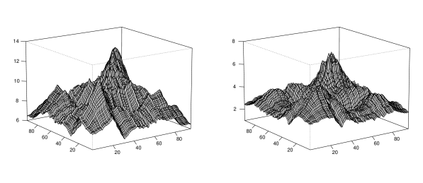
Figure 1: Estimated lag-zero autocovariance kernels of the temperature curves: Summer 2007 (left panel) and summer 2009 (right panel).

To see were the differences between the temperatures in the two summer periods come from and to better interpret the test results, Figure 2 presents a contour plot of the estimated squared differences $|\widehat{c}_{1}(u,v)-\widehat{c}_{2}(u,v)|^{2}$ for different values of $(u,v)$ in the plane $[0,1]^{2}$. Note that the Hilbert-Schmidt distance $\|\widehat{\mathcal{C}}_{1,0}-\widehat{\mathcal{C}}_{2,0}\|_{HS}$ appearing in the test statistic $T_{M}$ can be approximated by the discretized quantity $\sqrt{L^{-2}\sum_{i=1}^{L}\sum_{j=1}^{L}|\widehat{c}_{1}(u_{i},v_{j})-\widehat{c}_{2}(u_{i},v_{j})|^{2}}$, where $L=96$ is the number of equidistant time points in the interval $[0,1]$ used and at which the temperature measurements are recorded. Large values of $|\widehat{c}_{1}(u_{i},v_{j})-\widehat{c}_{2}(u_{i},v_{j})|^{2}$ (i.e., dark gray regions in Figure 2) contribute strongly to the value of the test statistic $T_{M}$ and pinpoint to regions where large differences between the corresponding lag-zero autocovariance operators occur. Taking into account the symmetry of the covariance kernel $c(\cdot,\cdot)$, Figure 2 is very informative. It shows that the main differences between the two covariance operators are concentrated between the time regions 3:00am to 6:00am and 3:00pm to 8:00pm of the daily temperature curves, with the strongest contributions to the test statistic being due to the largest differences recorded around 4:00 to 4:30 in the morning and 6:30 to 7:30 in the evening.

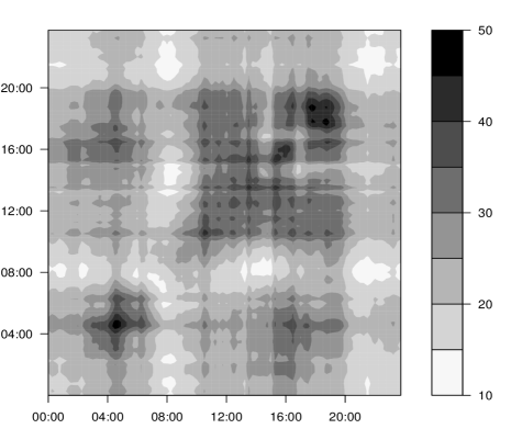
Figure 2: Contour plot of the estimated differences $|\widehat{c}_{1}(u_{i},v_{j})-\widehat{c}_{2}(u_{i},v_{j})|^{2}$ for $(i,j)\in\{1,2,\ldots,96\}$.

5 Appendix : Proofs

In the following we assume, without loss of generality, that $\mu=0$ and we consider the case $h=0$ only. Furthermore, we let $\widehat{\widetilde{\mathcal{C}}}_{0}=n^{-1}\sum_{t=1}^{n}X_{t}\otimes X_{t},$ $Z_{t}=X_{t}\otimes X_{t}-\mathcal{C}_{0},$ $\widehat{Z}_{t}=X_{t}\otimes X_{t}-\widehat{\widetilde{\mathcal{C}}}_{0},$ $\widetilde{Z}_{t}=X_{t}\otimes X_{t},$ $Z_{t,m}=X_{t,m}\otimes X_{t,m}-\mathcal{C}_{0},$ $Z^{*}_{t}=X^{*}_{t}\otimes X^{*}_{t}$ and $\widehat{Z}^{*}_{t}=X^{*}_{t}\otimes X^{*}_{t}-\widehat{\widetilde{\mathcal{C}}}_{0}.$ Also, we denote by $Z_{t}(u,v)$ the kernel of the integral operator $Z_{t},$ i.e., $Z_{t}(u,v)=X_{t}(u)X_{t}(v)-c_{0}(u,v),$ where $c_{0}(u,v)=\mathbb{E}[X_{t}(u)X_{t}(v)],$ and by $Z_{t,m}(u,v)$ the kernel of the integral operator $Z_{t,m},$ i.e., $Z_{t,m}(u,v)=X_{t,m}(u)X_{t,m}(v)-c_{0}(u,v).$

We first fix some notation and present two basic lemmas which will be used in the proofs. Towards this note first that we repeatedly use the fact that, by stationarity, $\mathbb{E}\|X_{t,m}-X_{t}\|^{p}=\mathbb{E}\|X_{0,m}-X_{0}\|^{p}$ and $\mathbb{E}\|X_{t,m}\|^{p}=\mathbb{E}\|X_{t}\|^{p}=\mathbb{E}\|X_{0}\|^{p}$ for $p\in\mathbb{N}$ and for all $t\in\mathbb{Z}.$ Also note that Kokoszka and Reimherr (2013) proved that the $L^{4}$-$m$-approximability of $\mathds{X}$ implies that the tensor product process $\{X_{t}\otimes X_{t},\,t\in\mathbb{Z}\}$ is $L^{2}$-$m$-approximable.

For $X_{t,m}\otimes X_{t,m}$ the $m$-dependent approximation of $X_{t}\otimes X_{t}$, we, therefore, have

$$\sum_{m=1}^{\infty}\bigg{(}\mathbb{E}\|X_{t}\otimes X_{t}-X_{t,m}\otimes X_{t,m}\|_{HS}^{2}\bigg{)}^{1/2}<\infty.$$ (8)

Furthermore, since $\|X_{0}\otimes X_{t}\|_{HS}=\|X_{0}\|\|X_{t}\|$ for all $t\in\mathbb{Z},$ and using Cauchy-Schwarz’s inequality, we get, for all $t\in\mathbb{Z},$

$$\mathbb{E}\|X_{t}\otimes X_{t}-X_{t,m}\otimes X_{t,m}\|_{HS}^{2} \leq 2\mathbb{E}\|X_{t}\otimes(X_{t}-X_{t,m})\|_{HS}^{2}+2\mathbb{E}\|(X_{t}-X_{t,m})\otimes X_{t,m}\|_{HS}^{2}$$

$$\leq 4(\mathbb{E}\|X_{t}\|^{4})^{1/2}(\mathbb{E}\|X_{t}-X_{t,m}\|^{4})^{1/2}.$$

Therefore, by Assumption 1, we get, for all $t\in\mathbb{Z},$

$$\lim_{m\to\infty}m\left(\mathbb{E}\|X_{t}\otimes X_{t}-X_{t,m}\otimes X_{t,m}\|_{HS}^{2}\right)^{1/2}\leq 2(\mathbb{E}\|X_{t}\|^{4})^{1/4}\lim_{m\to\infty}m(\mathbb{E}\|X_{t}-X_{t,m}\|^{4})^{1/4}=0$$ (9)

and by the same arguments,

$$\|\mathbb{E}[X_{0}\otimes X_{t}]\|_{HS}=\|\mathbb{E}[X_{0}\otimes(X_{t}-X_{t,t}]\|_{HS} \leq\left(\mathbb{E}\|X_{0}\|^{2}_{HS}\right)^{1/2}\left(\mathbb{E}\|X_{0}-X_{0,t}\|^{2}_{HS}\right)^{1/2}$$

$$\leq\left(\mathbb{E}\|X_{0}\|^{2}_{HS}\right)^{1/2}\left(\mathbb{E}\|X_{0}-X_{0,t}\|^{4}_{HS}\right)^{1/4}.$$

Therefore, the $L^{4}$-$m$-approximability assumption implies that $\sum_{t\in\mathbb{Z}}\|\mathbb{E}[X_{0}\otimes X_{t}]\|_{HS}<\infty$.

To prove Theorem 2.1, we establish below Lemma 5.1 and Lemma 5.2. Their proofs are given in the supplementary material.

Lemma 5.1.

  Let $g_{b}(\cdot)$ be a non-negative, continuous and bounded function defined on $\mathbb{R}$, satisfying $g_{b}(0)=1$, $g_{b}(u)=g_{b}(-u)$, $g_{b}(u)\leq 1$ for all $u$, $g_{b}(u)=0,$ if $|u|>c,$ for some $c>0.$ Assume that for any fixed $u$, $g_{b}(u)\to 1$ as $n\to\infty.$ Suppose that the process $\mathds{X}$ satisfies Assumption 1 and that $b=b(n)$ is a sequence of integers such that $b^{-1}+bn^{-1/3}=o(1)$ as $n\to\infty.$ Then, as $n\to\infty$,

$$\big{\|}\sum_{s=-b+1}^{b-1}g_{b}(s)\hat{\Gamma}_{s}-\sum_{s=-\infty}^{\infty}\mathbb{E}[Z_{0}\otimes Z_{s}]\big{\|}_{HS}=o_{p}(1),$$

where $\hat{\Gamma}_{s}=\frac{1}{n}\sum_{t=1}^{n-s}\hat{Z}_{t}\otimes\hat{Z}_{t+s}$ for $0\leq s\leq b-1$ and $\hat{\Gamma}_{s}=\frac{1}{n}\sum_{t=1}^{n+s}\hat{Z}_{t-s}\otimes\hat{Z}_{t}$ for $-b+1\leq s<0.$

Lemma 5.2.

Let $g_{b}(\cdot)$ be a non-negative, continuous and bounded function satisfying the conditions of Lemma 5.1. Suppose that $\mathds{X}$ satisfies Assumption 1 and that $b=b(n)$ is a sequence of integers such that $b^{-1}+bn^{-1/2}=o(1)$ as $n\to\infty.$ Then, as $n\to\infty$,

$$\sum_{s=-b+1}^{b-1}g_{b}(s)\dfrac{1}{n}\sum_{t=1}^{n-|s|}\iint Z_{t}(u,v)Z_{t+|s|}(u,v)\mathrm{d}u\mathrm{d}v\overset{P}{\to}\sum_{s=-\infty}^{\infty}\mathbb{E}\iint Z_{0}(u,v)Z_{s}(u,v)\mathrm{d}u\mathrm{d}v.$$

Proof of Theorem 2.1. By the triangle inequality and Theorem $3$ of Kokoszka and Reimherr (2013), the assertion of the theorem is established if we show that, as $n\to\infty,$

$$\sqrt{n}(\hat{\mathcal{C}}_{0}^{*}-\mathbb{E}^{*}(\hat{\mathcal{C}}_{0}^{*}))\Rightarrow\mathcal{Z}_{0},$$ (10)

in probability, where $\mathcal{Z}_{0}$ is a mean zero Gaussian Hilbert Schmidt operator with covariance operator given by

$$\Gamma_{0}=\mathbb{E}[Z_{1}\otimes Z_{1}]+2\sum_{s=2}^{\infty}\mathbb{E}[Z_{1}\otimes Z_{s}].$$

Using Theorem 1 of Horváth et al. (2013), we get

$$\sqrt{n}(\hat{\mathcal{C}}_{0}^{*}- \mathbb{E}^{*}(\hat{\mathcal{C}}_{0}^{*}))$$

$$=\dfrac{1}{\sqrt{n}}\sum_{t=1}^{n}\bigg{[}X_{t}^{*}\otimes X_{t}^{*}-\mathbb{E}^{*}(X_{t}^{*}\otimes X_{t}^{*})-\overline{X}_{n}\otimes(X_{t}^{*}-\mathbb{E}^{*}(X_{t}^{*}))-(X_{t}^{*}-\mathbb{E}^{*}(X_{t}^{*}))\otimes\overline{X}_{n}\bigg{]}$$

$$=\dfrac{1}{\sqrt{n}}\sum_{t=1}^{n}[Z_{t}^{*}-\mathbb{E}^{*}(Z_{t}^{*})]+O_{P}(1/\sqrt{n}).$$

Also note that

$$\dfrac{1}{\sqrt{n}}\sum_{t=1}^{n}[Z_{t}^{*}-\mathbb{E}^{*}(Z_{t}^{*})] =\dfrac{1}{\sqrt{k}}\sum_{t=1}^{k}\left(\dfrac{1}{\sqrt{b}}\sum_{i=1}^{b}\big{(}Z^{*}_{(t-1)b+i}-\mathbb{E}^{*}(Z^{*}_{(t-1)b+i})\big{)}\right)$$

$$=\dfrac{1}{\sqrt{k}}\sum_{t=1}^{k}\widehat{Y}_{t}^{*},$$

with an obvious notation for $\widehat{Y}^{*}_{t},\,t=1,2,\ldots,k$. Recall that due to the block bootstrap resampling scheme, the random variables $\widehat{Y}^{*}_{t},\,t=1,2,\ldots,k,$ are i.i.d. Therefore to prove (10), it suffices by Lemma $5$ of Kokoszka and Reimherr (2013), to prove that,

1. $\left\langle\dfrac{1}{\sqrt{k}}\sum_{t=1}^{k}\widehat{Y}_{t}^{*},y\right\rangle_{HS}\overset{d}{\to}N(0,\sigma^{2}(y))$ for every Hilbert Schmidt operator $y$ acting on $L^{2},$

and that

1. $\lim_{n\to\infty}\mathbb{E}^{*}\left\|\dfrac{1}{\sqrt{k}}\sum_{t=1}^{k}\hat{Y}_{t}^{*}\right\|^{2}_{HS}$ exists and is finite.

To establish assertion (i), we first prove that, as $n\to\infty$,

$$\mathrm{Var}^{*}\left(\left\langle\dfrac{1}{\sqrt{k}}\sum_{t=1}^{k}\widehat{Y}_{t}^{*},y\right\rangle_{HS}\right)\overset{P}{\to}\sigma^{2}(y).$$ (11)

Consider (11) and notice that

$$\mathrm{Var}^{*}\left(\left\langle\dfrac{1}{\sqrt{k}}\sum_{t=1}^{k}\widehat{Y}_{t}^{*},y\right\rangle_{HS}\right)=\mathrm{Var}^{*}\left(\langle\widehat{Y}_{1}^{*},y\rangle_{HS}\right)=\mathbb{E}^{*}\left[\left\langle\dfrac{1}{\sqrt{b}}\sum_{t=1}^{b}(Z^{*}_{t}-\mathbb{E}^{*}(Z^{*}_{t})),y\right\rangle_{HS}\right]^{2}.$$ (12)

Let $N=n-b+1,$ $\widetilde{Y}_{t}=b^{-1/2}(\widetilde{Z}_{t}+\widetilde{Z}_{t+1}+\ldots+\widetilde{Z}_{t+b-1}),$ $t=1,2,\ldots,N$ and $\widetilde{Y}^{*}_{t}=b^{-1/2}\sum_{i=1}^{b}Z^{*}_{(t-1)b+i},$ $t=1,2,\ldots,k.$ Since $n/N\to 1$ as $n\to\infty,$ in the following we will occasionally replace $1/N$ by $1/n.$ Notice that,

$$\mathbb{E}^{*}\left(\left\langle\dfrac{1}{\sqrt{b}}\sum_{t=1}^{b}Z^{*}_{t},y\right\rangle_{HS}\right) =\mathbb{E}^{*}(\widetilde{Y}^{*}_{1})=\dfrac{1}{N}\sum_{t=1}^{N}\langle\widetilde{Y}_{t},y\rangle_{HS}$$

$$=\dfrac{\sqrt{b}}{N}\left[\sum_{t=1}^{n}\langle\tilde{Z}_{t},y\rangle_{HS}-\sum_{i=1}^{b-1}\left(1-\dfrac{i}{b}\right)[\langle\widetilde{Z}_{i},y\rangle_{HS}+\langle\widetilde{Z}_{n-i+1},y\rangle_{HS}]\right]$$

$$=\langle\sqrt{b}\,\hat{\tilde{\mathcal{C}}}_{n},y\rangle-\dfrac{\sqrt{b}}{N}\left[\sum_{i=1}^{b-1}\left(1-\dfrac{i}{b}\right)[\langle\widetilde{Z}_{i},y\rangle_{HS}+\langle\widetilde{Z}_{n-i+1},y\rangle_{HS}]\right].$$ (13)

Therefore,

$$\mathrm{Var}^{*} \left(\left\langle\dfrac{1}{\sqrt{k}}\sum_{t=1}^{k}\widehat{Y}_{t}^{*},y\right\rangle_{HS}\right)$$

$$=\mathbb{E}^{*}\left[\left\langle\dfrac{1}{\sqrt{b}}\sum_{t=1}^{b}\widehat{Z}^{*}_{t},y\right\rangle_{HS}+\dfrac{\sqrt{b}}{N}\left[\sum_{i=1}^{b-1}\left(1-\dfrac{i}{b}\right)[\langle\widetilde{Z}_{i},y\rangle_{HS}+\langle\widetilde{Z}_{n-i+1},y\rangle_{HS}]\right]\right]^{2}$$

$$=\mathbb{E}^{*}\left[\left\langle\dfrac{1}{\sqrt{b}}\sum_{t=1}^{b}\widehat{Z}^{*}_{t},y\right\rangle_{HS}\right]^{2}+\left[\dfrac{\sqrt{b}}{N}\left[\sum_{i=1}^{b-1}\left(1-\dfrac{i}{b}\right)[\langle\widetilde{Z}_{i},y\rangle_{HS}+\langle\widetilde{Z}_{n-i+1},y\rangle_{HS}]\right]\right]^{2}$$

$$\qquad+2\left[\dfrac{\sqrt{b}}{N}\left[\sum_{i=1}^{b-1}\left(1-\dfrac{i}{b}\right)[\langle\widetilde{Z}_{i},y\rangle_{HS}+\langle\widetilde{Z}_{n-i+1},y\rangle_{HS}]\right]\right]\mathbb{E}^{*}\left[\left\langle\dfrac{1}{\sqrt{b}}\sum_{t=1}^{b}\widehat{Z}^{*}_{t},y\right\rangle_{HS}\right]$$

$$=\mathbb{E}^{*}\left[\left\langle\dfrac{1}{\sqrt{b}}\sum_{t=1}^{b}\hat{Z}^{*}_{t},y\right\rangle_{HS}\right]^{2}+O_{P}(b^{3}/n^{2}).$$ (14)

Let $\widehat{Y}_{t}=b^{-1/2}(\widehat{Z}_{t}+\widehat{Z}_{t+1}+\ldots+\widehat{Z}_{t+b-1}),$ $t=1,2,\ldots,N.$ Since,

$$\mathbb{E}^{*} \left[\left\langle\dfrac{1}{\sqrt{b}}\sum_{t=1}^{b}\widehat{Z}^{*}_{t},y\right\rangle_{HS}\right]^{2}=\dfrac{1}{N}\sum_{t=1}^{N}\langle\widehat{Y}_{t},y\rangle_{HS}^{2}$$

$$=\dfrac{1}{N}\sum_{t=1}^{n}\langle\widehat{Z}_{t},y\rangle_{HS}\langle\widehat{Z}_{t},y\rangle_{HS}$$

$$\;+\sum_{i=1}^{b-1}\left(1-\dfrac{i}{b}\right)\dfrac{1}{N}\sum_{t=1}^{n-i}[\langle\widehat{Z}_{t},y\rangle_{HS}\langle\widehat{Z}_{t+i},y\rangle_{HS}+\langle\widehat{Z}_{t+i},y\rangle_{HS}\langle\widehat{Z}_{t},y\rangle_{HS}]$$

$$\;-\dfrac{1}{N}\sum_{i=1}^{b-1}\left(1-\dfrac{i}{b}\right)[\langle\widehat{Z}_{i},y\rangle_{HS}\langle\widehat{Z}_{i},y\rangle_{HS}+\langle\widehat{Z}_{n-i+1},y\rangle_{HS}\langle\widehat{Z}_{n-i+1},y\rangle]_{HS}$$

$$\;-\dfrac{1}{N}\sum_{i=1}^{b-1}\sum_{j=1}^{b-t}\left(1-\dfrac{j+i}{b}\right)[\langle\hat{Z}_{j},y\rangle_{HS}\langle\widehat{Z}_{j+i},y\rangle_{HS}+\langle\widehat{Z}_{n-j+1-i},y\rangle_{HS}\langle\widehat{Z}_{n-j+1},y\rangle_{HS}$$

$$\hskip 105.0pt+\langle\widehat{Z}_{j+i},y\rangle_{HS}\langle\widehat{Z}_{j},y\rangle_{HS}+\langle\widehat{Z}_{n-j+1},y\rangle_{HS}\langle\widehat{Z}_{n-j+1-i},y\rangle_{HS}],$$

we get, using (14),

$$\mathrm{Var}^{*}\left(\left\langle\dfrac{1}{\sqrt{k}}\sum_{t=1}^{k}\widehat{Y}_{t}^{*},y\right\rangle_{HS}\right)$$

$$=\dfrac{1}{N}\sum_{t=1}^{n}\langle\widehat{Z}_{t},y\rangle_{HS}\langle\widehat{Z}_{t},y\rangle_{HS}+\sum_{i=1}^{b-1}\left(1-\dfrac{i}{b}\right)\dfrac{1}{N}\sum_{t=1}^{n-i}[\langle\widehat{Z}_{t},y\rangle_{HS}\langle\widehat{Z}_{t+i},y\rangle_{HS}+\langle\widehat{Z}_{t+i},y\rangle_{HS}\langle\widehat{Z}_{t},y\rangle_{HS}]$$

$$\hskip 280.0pt+O_{P}(b/n)+O_{P}(b^{2}/n)+O_{P}(b^{3}/n^{2}).$$

Therefore,

$$\mathrm{Var}^{*}\left(\left\langle\dfrac{1}{\sqrt{k}}\sum_{t=1}^{k}\widehat{Y}_{t}^{*},y\right\rangle_{HS}\right)$$

$$=\dfrac{1}{N}\sum_{t=1}^{n}\langle\widehat{Z}_{t}\otimes\widehat{Z}_{t},y\otimes y\rangle_{HS}+\sum_{i=1}^{b-1}\left(1-\dfrac{i}{b}\right)\dfrac{1}{N}\sum_{t=1}^{n-i}[\langle\widehat{Z}_{t}\otimes\widehat{Z}_{t+i},y\otimes y\rangle_{HS}+\langle\widehat{Z}_{t+i}\otimes\widehat{Z}_{t},y\otimes y\rangle_{HS}]$$

$$\hskip 340.0pt+O_{P}(b^{2}/n).$$ (15)

Let $g_{b}(i)=\left(1-\frac{|i|}{b}\right)$ in Lemma 5.1, and use the triangular inequality to get

$$\left|\left\langle\dfrac{1}{N}\sum_{t=1}^{n}\widehat{Z}_{t}\otimes\widehat{Z}_{t}+\sum_{i=1}^{b-1}\left(1-\dfrac{i}{b}\right)\dfrac{1}{N}\sum_{t=1}^{n-i}[\widehat{Z}_{t}\otimes\widehat{Z}_{t+i}+\widehat{Z}_{t+i}\otimes\widehat{Z}_{t}]-\sum_{t=-\infty}^{\infty}\mathbb{E}[Z_{0}\otimes Z_{t}],y\otimes y\right\rangle_{HS}\right|$$

$$\hskip 2.0pt\leq\left\|\dfrac{1}{N}\sum_{t=1}^{n}\widehat{Z}_{t}\otimes\widehat{Z}_{t}+\sum_{i=1}^{b-1}\left(1-\dfrac{i}{b}\right)\dfrac{1}{N}\sum_{t=1}^{n-i}[\widehat{Z}_{t}\otimes\widehat{Z}_{t+i}+\widehat{Z}_{t+i}\otimes\widehat{Z}_{t}]-\sum_{t=-\infty}^{\infty}\mathbb{E}[Z_{0}\otimes Z_{t}]\right\|_{HS}\big{\|}y\otimes y\big{\|}_{HS}$$

$$=o_{p}(1).$$

Therefore, and using $\langle Z_{0}\otimes Z_{t},y\otimes y\rangle_{HS}=\langle Z_{0},y\rangle_{HS}\langle Z_{t},y\rangle_{HS}$, we get from (15), as $n\to\infty,$

$$\mathrm{Var}^{*}\left(\left\langle\dfrac{1}{\sqrt{k}}\sum_{t=1}^{k}\widehat{Y}_{t}^{*},y\right\rangle_{HS}\right)\overset{P}{\to}\left\langle\sum_{t=-\infty}^{\infty}\mathbb{E}[Z_{0}\otimes Z_{t}],y\otimes y\right\rangle_{HS}=\langle\Gamma_{0},y\otimes y\rangle_{HS}=\sigma^{2}(y).$$ (16)

We next establish the asymptotic normality stated in (i). Since $\langle\widehat{Y}_{t}^{*},y\rangle_{HS},\,t=1,2,\ldots,k$ are i.i.d. real valued random variables, we show that Lindeberg’s condition is satisfied, i.e., for every $\varepsilon>0,$ as $n\to\infty,$

$$\dfrac{1}{\tau_{k}^{*2}}\sum_{t=1}^{k}\mathbb{E}^{*}\left[\big{(}\langle\widehat{Y}_{t}^{*},y\rangle_{HS}-\mathbb{E}^{*}(\langle\widehat{Y}_{t}^{*},y\rangle_{HS})\big{)}^{2}\mathds{1}\big{(}|\langle\widehat{Y}_{t}^{*},y\rangle_{HS}-E^{*}(\langle\widehat{Y}_{t}^{*},y\rangle_{HS})|>\varepsilon\tau_{k}^{*}\big{)}\right]=o_{p}(1),$$ (17)

where $\mathds{1}_{A}(x)$ denotes the indicator function of the set $A$ and

$$\tau_{k}^{*2}=\sum_{t=1}^{k}\mathrm{Var}^{*}(\langle\widehat{Y}_{t}^{*},y\rangle_{HS})=k\mathrm{Var}^{*}(\langle\widehat{Y}_{1}^{*},y\rangle_{HS}).$$ (18)

To establish (17), and because of (16) and (18), it suffices to show that, for any $\delta>0,$ as $n\to\infty,$

$$P\left(\dfrac{1}{k}\sum_{t=1}^{k}\mathbb{E}^{*}\left[(\langle\widehat{Y}_{t}^{*},y\rangle_{HS}-\mathbb{E}^{*}(\langle\widehat{Y}_{t}^{*},y\rangle_{HS}))^{2}\mathds{1}(|\langle\widehat{Y}_{t}^{*},y\rangle_{HS}-E^{*}(\langle\widehat{Y}_{t}^{*},y\rangle_{HS})|>\varepsilon\tau_{k}^{*})\right]>\delta\right)\to 0.$$ (19)

Towards this, notice first that, for any two random variables $X$ and $Y$ and any $\eta>0,$

$$\mathbb{E}[|X+Y|^{2} \mathds{1}(|X+Y|>\eta)]$$

$$\leq 4\left[\mathbb{E}|X|^{2}\mathds{1}(|X|>\eta/2)+\mathbb{E}|Y|^{2}\mathds{1}(|Y|>\eta/2)\right];$$ (20)

see Lahiri $(2003)$, p. $56$. Since the random variables $\langle\widehat{Y}_{t}^{*},y\rangle_{HS}$ are i.i.d., we get using expression (13) and Markov’s inequality that, as $n\to\infty,$

$$P\left(\dfrac{1}{k}\sum_{t=1}^{k}\mathbb{E}^{*}\left[(\langle\widehat{Y}_{t}^{*},y\rangle_{HS}-\mathbb{E}^{*}(\langle\widehat{Y}_{t}^{*},y\rangle_{HS}))^{2}\mathds{1}(|\langle\widehat{Y}_{t}^{*},y\rangle_{HS}-\mathbb{E}^{*}(\langle\widehat{Y}_{t}^{*},y\rangle_{HS})|>\varepsilon\tau_{k}^{*})\right]>\delta\right)$$

$$\leq\delta^{-1}\mathbb{E}\left\{\mathbb{E}^{*}\left[(\langle\widehat{Y}_{1}^{*},y\rangle_{HS}-\mathbb{E}^{*}(\langle\widehat{Y}_{1}^{*},y\rangle_{HS}))^{2}\mathds{1}(|\langle\widehat{Y}_{1}^{*},y\rangle_{HS}-\mathbb{E}^{*}(\langle\widehat{Y}_{1}^{*},y\rangle_{HS})|>\varepsilon\tau_{k}^{*})\right]\right\}$$

$$=\delta^{-1}\mathbb{E}\Bigg{\{}\mathbb{E}^{*}\Bigg{[}\left(\left\langle\dfrac{1}{\sqrt{b}}\sum_{t=1}^{b}\widehat{Z}^{*}_{t},y\right\rangle_{HS}+\dfrac{\sqrt{b}}{N}\left[\sum_{i=1}^{b-1}\left(1-\dfrac{i}{b}\right)[\langle\widetilde{Z}_{i},y\rangle_{HS}+\langle\widetilde{Z}_{n-i+1},y\rangle_{HS}]\right]\right)^{2}$$

$$\hskip 35.0pt\times\mathds{1}\left(\left|\left\langle\dfrac{1}{\sqrt{b}}\sum_{t=1}^{b}\widehat{Z}^{*}_{t},y\right\rangle_{HS}+\dfrac{\sqrt{b}}{N}\left[\sum_{i=1}^{b-1}\left(1-\dfrac{i}{b}\right)[\langle\widetilde{Z}_{i},y\rangle_{HS}+\langle\widetilde{Z}_{n-i+1},y\rangle_{HS}]\right]\right|>\varepsilon\tau_{k}^{*}\right)\Bigg{]}\Bigg{\}}$$

$$=\delta^{-1}\mathbb{E}\Bigg{[}\dfrac{1}{N}\sum_{t=1}^{N}\left(\langle\widehat{Y}_{t},y\rangle_{HS}+\dfrac{\sqrt{b}}{N}\left[\sum_{i=1}^{b-1}\left(1-\dfrac{i}{b}\right)[\langle\widetilde{Z}_{i},y\rangle_{HS}+\langle\widetilde{Z}_{n-i+1},y\rangle_{HS}]\right]\right)^{2}$$

$$\hskip 35.0pt\times\mathds{1}\left(\left|\langle\widehat{Y}_{t},y\rangle_{HS}+\dfrac{\sqrt{b}}{N}\left[\sum_{i=1}^{b-1}\left(1-\dfrac{i}{b}\right)[\langle\widetilde{Z}_{i},y\rangle_{HS}+\langle\widetilde{Z}_{n-i+1},y\rangle_{HS}]\right]\right|>\varepsilon\tau_{k}^{*}\right)\Bigg{]}$$

$$\leq 4\delta^{-1}\Bigg{[}\mathbb{E}(\langle\widehat{Y}_{1},y\rangle_{HS}^{2})\mathds{1}(|\langle\widehat{Y}_{1},y\rangle_{HS}|>\varepsilon\tau_{k}^{*}/2)+\mathbb{E}\left(\dfrac{\sqrt{b}}{N}\sum_{i=1}^{b-1}\left(1-\dfrac{i}{b}\right)[\langle\widetilde{Z}_{i},y\rangle_{HS}+\langle\widetilde{Z}_{n-i+1},y\rangle_{HS}]\right)^{2}$$

$$\hskip 130.0pt\times\mathds{1}(\left|\left(\dfrac{\sqrt{b}}{N}\sum_{i=1}^{b-1}\left(1-\dfrac{i}{b}\right)[\langle\widetilde{Z}_{i},y\rangle_{HS}+\langle\widetilde{Z}_{n-i+1},y\rangle_{HS}]\right)\right|>\varepsilon\tau_{k}^{*}/2)\Bigg{]}$$

$$\leq 4\delta^{-1}\Bigg{[}\mathbb{E}(\langle\widehat{Y}_{1},y\rangle_{HS}^{2})\mathds{1}(|\langle\widehat{Y}_{1},y\rangle_{HS}|>\varepsilon\tau_{k}^{*}/2)+\mathbb{E}\left(\dfrac{\sqrt{b}}{N}\sum_{i=1}^{b-1}\left(1-\dfrac{i}{b}\right)[\langle\widetilde{Z}_{i},y\rangle_{HS}+\langle\widetilde{Z}_{n-i+1},y\rangle_{HS}]\right)^{2}\Bigg{]}$$

$$\leq 4\delta^{-1}\mathbb{E}(\langle\widehat{Y}_{1},y\rangle_{HS}^{2})\mathds{1}(|\langle\widehat{Y}_{1},y\rangle_{HS}|>\varepsilon\tau_{k}^{*}/2)+O(b^{3}/n^{2}).$$ (21)

By Lemma $4$ of Kokoszka and Reimherr (2013) it follows that $\sum_{s=-\infty}^{\infty}\mathbb{E}\langle Z_{0},y\rangle_{HS}\langle Z_{s},y\rangle_{HS}$ converges absolutely. By Kronecker’s lemma, we then get, as $n\to\infty,$

$$\mathbb{E}(\langle\widehat{Y}_{1},y\rangle_{HS}^{2}) =\dfrac{1}{b}\sum_{i=1}^{b}\sum_{j=1}^{b}\mathbb{E}[\langle\widehat{Z}_{i},y\rangle_{HS}\langle\widehat{Z}_{j},y\rangle_{HS}]$$

$$=\sum_{|s|<b}\left(1-\dfrac{|s|}{b}\right)\mathbb{E}[\langle\widehat{Z}_{0},y\rangle_{HS}\langle\widehat{Z}_{s},y\rangle_{HS}]$$

$$=\sum_{|s|<b}\left(1-\dfrac{|s|}{b}\right)\mathbb{E}[\langle Z_{0},y\rangle_{HS}\langle Z_{s},y\rangle_{HS}]+O(b/n^{1/2})$$

$$\to\sum_{s=-\infty}^{\infty}\mathbb{E}[\langle Z_{0},y\rangle_{HS}\langle Z_{s},y\rangle_{HS}].$$

Therefore, by the dominated convergence theorem,

$$\mathbb{E}[\langle\widehat{Y}_{1},y\rangle_{HS}^{2})\mathds{1}(|\langle\widehat{Y}_{1},y\rangle_{HS}|>\varepsilon\tau_{k}^{*}/2)=o(1)$$ (22)

and, therefore, assertion (i) is proved.

To establish assertion (ii), notice first that

$$\mathbb{E}^{*}\left\|\dfrac{1}{\sqrt{k}}\sum_{t=1}^{k}\widehat{Y}^{*}_{t}\right\|_{HS}^{2}=\mathbb{E}^{*}\|\widehat{Y}^{*}_{1}\|_{HS}^{2}.$$

Furthermore, since

$$\mathbb{E}^{*}\left(\dfrac{1}{\sqrt{b}}\sum_{t=1}^{b}Z_{t}^{*}\right)=\dfrac{1}{N}\sum_{t=1}^{N}\widetilde{Y}_{t} =\dfrac{\sqrt{b}}{N}\left[\sum_{t=1}^{n}\widetilde{Z}_{t}-\sum_{i=1}^{b-1}\left(1-\dfrac{i}{b}\right)[\widetilde{Z}_{i}+\widetilde{Z}_{n-i+1}]\right]$$

$$=\sqrt{b}\widehat{\widetilde{C}}_{n}-\dfrac{\sqrt{b}}{N}\sum_{i=1}^{b-1}\left(1-\dfrac{i}{b}\right)[\widetilde{Z}_{i}+\widetilde{Z}_{n-i+1}],$$

we get

$$\mathbb{E}^{*}\|\widehat{Y}^{*}_{1}\|_{HS}^{2} =\mathbb{E}^{*}\left\|\dfrac{1}{\sqrt{b}}\sum_{t=1}^{b}\widehat{Z}^{*}_{t}+\dfrac{\sqrt{b}}{N}\sum_{i=1}^{b-1}\left(1-\dfrac{i}{b}\right)[\widetilde{Z}_{i}+\widetilde{Z}_{n-i+1}]\right\|_{HS}^{2}$$

$$=\dfrac{1}{N}\sum_{t=1}^{N}\left\|\widehat{Y}_{t}+\dfrac{\sqrt{b}}{N}\sum_{i=1}^{b-1}\left(1-\dfrac{i}{b}\right)[\widetilde{Z}_{i}+\widetilde{Z}_{n-i+1}]\right\|_{HS}^{2}.$$

Since, $\sqrt{b}N^{-1}\sum_{i=1}^{b-1}\left(1-\dfrac{i}{b}\right)[\widetilde{Z}_{i}+\widetilde{Z}_{n-i+1}]=O_{P}(b^{3/2}/n),$ it suffices to prove that the limit

$$\lim_{n\to\infty}\dfrac{1}{N}\sum_{t=1}^{N}\|\widehat{Y}_{t}\|_{HS}^{2}$$ (23)

exists and it is finite. Let $Y_{t}=b^{-1/2}(Z_{t}+\dots+Z_{t+b-1}),\,t=1,2,\ldots N,$ and note that $N^{-1}\sum_{t=1}^{N}\|\widehat{Y}_{t}\|_{HS}^{2}=N^{-1}\sum_{t=1}^{N}\|Y_{t}+\sqrt{b}(\mathcal{C}_{0}-\widehat{\widetilde{\mathcal{C}}}_{0})\|_{HS}^{2}$. By Theorem 3 of Kokoszka and Reimherr (2013), in order to prove (23), it suffices to show that

$$\lim_{n\to\infty}\dfrac{1}{N}\sum_{t=1}^{N}\|Y_{t}\|_{HS}^{2}$$ (24)

exists and it is finite. We have that

$$\dfrac{1}{N}\sum_{t=1}^{N}\|Y_{t}\|_{HS}^{2} =\dfrac{1}{N}\langle Z_{t},Z_{t}\rangle_{HS}+\sum_{i=1}^{b-1}\left(1-\dfrac{i}{b}\right)\dfrac{1}{N}\sum_{t=1}^{n-i}[\langle Z_{t},Z_{t+i}\rangle_{HS}+\langle Z_{t+i},Z_{t}\rangle_{HS}]$$

$$\hskip 20.0pt-\dfrac{1}{N}\sum_{t=1}^{b-1}\left(1-\dfrac{t}{b}\right)[\langle Z_{t},Z_{t}\rangle_{HS}+\langle X_{n-t+1},X_{n-t+1}\rangle]_{HS}$$

$$\hskip 20.0pt-\dfrac{1}{N}\sum_{t=1}^{b-1}\sum_{j=1}^{b-t}\left(1-\dfrac{t+j}{b}\right)[\langle Z_{j},Z_{j+t}\rangle_{HS}+\langle Z_{n-j+1-t},Z_{n-j+1}\rangle_{HS}$$

$$\hskip 145.0pt+\langle Z_{j+t},Z_{j}\rangle_{HS}+\langle Z_{n-j+1},Z_{n-j+1-t}\rangle_{HS}]$$

$$=\dfrac{1}{N}\sum_{t=1}^{n}\langle Z_{t},Z_{t}\rangle_{HS}+\sum_{i=1}^{b-1}\left(1-\dfrac{i}{b}\right)\dfrac{1}{N}\sum_{t=1}^{n-i}[\langle Z_{t},Z_{t+i}\rangle_{HS}+\langle Z_{t+i},Z_{t}\rangle_{HS}]+O_{P}(b^{2}/n)$$

$$=\sum_{i=-b+1}^{b-1}\left(1-\dfrac{i}{b}\right)\dfrac{1}{n}\sum_{t=1}^{n-|i|}\iint Z_{t}(u,v)Z_{t+|i|}(u,v)\mathrm{d}u\mathrm{d}v+O_{P}(b^{2}/n).$$ (25)

Hence, by letting $g_{b}(s)=\left(1-|s|/b\right)$ in Lemma 5.2, we get that the last term above converges to $\sum_{s=-\infty}^{\infty}\mathbb{E}\iint Z_{0}(u,v)Z_{s}(u,v)\mathrm{d}u\mathrm{d}v,$ from which we conclude that, as $n\to\infty$,

$$\mathbb{E}^{*}\|Y^{*}_{1}\|_{HS}^{2}\to\sum_{s=-\infty}^{\infty}\mathbb{E}\iint Z_{0}(u,v)Z_{s}(u,v)\mathrm{d}u\mathrm{d}v,$$

in probability. ∎

Proof of Lemma 3.1. Using Theorem $3$ of Kokoszka and Reimherr (2013) it follows that there exist two independent, mean zero, Gaussian Hilbert Schmidt operators $\mathcal{Z}_{1,0}$ and $\mathcal{Z}_{2,0}$ with covariance operators $\Gamma_{1,0}$ and $\Gamma_{2,0}$ respectively, such that

$$\left(\sqrt{n_{1}}(\widehat{\mathcal{C}}_{1,0}-\mathcal{C}_{1,0}),\sqrt{n_{2}}(\widehat{\mathcal{C}}_{2,0}-\mathcal{C}_{2,0})\right)$$

converges weakly to $(\mathcal{Z}_{1,0},\mathcal{Z}_{2,0}).$ Since

$$\sqrt{\dfrac{n_{1}n_{2}}{M}}(\widehat{\mathcal{C}}_{1,0}-\widehat{\mathcal{C}}_{2,0})=\sqrt{\dfrac{n_{2}}{M}}\sqrt{n_{1}}(\widehat{\mathcal{C}}_{1,0}-\widetilde{\mathcal{C}}_{0})-\sqrt{\dfrac{n_{1}}{M}}\sqrt{n_{2}}(\widehat{\mathcal{C}}_{2,0}-\widetilde{\mathcal{C}}_{0}),$$

where $\widetilde{\mathcal{C}}_{0}$ is the (under $H_{0}$) common lag-zero covariance operator of the two populations, we get that, for $n_{1},n_{2}\to\infty$ and $n_{1}/M\to\theta,$

$$T_{M}\overset{d}{\to}\|\mathcal{Z}_{0}\|^{2}_{HS},$$

where $\mathcal{Z}_{0}=\sqrt{1-\theta}\mathcal{Z}_{1,0}-\sqrt{\theta}\mathcal{Z}_{2,0}.$ ∎

Proof of Theorem 3.1. Using the triangle inequality and the fact that $\sqrt{n}(\widehat{\mathcal{C}}_{i,0}-\mathcal{C}_{i,0})\Rightarrow\mathcal{Z}_{i,0}$, $i=1,2$, it suffices to prove that $T_{M}^{*}$ converges weakly to $\|\mathcal{Z}_{0}\|^{2}_{HS}$, where $\mathcal{Z}_{0}=\sqrt{1-\theta}\mathcal{Z}_{1,0}-\sqrt{\theta}\mathcal{Z}_{2,0}.$ This is proved along the same lines as Lemma 3.1 using of Theorem 2.1 and the independence of the pseudo-random elements $\overline{\mathcal{Y}}_{1,n_{1}}^{*}$ and $\overline{\mathcal{Y}}_{2,n_{2}}^{*}$. ∎

Data Availability Statement

The data that support the findings of this study are available on request from the corresponding author. The data are not publicly available due to privacy or ethical restrictions.

Supplementary Material

The supplementary material contains the proofs of Lemma 5.1 and Lemma 5.2.

References

• [1] Cuevas, A. Febrero, M. and Freiman, R. (2004). An ANOVA test for functional data. Computational Statistics and Data Analysis, Vol. 47, 111–122.
• [2] Fremdt, S., Steinebach, J.G., Horváth, L. and Kokoszka, P. (2013). Testing the equality of covariance operators in functional samples. Scandinavian Journal of Statistics, Vol. 40, 138– 152.
• [3] Hörmann, S. and Kokoszka, P. (2010). Weakly dependent functional data. The Annals of Statistics. Vol. 38, 1845–1884.
• [4] Hörmann, S., Kokoszka, P. and Nisol, G. (2018). Testing for periodicity in functional time series. The Annals of Statistics. Vol. 46, 2960–2984.
• [5] Horváth, L. and Kokoszka, P. (2012). Inference for Functional Data with Applications. New York: Springer-Verlag.
• [6] Horváth, L. and Rice, G. (2015). Testing equality of means when the observations are from functional time series. Journal of Time Series Analysis, Vol. 36, 88–108.
• [7] Horváth, L., Rice, G. and Whipple, S. (2016). Adaptive bandwidth selection in the long run covariance estimator of functional time series. Computational Statistics and Data Analysis, Vol. 100, 676–693.
• [8] Kokoszka, P. and Reimherr, M. (2013). Asymptotic normality of the principal components of functional time series. Stochastic Processes and their Applications, Vol. 123, 1546–1562.
• [9] Künsch, H.R. (1989). The jackknife and the bootstrap for general stationary observations. The Annals of Statistics, Vol. 17, 1217–1261.
• [10] Lahiri, S. (2003). Resampling Methods for Dependent Data. New York: Springer-Verlag.
• [11] Lele, S. and Carlstein, E. (1990). Two-sample bootstrap tests: when to mix? Institute of Statistics Mimeo Series, No. 2031, Department of Statistics, North Carolina State University, USA.
• [12] Liu, R.Y. and Singh, K. (1992). Moving blocks jackknife and bootstrap capture weak dependence. In “Exploring the Limits of the Bootstrap” (R. Lepage and L. Billard, Eds.), pp. 225–248, New York: Wiley.
• [13] Mas, A. (2002). Weak convergence for the covariance operators of a Hilbertian linear process. Stochastic Processes and their Applications, Vol. 99, 117–135.
• [14] Panaretos, V.M., Kraus, D. and Maddocks, J.H. (2010). Second-order comparison of Gaussian random functions and the geometry of DNA minicircles. Journal of the American Statistical Association, Vol. 105, 670–682.
• [15] Paparoditis, E. and Sapatinas, T. (2016). Bootstrap-based testing of equality of mean functions or equality of covariance operators for functional data. Biometrika, Vol. 103, 727–733.
• [16] Pigoli, D., Aston, J.A.D., Dryden, I.L. and Secchi, P. (2014). Distances and inference for covariance operators. Biometrika, Vol. 101, 409–422.
• [17] Politis, D. and Romano, J. (1992). A general resampling scheme for triangular arrays of $\alpha$-mixing random variables with application to the problem of spectral density estimation. The Annals of Statistics, Vol. 20, 1985–2007.
• [18] Rice, G. and Shang, H.L. (2017) A plug-in bandwidth selection procedure for long run covariance estimation with stationary functional time series. Journal of Time Series Analysis, Vol. 38, 591–609.
• [19] Zhang, J.-T. (2013). Analysis of Variance for Functional Data. New York: Chapman & Hall/CRC.
• [20] Zhang, X. and Shao, X. (2015). Two sample inference for the second-order property of temporally dependent functional data. Bernoulli, Vol. 21, 909–929.