MPP-2018-301

DESY 19-002

The Tensor Pomeron and
Low-$x$ Deep Inelastic Scattering

Daniel Britzger ^a,1, Carlo Ewerz ^b,c,d,2, Sasha Glazov ^e,3,
Otto Nachtmann ^b,4, Stefan Schmitt ^e,5

^a Max-Planck-Institut für Physik,
Föhringer Ring 6, D-80805 München, Germany

^b Institut für Theoretische Physik, Universität Heidelberg,
Philosophenweg 16, D-69120 Heidelberg, Germany

^c ExtreMe Matter Institute EMMI, GSI Helmholtzzentrum für Schwerionenforschung,
Planckstraße 1, D-64291 Darmstadt, Germany

^d Frankfurt Institute for Advanced Studies,
Ruth-Moufang-Straße 1, D-60438 Frankfurt, Germany

^e Deutsches Elektronen-Synchrotron DESY,
Notkestraße 85, D-22607 Hamburg, Germany

  ¹ email: britzger@mpp.mpg.de
² email: C.Ewerz@thphys.uni-heidelberg.de
³ email: Alexandre.Glazov@desy.de
⁴ email: O.Nachtmann@thphys.uni-heidelberg.de
⁵ email: Stefan.Schmitt@desy.de

The tensor-pomeron model is applied to low-$x$ deep-inelastic lepton-nucleon scattering and photoproduction. We consider c. m. energies in the range 6 - 318 GeV and $Q^{2}<50\,\mbox{GeV}^{2}$. In addition to the soft tensor pomeron, which has proven quite successful for the description of soft hadronic high-energy reactions, we include a hard tensor pomeron. We also include $f_{2}$-reggeon exchange which turns out to be particularly relevant for real-photon-proton scattering at c. m. energies in the range up to 30 GeV. The combination of these exchanges permits a description of the absorption cross sections of real and virtual photons on the proton in the same framework. In particular, a detailed comparison of this two-tensor-pomeron model with the latest HERA data for $x<0.01$ is made. Our model gives a very good description of the transition from the small-$Q^{2}$ regime where the real or virtual photon behaves hadron-like to the large-$Q^{2}$ regime where hard scattering dominates. Our fit allows us, for instance, a determination of the intercepts of the hard pomeron as $1.3008\,({}^{+73}_{-84})$, of the soft pomeron as $1.0935\,({}^{+76}_{-64})$, and of the $f_{2}$ reggeon. We find that in photoproduction the hard pomeron does not contribute within the errors of the fit. We show that assuming a vector instead of a tensor character for the pomeron leads to the conclusion that it must decouple in real photoproduction.

1 Introduction

In this article we will be concerned with the structure functions of deep-inelastic electron- and positron-proton scattering (DIS). They are given by the absorptive part of the forward virtual Compton amplitude, that is, the amplitude for the elastic scattering of a virtual photon on a proton. The high-energy, or small Bjorken-$x$, behaviour of these structure functions has first been observed experimentally in [1, 2] and has since then been subject of extensive experimental and theoretical research; see for example [3] for a review.

It is not our aim here to address the various theoretical approaches to the small-$x$ structure of the proton. We shall concentrate on a particular aspect of the approach based on Regge theory. In Regge theory, elastic hadron-hadron scattering is dominated, at high energies and small angles, by pomeron exchange. The same applies to total cross sections which, by the optical theorem, are related to the forward scattering amplitudes. For reviews of pomeron physics see [4, 5, 6, 7]. In the application of Regge theory the pomeron has often been assumed to be describable as a vector exchange. For example, the two-pomeron approach to low-$x$ DIS introduced in [8, 9, 10] makes use of two vector pomerons, a hard one and a soft one. However, the assumption of a vector character for the pomeron has problems, as we shall also demonstrate again in the present paper. In [11] it has been argued that in general the pomeron should be a tensor pomeron, that is, an exchange object which can be treated effectively as a rank-2 symmetric tensor. In the present study we use a two-pomeron model with two tensor pomerons, a hard one and a soft one, instead of two vector pomerons. With this model we perform a fit to the available data for photoproduction in the centre-of-mass energy range $6<\sqrt{s}<209\,\mbox{GeV}$ and to the latest HERA data for low-$x$ deep-inelastic lepton-nucleon scattering for centre-of-mass energies in the range 225 - 318 GeV and for $x<0.01$. As we will see, the exchange of a tensor pomeron involves for the virtual photon $\gamma^{*}$-pomeron coupling two functions which are in essence related to the $\gamma^{*}$-proton cross sections $\sigma_{T}$ and $\sigma_{L}$, respectively. It is a special aim of our investigations to fit with our model simultaneously $\sigma_{T}$ and $\sigma_{L}$. Given the large kinematic range and the quality of the experimental data a successful fit using tensor pomerons will therefore be a nontrivial result.

In [11] the tensor pomeron was introduced for soft reactions and many of its properties were derived from comparisons with experiment. Further applications of the tensor-pomeron concept were given for photoproduction of pion pairs in [13] and for a number of exclusive central-production reactions in [14, 15, 16, 17, 18, 19, 20]. In [21] the helicity structure of small-$|t|$ proton-proton elastic scattering was calculated in three models for the pomeron: tensor, vector, and scalar. Comparison with experiment [22] left only the tensor pomeron as a viable option. In the present paper we go beyond the regime of soft scattering, to DIS. In accord with [8] we shall now consider two pomerons, but of the tensor type: a soft one, $\mathbbm{P}_{1}$, which is identical to the tensor pomeron of [11], and a hard one, $\mathbbm{P}_{0}$. From fits to the structure functions of DIS, going down in $Q^{2}$ to photoproduction $(Q^{2}=0)$, we shall be able to extract the properties of $\mathbbm{P}_{0}$ and $\mathbbm{P}_{1}$ and their couplings to virtual photons. Since we shall consider data going down in c. m. energy to around 6 GeV we shall also include $f_{2}$ reggeon ($f_{2R}$) exchange in the theoretical description. Following [11], $f_{2R}$ exchange will also be treated as the effective exchange of a symmetric tensor of rank 2.

A particular aspect relevant to our study concerns real Compton scattering. In this regard we discuss further clear evidence against the hypothesis that the pomeron has vector character. We show that a vector pomeron necessarily decouples in real Compton scattering. A tensor pomeron, in contrast, gives a non-vanishing contribution and can successfully describe the data.

Our paper is organised as follows. In section 2 we review the kinematics of DIS and some general relations for the DIS structure functions. In section 3 our ansatz for the exchange of the tensor pomerons and the $f_{2R}$ reggeon is introduced. The resulting expressions for the real and virtual photon-proton cross sections are derived. The vector pomeron and its decoupling in real Compton scattering are discussed in section 4. Section 5 presents the comparison of our tensor-pomeron model with experimental data. We discuss our findings in Section 6. Section 7 gives our conclusions. Appendix A lists the effective propagators and vertices for the two pomerons and for the $f_{2R}$ reggeon. In appendix B we discuss the formulae for the case of a vector pomeron. In appendix C we present the parametrisations for the coupling functions occurring in our approach. In appendices D, E, and F we give details of our fit procedure and of the fit results.

2 Kinematics and general relations for structure functions in DIS

We want to consider electron- and positron-proton inelastic scattering (fig. 1)

$$e(k)+p(p)\longrightarrow e(k^{\prime})+X(p^{\prime})\,.$$ (2.1)

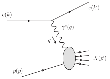
Figure 1: Deep inelastic lepton-proton scattering

The kinematic variables for the reaction (2.1) are standard; see for instance [23]:

$$\begin{split}s&=(p+k)^{2}\,,\\ q&=k-k^{\prime}\,,\\ Q^{2}&=-q^{2}\,,\\ W^{2}&=p^{\prime 2}=(p+q)^{2}\,,\\ \nu&=\frac{p\cdot q}{m_{p}}=\frac{W^{2}+Q^{2}-m_{p}^{2}}{2m_{p}}\,,\\ x&=\frac{Q^{2}}{2m_{p}\nu}=\frac{Q^{2}}{W^{2}+Q^{2}-m_{p}^{2}}\,,\\ y&=\frac{p\cdot q}{p\cdot k}=\frac{W^{2}+Q^{2}-m_{p}^{2}}{s-m_{p}^{2}}\,.\end{split}$$ (2.2)

Furthermore, we define the ratio $\epsilon$ of longitudinal and transverse polarisation strengths of the virtual photon

$$\epsilon=\frac{2(1-y)-y^{2}\delta(W^{2},Q^{2})}{1+(1-y)^{2}+y^{2}\delta(W^{2},Q^{2})}$$ (2.3)

where

$$\delta(W^{2},Q^{2})=\frac{2m_{p}^{2}Q^{2}}{(W^{2}+Q^{2}-m_{p}^{2})^{2}}\,.$$ (2.4)

For given $W^{2}>m^{2}_{p}$ and $Q^{2}\geq 0$ the kinematic limits for $y$ and $\epsilon$ are

$$0\leq y\leq\frac{2}{1+\sqrt{1+2\delta(W^{2},Q^{2})}}$$ (2.5)

corresponding to

$$1\geq\epsilon\geq 0\,.$$ (2.6)

Clearly, for $W^{2}>m^{2}_{p}$ the value $y=0$ ($\epsilon=1$) can only be reached for $s\to\infty$; see (2.2).

The reaction effectively studied in DIS is the absorption of the virtual photon on the proton; see fig. 1.

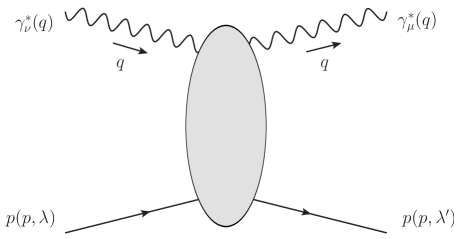
Figure 2: Forward virtual Compton scattering on a proton

The total $\gamma^{*}p$ absorption cross sections are related to the absorptive parts of the virtual forward Compton scattering amplitude. In the following, we shall therefore study the forward virtual Compton scattering on a proton, see fig. 2,

$$\gamma_{\nu}^{*}(q)+p(p,\lambda)\longrightarrow\gamma_{\mu}^{*}(q)+p(p,\lambda^{\prime})\,.$$ (2.7)

The momenta are indicated in brackets and $\lambda,\lambda^{\prime}\in\{1/2,-1/2\}$ are the helicity indices of the protons. We define the amplitude for reaction (2.7) as

$$\mathcal{M}_{\lambda^{\prime}\lambda}^{\mu\nu}(p,q)=\frac{i}{2\pi m_{p}}\int d^{4}x\,e^{-iqx}\langle p(p,\lambda^{\prime})|\mathrm{T}^{*}(J^{\mu}(0)J^{\nu}(x))|p(p,\lambda)\rangle\,.$$ (2.8)

Here $m_{p}$ is the proton mass, $\mathrm{T}^{*}$ denotes the covariantised time-ordered product, and $J^{\mu}(x)$ is the hadronic part of the electromagnetic current. The absorptive part of $\mathcal{M}^{\mu\nu}_{\lambda^{\prime}\lambda}$ (2.8), averaged over the proton helicities, gives the hadronic tensor and the structure functions of DIS,

$$\begin{split}W^{\mu\nu}(p,q)=&\sum_{\lambda^{\prime},\lambda}\frac{1}{2}\,\delta_{\lambda^{\prime}\lambda}\,\frac{1}{2i}\left[\mathcal{M}_{\lambda^{\prime}\lambda}^{\mu\nu}(p,q)-\left(\mathcal{M}_{\lambda\lambda^{\prime}}^{\nu\mu}(p,q)\right)^{*}\right]\\ =&{}\>W_{1}(\nu,Q^{2})\left(-g^{\mu\nu}+\frac{q^{\mu}q^{\nu}}{q^{2}}\right)\\ &+\frac{1}{m_{p}^{2}}\,W_{2}(\nu,Q^{2})\left(p^{\mu}-\frac{p\cdot q}{q^{2}}\,q^{\mu}\right)\left(p^{\nu}-\frac{p\cdot q}{q^{2}}\,q^{\nu}\right).\end{split}$$ (2.9)

We shall also use the total $\gamma^{*}p$ absorption cross sections $\sigma_{T}$ and $\sigma_{L}$ for transversely and longitudinally polarised virtual photons. With $e>0$ the proton charge and Hand’s convention for the flux factor [24] these read

$$\begin{split}\sigma_{T}(W^{2},Q^{2})&=\frac{2\pi m_{p}}{W^{2}-m_{p}^{2}}\,e^{2}W_{1}(\nu,Q^{2})\,,\\ \sigma_{L}(W^{2},Q^{2})&=\frac{2\pi m_{p}}{W^{2}-m_{p}^{2}}\,e^{2}\left[W_{2}(\nu,Q^{2})\frac{\nu^{2}+Q^{2}}{Q^{2}}-W_{1}(\nu,Q^{2})\right]\,.\end{split}$$ (2.10)

3 Structure functions in the tensor-pomeron approach

We shall now assume that for large $W^{2}$, respectively small $x$, the virtual Compton amplitude (2.8) is dominated by the exchange of the two pomerons, $\mathbbm{P}_{0}$ and $\mathbbm{P}_{1}$, plus the $f_{2R}$ reggeon; see fig. 3.

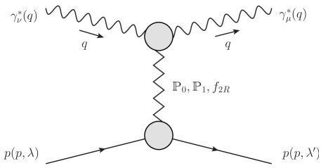
Figure 3: Low-$x$ forward virtual Compton scattering with exchange of the soft ($\mathbbm{P}_{1}$) and hard ($\mathbbm{P}_{0}$) pomeron plus the $f_{2R}$ reggeon.

In order to calculate the diagram shown there we need the effective propagators for $\mathbbm{P}_{0}$ and $\mathbbm{P}_{1}$ as well as the vertex functions $\mathbbm{P}_{j}pp$ and ${\mathbbm{P}}_{j}\gamma^{*}\gamma^{*}$ ($j=0,1$), and the analogous quantities for $f_{2R}$. Our ansätze for these quantities are listed in appendix A. It is now straightforward to calculate the analytic expression corresponding to the diagram of fig. 3. Since all three exchanges are tensor exchanges, the resulting expressions have a similar structure. We find

$$\begin{split}i\,2\pi\,m_{p}e^{2}\mathcal{M}_{\lambda^{\prime}\lambda}^{\mu\nu}(p,q)=&\sum_{j=0,1}g^{\mu\mu^{\prime}}g^{\nu\nu^{\prime}}i\Gamma_{\mu^{\prime}\nu^{\prime}\kappa\rho}^{(\mathbbm{P}_{j}\gamma^{*}\gamma^{*})}(q,q)\,i\Delta^{(P_{j})\,\kappa\rho,\kappa^{\prime}\rho^{\prime}}(W^{2},0)\,\\ &\qquad\times\bar{u}(p,\lambda^{\prime})\,i\Gamma_{\kappa^{\prime}\rho^{\prime}}^{(\mathbbm{P}_{j}pp)}(p,p)\,u(p,\lambda)\\ &+g^{\mu\mu^{\prime}}g^{\nu\nu^{\prime}}i\Gamma_{\mu^{\prime}\nu^{\prime}\kappa\rho}^{(f_{2R}\gamma^{*}\gamma^{*})}(q,q)\,i\Delta^{(f_{2R})\,\kappa\rho,\kappa^{\prime}\rho^{\prime}}(W^{2},0)\,\\ &\qquad\times\bar{u}(p,\lambda^{\prime})\,i\Gamma_{\kappa^{\prime}\rho^{\prime}}^{(f_{2R}pp)}(p,p)\,u(p,\lambda)\,.\end{split}$$ (3.1)

With the expressions from appendix A we obtain

$$\begin{split}\mathcal{M}_{\lambda^{\prime}\lambda}^{\mu\nu}(p,q)&=\frac{1}{2\pi m_{p}}\,\delta_{\lambda^{\prime}\lambda}\sum_{j=0,1,2}\left[2\hat{a}_{j}(Q^{2})\,\Gamma^{(0)\mu\nu\kappa\rho}(q,-q)-\hat{b}_{j}(Q^{2})\,\Gamma^{(2)\mu\nu\kappa\rho}(q,-q)\right]\\ &\quad\times(-i\,3\beta_{jpp})(-iW^{2}\tilde{\alpha}^{\prime}_{j})^{\epsilon_{j}}\frac{1}{2W^{2}}\,(4p_{\kappa}p_{\rho}-g_{\kappa\rho}m_{p}^{2})\,.\end{split}$$ (3.2)

The meaning of the quantities occurring here and in the following is summarised in table 1. The detailed behaviour of the $\gamma^{*}\gamma^{*}$ coupling functions is not predicted by the model. They are assumed to be smooth functions of $Q^{2}$ and will be parametrised with the help of spline functions. Note that quantities with indices $j=0,1,$ and $2$ always refer to the hard pomeron, the soft pomeron, and the $f_{2R}$ reggeon, respectively. The tensor functions $\Gamma^{(l)\mu\nu\kappa\rho}$ ($l=0,2$) are defined in (A.13), (A).

	hard pomeron $\mathbbm{P}_{0}$	soft pomeron $\mathbbm{P}_{1}$	reggeon $f_{2R}$
intercept	$\alpha_{0}(0)=1+\epsilon_{0}$	$\alpha_{1}(0)=1+\epsilon_{1}$	$\alpha_{2}(0)=1+\epsilon_{2}$
slope parameter	$\alpha^{\prime}_{0}$	$\alpha^{\prime}_{1}$	$\alpha^{\prime}_{2}$
$W^{2}$ parameter	$\tilde{\alpha}^{\prime}_{0}$	$\tilde{\alpha}^{\prime}_{1}$	$\tilde{\alpha}^{\prime}_{2}$
$pp$ coupling parameter	$\beta_{0pp}$	$\beta_{1pp}$	$\beta_{2pp}$
$\gamma^{*}\gamma^{*}$ coupling functions	$\hat{a}_{0}(Q^{2})$, $\hat{b}_{0}(Q^{2})$	$\hat{a}_{1}(Q^{2})$, $\hat{b}_{1}(Q^{2})$	$\hat{a}_{2}(Q^{2})$, $\hat{b}_{2}(Q^{2})$

Table 1: Notation for the parameters of our ansatz with hard and soft pomeron and $f_{2R}$ reggeon exchange. The propagators and vertices containing these parameters are given in detail in appendix A.

Using (2.9) we get from (3.2)

$$\begin{split}W_{\mu\nu}(p,q)=&\,\frac{1}{2\pi m_{p}W^{2}}\sum_{j=0,1,2}3\beta_{jpp}(W^{2}\tilde{\alpha}^{\prime}_{j})^{\epsilon_{j}}\cos\left(\frac{\pi}{2}\,\epsilon_{j}\right)\\ &{}\times\left\{\left(-g_{\mu\nu}+\frac{q_{\mu}q_{\nu}}{q^{2}}\right)\Big{[}\hat{b}_{j}(Q^{2})\left(4(p\cdot q)^{2}-2q^{2}m_{p}^{2}\right)\right.\\ &\qquad\qquad\qquad\qquad\quad-2\hat{a}_{j}(Q^{2})(-q^{2})\left(4(p\cdot q)^{2}-q^{2}m_{p}^{2}\right)\Big{]}\\ &{}\qquad\left.+\left(p^{\mu}-\frac{p\cdot q}{q^{2}}\,q^{\mu}\right)\left(p^{\nu}-\frac{p\cdot q}{q^{2}}\,q^{\nu}\right)(-4q^{2})\hat{b}_{j}(Q^{2})\right\},\end{split}$$ (3.3)

such that

$$\begin{split}W_{1}(\nu,Q^{2})=&\,\frac{1}{2\pi m_{p}W^{2}}\sum_{j=0,1,2}3\beta_{jpp}(W^{2}\tilde{\alpha}^{\prime}_{j})^{\epsilon_{j}}\cos\left(\frac{\pi}{2}\,\epsilon_{j}\right)\\ &\times\left[\hat{b}_{j}(Q^{2})\left(4(p\cdot q)^{2}+2Q^{2}m_{p}^{2}\right)-2Q^{2}\hat{a}_{j}(Q^{2})\left(4(p\cdot q)^{2}+Q^{2}m_{p}^{2}\right)\right]\end{split}$$ (3.4)

and

$$W_{2}(\nu,Q^{2})=\,\frac{m_{p}}{2\pi W^{2}}\sum_{j=0,1,2}3\beta_{jpp}(W^{2}\tilde{\alpha}^{\prime}_{j})^{\epsilon_{j}}\cos\left(\frac{\pi}{2}\,\epsilon_{j}\right)4Q^{2}\hat{b}_{j}(Q^{2})\,.$$ (3.5)

Writing $W_{1}$ (3.4) in terms of the variables $Q^{2}$ and $W^{2}$ we get

$$\begin{split}W_{1}(\nu,Q^{2})=&\,\frac{(W^{2}-m_{p}^{2})^{2}}{2\pi m_{p}W^{2}}\sum_{j=0,1,2}3\beta_{jpp}(W^{2}\tilde{\alpha}^{\prime}_{j})^{\epsilon_{j}}\cos\left(\frac{\pi}{2}\,\epsilon_{j}\right)\\ &\times\left\{\hat{b}_{j}(Q^{2})\left[1+\frac{2Q^{2}}{W^{2}-m_{p}^{2}}+\frac{Q^{2}(Q^{2}+2m_{p}^{2})}{(W^{2}-m_{p}^{2})^{2}}\right]\right.\\ &\qquad\left.-2Q^{2}\hat{a}_{j}(Q^{2})\left[1+\frac{2Q^{2}}{W^{2}-m_{p}^{2}}+\frac{Q^{2}(Q^{2}+m_{p}^{2})}{(W^{2}-m_{p}^{2})^{2}}\right]\right\}.\end{split}$$ (3.6)

From (3.5) and (3.6) we get for $\sigma_{T}$ and $\sigma_{L}$ (2.10) with $\alpha_{\rm em}=e^{2}/(4\pi)$, the fine structure constant,

$$\sigma_{T}(W^{2},Q^{2})= \,4\pi\alpha_{\rm em}\,\frac{W^{2}-m_{p}^{2}}{W^{2}}\sum_{j=0,1,2}3\beta_{jpp}(W^{2}\tilde{\alpha}^{\prime}_{j})^{\epsilon_{j}}\cos\left(\frac{\pi}{2}\,\epsilon_{j}\right)$$

$$\times\left\{\hat{b}_{j}(Q^{2})\left[1+\frac{2Q^{2}}{W^{2}-m_{p}^{2}}+\frac{Q^{2}(Q^{2}+2m_{p}^{2})}{(W^{2}-m_{p}^{2})^{2}}\right]\right.$$ (3.7)

$$\qquad\left.-2Q^{2}\hat{a}_{j}(Q^{2})\left[1+\frac{2Q^{2}}{W^{2}-m_{p}^{2}}+\frac{Q^{2}(Q^{2}+m_{p}^{2})}{(W^{2}-m_{p}^{2})^{2}}\right]\right\},$$

$$\sigma_{L}(W^{2},Q^{2})= \,4\pi\alpha_{\rm em}\,\frac{W^{2}-m_{p}^{2}}{W^{2}}\,Q^{2}\sum_{j=0,1,2}3\beta_{jpp}(W^{2}\tilde{\alpha}^{\prime}_{j})^{\epsilon_{j}}\cos\left(\frac{\pi}{2}\,\epsilon_{j}\right)$$ (3.8)

$$\times\left\{2\hat{a}_{j}(Q^{2})\left[1+\frac{2Q^{2}}{W^{2}-m_{p}^{2}}+\frac{Q^{2}(Q^{2}+m_{p}^{2})}{(W^{2}-m_{p}^{2})^{2}}\right]+\hat{b}_{j}(Q^{2})\frac{2m_{p}^{2}}{(W^{2}-m_{p}^{2})^{2}}\right\}.$$

From (3) and (3.8) we finally get for the structure functions $F_{2}=\nu W_{2}$ and $F_{L}$

$$F_{2}(W^{2},Q^{2})= \,\frac{Q^{2}}{4\pi^{2}\alpha_{\rm em}}(1-x)\left[1+2\delta(W^{2},Q^{2})\right]^{-1}\left[\sigma_{T}(W^{2},Q^{2})+\sigma_{L}(W^{2},Q^{2})\right]$$

$$= \,\frac{Q^{2}}{\pi}\,(1-x)\left[1+2\delta(W^{2},Q^{2})\right]^{-1}$$

$$\,\times\frac{W^{2}-m_{p}^{2}}{W^{2}}\sum_{j=0,1,2}3\beta_{jpp}(W^{2}\tilde{\alpha}^{\prime}_{j})^{\epsilon_{j}}\cos\left(\frac{\pi}{2}\,\epsilon_{j}\right)$$ (3.9)

$$\,\times\hat{b}_{j}(Q^{2})\left[1+\frac{2Q^{2}}{W^{2}-m_{p}^{2}}+\frac{Q^{2}(Q^{2}+4m_{p}^{2})}{(W^{2}-m_{p}^{2})^{2}}\right],$$

$$F_{L}(W^{2},Q^{2})= \,\frac{Q^{2}}{4\pi^{2}\alpha_{\rm em}}(1-x)\sigma_{L}(W^{2},Q^{2})$$

$$= \,\frac{Q^{4}}{\pi}\,(1-x)\,\frac{W^{2}-m_{p}^{2}}{W^{2}}\sum_{j=0,1,2}3\beta_{jpp}(W^{2}\tilde{\alpha}^{\prime}_{j})^{\epsilon_{j}}\cos\left(\frac{\pi}{2}\,\epsilon_{j}\right)$$ (3.10)

$$\,\times\left\{2\hat{a}_{j}(Q^{2})\left[1+\frac{2Q^{2}}{W^{2}-m_{p}^{2}}+\frac{Q^{2}(Q^{2}+m_{p}^{2})}{(W^{2}-m_{p}^{2})^{2}}\right]+\hat{b}_{j}(Q^{2})\frac{2m_{p}^{2}}{(W^{2}-m_{p}^{2})^{2}}\right\}.$$

Let us now discuss our results (3.2)-(3). We first note that with our ansatz for the soft and hard pomeron plus $f_{2R}$ reggeon all gauge-invariance relations for the virtual Compton amplitude are satisfied. Indeed, we find from (3.2) and (A.16)

$$\begin{split}q_{\mu}\mathcal{M}_{\lambda^{\prime}\lambda}^{\mu\nu}(p,q)&=0\,,\\ q_{\nu}\mathcal{M}_{\lambda^{\prime}\lambda}^{\mu\nu}(p,q)&=0\,.\end{split}$$ (3.11)

Also, $\sigma_{L}(W^{2},Q^{2})$ vanishes proportional to $Q^{2}$ for $Q^{2}\to 0$, whereas $\sigma_{T}(W^{2},0)$ gives the pomeron plus $f_{2R}$ reggeon part of the total $\gamma p$ cross section for real photons,

$$\begin{split}\sigma_{T}(W^{2},0)&=\sigma_{\gamma p}(W^{2})\\ &=4\pi\alpha_{\rm em}\,\frac{W^{2}-m_{p}^{2}}{W^{2}}\sum_{j=0,1,2}3\beta_{jpp}(W^{2}\tilde{\alpha}^{\prime}_{j})^{\epsilon_{j}}\cos\left(\frac{\pi}{2}\,\epsilon_{j}\right)\hat{b}_{j}(0)\,.\end{split}$$ (3.12)

For this soft process the contributions from the soft pomeron $\mathbbm{P}_{1}$ ($j=1$) plus $f_{2R}$ reggeon ($j=2$) are expected to dominate.

For large $Q^{2}$, on the other hand, we expect the hard pomeron $\mathbbm{P}_{0}$ to give the main contribution to $\sigma_{T}$ and $\sigma_{L}$. For

$$W^{2}\gg Q^{2}\gg m_{p}^{2}$$ (3.13)

we get, therefore, from (3) and (3.8) the following approximate relations:

$$\sigma_{T}(W^{2},Q^{2}) \cong\,4\pi\alpha_{\rm em}\,3\beta_{0pp}(W^{2}\tilde{\alpha}^{\prime}_{0})^{\epsilon_{0}}\cos\left(\frac{\pi}{2}\,\epsilon_{0}\right)\left[\hat{b}_{0}(Q^{2})-2Q^{2}\hat{a}_{0}(Q^{2})\right],$$ (3.14)

$$\sigma_{L}(W^{2},Q^{2}) \cong\,4\pi\alpha_{\rm em}\,Q^{2}\,3\beta_{0pp}(W^{2}\tilde{\alpha}^{\prime}_{0})^{\epsilon_{0}}\cos\left(\frac{\pi}{2}\,\epsilon_{0}\right)2\hat{a}_{0}(Q^{2})\,,$$ (3.15)

and

$$\frac{\sigma_{L}(W^{2},Q^{2})}{\sigma_{T}(W^{2},Q^{2})}\cong\frac{2Q^{2}\hat{a}_{0}(Q^{2})}{\hat{b}_{0}(Q^{2})-2Q^{2}\hat{a}_{0}(Q^{2})}\,.$$ (3.16)

This shows that in the limit (3.13) $\sigma_{L}(W^{2},Q^{2})$ determines the function $\hat{a}_{0}(Q^{2})$ while $\sigma_{T}(W^{2},Q^{2})+\sigma_{L}(W^{2},Q^{2})$ determines the function $\hat{b}_{0}(Q^{2})$.

4 Compton amplitude and vector pomeron

In this section we shall show that for real Compton scattering on a proton the exchange of a vector-type pomeron $\mathbbm{P}_{V}$ gives an amplitude that vanishes identically. We investigate the reaction

$$\gamma(q,\varepsilon)+p(p,\lambda)\longrightarrow\gamma(q^{\prime},\varepsilon^{\prime})+p(p^{\prime},\lambda^{\prime})$$ (4.1)

for real photons, $q^{2}=q^{\prime 2}=0$, and consider the diagram of fig. 4 with vector pomeron exchange.

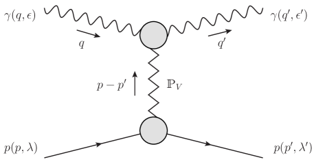
Figure 4: Real Compton scattering on a proton with exchange of a vector pomeron $\mathbbm{P}_{V}$.

The kinematic variables are the c. m. energy $W$ and the momentum transfer squared,

$$\begin{split}W^{2}&=(p+q)^{2}=(p^{\prime}+q^{\prime})^{2}\,,\\ t&=(p-p^{\prime})^{2}=(q^{\prime}-q)^{2}\,.\end{split}$$ (4.2)

The $\mathbbm{P}_{V}pp$ vertex and the $\mathbbm{P}_{V}$ propagator are standard; see e. g. appendix B of [14] and (B.1), (B.2) of the present paper. The important task is to find the structure of the $\mathbbm{P}_{V}\gamma\gamma$ vertex. Using the constraints of Bose symmetry for the photons, of gauge invariance, and of parity conservation in the strong and electromagnetic interactions we derive in appendix B for the $\mathbbm{P}_{V}\gamma\gamma$ vertex function the expression

$$\begin{split}\Gamma_{\mu\nu\rho}^{(\mathbbm{P}_{V}\gamma\gamma)}(q^{\prime},-q)=&{}\,\hat{A}_{2}(t)\left[q^{\prime}_{\mu}(-q^{\prime}_{\nu}q_{\rho}+(q^{\prime}\cdot q)g_{\nu\rho})-(-q_{\mu}q^{\prime}_{\rho}+(q^{\prime}\cdot q)g_{\mu\rho})q_{\nu}\right]\\ &-\hat{A}_{3}(t)\,q^{\prime}_{\mu}q_{\nu}(q^{\prime}_{\rho}-q_{\rho})\\ &+\hat{A}_{4}(t)\,(-q_{\mu}q^{\prime}_{\nu}+(q^{\prime}\cdot q)g_{\mu\nu})(q^{\prime}_{\rho}-q_{\rho})\,.\end{split}$$ (4.3)

Here $\mu$, $\nu$, and $\rho$ are the Lorentz indices for the outgoing photon, the incoming photon, and the vector pomeron $\mathbbm{P}_{V}$, respectively. The $\hat{A}_{j}(t)$ ($j=2,3,4$) are invariant functions.

Applying now (B.1), (B.2), and (4.3) to the amplitude for reaction (4.1) we find from the diagram of fig. 4

$$\begin{split}\langle\gamma(q^{\prime},\varepsilon^{\prime}),p(p^{\prime},\lambda^{\prime})|\mathcal{T}|\gamma(q,\varepsilon),p(p,\lambda)\rangle^{\mathbbm{P}_{V}}=&-\varepsilon^{\prime*\mu}\,\Gamma_{\mu\nu\rho}^{(\mathbbm{P}_{V}\gamma\gamma)}(q^{\prime},-q)\,\varepsilon^{\nu}\Delta^{(\mathbbm{P}_{V})\rho\sigma}(W^{2},t)\\ &\times\bar{u}_{\lambda^{\prime}}(p^{\prime})\Gamma_{\sigma}^{(\mathbbm{P}_{V}pp)}(p^{\prime},p)u_{\lambda}(p)\\ =&\,0\,.\end{split}$$ (4.4)

Here we have used

$$q^{\prime}\cdot\varepsilon^{\prime}=0\,,\qquad q\cdot\varepsilon=0$$ (4.5)

and

$$(q^{\prime}-q)^{\rho}\,\bar{u}_{\lambda^{\prime}}(p^{\prime})\gamma_{\rho}u_{\lambda}(p)=(p-p^{\prime})^{\rho}\,\bar{u}_{\lambda^{\prime}}(p^{\prime})\gamma_{\rho}u_{\lambda}(p)=0\,.$$ (4.6)

The vector pomeron exchange hence gives zero contribution for real Compton scattering. In particular, this implies that a vector pomeron exchange cannot contribute to the total photoabsorption cross section $\sigma_{\gamma p}(W^{2})$ which is proportional to the absorptive part of the forward Compton amplitude. On the other hand, we see from (3.12) that our tensor exchanges give non-zero contributions to $\sigma_{\gamma p}$ for $\hat{b}_{j}(0)\neq 0$. And this will indeed be the case in our fits shown in section 5 below. We think that the decoupling of a vector pomeron in real Compton scattering is another strong argument against treating the pomeron as an effective vector exchange. We note that this vector pomeron decoupling is closely related to the famous Landau-Yang theorem [25, 26] which says that a massive vector particle cannot decay to two real photons; see appendix B.

5 Comparison with experiment

In this section we compare our theoretical ansatz for the tensor-pomeron and $f_{2R}$-reggeon exchanges, as explained in section 3, to experiment by making a global fit. For this fit we use the HERA inclusive DIS data [27] from four different centre-of-mass energies, $\sqrt{s}=225,251,300$, and $318\,\mathrm{GeV}$. We require

$$Q^{2}<50\,\mathrm{GeV}^{2}\qquad\mathrm{and}\qquad x<0.01\,.$$ (5.1)

For the photoproduction cross section we use the measurements from H1 [28] at $W=200\,\mathrm{GeV}$ and ZEUS [29] at $W=209\,\mathrm{GeV}$. In addition, we include in the analysis data at intermediate $W$ ($40\,\mbox{GeV}<W<150\,\mbox{GeV}$) from astroparticle observations [30] and at low $W$ ($6\,\mbox{GeV}<W<19\,\mbox{GeV}$) from a tagged-photon experiment at Fermilab [31].

The directly measured quantity at HERA is the reduced cross section defined as

$$\sigma_{\rm red}(W^{2},Q^{2},y)=\frac{Q^{4}x}{2\pi\alpha_{\rm em}^{2}[1+(1-y)^{2}]}\,\frac{d^{2}\sigma}{dx\,dQ^{2}}(ep\to eX)\,.$$ (5.2)

Expressing this in terms of $\sigma_{T}$ and $\sigma_{L}$ (2.10) we get

$$\begin{split}\sigma_{\rm red}(W^{2},Q^{2},y)=&{}\,\frac{1+(1-y)^{2}+y^{2}\delta(W^{2},Q^{2})}{1+(1-y)^{2}}\,[1+2\delta(W^{2},Q^{2})]^{-1}\frac{Q^{2}}{4\pi^{2}\alpha_{\rm em}}\,(1-x)\\ &\times\left[\sigma_{T}(W^{2},Q^{2})+\sigma_{L}(W^{2},Q^{2})-\tilde{f}(W^{2},Q^{2},y)\,\sigma_{L}(W^{2},Q^{2})\right],\end{split}$$ (5.3)

where

$$\tilde{f}(W^{2},Q^{2},y)=1-\epsilon=\frac{y^{2}[1+2\delta(W^{2},Q^{2})]}{1+(1-y)^{2}+y^{2}\delta(W^{2},Q^{2})}\,.$$ (5.4)

Alternatively, we can express $\sigma_{\rm red}$ through the structure functions (3), (3),

$$\begin{split}\sigma_{\rm red}(W^{2},Q^{2},y)=&\,\frac{1+(1-y)^{2}+y^{2}\delta(W^{2},Q^{2})}{1+(1-y)^{2}}\\ &\times\left\{F_{2}(W^{2},Q^{2})-\tilde{f}(W^{2},Q^{2},y)[1+2\delta(W^{2},Q^{2})]^{-1}F_{L}(W^{2},Q^{2})\right\}.\end{split}$$ (5.5)

Now we discuss the parameters of our model, cf. table 1. For the soft pomeron $\mathbbm{P}_{1}$ we take the default values from (A.3) for

$$\alpha^{\prime}_{1}=\tilde{\alpha}^{\prime}_{1}=0.25\,\mathrm{GeV}^{-2}$$ (5.6)

and leave

$$\epsilon_{1}=\alpha_{1}(0)-1$$ (5.7)

as a fit parameter. The $\mathbbm{P}_{1}pp$ coupling parameter $\beta_{1pp}$ is fixed to (A.11). For our hard pomeron $\mathbbm{P}_{0}$ we also use, for lack of better information,

$$\begin{gathered}\alpha^{\prime}_{0}=\tilde{\alpha}^{\prime}_{0}=0.25\,\mathrm{GeV}^{-2}\,,\\ \beta_{0pp}=\beta_{1pp}=1.87\,\mathrm{GeV}^{-1}\end{gathered}$$ (5.8)

and leave

$$\epsilon_{0}=\alpha_{0}(0)-1$$ (5.9)

as a fit parameter. The pomeron-$\gamma^{*}\gamma^{*}$ coupling functions

$$\hat{a}_{j}(Q^{2})\quad\mbox{and}\quad\hat{b}_{j}(Q^{2})\qquad(j=0,1)$$ (5.10)

are determined from the fit. These functions are parametrised with the help of cubic splines as explained in appendix C. Note that only the products

$$\beta_{jpp}\,\hat{a}_{j}(Q^{2})\quad\mbox{and}\quad\beta_{jpp}\,\hat{b}_{j}(Q^{2})$$ (5.11)

can be determined from our reaction. For $f_{2R}$ exchange we leave $\alpha_{2}(0)=1+\epsilon_{2}$ as fit parameter and use for $\alpha^{\prime}_{2}$, $\tilde{\alpha}^{\prime}_{2}$, $\beta_{2pp}$ the default values from (A.22), (A.25), (A.26). The function $\hat{b}_{2}(Q^{2})$, parametrised according to (C.2), is determined from the fit. The function $\hat{a}_{2}(Q^{2})$ is set to zero, which is justified in our case since for the photoproduction cross section $\hat{a}_{2}(0)$ does not contribute; see (3.12). For $Q^{2}>0$, on the other hand, the data to which we fit are at sufficiently high $W$ such that the whole contribution of the $f_{2R}$ exchange is very small there. With $\hat{a}_{2}(Q^{2})=0$ we neglect in essence the possible $f_{2R}$-exchange contribution to $\sigma_{L}$; see (3.8). The fit parameters for the pomeron and $f_{2R}$ reggeon properties are summarised in table 2.

	parameter	default value used	fit result
$\mathbbm{P}_{0}$	intercept		$\alpha_{0}(0)=1+\epsilon_{0}$
			$\epsilon_{0}=0.3008\,({}^{+73}_{-84})$
	slope parameter	$\alpha^{\prime}_{0}=0.25\,\mbox{GeV}^{-2}$
	$W^{2}$ parameter	$\tilde{\alpha}^{\prime}_{0}=0.25\,\mbox{GeV}^{-2}$
	$pp$ coupling parameter	$\beta_{0pp}=1.87\,\mbox{GeV}^{-1}$
$\mathbbm{P}_{1}$	intercept		$\alpha_{1}(0)=1+\epsilon_{1}$
			$\epsilon_{1}=0.0935\,({}^{+76}_{-64})$
	slope parameter	$\alpha^{\prime}_{1}=0.25\,\mbox{GeV}^{-2}$
	$W^{2}$ parameter	$\tilde{\alpha}^{\prime}_{1}=0.25\,\mbox{GeV}^{-2}$
	$pp$ coupling parameter	$\beta_{1pp}=1.87\,\mbox{GeV}^{-1}$
$f_{2R}$	intercept		$\alpha_{2}(0)=0.485\,({}^{+88}_{-90})$
	slope parameter	$\alpha^{\prime}_{2}=0.9\,\mbox{GeV}^{-2}$
	$W^{2}$ parameter	$\tilde{\alpha}^{\prime}_{2}=0.9\,\mbox{GeV}^{-2}$
	$pp$ coupling parameter	$\beta_{2pp}=3.68\,\mbox{GeV}^{-1}$

Table 2: Fit values obtained for the pomeron and $f_{2R}$ reggeon intercepts and default values used for the other parameters; see appendix A.

The ansätze for the pomeron- and $f_{2R}$ reggeon-photon coupling functions are discussed in appendix C. The fit procedure is explained in appendix D and the fit results for the parameters of our model are given in table 4 in appendix E. Further quantities occurring in our formulae are the fine structure constant $\alpha_{\rm em}$, the proton mass $m_{p}$, and $M_{0}$ used in various places for dimensional reasons. We have

$$\begin{split}\alpha_{\rm em}&=0.0072973525664\,,\\ m_{p}&=0.938272\,\mbox{GeV}\,,\\ M_{0}&=1\,\mbox{GeV}\,.\end{split}$$ (5.12)

Our global fit has 25 parameters which are, however, not all of the same quality. The most important parameters are the three intercepts, $\alpha_{0}(0)=1+\epsilon_{0}$, $\alpha_{1}(0)=1+\epsilon_{1}$, and $\alpha_{2}(0)$; see table 2. Then we have the values of the pomeron-$\gamma^{*}\gamma^{*}$ and $f_{2R}$-$\gamma^{*}\gamma^{*}$ coupling functions at $Q^{2}=0$, that is, $\hat{b}_{j}(0)$ ($j=0,1,2$) and $\hat{a}_{j}(0)$ ($j=0,1$) which give another five parameters. The fall-off of these coupling functions with $Q^{2}$ involves the remaining 17 parameters. Here we have some freedom in choosing e. g. more or fewer spline knots for the functions $\hat{b}_{j}(Q^{2})$ ($j=0,1$). We found it convenient to use $N=7$ spline knots; see appendix C.2 and table 4 in appendix E.

Let us now show our fit results starting with photoproduction in fig. 5.

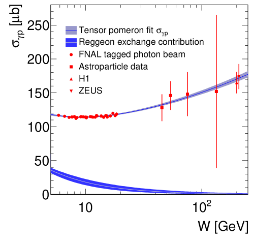
Figure 5: Comparison of the global fit to the photoproduction cross sections [28, 29, 30, 31]. The reggeon contribution is indicated. The experimental uncertainties of the fit are indicated as shaded bands.

The fit is very satisfactory. The $f_{2R}$ reggeon contribution is also indicated. It is found to be important for $W<30\,\mbox{GeV}$.

In figs. 6 to 11 we show our fit results for the HERA data. Here we indicate also the soft pomeron contribution. The contribution of the $f_{2R}$ component for the HERA DIS data which we use ($x<0.01$) is found to be very small from the fits and is hardly visible in figs. 6 to 11. The quality of our global fit, which has 25 parameters, is assessed in table 3, and is overall found to be very satisfactory. The experimental uncertainties indicated as shaded bands in fig. 5 and the following figures correspond to one standard deviations; see appendix D.

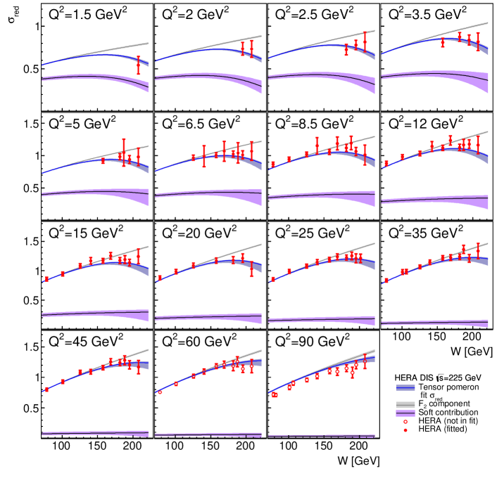
Figure 6: Comparison of the fit to DIS cross sections at centre-of-mass energy $225\,\text{GeV}$. We also show the soft contribution (soft pomeron plus $f_{2R}$ reggeon) and the contribution of the structure function $F_{2}$ in the reduced cross section; see (5.5). The experimental uncertainties of the fit are indicated as shaded bands.

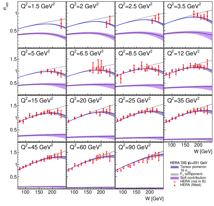
Figure 7: Comparison of the fit to DIS cross sections at centre-of-mass energy $251\,\text{GeV}$. We also show the soft contribution (soft pomeron plus $f_{2R}$ reggeon) and the contribution of the structure function $F_{2}$ in the reduced cross section; see (5.5). The experimental uncertainties of the fit are indicated as shaded bands.

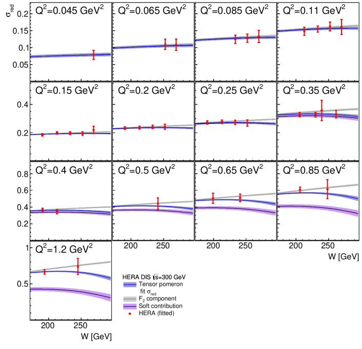
Figure 8: Comparison of the fit to DIS cross sections at centre-of-mass energy $300\,\text{GeV}$, at low $Q^{2}<1.5\,\text{GeV}^{2}$. We also show the soft contribution (soft pomeron plus $f_{2R}$ reggeon) and the contribution of the structure function $F_{2}$ in the reduced cross section; see (5.5). The experimental uncertainties of the fit are indicated as shaded bands.

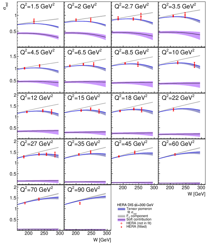
Figure 9: Comparison of the fit to DIS cross sections at centre-of-mass energy $300\,\text{GeV}$, at high $Q^{2}\geq 1.5\,\text{GeV}^{2}$. We also show the soft contribution (soft pomeron plus $f_{2R}$ reggeon) and the contribution of the structure function $F_{2}$ in the reduced cross section; see (5.5). The experimental uncertainties of the fit are indicated as shaded bands.

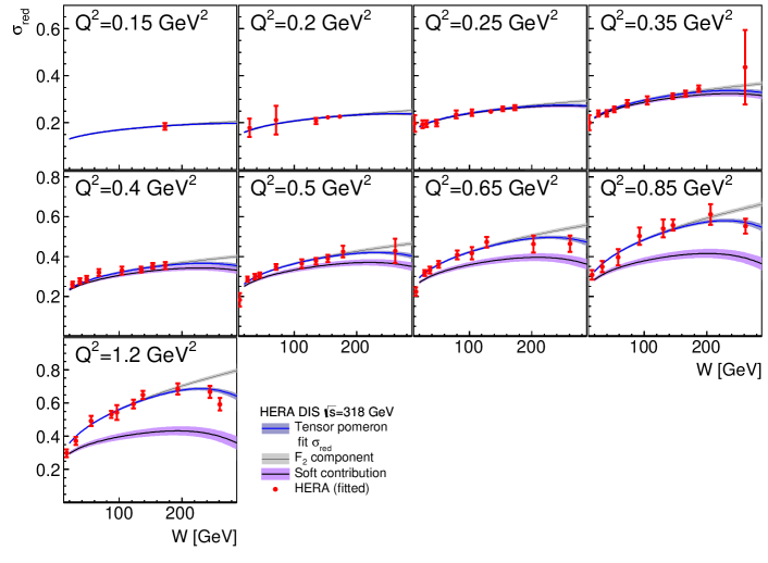
Figure 10: Comparison of the fit to DIS cross sections at centre-of-mass energy $318\,\text{GeV}$, at low $Q^{2}<1.5\,\text{GeV}^{2}$. We also show the soft contribution (soft pomeron plus $f_{2R}$ reggeon) and the contribution of the structure function $F_{2}$ in the reduced cross section; see (5.5). The experimental uncertainties of the fit are indicated as shaded bands.

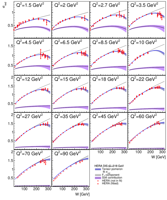
Figure 11: Comparison of the fit to DIS cross sections at centre-of-mass energy $318\,\text{GeV}$, at high $Q^{2}\geq 1.5\,\text{GeV}^{2}$. We also show the soft contribution (soft pomeron plus $f_{2R}$ reggeon) and the contribution of the structure function $F_{2}$ in the reduced cross section; see (5.5). The experimental uncertainties of the fit are indicated as shaded bands.

dataset	$\chi^{2}$	number of points
DIS $\sqrt{s}=225\,\text{GeV}$	$104.98$	$91$
DIS $\sqrt{s}=251\,\text{GeV}$	$113.12$	$118$
DIS $\sqrt{s}=300\,\text{GeV}$	$60.38$	$71$
DIS $\sqrt{s}=318\,\text{GeV}$	$271.82$	$245$
HERA DIS data, all $\sqrt{s}$	$553.77$	$525$
H1 photoproduction	$0.23$	$1$
ZEUS photoproduction	$0.03$	$1$
cosmic ray data	$0.62$	$4$
tagged photon beam	$33.29$	$30$
all datasets	$587.94$	$N_{DF}=(561-25)$, probability $6.0\%$

Table 3: Partial $\chi^{2}$ and number of data points per dataset, goodness of fit, number of degrees of freedom and fit probability for our tensor-pomeron fit. The partial $\chi^{2}$ numbers for the individual DIS centre-of-mass energies (upper part of the table) do not add up to the number quoted for all HERA DIS data. This is expected because correlated uncertainties between the different centre-of-mass energies also contribute.

We now want to discuss in detail the results of our fit. We start with the intercepts of the pomerons and of the $f_{2R}$ reggeon. From our global fit the soft pomeron ($\mathbbm{P}_{1}$) intercept comes out as

$$\alpha_{1}(0)=1+\epsilon_{1}\,,\qquad\epsilon_{1}=0.0935\,({}^{+76}_{-64})\,.$$ (5.13)

This is well compatible with the standard value $\epsilon\approx 0.08$ to $0.09$ obtained from hadronic reactions; see for instance chapters 3 of [4] and [11]. The value of the $f_{2R}$ intercept is found to be

$$\alpha_{2}(0)=0.485\,({}^{+88}_{-90})$$ (5.14)

and is in agreement with the determinations from [4, 11] which quote $\alpha_{2}(0)=0.5475$. For the hard pomeron $\mathbbm{P}_{0}$ we find

$$\alpha_{0}(0)=1+\epsilon_{0}\,,\qquad\epsilon_{0}=0.3008\,({}^{+73}_{-84})\,.$$ (5.15)

This is again a very reasonable value.

Next, let us turn to photoproduction; see fig. 5. The photoproduction is dominated by soft pomeron exchange in the energy range investigated, $6\,\mbox{GeV}<W<209\,\mbox{GeV}$. The $f_{2R}$ reggeon contribution is important for $W\lesssim 30\,\mbox{GeV}$ and is needed there in order to get a good fit to the data. The hard pomeron $\mathbbm{P}_{0}$ gives only a very small contribution. In fact, there is no evidence for a non-zero contribution of the hard pomeron to the photoproduction cross section in the energy range investigated here. At $W=200\,\mathrm{GeV}$, for instance, the fitted contributions to the photoproduction cross section are

$$\begin{split}170.4\,{}^{+4.2}_{-4.0}\>\mu{\rm b}&\qquad\mbox{for the soft pomeron }\mathbbm{P}_{1}\,,\\ 0.002\,{}^{+0.086}_{-0.002}\>\mu{\rm b}&\qquad\mbox{for the hard pomeron }\mathbbm{P}_{0}\,,\\ 0.84\,{}^{+0.99}_{-0.58}\>\mu{\rm b}&\qquad\mbox{for the $f_{2R}$ reggeon}.\end{split}$$

For lower $W$ values the relative contribution of the hard pomeron to photoproduction is even smaller due to $\epsilon_{0}>\epsilon_{1}$.

In figures 6-11 we show the comparison of our global fit with the HERA DIS data. Note that in figures 6, 7, 9, and 11, we also show the extrapolation of our fit to the region $50\,\mbox{GeV}^{2}\leq Q^{2}\leq 90\,\mbox{GeV}^{2}$. The HERA data in this region are not included in the fit but still reasonably well described by it. In our global fit we have as parameters also the pomeron-$\gamma^{*}\gamma^{*}$ coupling functions $\hat{a}_{j}(Q^{2})$ and $\hat{b}_{j}(Q^{2})$ ($j=0,1$); see table 1 and (A.18), (A.19). The latter are parametrised with the help of cubic splines; see appendix C. In figures 12 to 15 we show the fit results for these functions which are discussed further in appendices D and E. Note that above $Q^{2}=50\,\mbox{GeV}^{2}$ the displayed curves are extrapolations beyond the last spline knot. In essence, these functions are extrapolated using simple power laws in $Q^{2}$; see (C.3), (C.5) and (C.6) in appendix C.

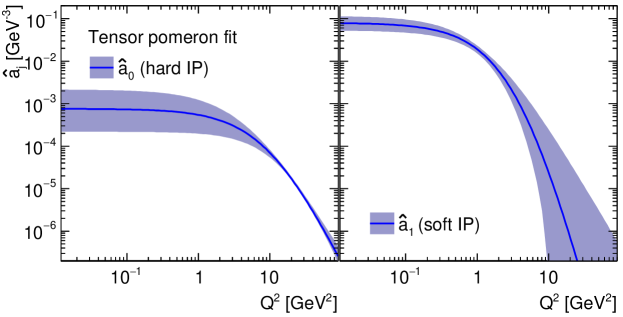
Figure 12: The pomeron-$\gamma^{*}\gamma^{*}$ coupling functions $\hat{a}_{j}(Q^{2})$ for $j=0$ (hard pomeron) and $j=1$ (soft pomeron); see (3), (3), and (A.19). The shaded bands indicate the experimental uncertainties.

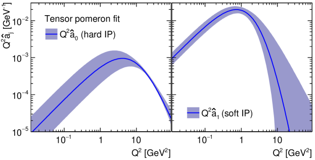
Figure 13: The pomeron-$\gamma^{*}\gamma^{*}$ coupling functions $Q^{2}\hat{a}_{j}(Q^{2})$ for $j=0$ (hard pomeron) and $j=1$ (soft pomeron); see (3), (3), and (A.19). The shaded bands indicate the experimental uncertainties.

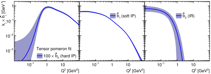
Figure 14: The pomeron- and reggeon-$\gamma^{*}\gamma^{*}$ coupling functions $\hat{b}_{j}(Q^{2})$ for $j=0$ (hard pomeron), $j=1$ (soft pomeron), and $j=2$ (reggeon); see (3), (3), (A.19), and (A.28). The shaded bands indicate the experimental uncertainties. More precisely, we show the functions $k_{j}\hat{b}_{j}(Q^{2})$, where $\hat{b}_{0}(Q^{2})$ is scaled up by a factor $k_{0}=100$ for displaying purposes while the functions $\hat{b}_{1}(Q^{2})$ and $\hat{b}_{2}(Q^{2})$ are not scaled up, that is $k_{1}=k_{2}=1$.

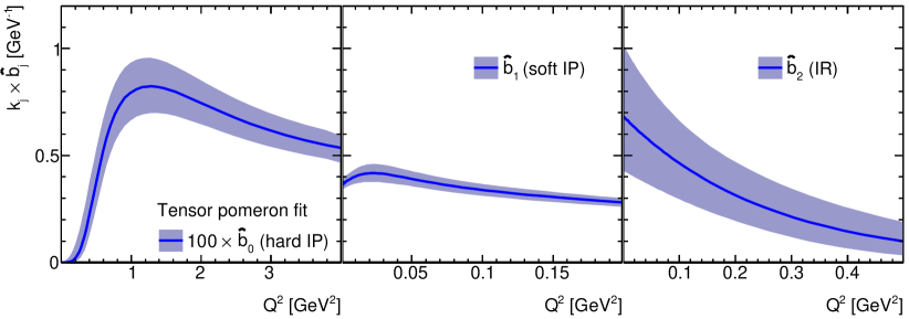
Figure 15: The pomeron- and reggeon-$\gamma^{*}\gamma^{*}$ coupling functions $\hat{b}_{j}(Q^{2})$ for $j=0$ (hard pomeron), $j=1$ (soft pomeron), and $j=2$ (reggeon); see (3), (3), (A.19), and (A.28). The shaded bands indicate the experimental uncertainties. More precisely, we show the functions $k_{j}\hat{b}_{j}(Q^{2})$, where $\hat{b}_{0}(Q^{2})$ is scaled up by a factor $k_{0}=100$ for displaying purposes while the functions $\hat{b}_{1}(Q^{2})$ and $\hat{b}_{2}(Q^{2})$ are not scaled up, that is $k_{1}=k_{2}=1$.

Let us now point out some salient features of our global fit to HERA DIS data, figures 6 to 11.

We see from figures 8 and 10 that the soft pomeron $\mathbbm{P}_{1}$ dominates $\sigma_{\rm red}$ for $Q^{2}\lesssim 1\,\mbox{GeV}^{2}$. For higher $Q^{2}$ (figures 6, 7, 9, 11) the soft component slowly decreases relative to the hard one. For the c. m. energies $\sqrt{s}$ investigated, the soft and hard components are of similar size near $Q^{2}\approx 5\,\mbox{GeV}^{2}$. Dominance of the hard component ($\mathbbm{P}_{0}$) can only be seen for $Q^{2}\gtrsim 20\,\mbox{GeV}^{2}$. Thus, our fit tells us that the soft pomeron ($\mathbbm{P}_{1}$) contribution is essential for an understanding of the HERA data for $Q^{2}<50\,\mbox{GeV}^{2}$ and $x<0.01$.

In figures 6 to 11 we have also indicated the contribution of the structure function $F_{2}$ alone to $\sigma_{\rm red}$; see (5.5). At fixed $s$ and $Q^{2}$, large $W$ corresponds to large $y$; see (2.2). At large $y$ the negative term $-\tilde{f}\sigma_{L}$ in $\sigma_{\rm red}$ (see (5.3),(5.4)) becomes important. The turning away of the data from the lines ’$F_{2}$ component’ therefore indicates a sizeable contribution from the longitudinal cross section $\sigma_{L}$. Our model gives a good description of this feature of the data.

Another way to assess the importance of $\sigma_{L}$ is to consider the ratio

$$R(W^{2},Q^{2})=\frac{\sigma_{L}(W^{2},Q^{2})}{\sigma_{T}(W^{2},Q^{2})}\,.$$ (5.16)

Our fit results for $R$ and for $F_{L}$ (3) are shown in fig. 16.

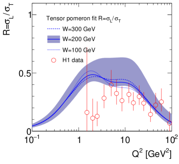
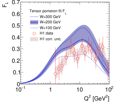
Figure 16: The ratio $R=\sigma_{L}/\sigma_{T}$ of longitudinal to transverse cross sections and the structure function $F_{L}$ are shown as a function of $Q^{2}$ for three choices of $W$ in comparison to data extracted directly from H1 cross section measurements at different centre-of-mass energies [32]. These data were taken at $W$ near $200\,\text{GeV}$ and are not included in our fit. The error bars correspond to the H1 experimental uncertainties. The experimental uncertainties of our fit are indicated for $W=200\,\text{GeV}$ as a shaded band. For the case of the $F_{L}$ measurement, the correlated H1 uncertainty contribution is shown as a hatched band.

Within the fit ansatz, the ratio $R=\sigma_{L}/\sigma_{T}$ of longitudinal to transverse cross sections depends on $Q^{2}$ and $W$. Figure 16 shows the dependence of $R$ and of the structure function $F_{L}$ on $Q^{2}$ at fixed $W$. In both panels, H1 data [32] are shown for comparison with our global fit results. The H1 data are extracted in a model-independent way directly from H1 cross sections measured at a fixed $Q^{2}$ and $x$ but different centre-of-mass energies. The $W$ corresponding to the H1 data is around $200\,\text{GeV}$, the extreme values are $W=232\,\text{GeV}$ at $Q^{2}=1.5\,\text{GeV}^{2}$ and $W=193\,\text{GeV}$ at $Q^{2}=45\,\text{GeV}^{2}$. The same H1 cross section data [32] also contribute strongly to the HERA data combination of DIS cross sections [27], which is used as input to our fit. Still, the fit predicts $R$ and $F_{L}$ somewhat above the H1 data. The H1 $R$ and $F_{L}$ data however have a sizeable point-to-point correlated uncertainty, which for $F_{L}$ is of order $0.045$ as indicated. Moreover, the determinations of $R$ in the fit or directly from H1 cross sections probe different aspects of the data.

In the H1 extraction from data, the structure function $F_{2}$ is a free parameter for each point in $Q^{2}$ and $W$, which basically is set by the measurements at high centre-of-mass energies $\sqrt{s}=318\,\text{GeV}$ and $W=200\,\text{GeV}$ (figure 11). The structure function $F_{L}$ and the ratio $R$ are then determined largely by the data points at low $\sqrt{s}=225\,\text{GeV}$ and $W=200\,\text{GeV}$ (figure 6).

In contrast, $F_{2}$ in our fit is determined largely by data from lower $W$ and the power exponents $\epsilon_{i}$. The functions $F_{L}$ and $R$ are then determined from all centre-of-mass energies together at their respective largest $W$; however, the most precise data at largest $W$ (figure 11) contribute most.

In appendix F we present further discussion of the ratio $R$ (5.16). We show in particular that the rather large value of $R$ resulting from the fit is not affected much by making different assumptions for the fit parameters.

6 Discussion

In this article we developed a two-tensor-pomeron model and used it for a fit to data from photoproduction and from HERA deep-inelastic lepton-nucleon scattering at low $x$. The c. m. energy range of these data is $6$ to $318\,\mbox{GeV}$, the $Q^{2}$ range $0$ to $50\,\mbox{GeV}^{2}$. For the theoretical description we also included the $f_{2R}$ reggeon exchange which turned out to be relevant for energies $\lesssim 30\,\mbox{GeV}$. The fit parameters were the intercepts of the two pomerons and of the reggeon, and their coupling functions to real and virtual photons. The fit turned out to be very satisfactory and allowed us to determine, for instance, the intercepts of the hard pomeron ($\mathbbm{P}_{0}$), of the soft pomeron ($\mathbbm{P}_{1}$) and of the $f_{2R}$ reggeon. We obtained very reasonable numbers for these intercepts; see table 2. The real photoabsorption cross section $\sigma_{\gamma p}$ is found to be dominated by soft pomeron exchange with, at lower energies, a contribution from $f_{2R}$ reggeon exchange. Within the errors of our fit a hard pomeron contribution is not visible for photoproduction. But as $Q^{2}$ increases the hard pomeron becomes more and more important. Hard and soft pomeron give contributions of roughly equal size for $Q^{2}\approx 5\,\mbox{GeV}^{2}$, but the soft contribution is still clearly visible for $Q^{2}\approx 20\,\mbox{GeV}^{2}$.

Our results indicate that in the energy and $Q^{2}$ range investigated the $\gamma^{*}$-proton absorption cross sections rise with energy as $W^{2\epsilon_{1}}$ for low $Q^{2}$ and change to $W^{2\epsilon_{0}}$ for high $Q^{2}$. Here $\epsilon_{1}\approx 0.09$ and $\epsilon_{0}\approx 0.30$ are the intercepts minus one of the pomerons $\mathbbm{P}_{1}$ and $\mathbbm{P}_{0}$; see table 2. It has been realised already a long time ago (see for instance [33]) that parton densities in hadrons become large in high-energy or low-$x$ scattering. This can give rise to parton recombination and saturation, potentially taming the growth of cross sections at high energies. At the energies investigated here we find no indication that the rise of the $\gamma^{*}$-proton absorption cross sections levels off. The question can be asked if the $\gamma^{*}p$ cross sections could continue to rise indefinitely for higher and higher $W$. We note first that there is no Froissart-like bound for the rise of the $\gamma^{*}p$ cross sections since $\gamma^{*}$ is not an asymptotic hadronic state. Thus, there is no non-linear unitarity relation for the $\gamma^{*}p$ cross sections which would be a prerequisite for the derivation of a Froissart-like bound. The $\gamma^{*}p$ cross sections may well stop to rise at higher $W$ due to saturation effects, but this will then, in our opinion, not be related to the Froissart-Martin-Lukaszuk bound [34, 35, 36] which applies to hadronic cross sections. We see no rigorous theoretical argument against an indefinite rise of the $\gamma^{*}p$ cross sections with $W$. Note that these ’$\gamma^{*}p$ cross sections’ are in reality current-current correlation functions. The standard folklore of quantum field theory (QFT) is that such functions should be polynomially bounded which is clearly fulfilled in our case. Some time ago, one of us investigated theoretically the low-$x$ behaviour of the $\gamma^{*}p$ cross sections in QCD [37]. There, arguments were given that identify two regimes in low-$x$ DIS, one for low $Q^{2}$ and one for high $Q^{2}$. It was argued that, in the high $Q^{2}$-region of low-$x$, DIS could be related to a critical phenomenon where, for instance, $\epsilon_{0}$ would be one of the critical exponents. In such a picture it would be natural to have a power rise with $W$ for the $\gamma^{*}p$ cross sections $\sigma_{T}$ and $\sigma_{L}$. But to know the actual behaviour of $\sigma_{T}$ and $\sigma_{L}$ for $W$ values higher than available today we will have to wait for future experiments.

We can obtain further support for the view that low-$x$ DIS at high enough $Q^{2}$ can be understood as a critical phenomenon from our present results. We see from (3.14) and (3.15) and the fit results for $\hat{a}_{j}(Q^{2})$ and $\hat{b}_{j}(Q^{2})$ ($j=0,1$) summarised in tables 4 and 5 that for $Q^{2}\gtrsim 20\,\mbox{GeV}^{2}$ the $\gamma^{*}p$ cross sections are well represented by simple power laws in $Q^{2}$ and $W^{2}$:

$$\sigma_{T}(W^{2},Q^{2})+\sigma_{L}(W^{2},Q^{2}) \propto\hat{b}_{0}(Q^{2})\,(W^{2})^{\epsilon_{0}}$$

$$\propto(Q^{2})^{-\eta_{0}}\,(W^{2})^{\epsilon_{0}}\,,$$ (6.1)

$$\sigma_{L}(W^{2},Q^{2}) \propto Q^{2}\,\hat{a}_{0}(Q^{2})\,(W^{2})^{\epsilon_{0}}$$

$$\propto(Q^{2})^{-\delta_{0}}\,(W^{2})^{\epsilon_{0}}\,.$$ (6.2)

Here we have from (C.3), (C.5), (C.6), and tables 4 and 5

$$\begin{split}\delta_{0}&=2.51\,({}^{+68}_{-57})\\ \eta_{0}&={}-n_{0,7}=0.967(73)\,.\end{split}$$ (6.3)

Such simple power laws (6) and (6) were, indeed, suggested in [37]. The quantities $\delta_{0}$ and $\eta_{0}$ are in this view, together with $\epsilon_{0}$, critical exponents.

In our work we have paid particular attention to describing and fitting not only the structure function $F_{2}$, which is proportional to $\sigma_{T}+\sigma_{L}$, but the reduced cross section $\sigma_{\rm red}$ (5.3), (5.4) which contains all experimentally available information on $\sigma_{T}$ and $\sigma_{L}$ separately. Our fit results for $R=\sigma_{L}/\sigma_{T}$ indicate that it is rather large, $R\gtrsim 0.4$ for $1\,\mbox{GeV}^{2}\lesssim Q^{2}\lesssim 10\,\mbox{GeV}^{2}$ even taking the one standard deviation errors into account; see fig. 16, and also fig. 17 in appendix F. We note that such a large value of $R$, taken at face value, presents problems for the standard colour-dipole model of low-$x$ DIS. In the framework of this model two of us derived a rigorous upper limit of $R\leq 0.37248$; see [38, 39] and references therein. The derivation of this bound uses only the standard dipole-model relations, in particular, the expressions for the photon wave functions at lowest order in the strong coupling constant $\alpha_{s}$ and the non-negativity of the dipole-proton cross sections. The then available H1 data for $R$ from [40] were compared with this and related bounds in [41]. A very conservative conclusion from our findings concerning $R$ in the present paper is, therefore, as follows. If one wants to be sure to be in a kinematic region where the colour-dipole model can be applied in the HERA energy range one should limit oneself to $Q^{2}\gtrsim 10\,\mbox{GeV}^{2}$. Below $Q^{2}\approx 10\,\mbox{GeV}^{2}$ corrections to the standard dipole picture, as listed and discussed e. g. in [38], may become important. There is, however, a strong caveat concerning the $R$ determination from our fit to $\sigma_{\text{red}}$. We use our explicit tensor pomeron model and, thus, our $R$ values are not derived in a model-independent way. We cannot exclude the possibility that a different model may give somewhat different results for $R$ from a fit to $\sigma_{\text{red}}$.

The next topic we want to address briefly concerns the twist expansion for the structure functions of DIS; see for instance [42]. Note that the twist expansion is, in essence, an expansion in inverse powers of $Q^{2}$. Thus, it only makes sense for sufficiently large $Q^{2}$ and, certainly, cannot be extended down to $Q^{2}=0$. It is well known that the leading twist-2 terms correspond to the QCD-improved parton picture with parton distributions obeying the famous DGLAP evolution equations [43, 44, 45]. In our framework the question arises how the hard and soft pomeron contributions will contribute to leading and higher twists. It is tempting to associate, at large enough $Q^{2}$, the hard pomeron contribution with leading twist 2 and the soft pomeron contribution with higher twists. Indeed, the latter vanishes relative to the former for large $Q^{2}$ where the ratios of the $\mathbbm{P}_{j}\gamma^{*}\gamma^{*}$ coupling functions $\hat{a}_{j}(Q^{2})$ and $\hat{b}_{j}(Q^{2})$ for the soft ($j=1$) and hard ($j=0$) pomeron behave as

$$\begin{split}\frac{\hat{a}_{1}(Q^{2})}{\hat{a}_{0}(Q^{2})}&\propto(Q^{2})^{\delta_{0}-\delta_{1}}\approx(Q^{2})^{-3}\,,\\ \frac{\hat{b}_{1}(Q^{2})}{\hat{b}_{0}(Q^{2})}&\propto(Q^{2})^{n_{1,7}-n_{0,7}}\approx(Q^{2})^{-1.2}\,;\end{split}$$ (6.4)

see tables 4 and 5. This point of view, as expressed above, is close to what was advocated in [46]. Following [46] we would then conclude that higher twist effects – the soft pomeron contribution – stay important for $x<0.01$ up to $Q^{2}\approx 20\,\mbox{GeV}^{2}$. Certainly, it will be worthwhile to study in more detail the connection of our two-tensor-pomeron model with the description of the HERA data using parton distribution functions and with the DGLAP and BFKL [47, 48] evolution equations. But this clearly goes beyond the scope of the present work.

As we have stated in the introduction it is not our aim here to give a comparison of the various theoretical approaches to low-$x$ DIS physics. Let us just briefly comment on some recent fits to the HERA low-$x$ data where various methods were used. In [40] a so-called $\lambda$-fit in which $F_{2}$ is approximated by a power law in $x$ with a $Q^{2}$-dependent exponent was presented. The ansatz was then extended by adding in this exponent a ’$\lambda^{\prime}$ term’ proportional to $\ln x$. Furthermore, a fit based on DGLAP evolution, as well as dipole model fits were presented. In [49] a higher-twist ansatz was added to a DGLAP fit. Dipole models were used for example in [50], and DGLAP fits with BFKL-type low-$x$ resummation improvement in [51] and [52]. However, in all these approaches the limit $Q^{2}\to 0$, that is the photoabsorption cross section, is not included in the considerations. Typically, a minimum $Q^{2}$ of order $3.5\,\mbox{GeV}^{2}$ is imposed. In our approach, on the other hand, photoabsorption is treated in the same framework as DIS, allowing a detailed investigation of the transition from hard to soft scattering.

7 Conclusions

In summary, we have presented a fit, based on a two-tensor-pomeron model, to photoproduction and low-$x$ deep-inelastic lepton-nucleon scattering data from HERA. We have determined the intercepts of the soft and hard pomeron and of the $f_{2R}$ reggeon, obtaining very reasonable numbers; see table 2.

The two-tensor-pomeron model allows us to describe the transition from $Q^{2}=0$ and low $Q^{2}$, where the real or virtual photon acts hadron-like and the soft pomeron dominates, to high $Q^{2}$, the hard scattering regime dominated by the hard pomeron. The transition region where both pomerons contribute significantly was found to be roughly $0<Q^{2}<20\,\mbox{GeV}^{2}$. For the photoproduction cross section $\sigma_{\gamma p}(W)$ we found no significant contribution from the hard pomeron. Thus, $\sigma_{\gamma p}(W)$ is, in the c. m. energy range $6\,\mbox{GeV}<W<209\,\mbox{GeV}$, dominated by soft-pomeron exchange with a significant $f_{2R}$ contribution for $W<30\,\mbox{GeV}$.

In the high-$Q^{2}$ and low-$x$ regime of DIS we found a good representation of the $\gamma^{*}p$ cross sections $\sigma_{T}+\sigma_{L}$ and $\sigma_{L}$ as products of simple powers in $Q^{2}$ and $W^{2}$; see (6)-(6.3). This may suggest that low-$x$ phenomena at high enough $Q^{2}$ may have an interpretation as a critical phenomenon as suggested in [37].

In contrast to our tensor-pomeron model which gives an excellent description of the real photoabsorption cross section we found that a vector ansatz for the pomeron is ruled out as it gives zero contribution there; see section 4 and appendix B.

We are looking forward to further tests of our two-tensor-pomeron model at future lepton-proton scattering experiments in the low-$x$ regime, for instance at a future Electron-Ion-Collider [55] or a Large Hadron Electron Collider LHeC [56]. In particular, measurements of $\sigma_{L}$ and $R=\sigma_{L}/\sigma_{T}$ would be very welcome since these quantities are potentially very promising for a discrimination between different models, while at present their experimental errors are large.

Appendix A Effective propagators and vertices

For the soft pomeron $\mathbbm{P}_{1}$ we use the effective propagator as given in (3.10) and (3.11) of [11],
     

$$i\Delta^{(\mathbbm{P}_{1})}_{\mu\nu,\kappa\lambda}(s,t)=\frac{1}{4s}\left(g_{\mu\kappa}g_{\nu\lambda}+g_{\mu\lambda}g_{\nu\kappa}-\frac{1}{2}g_{\mu\nu}g_{\kappa\lambda}\right)\,(-is\tilde{\alpha}^{\prime}_{1})^{\alpha_{1}(t)-1}\,.$$ (A.1)

The $\mathbbm{P}_{1}$ trajectory function is taken as linear in $t$,

$$\alpha_{1}(t)=1+\epsilon_{1}+\alpha^{\prime}_{1}t\,,$$ (A.2)

For the slope parameter $\alpha^{\prime}_{1}$ and the parameter $\tilde{\alpha}^{\prime}_{1}$ multiplying the squared energy $s$ we take the default values from [11],

$$\begin{split}\alpha^{\prime}_{1}&=0.25\,\mbox{GeV}^{-2}\,,\\ \tilde{\alpha}^{\prime}_{1}&=\alpha^{\prime}_{1}\,.\end{split}$$ (A.3)

The intercept parameter $\epsilon_{1}$ is in our work left free to be fitted. From our fits described in section 5 we find (see table 2)

$$\epsilon_{1}=0.0935\,({}^{+76}_{-64})\,.$$ (A.4)

For the hard-pomeron propagator our ansatz is similar to (A.1), (A.2),
     

$$i\Delta^{(\mathbbm{P}_{0})}_{\mu\nu,\kappa\lambda}(s,t)=\frac{1}{4s}\left(g_{\mu\kappa}g_{\nu\lambda}+g_{\mu\lambda}g_{\nu\kappa}-\frac{1}{2}g_{\mu\nu}g_{\kappa\lambda}\right)\,(-is\tilde{\alpha}^{\prime}_{0})^{\alpha_{0}(t)-1}\,,$$ (A.5)

with

$$\alpha_{0}(t)=1+\epsilon_{0}+\alpha^{\prime}_{0}t\,,$$ (A.6)

and the parameter $\epsilon_{0}$ to be determined from experiment. For $\alpha^{\prime}_{0}$ and $\tilde{\alpha}^{\prime}_{0}$ we take, for lack of better knowledge, the same values as for the soft pomeron,

$$\alpha^{\prime}_{0}=\tilde{\alpha}^{\prime}_{0}=0.25\,\mbox{GeV}^{-2}\,.$$ (A.7)

From the fits in section 5 we get (see table 2)

$$\epsilon_{0}=0.3008\,({}^{+73}_{-84})\,.$$ (A.8)

The ansatz for the $\mathbbm{P}_{1}pp$ vertex is given in (3.43) of [11]. Making an analogous ansatz for the hard pomeron we get:
     

$$\begin{split}i\Gamma_{\mu\nu}^{(\mathbbm{P}_{j}pp)}(p^{\prime},p)=&-i\,3\beta_{jpp}F_{1}^{(j)}[(p^{\prime}-p)^{2}]\\ &\times\left\{\frac{1}{2}\left[\gamma_{\mu}(p^{\prime}+p)_{\nu}+\gamma_{\nu}(p^{\prime}+p)_{\mu}\right]-\frac{1}{4}\,g_{\mu\nu}(\not\!p^{\prime}+\not\!p)\right\}\,,\qquad(j=0,1)\,.\end{split}$$ (A.9)

Here $\beta_{jpp}$ are coupling constants of dimension $\mbox{GeV}^{-1}$ and $F_{1}^{(j)}(t)$ are form factors normalised to

$$F_{1}^{(j)}(0)=1\,.$$ (A.10)

The standard value for the coupling constant of the soft pomeron to protons is

$$\beta_{1pp}=1.87\,\mbox{GeV}^{-1}\,;$$ (A.11)

see (3.44) of [11]. The traditional choice for the form factor $F_{1}^{(1)}(t)$ is the Dirac electromagnetic form factor of the proton even if it is clear that this cannot be strictly correct; see the discussion in chapter 3.2 of [4]. But this is not relevant for our present work where we only need the form factors at $t=0$ where they are equal to 1; see (A.10). For lack of better knowledge we take

$$\beta_{0pp}=\beta_{1pp}\,.$$ (A.12)

For the processes that we consider in the present paper this gives no restriction for our fits since only the products $\beta_{jpp}\hat{a}_{j}(Q^{2})$ and $\beta_{jpp}\hat{b}_{j}(Q^{2})$ enter as parameters.

For our ansatz for the $\mathbbm{P}_{j}\gamma^{*}\gamma^{*}$ vertices we need the rank-4 tensor functions defined in (3.18) and (3.19) of [11],

$$\Gamma_{\mu\nu\kappa\lambda}^{(0)}(k_{1},k_{2})=\, [(k_{1}\cdot k_{2})g_{\mu\nu}-k_{2\mu}k_{1\nu}]\left[k_{1\kappa}k_{2\lambda}+k_{2\kappa}k_{1\lambda}-\frac{1}{2}(k_{1}\cdot k_{2})g_{\kappa\lambda}\right]\,,$$ (A.13)

$$\Gamma_{\mu\nu\kappa\lambda}^{(2)}(k_{1},k_{2})=\, (k_{1}\cdot k_{2})(g_{\mu\kappa}g_{\nu\lambda}+g_{\mu\lambda}g_{\nu\kappa})+g_{\mu\nu}(k_{1\kappa}k_{2\lambda}+k_{2\kappa}k_{1\lambda})$$

$$-k_{1\nu}k_{2\lambda}g_{\mu\kappa}-k_{1\nu}k_{2\kappa}g_{\mu\lambda}-k_{2\mu}k_{1\lambda}g_{\nu\kappa}-k_{2\mu}k_{1\kappa}g_{\nu\lambda}$$ (A.14)

$$-[(k_{1}\cdot k_{2})g_{\mu\nu}-k_{2\mu}k_{1\nu}]\,g_{\kappa\lambda}\,.$$

We have for $i=0,2$

$$\Gamma_{\mu\nu\kappa\lambda}^{(i)}(k_{1},k_{2})=\Gamma_{\mu\nu\lambda\kappa}^{(i)}(k_{1},k_{2})=\Gamma_{\nu\mu\kappa\lambda}^{(i)}(k_{2},k_{1})=\Gamma_{\mu\nu\kappa\lambda}^{(i)}(-k_{1},-k_{2})\,,$$ (A.15)

$$\begin{split}&k_{1}^{\mu}\Gamma_{\mu\nu\kappa\lambda}^{(i)}(k_{1},k_{2})=0\,,\\ &k_{2}^{\nu}\Gamma_{\mu\nu\kappa\lambda}^{(i)}(k_{1},k_{2})=0\,,\end{split}$$ (A.16)

$$\Gamma_{\mu\nu\kappa\lambda}^{(i)}(k_{1},k_{2})\,g^{\kappa\lambda}=0\,.$$ (A.17)

Now we can write down our ansatz for the $\mathbbm{P}_{j}\gamma^{*}\gamma^{*}$ vertices in analogy to the $\mathbbm{P}\rho\rho$ vertex in (3.47) of [11]:
     

$$\begin{split}i\Gamma_{\mu\nu\kappa\lambda}^{(\mathbbm{P}_{j}\gamma^{*}\gamma^{*})}(q^{\prime},q)=&i\left[2a_{j\gamma^{*}\gamma^{*}}(q^{2},q^{\prime 2},t)\Gamma_{\mu\nu\kappa\lambda}^{(0)}(q^{\prime},-q)-b_{j\gamma^{*}\gamma^{*}}(q^{2},q^{\prime 2},t)\Gamma_{\mu\nu\kappa\lambda}^{(2)}(q^{\prime},-q)\right]\,,\\ &\qquad\qquad t=(q-q^{\prime})^{2}\,,\qquad j=0,1\,.\end{split}$$ (A.18)

Here the coupling parameters $a_{j\gamma^{*}\gamma^{*}}$ and $b_{j\gamma^{*}\gamma^{*}}$ have dimensions $\mbox{GeV}^{-3}$ and $\mbox{GeV}^{-1}$, respectively. In our present work only the values of these parameters for

$$q^{2}=q^{\prime 2}=-Q^{2}\,,\qquad t=0$$

enter. Therefore, we set, pulling out also a factor $e^{2}$,

$$\begin{split}a_{j\gamma^{*}\gamma^{*}}(-Q^{2},-Q^{2},0)&=e^{2}\hat{a}_{j}(Q^{2})\,,\\ b_{j\gamma^{*}\gamma^{*}}(-Q^{2},-Q^{2},0)&=e^{2}\hat{b}_{j}(Q^{2})\,,\\ j=0,1\,.&\end{split}$$ (A.19)

Our ansätze for the effective propagator and the vertices for $f_{2R}$-reggeon exchange are as follows. For the $f_{2R}$ propagator we set (see (3.12), (3.13) of [11])
     

$$i\Delta^{(f_{2R})}_{\mu\nu,\kappa\lambda}(s,t)=\frac{1}{4s}\left(g_{\mu\kappa}g_{\nu\lambda}+g_{\mu\lambda}g_{\nu\kappa}-\frac{1}{2}g_{\mu\nu}g_{\kappa\lambda}\right)(-is\tilde{\alpha}^{\prime}_{2})^{\alpha_{2}(t)-1}\,,$$ (A.20)

$$\alpha_{2}(t)=\alpha_{2}(0)+\alpha^{\prime}_{2}t\,$$ (A.21)

with $\alpha_{2}(0)$ as fit parameter. For $\alpha^{\prime}_{2}$ and $\tilde{\alpha}^{\prime}_{2}$ we take the default values from (3.13) of [11]:

$$\begin{split}\alpha^{\prime}_{2}&=0.9\,\mbox{GeV}^{-2}\,,\\ \tilde{\alpha}^{\prime}_{2}&=\alpha^{\prime}_{2}\,.\end{split}$$ (A.22)

Our fit gives (see table 2)

$$\alpha_{2}(0)=0.485\,({}^{+88}_{-90})$$ (A.23)

which is nicely compatible with the default value from (3.13) of [11]: $\alpha_{2}(0)=0.5475$.

The $f_{2R}pp$ vertex is given in (3.49), (3.50) of [11] as
     

$$\begin{split}i\Gamma_{\mu\nu}^{(f_{2R}pp)}(p^{\prime},p)=&-ig_{f_{2R}pp}\frac{1}{M_{0}}F_{1}[(p^{\prime}-p)^{2}]\\ &\times\bigg{\{}\frac{1}{2}[\gamma_{\mu}(p^{\prime}+p)_{\nu}+\gamma_{\nu}(p^{\prime}+p)_{\mu}]-\frac{1}{4}g_{\mu\nu}(\not\!p^{\prime}+\not\!p)\bigg{\}}\,,\end{split}$$ (A.24)

$$g_{f_{2R}pp}=11.04\,,\qquad M_{0}=1~{}\text{GeV}\,.$$ (A.25)

In our paper we use as coupling parameter

$$\beta_{2pp}=\frac{1}{3M_{0}}\,g_{f_{2R}pp}=3.68~{}\text{GeV}^{-1}\,.$$ (A.26)

The ansatz for the $f_{2R}\gamma^{(*)}\gamma^{(*)}$ vertex for real and virtual photons will be taken with the same structure as for $f_{2}\gamma\gamma$ (see (3.39), (3.40) of [11]),
             $i\Gamma_{\mu\nu\kappa\lambda}^{(f_{2R}\gamma^{*}\gamma^{*})}(q^{\prime},q)\,.$

In the present work we need this vertex only for

$$q^{\prime}=q\,,\qquad q^{2}=-Q^{2}\leq 0\,,$$ (A.27)

and our ansatz for this case reads

$$i\Gamma_{\mu\nu\kappa\lambda}^{(f_{2R}\gamma^{*}\gamma^{*})}(q,q)=i\,\left[2e^{2}\hat{a}_{2}(Q^{2})\,\Gamma_{\mu\nu\kappa\lambda}^{(0)}(q,-q)-e^{2}\hat{b}_{2}(Q^{2})\,\Gamma_{\mu\nu\kappa\lambda}^{(2)}(q,-q)\right]\,.$$ (A.28)

Appendix B Formulae for a hypothetical vector pomeron

In this appendix we collect the necessary formulae for the (hypothetical) vector pomeron couplings to protons and real photons. These formulae are used in section 4. The $\mathbbm{P}_{V}pp$ vertex and the $\mathbbm{P}_{V}$ propagator are standard; see e. g. [4] and appendix B of [14]. We have
     

$$i\Gamma_{\sigma}^{(\mathbbm{P}_{V}pp)}(p^{\prime},p)=-i\,3\beta_{\mathbbm{P}_{V}pp}F_{1}[(p-p^{\prime})^{2}]M_{0}\gamma_{\sigma}\,,$$ (B.1)

with $\beta_{\mathbbm{P}_{V}pp}=1.87\,\mbox{GeV}^{-1}$, $M_{0}=1\,\mbox{GeV}$, and
     

$$i\Delta_{\rho\sigma}^{(\mathbbm{P}_{V})}(W^{2},t)=\frac{1}{M_{0}^{2}}\,g_{\rho\sigma}(-iW^{2}\alpha^{\prime}_{{\mathbbm{P}_{V}}})^{\alpha_{\mathbbm{P}_{V}}(t)-1}\,.$$ (B.2)

In (B.1) $F_{1}(t)$ is a form factor normalised to $F_{1}(0)=1$. In (B.2) $\alpha_{\mathbbm{P}_{V}}(t)$ is the vector pomeron trajectory function and $\alpha^{\prime}_{\mathbbm{P}_{V}}$ is the slope parameter. The numerical values for these quantities play no role in the following and in section 4. For the $\mathbbm{P}_{V}\gamma\gamma$ vertex we assume that it respects the standard rules of QFT. We have, orienting here for simplicity both photons as outgoing,

             $$i\Gamma_{\mu\nu\rho}^{(\mathbbm{P}_{V}\gamma\gamma)}(k_{1},k_{2})\,.$$ (B.3)

For this vertex function we have the constraints of Bose symmetry for the two photons,

$$\Gamma_{\mu\nu\rho}^{(\mathbbm{P}_{V}\gamma\gamma)}(k_{1},k_{2})=\Gamma_{\nu\mu\rho}^{(\mathbbm{P}_{V}\gamma\gamma)}(k_{2},k_{1})\,,$$ (B.4)

and of gauge invariance,

$$\begin{split}k_{1}^{\mu}\Gamma_{\mu\nu\rho}^{(\mathbbm{P}_{V}\gamma\gamma)}(k_{1},k_{2})&=0\,,\\ k_{2}^{\nu}\Gamma_{\mu\nu\rho}^{(\mathbbm{P}_{V}\gamma\gamma)}(k_{1},k_{2})&=0\,.\end{split}$$ (B.5)

The vertex $\mathbbm{P}_{V}\gamma\gamma$ should also respect parity invariance. We have then 14 tensors, constructed from $k_{1}$, $k_{2}$ and the metric tensor, at our disposal,

$$\begin{split}&k_{1\mu}k_{1\nu}k_{1\rho}\,,\qquad k_{1\mu}k_{1\nu}k_{2\rho}\,,\qquad k_{1\mu}k_{2\nu}k_{1\rho}\,,\qquad k_{1\mu}k_{2\nu}k_{2\rho}\,,\\ &k_{2\mu}k_{1\nu}k_{1\rho}\,,\qquad k_{2\mu}k_{1\nu}k_{2\rho}\,,\qquad k_{2\mu}k_{2\nu}k_{1\rho}\,,\qquad k_{2\mu}k_{2\nu}k_{2\rho}\,,\\ &g_{\mu\nu}k_{1\rho}\,,\qquad g_{\mu\rho}k_{1\nu}\,,\qquad g_{\nu\rho}k_{1\mu}\,,\qquad g_{\mu\nu}k_{2\rho}\,,\qquad g_{\mu\rho}k_{2\nu}\,,\qquad g_{\nu\rho}k_{2\mu}\,.\\ \end{split}$$ (B.6)

To construct the most general vertex (B.3) we have to multiply these tensors with invariant functions depending on $k_{1}^{2}$, $k_{2}^{2}$, and $(k_{1}+k_{2})^{2}$, and take their sum. In the following, however, we shall only consider the case $k_{1}^{2}=k_{2}^{2}$. With the requirement (B.4) we obtain then the following general form for $\Gamma^{(\mathbbm{P}_{V}\gamma\gamma)}$:

$$\begin{split}\Gamma_{\mu\nu\rho}^{(\mathbbm{P}_{V}\gamma\gamma)}(k_{1},k_{2})=&{}\,A_{1}(k_{1\mu}k_{1\nu}k_{1\rho}+k_{2\mu}k_{2\nu}k_{2\rho})+A_{2}(k_{1\mu}k_{1\nu}k_{2\rho}+k_{2\mu}k_{2\nu}k_{1\rho})\\ &+A_{3}(k_{1\mu}k_{2\nu}k_{1\rho}+k_{1\mu}k_{2\nu}k_{2\rho})+A_{4}(k_{2\mu}k_{1\nu}k_{1\rho}+k_{2\mu}k_{1\nu}k_{2\rho})\\ &+A_{5}(g_{\mu\nu}k_{1\rho}+g_{\mu\nu}k_{2\rho})+A_{6}(g_{\mu\rho}k_{1\nu}+g_{\nu\rho}k_{2\mu})+A_{7}(g_{\nu\rho}k_{1\mu}+g_{\mu\rho}k_{2\nu})\,,\end{split}$$ (B.7)

with coefficient functions

$$A_{j}=A_{j}(k_{1}^{2},(k_{1}+k_{2})^{2})\,,\qquad j=1,\dots,7\,.$$ (B.8)

Imposing gauge invariance we find, using (B.5), the relations

$$\begin{split}k_{1}^{2}A_{1}+(k_{1}\cdot k_{2})A_{4}+A_{5}+A_{6}&=0\,,\\ (k_{1}\cdot k_{2})A_{1}+k_{1}^{2}A_{3}&=0\,,\\ k_{1}^{2}A_{2}+(k_{1}\cdot k_{2})A_{4}+A_{5}&=0\,,\\ (k_{1}\cdot k_{2})A_{2}+k_{1}^{2}A_{3}+A_{7}&=0\,,\\ (k_{1}\cdot k_{2})A_{6}+k_{1}^{2}A_{7}&=0\,.\end{split}$$ (B.9)

Now we specialise for real photons and assume a general, non-vanishing product of their 4-momenta,

$$k_{1}^{2}=k_{2}^{2}=0\,,\qquad k_{1}\cdot k_{2}\neq 0\,.$$ (B.10)

This gives

$$\begin{split}A_{1}&=0\,,\\ A_{6}&=0\,,\\ A_{5}&=-(k_{1}\cdot k_{2})A_{4}\,,\\ A_{7}&=-(k_{1}\cdot k_{2})A_{2}\end{split}$$ (B.11)

and hence the final form for $\Gamma^{(\mathbbm{P}_{V}\gamma\gamma)}$:

$$\begin{split}\Gamma_{\mu\nu\rho}^{(\mathbbm{P}_{V}\gamma\gamma)}(k_{1},k_{2})=&{}\,\hat{A}_{2}\left[k_{1\mu}(k_{1\nu}k_{2\rho}-(k_{1}\cdot k_{2})g_{\nu\rho})+(k_{2\mu}k_{1\rho}-(k_{1}\cdot k_{2})g_{\mu\rho})k_{2\nu}\right]\\ &+\hat{A}_{3}k_{1\mu}k_{2\nu}(k_{1\rho}+k_{2\rho})\\ &+\hat{A}_{4}(k_{2\mu}k_{1\nu}-(k_{1}\cdot k_{2})g_{\mu\nu})(k_{1\rho}+k_{2\rho})\,,\end{split}$$ (B.12)

where the remaining coefficient functions depend only on $(k_{1}+k_{2})^{2}$,

$$\hat{A}_{j}=A_{j}(0,(k_{1}+k_{2})^{2})\equiv\hat{A}_{j}((k_{1}+k_{2})^{2})\,,\qquad j=2,3,4\,.$$ (B.13)

The replacements $k_{1}\to q^{\prime}$ and $k_{2}\to-q$ lead to the vertex function (4.3). Inserting this in the expression for the Compton amplitude corresponding to the diagram in fig. 4 gives a vanishing result; see (4.4).

We note that this type of vertex function (B.12) would also describe the parity conserving decay of a vector particle of spin parity $J^{P}=1^{-}$ to two real photons. In accord with the famous Landau-Yang theorem [25, 26], (B.12) gives zero for the corresponding amplitude. Indeed, consider the decay of such a vector particle

$$V(k,\varepsilon)\longrightarrow\gamma(k_{1},\varepsilon_{1})+\gamma(k_{2},\varepsilon_{2})\,,$$ (B.14)

where

$$\begin{gathered}k_{1}^{2}=k_{2}^{2}=0\,,\qquad k=k_{1}+k_{2}\,,\\ k^{2}=m_{V}^{2}\,,\qquad k\cdot\varepsilon=0\,,\qquad k_{1}\cdot\varepsilon_{1}=k_{2}\cdot\varepsilon_{2}=0\,.\end{gathered}$$ (B.15)

With (B.12) we find then

$$\langle\gamma(k_{1},\varepsilon_{1}),\gamma(k_{2},\varepsilon_{2})|\mathcal{T}|V(k,\varepsilon)\rangle=\varepsilon^{*\mu}_{1}\varepsilon^{*\nu}_{2}\,\Gamma_{\mu\nu\rho}^{(\mathbbm{P}_{V}\gamma\gamma)}(k_{1},k_{2})\,\varepsilon^{\rho}=0\,.$$ (B.16)

Note that the Landau-Yang theorem applies to the decay of a massive vector particle to two photons. In our present discussion, the vector pomeron exchanged in the $t$-channel plays the role of the massive vector particle.

In conclusion, the same reasoning which leads to the Landau-Yang theorem shows that a vector pomeron cannot couple in real Compton scattering. But clearly, the behaviour of the total $\gamma p$ absorption cross section as measured shows that the pomeron does couple in real Compton scattering. The tensor pomeron model describes this coupling without problems in a satisfactory way; see section 5, figure 5.

Appendix C Parametrisation for coupling functions

C.1 Reggeon exchange parametrisation

For the $f_{2R}$ reggeon, which is expected to contribute only at low $W$ and low $Q^{2}$, the following assumptions are made:

$$\hat{a}_{2}(Q^{2}) =0\,,$$ (C.1)

$$\hat{b}_{2}(Q^{2}) =c_{2}\exp\left[-Q^{2}/d_{2}\right]\,,$$ (C.2)

with two fit parameters. The parameter $c_{2}$ describes the magnitude of the $f_{2R}$ reggeon exchange contribution in photoproduction. The exponential function containing the parameter $d_{2}>0$ causes the reggeon contribution to vanish rapidly with increasing $Q^{2}$.

C.2 Pomeron exchange parametrisation

For the two tensor-pomeron exchanges $\mathbbm{P}_{j}$, $j=0$ and $j=1$, the functions $Q^{2}\hat{a}_{j}(Q^{2})$ are parametrised as

$$Q^{2}\hat{a}_{j}(Q^{2})=a_{j}\frac{Q^{2}}{m_{j}^{2}}\left(\frac{\delta_{j}+Q^{2}/m_{j}^{2}}{\delta_{j}+1}\right)^{-1-\delta_{j}}\,.$$ (C.3)

For $\delta_{j}>0$, this function has a maximum at $Q^{2}=m_{j}^{2}$ with magnitude $a_{j}$. For small $Q^{2}$, the function increases proportionally to $Q^{2}$. The parameter $\delta_{j}>0$ defines the power exponent by which the function drops with large $Q^{2}$.

The functions $\hat{b}_{j}(Q^{2})$ for $j=0$ or $j=1$ are parametrised with the help of cubic splines $s_{j}$ with $N=7$ knots each. Between two knots, $z_{j,i}$ and $z_{j,i+1}$, the spline $s_{j}(z)$ is given by third-order polynomials

$$s_{j}(z)=A_{j,i}+B_{j,i}(z-z_{j,i})+C_{j,i}(z-z_{j,i})^{2}+D_{j,i}(z-z_{j,i})^{3}\quad\text{for}\quad z_{j,i}\leq z\leq z_{j,i+1}\,,$$ (C.4)

with coefficients $A_{j,i}$, $B_{j,i}$, $C_{j,i}$, $D_{j,i}$ ($i=1,\dots,N-1$) and knot positions $z_{j,i}$ ($i=1,\dots,N$). The function $\hat{b}_{j}(Q^{2})$ is given by $\exp[s_{j}(z)]$ using the argument $z=\ln((Q^{2}+q_{j,0}^{2})/M_{0}^{2})$ with $M_{0}=1\,\mbox{GeV}$. The offset $q_{j,0}^{2}$ ensures that $z$ is finite for $Q^{2}=0$. The knot positions $z_{j,i}=\log((q^{2}_{j,i}+q^{2}_{j,0})/M_{0}^{2})$ are given using fixed positions in $Q^{2}$, denoted $q^{2}_{j,i}$ and ranging from $q^{2}_{j,1}=0$ to $q^{2}_{j,7}=50\,\text{GeV}^{2}$. The offset is taken to be equal to the first nonzero position, $q_{j,0}^{2}=q_{j,2}^{2}$. For the fit, the $2\times 7$ function values $\hat{b}_{j}(q^{2}_{j,i})$ are taken as free parameters. Given $j$, the $4\times(N-1)$ spline parameters $A_{j,i}$, $B_{j,i}$, $C_{j,i}$ and $D_{j,i}$ are determined from the fit parameters using the usual constraints on the spline to be continuous up to the second derivatives. The endpoint conditions are chosen such that the second derivatives of $s_{j}(z)$ vanish for both $z=z_{j,1}$ and $z=z_{j,7}$.

For predictions at large $Q^{2}$, the functions $\hat{b}_{j}(Q^{2})$ are continued for $Q^{2}>q^{2}_{j,N}$ using the spline properties at the endpoint $z_{j,N}$,

$$\hat{b}_{j}(Q^{2}) =\hat{b}_{j}(q^{2}_{j,N})\left(\frac{Q^{2}+q_{j,0}^{2}}{q_{j,N}^{2}+q_{j,0}^{2}}\right)^{n_{j,N}}\quad\text{for }Q^{2}\geq q_{j,N}^{2}\,,$$ (C.5)

$$\text{where}\quad n_{j,N} =\left.\frac{ds_{j}}{dz}\right|_{z_{j,N}}\,.$$ (C.6)

Similarly, for cases where $q^{2}_{j,1}>0$, the function is defined in the region $-q^{2}_{j,0}<Q^{2}<q^{2}_{j,1}$ as

$$\hat{b}_{j}(Q^{2})=\hat{b}_{j}(q^{2}_{j,1})\left(\frac{Q^{2}+q_{j,0}^{2}}{q_{j,1}^{2}+q_{j,0}^{2}}\right)^{B_{j,0}}\quad\text{for }-q_{j,0}<Q^{2}<q_{j,1}^{2}\,.$$ (C.7)

A special case is given by $q^{2}_{j,1}>0$, $q^{2}_{j,0}=0$ and $B_{j,0}<0$. In this case $\hat{b}_{j}(Q^{2})\to 0$ for $Q^{2}\to 0$. In all cases discussed above, the resulting function $\hat{b}_{j}$ is defined for all $Q^{2}>-q_{j,0}$ and is continuous up to the second derivative over the full allowed $Q^{2}$ range.

Appendix D Fit procedure

A fit with $25$ free parameters is made using the ALPOS package [57], an interface to Minuit [58]. The goodness-of-fit function is defined as

$$\begin{split}\chi^{2}(h)=&\sum_{i,j}\left(\log\sigma^{\text{HERA}}_{i}-\log\sigma_{\text{red}}(Q^{2}_{i},x_{i},y_{i};h)\right)\left(V_{\text{HERA}}^{-1}\right)_{ij}\\ &\qquad\times\left(\log\sigma^{\text{HERA}}_{j}-\log\sigma_{\text{red}}(Q^{2}_{j},x_{j},y_{j};h)\right)\\ &+\sum_{i,j}\left(\log\sigma^{\text{PHP}}_{i}-\log\sigma_{T}(W_{i};h)\right)\left(V_{\text{PHP}}^{-1}\right)_{ij}\left(\log\sigma^{\text{PHP}}_{j}-\log\sigma_{T}(W_{i};h)\right)\,,\end{split}$$ (D.1)

where $\sigma^{\text{HERA}}_{i}$ with $i=1,\ldots,525$ are measurements of reduced cross sections from HERA [27] and $Q^{2}_{i}$, $x_{i}$, $y_{i}$ are the corresponding kinematic variables. The prediction $\sigma_{\text{red}}(Q^{2}_{i},x_{i},y_{i};h)$ depends on the kinematic variables and on the vector $h$ of the $25$ fit parameters. The data covariance matrix includes two types of relative uncertainties, point-to-point uncorrelated, $u_{i}$, and point-to-point correlated from a source $k$, $c_{ki}$. The elements of the resulting covariance matrix are $(V_{\text{HERA}})_{ij}=\delta_{ij}(u_{i})^{2}+\sum_{k}c_{ki}c_{kj}$, where $\delta_{ij}$ is the Kronecker symbol. There are $169$ sources $k$ of correlated uncertainties in the HERA data.

A total of $36$ photoproduction data points are included in a similar manner. The measurements are denoted $\sigma^{\text{PHP}}_{i}$ with $i=1,\ldots,36$ and the corresponding energies are $W_{i}$. The predictions are $\sigma_{T}(W_{i};h)$. The covariance matrix $V_{\text{PHP}}^{-1}$ receives uncorrelated and correlated contributions in analogy to the HERA data discussed above. There are two photoproduction measurements from H1 and ZEUS at high $W$ [28, 29] and four astroparticle measurements at intermediate $W$ [30]. These six data points are not correlated to the other data points. The $30$ low-$W$ data points from Fermilab [31] have a single correlated contribution in addition to their uncorrelated uncertainties, a $0.7\%$ normalisation uncertainty.

The function $\chi^{2}(h)$ is minimised with respect to $h$ to estimate the parameters. For the fit parameters, asymmetric experimental uncertainties are obtained using the MINOS [58] algorithm. For all other quantities shown in this paper, uncertainties are determined as follows. The HESSE algorithm [58] determines the symmetric covariance matrix $V$ of the parameter vector $h$ at the minimum $\hat{h}$ of the log-likelihood function. Using an eigenvalue decomposition, the matrix $V$ is written in terms of dyadic products of orthogonal uncertainty vectors $\delta h_{i}$, $V=\sum_{i}\delta h_{i}\,\delta h_{i}^{T}$. Asymmetric uncertainties, $+\Delta f_{\text{up}}$ and $-\Delta f_{\text{dn}}$, of a generic quantity $f(h)$ are then estimated as follows:

$$\Delta f_{\text{up}} =\sqrt{\sum_{i}{\left(\max\left[f(\hat{h}+\delta h_{i}),f(\hat{h}-\delta h_{i})\right]-f(\hat{h})\right)^{2}}}\,,$$ (D.2)

$$\Delta f_{\text{dn}} =\sqrt{\sum_{i}{\left(\min\left[f(\hat{h}+\delta h_{i}),f(\hat{h}-\delta h_{i})\right]-f(\hat{h})\right)^{2}}}\,.$$ (D.3)

The uncertainties obtained in this way are termed ’Hessian uncertainties’ or ’one standard deviations’ in this paper.

Appendix E Fit results

The goodness-of fit found after minimizing and the partial $\chi^{2}$ numbers calculated for individual data sets are summarised in table 3. An acceptable fit probability of $6\%$ is observed. There is no single dataset which contributes much more than expected to $\chi^{2}$. The resulting $25$ parameters at the minimum are summarised in table 4 with their MINOS uncertainties. For technical reasons, most fit parameters actually are defined as the logarithm of the corresponding physical quantity.

fit parameter	result
$\epsilon_{0}$	$0.3008(^{+73}_{-84})$
$\epsilon_{1}$	$0.0935(^{+76}_{-64})$
$\alpha_{2}(0)$	$0.485(^{+88}_{-90})$
$\log(c_{2}/\text{GeV}^{-1})$	$-0.38(^{+36}_{-35})$
$\log(d_{2}/\text{GeV}^{-2})$	$-1.35(^{+34}_{-35})$
$\log(a_{0}/\text{GeV}^{-1})$	$-6.95(^{+29}_{-25})$
$\log(m_{0}^{2}/\text{GeV}^{2})$	$1.41(^{+27}_{-31})$
$\log(\delta_{0})$	$0.92(^{+24}_{-26})$
$\log(a_{1}/\text{GeV}^{-1})$	$-3.92(^{+18}_{-20})$
$\log(m_{1}^{2}/\text{GeV}^{2})$	$-0.31(^{+20}_{-19})$
$\log(\delta_{1})$	$1.72(^{+59}_{-48})$

fit parameter	result
$\log(\hat{b}_{0}(0\,\text{GeV}^{2})/\text{GeV}^{-1})$	$-14.2(^{+30}_{-39})$
$\log(\hat{b}_{0}(0.3\,\text{GeV}^{2})/\text{GeV}^{-1})$	$-7.02(^{+69}_{-87})$
$\log(\hat{b}_{0}(1\,\text{GeV}^{2})/\text{GeV}^{-1})$	$-4.83(^{+15}_{-16})$
$\log(\hat{b}_{0}(3\,\text{GeV}^{2})/\text{GeV}^{-1})$	$-5.09(11)$
$\log(\hat{b}_{0}(10\,\text{GeV}^{2})/\text{GeV}^{-1})$	$-5.669(^{+99}_{-101})$
$\log(\hat{b}_{0}(25\,\text{GeV}^{2})/\text{GeV}^{-1})$	$-6.268(^{+89}_{-91})$
$\log(\hat{b}_{0}(50\,\text{GeV}^{2})/\text{GeV}^{-1})$	$-6.899(^{+78}_{-80})$
$\log(\hat{b}_{1}(0\,\text{GeV}^{2})/\text{GeV}^{-1})$	$-1.017(^{+56}_{-57})$
$\log(\hat{b}_{1}(0.02\,\text{GeV}^{2})/\text{GeV}^{-1})$	$-0.874(^{+91}_{-89})$
$\log(\hat{b}_{1}(0.08\,\text{GeV}^{2})/\text{GeV}^{-1})$	$-1.032(^{+71}_{-75})$
$\log(\hat{b}_{1}(0.4\,\text{GeV}^{2})/\text{GeV}^{-1})$	$-1.574(^{+48}_{-47})$
$\log(\hat{b}_{1}(2\,\text{GeV}^{2})/\text{GeV}^{-1})$	$-2.871(^{+34}_{-33})$
$\log(\hat{b}_{1}(10\,\text{GeV}^{2})/\text{GeV}^{-1})$	$-4.668(70)$
$\log(\hat{b}_{1}(50\,\text{GeV}^{2})/\text{GeV}^{-1})$	$-7.87(29)$

Table 4: Parameters obtained in the fit to HERA DIS and photoproduction data. The uncertainties on the least significant digits, determined using the MINOS algorithm, are indicated in brackets. Here log is understood as the natural logarithm, that is, to base $e$.

The intercept parameter $\epsilon_{1}=0.0935(^{+76}_{-64})$ of the soft pomeron exchange is compatible with independent extractions, for example with measurements of the pomeron trajectory from hadronic reactions (see [4] for a review) and from $\rho$ photoproduction data [59]. The spline coefficients characterizing the functions $\hat{b}_{j}$ are summarised in table 5, with their Hessian uncertainties (cf. (D.2), (D.3)).

$i$	$q^{2}_{0,i}$	$A_{0,i}$	$B_{0,i}$	$C_{0,i}$	$D_{0,i}$
$1$	$0\,\text{GeV}^{2}$	$-14.2(39)$	$12.0(61)$	0	$-3.5(22)$
$2$	$0.3\,\text{GeV}^{2}$	$-7.0(12)$	$6.9(31)$	$-7.4(46)$	$2.7(22)$
$3$	$1\,\text{GeV}^{2}$	$-4.83(48)$	$0.37(46)$	$-1.09(66)$	$0.43(30)$
$4$	$3\,\text{GeV}^{2}$	$-5.09(36)$	$-0.55(20)$	$0.11(23)$	$-0.060(90)$
$5$	$10\,\text{GeV}^{2}$	$-5.67(30)$	$-0.54(12)$	$-0.10(13)$	$-0.041(61)$
$6$	$25\,\text{GeV}^{2}$	$-6.27(25)$	$-0.822(78)$	$-0.210(90)$	$0.102(44)$
$7$	$50\,\text{GeV}^{2}$	$n_{0,7}=-0.967(73)$

$i$	$q^{2}_{1,i}$	$A_{1,i}$	$B_{1,i}$	$C_{1,i}$	$D_{1,i}$
$1$	$0\,\text{GeV}^{2}$	$-1.02(18)$	$0.29(47)$	0	$-0.17(27)$
$2$	$0.02\,\text{GeV}^{2}$	$-0.87(26)$	$0.04(12)$	$-0.35(57)$	$0.13(30)$
$3$	$0.08\,\text{GeV}^{2}$	$-1.03(24)$	$-0.28(22)$	$0.01(27)$	$-0.056(83)$
$4$	$0.4\,\text{GeV}^{2}$	$-1.57(16)$	$-0.59(11)$	$-0.23(12)$	$0.053(45)$
$5$	$2\,\text{GeV}^{2}$	$-2.87(12)$	$-0.925(84)$	$0.02(11)$	$-0.090(58)$
$6$	$10\,\text{GeV}^{2}$	$-4.67(21)$	$-1.55(24)$	$-0.41(20)$	$0.085(42)$
$7$	$50\,\text{GeV}^{2}$	$n_{1,7}=-2.21(52)$

Table 5: Spline parameters characterizing the coupling functions $\hat{b}_{j}$ obtained in the fit to HERA and photoproduction data; see (C.4). The Hessian uncertainties on the two least significant digits are indicated in brackets. The quantities $n_{0,7}$ and $n_{1,7}$ determine the large-$Q^{2}$ behaviour of the coupling functions $\hat{b}_{0}(Q^{2})$ and $\hat{b}_{1}(Q^{2})$, respectively, in the extrapolation region $Q^{2}\geq 50\,\mbox{GeV}^{2}$; see (C.5) and (C.6).

The coupling functions $\hat{a}_{j}(Q^{2})$, $Q^{2}\hat{a}_{j}(Q^{2})$ and $\hat{b}_{j}(Q^{2})$ are shown in figures 12 to 15. The $\hat{a}_{j}$ are not constrained very well by the data. The function $\hat{a}_{0}$ is poorly known at low $Q^{2}\lesssim 2\,\text{GeV}^{2}$, while $\hat{a}_{1}$ has large uncertainty at large $Q^{2}\gtrsim 5\,\text{GeV}^{2}$. The functions $\hat{b}_{j}$ are much better constrained by data. The coupling function $\hat{b}_{1}$ of the soft pomeron is well measured over the whole kinematic range investigated here. The determination of the coupling function $\hat{b}_{0}$ of the hard pomeron suffers from increasing experimental uncertainties at very low $Q^{2}\lesssim 0.3\,\text{GeV}^{2}$. In that kinematic region the DIS cross section is governed by the soft contribution in the experimentally accessible $W$ range.

It is interesting to observe that the two functions $\hat{b}_{j}$ each reach a maximum at some positive $Q^{2}$ as shown in figure 15. For $\hat{b}_{0}$ the maximum is at $Q^{2}=1.27\,(^{+29}_{-30})\,\text{GeV}^{2}$ with amplitude $\hat{b}_{0}=0.0082\,(^{+39}_{-36})\,\text{GeV}^{-1}$. For $\hat{b}_{1}$ it is at $Q^{2}=0.0225\,(^{+57}_{-59})\,\text{GeV}^{2}$ with amplitude $\hat{b}_{1}=0.42\,(11)\,\text{GeV}^{-1}$. However, experimental data are sparse in the vicinity of the maximum of $\hat{b}_{1}$, so the experimental evidence for such a maximum is not very strong. From the theory point of view such a behaviour of $\hat{b}_{0}(Q^{2})$ and $\hat{b}_{1}(Q^{2})$ is easy to understand. $\hat{b}_{0}(Q^{2})$ is essentially zero at $Q^{2}=0$ and must fall with $Q^{2}$ for large $Q^{2}$; see (3). Thus it must have a maximum somewhere and it is reasonable that this comes out in the $Q^{2}\approx 1\,\mbox{GeV}^{2}$ region. For $\hat{b}_{1}(Q^{2})$ we observe that it governs $\sigma_{T}+\sigma_{L}$ for small $Q^{2}$; see (3), (3.8). But $\sigma_{L}$ starts proportional to $Q^{2}$ for $Q^{2}$ increasing from zero. For larger $Q^{2}$ the soft contribution to $\sigma_{T}+\sigma_{L}$ will fall with $Q^{2}$ increasing. Thus, if the initial rise with $Q^{2}$ in $\sigma_{L}$ is not immediately compensated by a fall in $\sigma_{T}$ we expect a maximum for $\hat{b}_{1}(Q^{2})$.

The fit results shown in table 4 indicate that the hard pomeron contribution to the photoproduction cross section, proportional to $\hat{b}_{0}(Q^{2}=0)$, is compatible with zero, such that there is no evidence for a non-zero contribution of the hard component to the photoproduction cross section in the energy range investigated here. We further observe that the $f_{2R}$ reggeon contributes visibly only to the low-$W$ photoproduction data.

A comparison of the fit results to photoproduction data is shown in figure 5. The data are well described by the fit.

Appendix F Alternative fits

In this section, alternative fits are studied. In this way we want to check the stability of our results under changes of the assumptions entering the fits.

F.1 Fit with xFitter

To cross-check the results obtained with the nominal fit discussed in the main text, a fit using the xFitter package [60, 61] is performed. For this purpose, the tensor pomeron model, as described in this paper, has been implemented and will be included in future releases of the package. Similarly to the nominal analysis, the $Q^{2}$ dependence of the $\hat{b}_{j}(Q^{2})$ functions is parametrised using cubic spline functions, however with five instead of seven knots compared to the nominal fit. Due to the reduced number of spline knots, the total number of free parameters is 21 instead of 25 for the nominal fit.

The fit is performed to the same data sample, with the same kinematic cuts as in the nominal analysis. The goodness-of-fits function is taken as in [27], which differs from the one given in equation (D.1) in the treatment of statistical uncertainties, that are considered to follow Poisson distribution. Given that for the fitted phase space the statistical uncertainties are small compared to the systematic ones, this difference should have a small impact on the result. The minimisation is performed using Minuit [58] while the evaluation of uncertainties uses an improved method introduced in [62].

The fit yields results comparable to the nominal analysis. The quality of the fit is good with $\chi^{2}/N_{DF}=595/(561-21)$, corresponding to a $p$-value of $5\%$. The values of the main parameters are summarised in table 6. They are similar to the nominal fit.

fit parameter	result
$\epsilon_{0}$	$0.3067(71)$
$\epsilon_{1}$	$0.0831(70)$
$\alpha_{2}(0)$	$0.394(78)$

Table 6: Parameter values obtained in an alternative xFitter fit for the pomeron intercept parameters and the reggeon intercept.

F.2 Fit without hard pomeron in photoproduction

The nominal fit with $25$ parameters indicates that the hard component $\hat{b}_{0}(Q^{2})$ vanishes for $Q^{2}\to 0$. A fit is performed where the spline knot at $Q^{2}=0$ is moved to $q^{2}_{01}=0.1\,\text{GeV}^{2}$ and the offset is set to zero, $q^{2}_{00}=0$. In the region below the new first knot $q^{2}_{01}$, the function $\hat{b}_{0}(Q^{2})$ is extrapolated using equation (C.7). For $Q^{2}=0$ it is set to zero. This fit results in a goodness-of-fit $\chi^{2}=587.90$, very similar to that of the default $25$-parameter fit presented in table 3. There is no significant change to any of the fit parameters.

F.3 Studies of the ratio $R$

The ratio $R$ determined in the $25$-parameter fit is found to be above $0.4$ in a range of $Q^{2}$ from about $1\,\text{GeV}^{2}$ to about $10\,\text{GeV}^{2}$. The magnitude of $R$ is strongly correlated to the parameters describing the functions $\hat{a}_{j}(Q^{2})$. However, there are also correlations to other parameters, most notably to the slopes $\epsilon_{j}$. Fits with fixed $\epsilon_{0}$ or $\epsilon_{1}$ have been performed to study the impact on $\chi^{2}$ and $R$; see fig. 17.

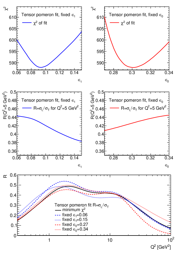
Figure 17: The goodness-of-fit $\chi^{2}$ and the ratio $R=\sigma_{L}/\sigma_{T}$ of longitudinal to transverse cross sections are studied in fits with $24$ free parameters as a function of $\epsilon_{0}$ and $\epsilon_{1}$. The upper panels show $\chi^{2}$ as a function of $\epsilon_{1}$ (left) and $\epsilon_{0}$ (right). The middle panels show $R(Q^{2}=5\,\text{GeV}^{2})$ as a function of $\epsilon_{1}$ (left) and $\epsilon_{0}$ (right). The lower panel shows the $R$ distribution as a function of $Q^{2}$ for extreme choices of the $\epsilon_{j}$. For this study, the energy $W$ is set to $200\,\text{GeV}$.

The scans cover large parameter ranges with a goodness-of-fit up to and above $\chi^{2}=600$, corresponding to parameter variations by more than three standard deviations. The resulting $R$, however, is not affected by so much. Thus, with all necessary caution, we think we can say that the HERA data, fitted with our two-pomeron model, prefer a relatively large value for $R$ in the above $Q^{2}$ range.

References

- [1] C. Adloff et al. [H1 Collaboration], A Measurement of the proton structure function at low x and low at HERA, Nucl. Phys. B 497 (1997) 3 [hep-ex/9703012].
- [2] J. Breitweg et al. [ZEUS Collaboration], Measurement of the proton structure function and at low and very low x at HERA, Phys. Lett. B 407 (1997) 432 [hep-ex/9707025].
- [3] R. Devenish and A. Cooper-Sarkar, Deep inelastic scattering, Oxford University Press (2004).
- [4] A. Donnachie, H. G. Dosch, P. V. Landshoff and O. Nachtmann, Pomeron physics and QCD, Camb. Monogr. Part. Phys. Nucl. Phys. Cosmol. 19 (2002) 1.
- [5] L. Caneschi (ed.), Regge Theory of Low- Hadronic Interactions, Elsevier Science Publishers B. V., Amsterdam 1989.
- [6] M. Haguenauer, B. Nicolescu, and J. Tran Thanh Van (eds.), Proc. XIth International Conference on Elastic and Diffractive Scattering, Towards High Energy Frontiers, Thê Giôi Publishers, Vietnam, 2006.
- [7] V. Barone and E. Predazzi, High-Energy Particle Diffraction, Springer-Verlag, Berlin, Heidelberg, 2002.
- [8] A. Donnachie and P. V. Landshoff, Small x: Two pomerons!, Phys. Lett. B 437 (1998) 408 [hep-ph/9806344].
- [9] A. Donnachie and P. V. Landshoff, New data and the hard Pomeron, Phys. Lett. B 518 (2001) 63 [hep-ph/0105088].
- [10] A. Donnachie and P. V. Landshoff, Does the hard pomeron obey Regge factorisation?, Phys. Lett. B 595 (2004) 393 [hep-ph/0402081].
- [11] C. Ewerz, M. Maniatis and O. Nachtmann, A Model for Soft High-Energy Scattering: Tensor Pomeron and Vector Odderon, Annals Phys. 342 (2014) 31 [arXiv:1309.3478 [hep-ph]].
- [12] H. G. Dosch and E. Ferreira, Scale Dependent Pomeron Intercept in Electromagnetic Diffractive Processes, arXiv:1503.06649 [hep-ph].
- [13] A. Bolz, C. Ewerz, M. Maniatis, O. Nachtmann, M. Sauter and A. Schöning, Photoproduction of pairs in a model with tensor-pomeron and vector-odderon exchange, JHEP 1501 (2015) 151 [arXiv:1409.8483 [hep-ph]].
- [14] P. Lebiedowicz, O. Nachtmann and A. Szczurek, Exclusive central diffractive production of scalar and pseudoscalar mesons; tensorial vs. vectorial pomeron, Annals Phys. 344 (2014) 301 [arXiv:1309.3913 [hep-ph]].
- [15] P. Lebiedowicz, O. Nachtmann and A. Szczurek, and Drell-Söding contributions to central exclusive production of pairs in proton-proton collisions at high energies, Phys. Rev. D 91 (2015) 074023 [arXiv:1412.3677 [hep-ph]].
- [16] P. Lebiedowicz, O. Nachtmann and A. Szczurek, Central exclusive diffractive production of the continuum, scalar and tensor resonances in and scattering within the tensor pomeron approach, Phys. Rev. D 93 (2016) 054015 [arXiv:1601.04537 [hep-ph]].
- [17] P. Lebiedowicz, O. Nachtmann and A. Szczurek, Exclusive diffractive production of via the intermediate and states in proton-proton collisions within tensor pomeron approach, Phys. Rev. D 94 (2016) 034017 [arXiv:1606.05126 [hep-ph]].
- [18] P. Lebiedowicz, O. Nachtmann and A. Szczurek, Central production of in collisions with single proton diffractive dissociation at the LHC, Phys. Rev. D 95 (2017) 034036 [arXiv:1612.06294 [hep-ph]].
- [19] M. Klusek-Gawenda, P. Lebiedowicz, O. Nachtmann and A. Szczurek, From the reaction to the production of pairs in ultraperipheral ultrarelativistic heavy-ion collisions at the LHC, Phys. Rev. D 96 (2017) 094029 [arXiv:1708.09836 [hep-ph]].
- [20] P. Lebiedowicz, O. Nachtmann and A. Szczurek, Towards a complete study of central exclusive production of pairs in proton-proton collisions within the tensor Pomeron approach, Phys. Rev. D 98 (2018) 014001 [arXiv:1804.04706 [hep-ph]].
- [21] C. Ewerz, P. Lebiedowicz, O. Nachtmann and A. Szczurek, Helicity in proton-proton elastic scattering and the spin structure of the pomeron, Phys. Lett. B 763 (2016) 382 [arXiv:1606.08067 [hep-ph]].
- [22] L. Adamczyk et al. [STAR Collaboration], Single Spin Asymmetry in Polarized Proton-Proton Elastic Scattering at 200 GeV, Phys. Lett. B 719 (2013) 62 [arXiv:1206.1928 [nucl-ex]].
- [23] O. Nachtmann, Elementary Particle Physics: Concepts and Phenomena, Springer Verlag, Berlin, 1990.
- [24] L. N. Hand, Experimental Investigation of Pion Electroproduction, Phys. Rev. 129 (1963) 1834.
- [25] L. D. Landau, On the angular momentum of a system of two photons, Dokl. Akad. Nauk Ser. Fiz. 60 (1948) 207.
- [26] C. N. Yang, Selection Rules for the Dematerialization of a Particle Into Two Photons, Phys. Rev. 77 (1950) 242.
- [27] H. Abramowicz et al. [H1 and ZEUS Collaborations], Combination of measurements of inclusive deep inelastic scattering cross sections and QCD analysis of HERA data, Eur. Phys. J. C 75 (2015) no.12, 580 [arXiv:1506.06042 [hep-ex]].
- [28] S. Aid et al. [H1 Collaboration], Measurement of the total photon-proton cross-section and its decomposition at 200 GeV center-of-mass energy, Z. Phys. C 69 (1995) 27 [hep-ex/9509001].
- [29] S. Chekanov et al. [ZEUS Collaboration], Measurement of the photon-proton total cross-section at a center-of-mass energy of 209 GeV at HERA, Nucl. Phys. B 627 (2002) 3 [hep-ex/0202034].
- [30] G. M. Vereshkov, O. D. Lalakulich, Y. F. Novoseltsev and R. V. Novoseltseva, Total cross section for photon-nucleon interaction in the energy range = 40 GeV - 250 GeV, Phys. Atom. Nucl. 66 (2003) 565 [Yad. Fiz. 66 (2003) 591].
- [31] D. O. Caldwell et al., Measurements of the Photon Total Cross-Section on Protons from 18 GeV to 185 GeV, Phys. Rev. Lett. 40 (1978) 1222.
- [32] V. Andreev et al. [H1 Collaboration], Measurement of inclusive cross sections at high at 225 and 252 GeV and of the longitudinal proton structure function at HERA, Eur. Phys. J. C 74 (2014) 2814 [arXiv:1312.4821 [hep-ex]].
- [33] L. V. Gribov, E. M. Levin and M. G. Ryskin, Semihard Processes in QCD, Phys. Rept. 100 (1983) 1.
- [34] M. Froissart, Asymptotic behavior and subtractions in the Mandelstam representation, Phys. Rev. 123 (1961) 1053.
- [35] A. Martin, Extension of the axiomatic analyticity domain of scattering amplitudes by unitarity - I, Nuovo Cim. A 42 (1966) 930.
- [36] L. Lukaszuk and A. Martin, Absolute upper bounds for pi pi scattering, Nuovo Cim. A 52 (1967) 122.
- [37] O. Nachtmann, Effective field theory approach to structure functions at small , Eur. Phys. J. C 26 (2003) 579 [hep-ph/0206284].
- [38] C. Ewerz and O. Nachtmann, Towards a nonperturbative foundation of the dipole picture: II. High energy limit, Annals Phys. 322 (2007) 1670 [hep-ph/0604087].
- [39] C. Ewerz and O. Nachtmann, Bounds on Ratios of DIS Structure Functions from the Color Dipole Picture, Phys. Lett. B 648 (2007) 279 [hep-ph/0611076].
- [40] F. D. Aaron et al. [H1 Collaboration], Measurement of the Inclusive Scattering Cross Section at High Inelasticity y and of the Structure Function , Eur. Phys. J. C 71 (2011) 1579 [arXiv:1012.4355 [hep-ex]].
- [41] C. Ewerz, A. von Manteuffel, O. Nachtmann and A. Schöning, The New Measurement from HERA and the Dipole Model, Phys. Lett. B 720 (2013) 181 [arXiv:1201.6296 [hep-ph]].
- [42] F. J. Yndurain, Quantum Chromodynamics, Springer-Verlag, New York, Heidelberg, 1983.
- [43] V. N. Gribov and L. N. Lipatov, Deep inelastic scattering in perturbation theory, Sov. J. Nucl. Phys. 15 (1972) 438 [Yad. Fiz. 15 (1972) 781].
- [44] G. Altarelli and G. Parisi, Asymptotic Freedom in Parton Language, Nucl. Phys. B 126 (1977) 298.
- [45] Y. L. Dokshitzer, Calculation of the Structure Functions for Deep Inelastic Scattering and Annihilation by Perturbation Theory in Quantum Chromodynamics, Sov. Phys. JETP 46 (1977) 641 [Zh. Eksp. Teor. Fiz. 73 (1977) 1216].
- [46] A. Donnachie and P. V. Landshoff, Perturbative QCD and Regge theory: Closing the circle, Phys. Lett. B 533 (2002) 277 [hep-ph/0111427].
- [47] E. A. Kuraev, L. N. Lipatov and V. S. Fadin, The Pomeranchuk Singularity in Nonabelian Gauge Theories, Sov. Phys. JETP 45 (1977) 199 [Zh. Eksp. Teor. Fiz. 72 (1977) 377].
- [48] I. I. Balitsky and L. N. Lipatov, The Pomeranchuk Singularity in Quantum Chromodynamics, Sov. J. Nucl. Phys. 28 (1978) 822 [Yad. Fiz. 28 (1978) 1597].
- [49] I. Abt, A. M. Cooper-Sarkar, B. Foster, V. Myronenko, K. Wichmann and M. Wing, Study of HERA ep data at low Q2 and low and the need for higher-twist corrections to standard perturbative QCD fits, Phys. Rev. D 94 (2016) 034032 [arXiv:1604.02299 [hep-ph]].
- [50] A. Luszczak and H. Kowalski, Dipole model analysis of highest precision HERA data, including very low ’s Phys. Rev. D 95 (2017) 014030 [arXiv:1611.10100 [hep-ph]].
- [51] R. D. Ball, V. Bertone, M. Bonvini, S. Marzani, J. Rojo and L. Rottoli, Parton distributions with small-x resummation: evidence for BFKL dynamics in HERA data, Eur. Phys. J. C 78 (2018) 321 [arXiv:1710.05935 [hep-ph]].
- [52] H. Abdolmaleki et al. [xFitter Developers’ Team], Impact of low- resummation on QCD analysis of HERA data, Eur. Phys. J. C 78 (2018) 621 [arXiv:1802.00064 [hep-ph]].
- [53] C. Ewerz and O. Nachtmann, Towards a nonperturbative foundation of the dipole picture: I. Functional methods, Annals Phys. 322 (2007) 1635 [hep-ph/0404254].
- [54] C. Ewerz, A. von Manteuffel and O. Nachtmann, On the Energy Dependence of the Dipole-Proton Cross Section in Deep Inelastic Scattering, JHEP 1103 (2011) 062 [arXiv:1101.0288 [hep-ph]].
- [55] A. Accardi et al., Electron Ion Collider: The Next QCD Frontier : Understanding the glue that binds us all, Eur. Phys. J. A 52 (2016) 268 [arXiv:1212.1701 [nucl-ex]].
- [56] J. L. Abelleira Fernandez et al. [LHeC Study Group], A Large Hadron Electron Collider at CERN: Report on the Physics and Design Concepts for Machine and Detector, J. Phys. G 39 (2012) 075001 [arXiv:1206.2913 [physics.acc-ph]].
- [57] D. Britzger et al., The ALPOS fit framework, available at http://www.desy.de/~britzger/alpos/.
- [58] F. James and M. Roos, Minuit: A System for Function Minimization and Analysis of the Parameter Errors and Correlations, Comput. Phys. Commun. 10 (1975) 343.
- [59] B. List for the H1 Collaboration, Extraction of the Pomeron Trajectory from a Global Fit to Exclusive Meson Photoproduction Data, in Proceedings of the XVII International Workshop on Deep Inelastic Scattering and Related Subjects DIS 2009, Madrid, Spain, April 26-30, 2009, arXiv:0906.4945 [hep-ex].
- [60] S. Alekhin et al., HERAFitter, Eur. Phys. J. C 75 (2015) 304 [arXiv:1410.4412 [hep-ph]].
- [61] https://www.xfitter.org/xFitter/
- [62] J. Pumplin, D. R. Stump and W. K. Tung, Multivariate fitting and the error matrix in global analysis of data, Phys. Rev. D 65 (2001) 014011 [hep-ph/0008191].