Even simpler modeling of quadruply lensed quasars (and random quartets) using Witt’s hyperbola

Abstract

Witt (1996) has shown that for an elliptical potential, the four images of a quadruply lensed quasar lie on a rectangular hyperbola that passes through the unlensed quasar position and the center of the potential as well. Wynne and Schechter (2018) have shown that, for the singular isothermal elliptical potential (SIEP), the four images also lie on an “amplitude” ellipse centered on the quasar position with axes parallel to the hyperbola’s asymptotes. Witt’s hyperbola arises from equating the directions of both sides of the lens equation. The amplitude ellipse derives from equating the magnitudes. One can model any four points as an SIEP in three steps. 1. Find the rectangular hyperbola that passes through the points. 2. Find the aligned ellipse that also passes through them. 3. Find the hyperbola with asymptotes parallel to those of the first that passes through the center of the ellipse and the pair of images closest to each other. The second hyperbola and the ellipse give an SIEP that predicts the positions of the two remaining images where the curves intersect. Pinning the model to the closest pair guarantees a four image model. Such models permit rapid discrimination between gravitationally lensed quasars and random quartets of stars.

1 Introduction

Wynne and Schechter (2018; henceforth WS) describe a robust scheme for generating a singular isothermal elliptical potential (henceforth SIEP) from the image positions of a quadruply lensed quasar. It converges even when the fit is poor or the model parameters improbable. It may be useful both in searching catalogs for gravitationally lensed quasars (e.g. Delchambre et al 2019; Williams et al 2017, 2018; Agnello et al 2018; and Lemon et al 2018) and in providing a first guess for more sophisticated models (e.g. Keeton 2001).

Their method predicts images at the points of intersection of Witt’s (1996) hyperbola, and an “amplitude” ellipse. The asymptotes of the hyperbola, and the axes of both the potential and the amplitude ellipse are all parallel to each other. We call any frame with axes parallel to these an “aligned” frame (as distinct from the “observed” frame of the sky).

The WS scheme finds the amplitude ellipse iteratively, and has the shortcoming that quartets of points sometimes result in SIEP models that produce only two images. We present here a simpler variant of the WS approach that constructs an SIEP model without iteration and which ensures four images. It permits yet more rapid discrimination between lensed quasars and random quartets of stars.

2 The SIEP, the amplitude ellipse and Witt’s hyperbola

The two-dimensional effective potential $\psi$ (e.g. Schneider et al 1992) for an SIEP centered on a lensing galaxy at $(x_{g},y_{g})$, is given by

$$\psi=a^{2}\left[{(x-x_{g})^{2}\over a^{2}}+{(y-y_{g})^{2}\over q^{2}a^{2}}\right]^{1/2}\quad,$$ (1)

in an aligned frame, where $q$ is the ratio of the $y$ semiaxis to the $x$ semiaxis. The $x$ semiaxis, $a$, is either the the semi-major axis of the potential if $q<1$ or its semi-minor axis if $q>1$.

The amplitude ellipse is centered on the source at $(x_{s},y_{s})$ and is given by

$${(x-x_{s})^{2}\over a^{2}}+{(y-y_{s})^{2}\over a^{2}/q^{2}}=1$$ (2)

in an aligned frame, where $1/q$ is the ratio of its y-semiaxis to its x-semiaxis. It is orthogonal to the elliptical potential and has the same shape, but has a larger semi-major axis.

The hyperbola is offset from both the potential and the amplitude ellipse. For an elliptical potential in an aligned frame it is given by Witt’s equation,

$$(x-x_{g})(y-y_{s})={1\over q^{2}}(y-y_{g})(x-x_{s})\quad,$$ (3)

from which one sees that both the lensing galaxy and the source lie on the hyperbola. The coordinates of the center of the hyperbola, $(x_{h},y_{h})$, are found to be

$$x_{h}={(-y_{s}+q^{2}y_{g})\over(1-q^{2})}\quad;\quad y_{h}={(-x_{s}+q^{2}x_{g})\over(1-q^{2})}$$ (4)

in an aligned frame. The semi-major axis of the hyperbola, is equal to $\sqrt{|c^{2}|}$, where

$$c^{2}\equiv-2{q^{2}\over 1-q^{2}}(x_{s}-x_{g})(y_{s}-y_{g})\quad.$$ (5)

The hyperbola’s semi-major axis is parallel to the line $y=x$ if $c^{2}>0$ and is otherwise parallel to the line $y=-x$. The hyperbola collapses to two perpendicular lines when the displacement of the source from the center of the potential is parallel to either of the axes of an aligned frame. Witt’s equation holds for all elliptical potentials.

In what follows we describe a variant of the WS scheme that is even simpler by virtue of solving directly for the amplitude ellipse rather than iteratively. It also reproduces, by construction, the separation of the closest pair of images, upon which their predicted fluxes strongly depend.

3 The method

We first present our recipe, then elaborate on it and finally explain it.

3.1 The recipe

1. Find the rectangular hyperbola passing through the four image positions in the observed frame;

2. find the image coordinates in an “aligned” frame with axes parallel to the asymptotes of the hyperbola;

3. find the amplitude ellipse passing through the four image positions and aligned with these axes;

4. find the two images subtending the smallest angle from the center of the amplitude ellipse;

5. evaluate Witt’s equation at the positions of these two images to solve for the unknown coordinates of the lensing galaxy, $(x_{g},y_{g})$.

Figure 1: HST F814W images of SDSSJ1330+1810 and PSJ0630-1210. The ellipses and hyperbolae for the models are shown, with images predicted where they intersect. A black circle marks the source position and an “x” marks the galaxy position. By construction the model exactly reproduces the closest image pair. The semi-major axes of the ellipses are $0\farcs 97$ and $1\farcs 44$ respectively. The observed position of the galaxy in SDSSJ1330+1810 lies close to the inferred position, and its orientation is likewise close to the model’s. PSJ0630-1210 has two lensing galaxies, one very close to the inferred source position and one just inside the ellipse near the northernmost image. A fifth quasar image lies between the two galaxies. The hyperbola has so small a semi-major axis, $0\farcs 04$, that it merges with its asymptotes.

3.2 Elaboration

Note that Witt’s equation again describes a hyperbola, with the source and the galaxy on its “primary” branch. By construction the two closest images lie on the secondary branch. The other two images are offset from the primary branch. We take the rms offset of the four images from their predicted positions (normalized by the semi-major axis of the amplitude ellipse), as a figure of merit, $G$, for the SIEP model.

The WS SIEP model differs from the present one in that their hyperbola passes through all four images, and their iteratively fit ellipse passes through none (except when the fit is perfect). In the present, non-iterative scheme, it is the ellipse that passes through all four images, with our final hyperbola passing through only two. It is faster by virtue of its non-iterative nature. Moreover, it reproduces, by construction, the separation of the closest pair of images, which has a strong influence on their predicted fluxes.

The rectangular hyperbola and the amplitude ellipse are found using their representations as conic sections, $Ax^{2}+Bxy+Cy^{2}+Dx+Ey+F=0$, in the observed and aligned frames, respectively. The rectangular hyperbola of the first step has coefficients $A_{h}$ and $C_{h}$ equal and opposite. The coefficient $B_{h}$ may be set equal to unity. Evaluating the conic at the four image positions gives equations that are linear in the four remaining unknowns, $A_{h}$, $D_{h}$, $E_{h}$ and $F_{h}$. In the present scheme only $A_{h}$ is used, giving the angle that an aligned frame makes with the observed frame,

$$\theta=-{1\over 2}\arctan{2A_{h}}$$ (6)

The amplitude ellipse will have $A_{e}=1$ and $B_{e}=0$ in an aligned frame, again giving four equations linear in four unknowns, $C_{e}$, $D_{e}$, $E_{e}$, and $F_{e}$ when evaluated at the four image positions. If $C_{e}<0$, the resulting conic section is a hyperbola, not an ellipse, and is unlikely to have resulted from an SIEP-like potential. This was the case for roughly one third of the random configurations considered below. We extract the square of the axis ratio of the potential, $q^{2}=C_{e}$.

Following Witt’s example, one can further simplify the calculation by taking the origin of the “observed” frame to be one of the four images, in which case the coefficient $F_{h}=0$. One finds the hyperbola by evaluating the conic at the other three images. This trick likewise simplifies solving for the amplitude ellipse if one rotates about Witt’s origin to transform from the observed frame to the the aligned frame. The coefficient $F_{e}$ is then zero and one solves for the amplitude ellipse by evaluating the conic at the other three images.

3.3 Explanation

Both the hyperbola and the amplitude ellipse derive from the “lens equation” (Schneider et al 1992), which sets the image deflection equal to the gradient of a two-dimensional gravitational potential. Witt’s hyperbola is obtained by equating the directions of the two sides of the lens equation. The amplitude ellipse is obtained by equating the magnitudes of the two sides. A proper solution of the lens equation must satisfy both components. Any elliptical potential will have its images, source and galaxy on a rectangular hyperbola (Witt 1996), but only for the SIEP do the images also lie on an associated ellipse with the source at the center.

Figure 2: The red line shows the distribution of the figure of merit $G$ for the 29 known lenses in WS. The black line shows the same distribution for 70 random quartets. The remaining 30 could not be modeled as an SIEP.

4 Application

Figure 3: Three random quartets of points. The first quartet is fit unusually well by the SIEP model. The second quartet is typical of those for which our procedure yielded an SIEP model. The third is typical of those for which the conic section of our third step gave a hyperbola (thin lines) rather than the anticipated amplitude ellipse. The rectangular hyperbola from our first step (thicker lines) has three images on one branch and one on the other, rather than two on each.

4.1 Known quadruply lensed quasars

We have applied the above technique to the 29 systems analyzed in WS. These yielded SIEP models very similar to those in WS for the better fitting systems but agreed less well for those with poorer fits.

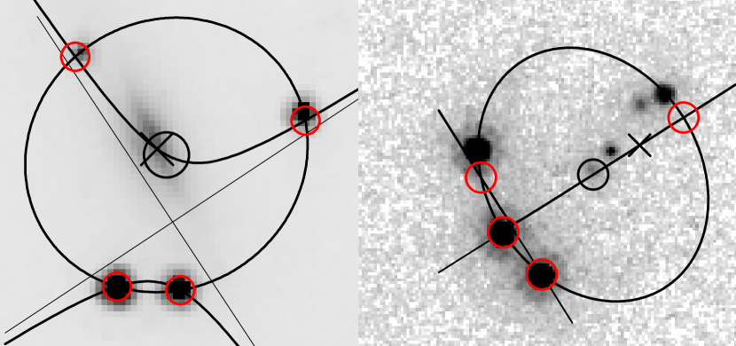
In Figure 1 we show the result of applying the present technique to the gravitationally lensed quasars SDSSJ1330+1801 (Oguri et al 2008) and PSJ0630-1201 (Ostrovski et al 2017), with positions taken from Shajib et al (2019). These gave two of the three worst WS fits, with their amplitude ellipses intersecting only the primary branch of the hyperbola, producing just two images. Random quartets exhibit this pathology more frequently. Source plane fitting algorithms, which minimize the scatter in the positions inferred for the source for each of the four images, can also predict two rather than four images.

This renders the WS approach ill-suited to using observed fluxes to further discriminate between quadruply lensed quasars and random quartets. By construction the present method produces four images, with the distance between the two closest images exactly as observed. Close pairs indicate a source that lies near a fold caustic (Gaudi and Petters 2002), with the magnification of the pair varying inversely as the distance between them.

4.2 Random quartets

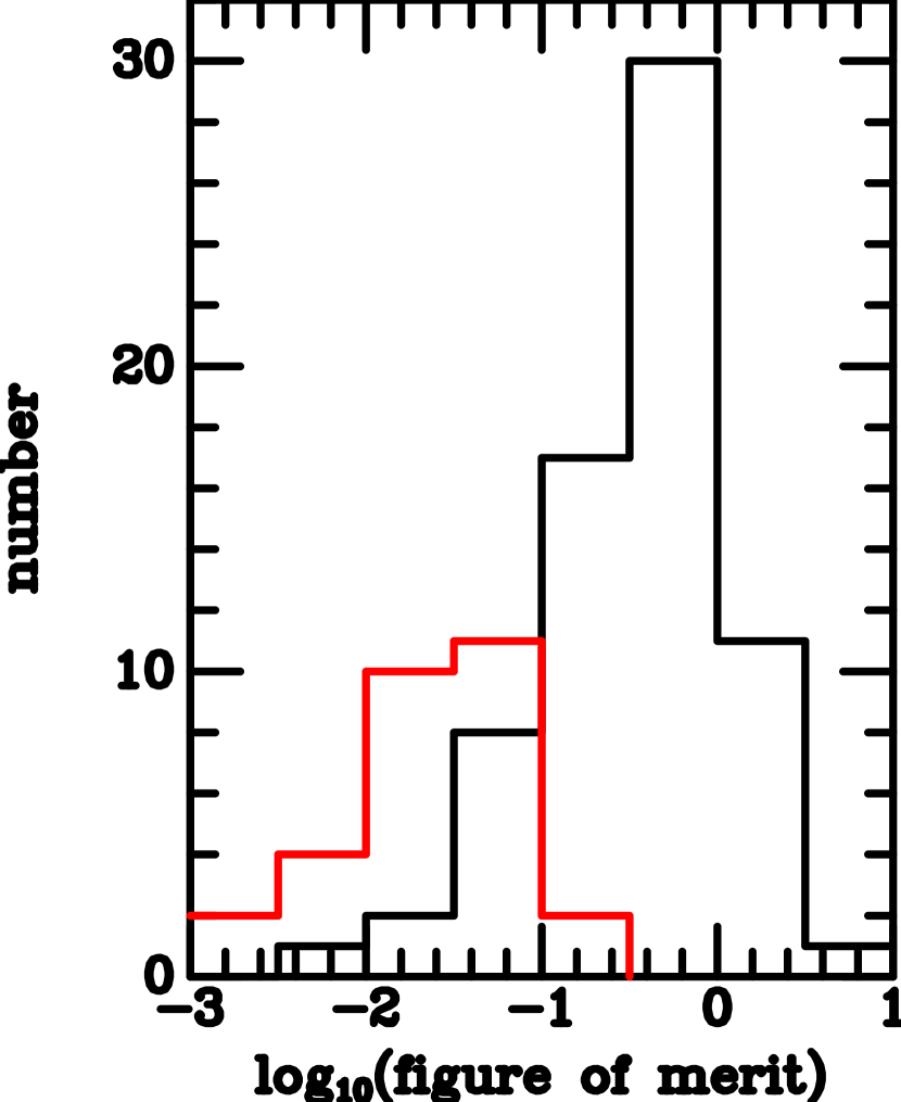
We attempted to produce SIEP models for the same 100 random quartets analyzed in WS. As noted above, no amplitude ellipse could be drawn through roughly 1/3 of these, with the third step yielding a hyperbola instead. In Figure 2 we show a histogram of the figure of merit $G$ for the surviving random quartets and for the 29 known lenses. While the present figure of merit is roughly a factor of two smaller than that of WS, for both the known lenses and the random quartets, they produce similar rank orderings. If we reject systems with $G>0.1$ we lose two known lenses (both of which have two lensing galaxies) and accept eleven random quartets. If we further reject systems with axis ratios outside the interval $0.4<q<2.5$, the false positive rate drops to 8% without losing any more known lenses, the most extreme of which, 2M1134-2103, has $q=0.49$.

Lucey et al (2017) attribute the quadrupole moment in 2M1134-2103 to an external shear, $\gamma=0.34$, rather than to an elliptical mass distribution, which would have an axis ratio $q_{m}\sim 0.1$. Using Keeton’s (2001) lensmodel program we have generated many synthetic quartets assuming a singular isothermal sphere with external shear. We consistently find $q=(1-\gamma)/(1+\gamma)$, with the SIEP giving perfect fits to these synthetic quartets. Our cutoff of $q=0.4$ corresponds to a shear $\gamma=0.429$, larger than any known for a lensed quasar.

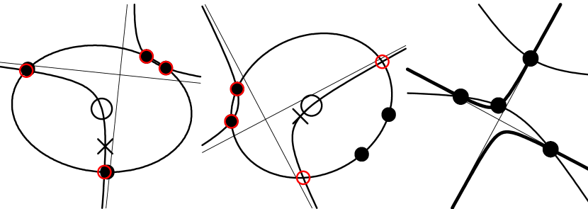
In Figure 3 we show models for three random quartets of points. The first quartet has $G=0.028$, better than most of the known lenses. The second has $G=0.598$, typical of the random quartets and substantially worse than the known lenses. The third quartet was among those for which no SIEP model could be found. For this system we show the hyperbola derived from the first step and the unwanted hyperbola derived from the attempt to find an amplitude ellipse.

For an SIEP, the amplitude ellipse is centered on the primary branch of Witt’s hyperbola, and must intersect it in at least two points. It may or may not intersect the secondary branch, but will do so twice when it does. Yet for the third quartet, three of the four random points lie on one branch of Witt’s hyperbola. It is no surprise that an SIEP model could not be found

5 Using fluxes to improve discrimination between quadruply lensed quasars and random quartets

Delchambre et al (2019) catalog 70,000 quartets of GAIA point sources, from which they recover eleven known quadruply lensed quasars and find at least one new confirmed quad. Their “extremely randomized trees” method (ERT) does better at finding these than the present approach, with the twelve confirmed lenses ranked higher than 1440 and 5600 in their ranked list of quads and ours, respectively. This may be explained by the implicit use of both flux ratios and positions by the ERT algorithm, where the present method uses only positions.

While the second and third random quartets in Figure 3 are not likely to be mistaken for a lensed quasar, the first quartet is an excellent impostor if one considers only positions. But if one uses the SIEP model to predict fluxes, one finds that the two close images are highly magnified and very nearly equal in magnitude. The next brightest is 1.5 magnitudes fainter, and the least bright, close to the lensing galaxy, is 4 magnitudes fainter. While the flux ratios for a random quartet of stars will depend upon its Galactic coordinates and the depth of the survey, they are unlikely to match this pattern.

Unfortunately, fluxes for the individual macro-images predicted by an SIEP model are subject to micro-lensing by the stars in the lensing galaxy (Paczyński 1986). Therefore SIEP-predicted fluxes may not improve discrimination as much as might otherwise be thought. Macro-images may deviate by two magnitudes or more depending upon the convergences and shears at their positions (which are known from the SIEP model) and the surface mass density of micro-lenses (Wambsganss 1992), which even under the simplest of assumptions depends upon the redshifts of the source and lens. Taking these effects into account is more computationally intensive than the present discrimination based only on positions.

A further complication in using fluxes is our inability to distinguish between an SIEP configuration and an externally sheared singular isothermal sphere when considering only positions. The two alternatives give flux ratios that can vary by 20-30%. Moreover, the absolute magnifications are to first order a factor of two greater in the case of external shear, so the effects of micro-lensing will be different in the two cases.

These complications notwithstanding, flux ratios are likely to provide at least some improvement in discriminating between quadruply lensed quasars and random quartets.

References

- Agnello et al. (2018) Agnello, A., Lin, H., Kuropatkin, N., et al. 2018, MNRAS, 479, 4345
- Delchambre et al. (2019) Delchambre, L., Krone-Martins, A., Wertz, O., et al. 2019, A&A, 622, A165
- Deutsch (1966) Deutsch, A. J. 1966, Abundance Determinations in Stellar Spectra, 26, 112
- Gaudi & Petters (2002) Gaudi, B. S., & Petters, A. O. 2002, ApJ, 574, 970
- Keeton (2001) Keeton, C. R. 2001, arXiv:astro-ph/0102340
- Lemon et al. (2018) Lemon, C. A., Auger, M. W., McMahon, R. G., & Ostrovski, F. 2018, MNRAS, 479, 5060
- Lucey et al. (2018) Lucey, J. R., Schechter, P. L., Smith, R. J., & Anguita, T. 2018, MNRAS, 476, 927
- Oguri et al. (2008) Oguri, M., Inada, N., Blackburne, J. A., et al. 2008, MNRAS, 391, 1973
- Ostrovski et al. (2018) Ostrovski, F., Lemon, C. A., Auger, M. W., et al. 2018, MNRAS, 473, L116
- Paczynski (1986) Paczyński, B. 1986a, ApJ, 301, 503
- Schneider et al. (1992) Schneider, P., Ehlers, J., & Falco, E. E. 1992, Gravitational Lenses, XIV, 560 pp. 112 figs.. Springer-Verlag Berlin Heidelberg New York. Also Astronomy and Astrophysics Library, 112
- Shajib et al. (2019) Shajib, A. J., Birrer, S., Treu, T., et al. 2019, MNRAS, 483, 5649.
- Wambsganss (1992) Wambsganss, J. 1992, ApJ, 386, 19
- Williams et al. (2017) Williams, P., Agnello, A., & Treu, T. 2017, MNRAS, 466, 3088
- Williams et al. (2018) Williams, P. R., Agnello, A., Treu, T., et al. 2018, MNRAS, 477, L70
- Witt (1996) Witt, H. J. 1996, ApJ, 472, L1
- Wynne & Schechter (2018) Wynne, R. A., & Schechter, P. L. 2018, arXiv:1808.06151