Abstract

We present a novel algorithm for overcomplete independent components analysis (ICA), where the number of latent sources $k$ exceeds the dimension $p$ of observed variables. Previous algorithms either suffer from high computational complexity or make strong assumptions about the form of the mixing matrix. Our algorithm does not make any sparsity assumption yet enjoys favorable computational and theoretical properties. Our algorithm consists of two main steps: (a) estimation of the Hessians of the cumulant generating function (as opposed to the fourth and higher order cumulants used by most algorithms) and (b) a novel semi-definite programming (SDP) relaxation for recovering a mixing component. We show that this relaxation can be efficiently solved with a projected accelerated gradient descent method, which makes the whole algorithm computationally practical. Moreover, we conjecture that the proposed program recovers a mixing component at the rate $k<p^{2}/4$ and prove that a mixing component can be recovered with high probability when $k<(2-\varepsilon)p\log p$ when the original components are sampled uniformly at random on the hypersphere. Experiments are provided on synthetic data and the CIFAR-10 dataset of real images.

1 Introduction

Independent component analysis (ICA) models a $p$-dimensional observation $x$ as a linear combination of $k$ latent mutually independent sources:

$$x=D\alpha,$$ (1)

where $\alpha:=(\alpha_{1},\dots,\alpha_{k})^{\top}$ and $D\in\mathbb{R}^{p\times k}$. The linear transformation $D$ is called the mixing matrix and is closely related to the dictionary matrix from dictionary learning (see, e.g., Chen and Donoho, 1994; Chen et al., 1998). Given a sample $X:=\{x^{(1)},\dots,x^{(n)}\}$ of $n$ observations, one is often interested in estimating the latent mixing matrix $D$ and respective latent representations, $\alpha^{(1)},\dots,\alpha^{(n)}$, also known as sources, of every observation.

A classical motivating example for ICA is the cocktail party problem, where one is interested in separating individual speakers’ voices from noisy recordings. Here, each record is an observation and each speaker is an independent source. In general, ICA is a simple single-layered neural network and is widely used as an unsupervised learning method in machine learning and signal processing communities (see, e.g., Hyvärinen et al., 2001; Comon and Jutten, 2010).

There are three conceptually different settings of the ICA problem: (a) complete, or determined, where the dimension of observations coincides with the number of sources, i.e., $p=k$; (b) undercomplete, or overdetermined, with fewer sources than the dimension, i.e., $k<p$; and (c) overcomplete, or underdetermined, with more sources than the dimension, i.e., $k>p$. While the first two cases are well studied, the last one is more difficult and we address it here.

In the complete setting, where $k=p$, ICA is usually solved via pre-whitening of the data so that the whitened observations, $z:=Wx$, are uncorrelated and all have unit variance, i.e., $\mathrm{cov}(z)=W\mathrm{cov}(x)W^{\top}=I$, where $W$ denotes the whitening matrix. Substituting $x=D\alpha$, we get $(WD)(WD)^{\top}=I$ which implies that the matrix $Q:=WD$ is orthogonal and therefore the problem of finding the mixing matrix $D$ boils down to finding the “correct” orthogonal matrix $Q$. Numerous “correctness” criteria, such as maximizing non-Gaussianity of sources, were proposed and respective algorithms for complete ICA are well known (see, e.g., Hyvärinen et al., 2001; Comon and Jutten, 2010). The most widely known complete ICA algorithms are possibly the FastICA algorithm by Hyvärinen (1999) and the JADE algorithm by Cardoso and Souloumiac (1993). This naturally extends to the undercomplete setting where one looks for an orthonormal matrix, where columns are orthogonal, instead. However, although nothing prevents us from whitening data in the overcomplete setting, the orthogonalization trick cannot be extended to the overcomplete setting, where $k>p$, since the mixing matrix $D$ has more columns than rows and therefore cannot have full column rank.

Improvements in feature learning are among the advantages of overcomplete representations: it has been shown by Coates et al. (2011) that dense and overcomplete features can significantly improve performance of classification algorithms. However, advantages of overcomplete representations go far beyond this task (see, e.g., Bengio et al., 2013).

Originally, the idea of overcomplete representations was developed in the context of dictionary learning, where an overcomplete dictionary, formed by Fourier, wavelet, Gabor or other filters, is given and one is only interested in estimating the latent representations $\alpha$. Different approaches were proposed for this problem including the method of frames (Daubechies, 1988) and basis pursuit (Chen and Donoho, 1994; Chen et al., 1998). Later in sparse coding, the idea of estimating a dictionary matrix directly from data was introduced (Olshausen and Field, 1996, 1997) and was shortly followed by the first overcomplete ICA algorithm (Lewicki and Sejnowski, 2000). Further overcomplete ICA research continued in several fairly different directions based on either (a) various sparsity assumptions (see, e.g., Teh et al., 2003) or on (b) prior assumptions about the sources as by Lewicki and Sejnowski (2000) or (c) instead in a more general dense overcomplete setting (see, e.g., Hyvärinen, 2005; Comon and Rajih, 2006; De Lathauwer et al., 2007; Goyal et al., 2014; Bhaskara et al., 2014a, b; Anandkumar et al., 2015; Ma et al., 2016). Since we focus on this more general dense setting, we do not review or compare to the literature in the other settings.

In particular, we focus on the following problem: Estimate the mixing matrix $D$ given an observed sample $X:=\left\{x^{(1)},\dots,x^{(n)}\right\}$ of $n$ observations. We aim at constructing an algorithm that would bridge the gap between algorithms with theoretical guarantees and ones with practical computational properties. Notably, our algorithm does not depend on any probabilistic assumptions on the sources, except for the standard independence and non-Gaussianity, and the uniqueness of the ICA representation (up to permutation and scaling) is the result of the independence of sources rather than sparsity. Here we only focus on the estimation of the latent mixing matrix and leave the learning of the latent representation for future research (note that one can use, e.g., the mentioned earlier dictionary learning approaches).

Different approaches have been proposed to address this problem. Some attempt to relax the hard orthogonality constraint in the whitening procedure with more heuristic quasi-orthogonalization approaches (see, e.g., Le et al., 2011; Arora et al., 2012). Other approaches try to specifically address the structure of the model in the overcomplete setting (see, e.g., Hyvärinen, 2005; Comon and Rajih, 2006; De Lathauwer et al., 2007; Goyal et al., 2014; Bhaskara et al., 2014a, b; Anandkumar et al., 2015; Ma et al., 2016) by considering higher-order cumulants or derivatives of the cumulant generating function. The algorithm that we propose is the closest to the latter type of approach.

Algorithm 1 OverICA

1:Input: Observations $X:=\left\{x_{1},\dots,x_{n}\right\}$ and latent dimension $k$.

2:Parameters: The regularization parameter $\mu$ and the number $s$ of generalized covariances, $s>k$.

3:STEP I. Estimation of the subspace $W$:

4:Sample vectors $t_{1},\dots,t_{s}$.

5:Estimate matrices $H_{j}:=\mathcal{C}_{x}(t_{j})$ for all $j\in[s]$.

6:STEP II. Estimation of the atoms:

7:Given $G^{(i)}$ for every deflation step $i=1,2,\dots,k$:

8:Solve the relaxation (12) with $G^{(i)}$.

9:(OR: Solve the program (9) with $G^{(i)}$.)

10:Estimate the $i$-th mixing component $d_{i}$ from $B^{\ast}$.

11:Output: Mixing matrix $D=(d_{1},d_{2},\dots,d_{k})$.

We make two conceptual contributions: (a) we show how to use second-order statistics instead of the fourth and higher-order cumulants, which improves sample complexity, and (b) we introduce a novel semi-definite programming-based approach, with a convex relaxation that can be solved efficiently, for estimating the columns of $D$. Overall, this leads to a computationally efficient overcomplete ICA algorithm that also has theoretical guarantees. Conceptually, our work is similar to the fourth-order only blind identification (FOOBI) algorithm (De Lathauwer et al., 2007), which we found to work well in practice. However, FOOBI suffers from high computational and memory complexities, its theoretical guarantee requires all kurtoses of the sources to be positive, and it makes the strong assumption that certain fourth-order tensors are linearly independent. Our approach resolves these drawbacks. We describe our algorithm in Section 2 and experimental results in Section 3.

2 Overcomplete ICA via SDP

2.1 Algorithm overview

We focus on estimating the latent mixing matrix $D\in\mathbb{R}^{p\times k}$ of the ICA model (1) in the overcomplete setting where $k>p$. We first motivate our algorithm in the population (infinite sample) setting and later address the finite sample case.

In the following, the $i$-th column of the mixing matrix $D$ is denoted as $d_{i}$ and called the $i$-th mixing component. The rank-1 matrices $d_{1}d_{1}^{\top},\dots,d_{k}d_{k}^{\top}$ are referred to as atoms.

Our algorithm, referred to as OverICA, consists of two major steps: (a) construction of the subspace $\mathbf{W}$ spanned by the atoms, i.e.,

$$W:=\mathrm{Span}\left\{d_{1}d_{1}^{\top},\dots,d_{k}d_{k}^{\top}\right\},\vspace{-2mm}$$ (2)

and $(b)$ estimation of individual atoms $d_{i}d_{i}^{\top}$, $i\in[k]$, given any basis of this subspace. We summarize this high level idea in Algorithm 1. Note that although the definition of the subspace $W$ in (2) is based on the latent atoms, in practice this subspace is estimated from the known observations $x$ (see Section 2.3). However, we do use this explicit representation in our theoretical analysis.

In general, there are different ways to implement these two steps. For instance, some algorithms implement the first step based on the fourth or higher order cumulants (see, e.g., De Lathauwer et al., 2007; Goyal et al., 2014). In contrast, we estimate the subspace $W$ from the Hessian of the cumulant generating function which has better computational and sample complexities (see Section 2.3). Our algorithm also works (without any adjustment) with other implementations of the first step, including the fourth-order cumulant based one, but other algorithms cannot take advantage of our efficient first step due to the differences in the second step.

In the second step, we propose a novel semi-definite program (SDP) for estimation of an individual atom given the subspace $W$ (Section 2.4.1). We also provide a convex relaxation of this program which admits efficient implementation and introduces regularization to noise which is handy in practice when the subspace $W$ can only be estimated approximately (Section 2.4.2). Finally, we provide a deflation procedure that allows us to estimate all the atoms (Section 2.4.3). Before proceeding, a few assumptions are in order.

2.2 Assumptions

Due to the inherent permutation and scaling unidentifiability of the ICA problem, it is a standard practice to assume, without loss of generality, that

Assumption 2.1.

Every mixing component has unit norm, i.e., $\left\|d_{i}\right\|_{2}=1$ for all $i\in[k]$.

This assumption immediately implies that all atoms have unit Frobenius norm, i.e., $\left\|d_{i}d_{i}^{\top}\right\|_{F}=\left\|d_{i}\right\|_{2}^{2}=1$ for all $i\in[k]$.

Since instead of recovering mixing components $d_{i}$ as in (under-) complete setting we recover atoms $d_{i}d_{i}^{\top}$, the following assumption is necessary for the identifiability of our algorithm:

Assumption 2.2.

The matrices (atoms) $d_{1}d_{1}^{\top}$, $d_{2}d_{2}^{\top}$, …, $d_{k}d_{k}^{\top}$ are linearly independent.

This in particular implies that the number of sources $k$ cannot exceed $m:=p(p+1)/2$, which is the latent dimension of the set of all symmetric matrices $\mathcal{S}_{p}$. We also assume, without loss of generality, that the observations are centred, i.e., $\mathbb{E}(x)=\mathbb{E}(\alpha)=0$.

2.3 Step I: Subspace Estimation

In this section, we describe a construction of an orthonormal basis of the subspace $W$. For that, we first construct matrices $H_{1},\dots,H_{s}\in\mathbb{R}^{p\times p}$, for some $s$, which span the subspace $W$. These matrices are obtained from the Hessian of the cumulant generating function as described below.

Generalized Covariance Matrices.

Introduced for complete ICA by Yeredor (2000), a generalized covariance matrix is the Hessian of the cumulant generating function evaluated at a non-zero vector.

Recall that the cumulant generating function (cfg) of a $p$-valued random variable $x$ is defined as

$$\phi_{x}(t):=\log\mathbb{E}(e^{t^{\top}x}),\vspace{-2.3mm}$$ (3)

for any $t\in\mathbb{R}^{p}$. It is well known that the cumulants of $x$ can be computed as the coefficients of the Taylor series expansion of the cgf evaluated at zero (see, e.g., Comon and Jutten, 2010, Chapter 5). In particular, the second order cumulant, which coincides with the covariance matrix, is then the Hessian evaluated at zero, i.e., $\mathrm{cov}(x)=\nabla^{2}\phi_{x}(0)$.

The generalized covariance matrix is a straightforward extension where the Hessian of the cgf is evaluated at a non-zero vector $t$:

$$\mathcal{C}_{x}(t):=\nabla^{2}\phi_{x}(t)=\frac{\mathbb{E}(xx^{\top}e^{t^{\top}x})}{\mathbb{E}(e^{t^{\top}x})}-\mathcal{E}_{x}(t)\mathcal{E}_{x}(t)^{\top},\vspace{-3mm}$$ (4)

where we introduced

$$\mathcal{E}_{x}(t):=\nabla\phi_{x}(t)=\frac{\mathbb{E}(xe^{t^{\top}x})}{\mathbb{E}(e^{t^{\top}x})}.$$ (5)

Generalized Covariance Matrices of ICA.

In case of the ICA model, substituting (1) into the expressions (5) and (4), we obtain

$$\mathcal{E}_{x}(t) =\frac{D\mathbb{E}(\alpha e^{\alpha^{\top}y})}{\mathbb{E}(e^{\alpha^{\top}y})}=D\mathcal{E}_{\alpha}(y),$$ (6)

$$\mathcal{C}_{x}(t) =D\mathcal{C}_{\alpha}(y)D^{\top},$$

where we introduced $y:=D^{\top}t$ and the generalized covariance $\mathcal{C}_{\alpha}(y):=\nabla^{2}\phi_{\alpha}(y)$ of the sources:

$$\mathcal{C}_{\alpha}(y)=\frac{\mathbb{E}(\alpha\alpha^{\top}e^{\alpha^{\top}y})}{\mathbb{E}(e^{\alpha^{\top}y})}-\mathcal{E}_{\alpha}(y)\mathcal{E}_{\alpha}(y)^{\top},\vspace{-1mm}$$ (7)

where $\mathcal{E}_{\alpha}(y):=\nabla\phi_{\alpha}(y)=\mathbb{E}(\alpha e^{y^{\top}\alpha})/\mathbb{E}(e^{y^{\top}\alpha})$.

Importantly, the generalized covariance $\mathcal{C}_{\alpha}(y)$ of the sources, due to the independence, is a diagonal matrix (see, e.g., Podosinnikova et al., 2016). Therefore, the ICA generalized covariance $\mathcal{C}_{x}(t)$ is:

$$C_{x}(t)=\sum_{i=1}^{k}\omega_{i}(t)d_{i}d_{i}^{\top},\vspace{-2mm}$$ (8)

where $\omega_{i}(t):=[\mathcal{C}_{\alpha}(D^{\top}t)]_{ii}$ are the generalized variance of the $i$-th source $\alpha_{i}$. This implies that ICA generalized covariances belong to the subspace $W$.

Construction of the Subspace.

Since ICA generalized covariance matrices belong to the subspace $W$, then the span of any number of such matrices would either be a subset of $W$ or equal to $W$. Choosing sufficiently large number $s>k$ of generalized covariance matrices, we can ensure the equality. Therefore, given a sufficiently large number $s$ of vectors $t_{1},\dots,t_{s}$, we construct matrices $H_{j}:=\mathcal{C}_{x}(t_{j})$ for all $j\in[s]$. Note that in practice it is more convenient to work with vectorizations of these matrices and then consequent matricization of the obtained result (see Appendices A.1 and B.2). Given matrices $H_{j}$, for $j\in[s]$, an orthonormal basis can be straightforwardly extracted via the singular value decomposition. In practice, we set $s$ as a multiple of $k$ and sample the vectors $t_{j}$ from the Gaussian distribution.

Note that one can also construct a basis of the subspace $W$ from the column space of the flattening of the fourth-order cumulant of the ICA model (1). In particular, this flattening is a matrix $C\in\mathbb{R}^{p^{2}\times p^{2}}$ such that $C=(D\odot D)\mathrm{Diag}(\kappa)(D\odot D)$, where $\odot$ stands for the Khatri-Rao product and the $i$-th element of the vector $\kappa\in\mathbb{R}^{k}$ is the kurtosis of the $i$-th source $\alpha_{i}$. Importantly, matricization of the $i$-th column $a_{i}$ of the matrix $A:=D\odot D$ is exactly the $i$-th atom, i.e., $\mathrm{mat}(a_{i})=d_{i}d_{i}^{\top}$. Therefore, one can construct the desirable basis from the column space of the matrix $A$ (see Appendix B.2 for more details). This also intuitively explains the need for Assumption 2.2, which basically ensures that $A$ has full column rank (as opposed to $D$). In general, this approach is common in the overcomplete literature (see, e.g., De Lathauwer et al., 2007; Bhaskara et al., 2014a; Anandkumar et al., 2015; Ma et al., 2016) and can be used as the first step of our algorithm. However, the generalized covariance-based construction has better computational (see Section 3.3) and sample complexities.

2.4 Step II: Estimation of the Atoms

We now discuss the recovery of one atom $d_{i}d_{i}^{\top}$, for some $i\in[k]$, given a basis of the subspace $W$ (Section 2.4.1). We then provide a deflation procedure to recover all atoms $d_{i}d_{i}^{\top}$ (Section 2.4.3).

2.4.1 The Semi-Definite Program

Given matrices $H_{1},H_{2},\dots,H_{s}$ which span the subspace $W$ defined in (2) we formulate the following semi-definite program (SDP):

$$B^{\ast}_{sdp}:= \mathop{\rm argmax}\limits_{B\in\mathcal{S}_{p}}\;\langle G,B\rangle$$ (9)

$$B\in\mathrm{Span}\left\{H_{1},H_{2},\dots,H_{s}\right\},$$

$$\mathrm{Tr}(B)=1,$$

$$B\succeq 0.$$

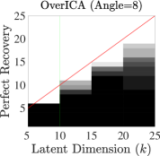
We expect that the optimal solution (if it exists and is unique) $B^{\ast}_{sdp}$ coincides with one of the atoms $d_{i}d_{i}^{\top}$ for some $i\in[k]$. This is not always the case, but we conjecture based on the experimental evidence that one of the atoms is recovered with high probability when $k\leq p^{2}/4$ (see Figure 1) and prove a weaker result (Theorem 2.1). The matrix $G\in\mathbb{R}^{p\times p}$ determines which of the atoms $d_{i}d_{i}^{\top}$ is the optimizer and its choice is discussed when we construct a deflation procedure (Section 2.4.3; see also Appendix C.1.4).

Intuition.

Since generalized covariances $H_{1}$,…,$H_{s}$ span the subspace $W$, the constraint set of (9) is:

$$\mathcal{K}:=\left\{B\in W:\mathrm{Tr}(B)=1,B\succeq 0\right\}.\vspace{-2mm}$$ (10)

It is not difficult to show (see Appendix C.2.2) that under Assumption 2.2 the atoms $d_{i}d_{i}^{\top}$ are extreme points of this set $\mathcal{K}$:

Lemma 2.4.1.

Let the atoms $d_{1}d_{1}^{\top}$, $d_{2}d_{2}^{\top}$, $\dots$, $d_{k}d_{k}^{\top}$ be linearly independent. Then they are extreme points of the set $\mathcal{K}$ defined in (10).

If the program (9) has a unique solution, the optimizer $B^{\ast}_{sdp}$ must be an extreme point due to the compactness of the convex set $\mathcal{K}$. If the set (10) does not have other extreme points except for the atoms $d_{i}d_{i}^{\top}$, $i\in[k]$, then the optimizer is guaranteed to be one of the atoms. This might not be the case if the set $\mathcal{K}$ contains extreme points different from the atoms. This might explain why the phase transition (at the rate $k\leq p^{2}/4$) happens and could potentially be related to the phenomenon of polyhedrality of spectrahedra (Bhardwaj et al., 2015).

Before diving into the analysis of this SDP, let us present its convex relaxation which enjoys certain desirable properties.

2.4.2 The Convex Relaxation

Let us rewrite (9) in an equivalent form. The constraint $B\in W:=\mathrm{Span}\left\{d_{1}d_{1}^{\top},\dots,d_{k}d_{k}^{\top}\right\}$ is equivalent to the fact that $B$ is orthogonal to any matrix from the orthogonal complement (null space) of $W$. Let the matrices $\left\{F_{1},F_{2},\dots,F_{m-k}\right\}$, where $m:=p(p+1)/2$, form a basis of the null space $\mathcal{N}(W)$. Then the program (9) takes an equivalent formulation:

$$B^{\ast}_{sdp}:= \mathop{\rm argmax}\limits_{B\in\mathcal{S}_{p}}\;\langle G,B\rangle$$ (11)

$$\langle B,F_{j}\rangle=0,\quad\text{for all}\quad j\in[m-k],$$

$$\mathrm{Tr}(B)=1,$$

$$B\succeq 0.$$

In the presence of (e.g., finite sample) noise, the subspace $W$ can only be estimated approximately (in the first step). Therefore, rather than keeping the hard first constraint, we introduce the relaxation

$$B^{\ast}:=\mathop{\rm argmax}\limits_{B\in\mathcal{S}_{p}} \;\langle G,B\rangle-\frac{\mu}{2}\sum_{j\in[m-k]}\langle B,F_{j}\rangle^{2}$$ (12)

$$\mathrm{Tr}(B)=1,\;B\succeq 0,$$

where $\mu>0$ is a regularization parameter which helps to adjust to an expected level of noise. Importantly, the relaxation (12) can be solved efficiently, e.g., via the fast iterative shrinkage-thresholding algorithm (FISTA; Beck and Teboulle, 2009) and the majorization-maximization principle (see, e.g., Hunter and Lange, 2004). See Appendix C.1 for details.

2.4.3 Deflation

The semi-definite program (9), or its relaxation (12), is designed to estimate only some one atom $d_{i}d_{i}^{\top}$. To estimate all other atoms we need a deflation procedure. In general, there is no easy and straightforward way to perform deflation in the overcomplete setting, but we discuss possible approaches below.

Clustering.

Since the matrix $G$ determines which atom is found, it is natural to repeatedly resample this matrix a multiple of $k$ times and then cluster the obtained atoms into $k$ clusters. This approach generally works well except in the cases where either (a) some of the atoms, say $d_{i}d_{i}^{\top}$ and $d_{j}d_{j}^{\top}$, are relatively close (e.g., in terms of angle in the space of all symmetric matrices) to each other, or (b) one or several atoms were not properly estimated. In the former case, one could increase the number of times $G$ is resampled, and the program is solved, but that might require very high number of repetitions. The latter issue is more difficult to fix since a single wrong atom could significantly perturb the overall outcome.

Adaptive Deflation.

Alternatively, one could adapt the constraint set iteratively to exclude from the search all the atoms found so far. For that, one can update the constraint set so that the subspace $W$ is replaced with the subspace that is spanned by all the atoms except for the ones which were already found. The most natural way to implement this is to add the found atoms to a basis of the null space of $W$, which is straightforward to implement with the relaxation (12). Similar to other deflation approaches, a poor estimate of an atom obtained in an earlier deflation step of such adaptive deflation can propagate this error leading to an overall poor result.

Semi-Adaptive Deflation.

We found that taking advantage of both presented deflation approaches leads to the best result in practice. In particular, we combine these approaches by first performing clustering and keeping only good clusters (with low variance over the cluster) and then continuing with the adaptive deflation approach. We assume this semi-adaptive deflation approach for all the experiments presented in Section 3.

2.4.4 Identifiability

In general, there are two types of identifiability of probabilistic models: (a) statistical and (b) algebraic. The statistical identifiability addresses whether the parameters of the model can be identified for given distributions. In particular, it is well known that the ICA model is not identifiable if (more than one of) the sources are Gaussian (Comon, 1994) and issues also arise when the sources are close to Gaussian (Sokol et al., 2014). These results also extend to the overcomplete case that we consider. However, we do not address these questions here and assume that the models we work with are statistically identifiable. Instead, we are interested whether our approach is algebraically identifiable, i.e., whether our algorithm correctly recovers the parameters of the model. In particular, we address the following question: When is the solution $B^{\ast}_{sdp}$ of the program (9) is one of the atoms $d_{i}d_{i}^{\top}$, $i\in[k]$?

We address this question in theory and in practice and focus on the population (infinite number of samples) case, where we assume that an exact estimate of the subspace $W$ is given and, therefore, one can use the representation $W:=\mathrm{Span}\left\{d_{1}d_{1}^{\top},\dots,d_{k}d_{k}^{\top}\right\}$ without loss of generality. Therefore, for the theoretical analysis purposes we assume that atoms $d_{i}d_{i}^{\top}$ are known, we consider the following program instead

$$B^{\ast}_{sdp}:= \mathop{\rm argmax}\limits_{B\in\mathcal{S}_{p}}\;\langle G,B\rangle$$ (13)

$$B\in\mathrm{Span}\left\{d_{1}d_{1}^{\top},d_{2}d_{2}^{\top},\dots,d_{k}d_{k}^{\top}\right\},$$

$$\mathrm{Tr}(B)=1,$$

$$B\succeq 0.$$

Phase Transition.

Figure 1: Phase transition of the program (13).

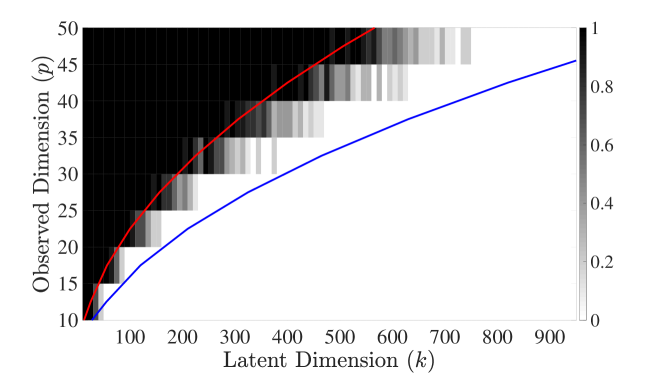
In Figure 1, we present the phase transition plot for the program (13) obtained by solving the program multiple times for different settings. In particular, for every pair $(p,k)$ we solve the program $n_{rep}:=50$ times and assign to the respective point the value equal to the fraction of successful solutions (where the optimizer was one of the atoms).

Given a fixed pair $(p,k)$, every instance of the program (13) is constructed as follows. We first sample a mixing matrix $D\in\mathbb{R}^{p\times k}$ so that every mixing component is from the standard normal distribution as described in Appendix D.1; and we sample a matrix $G\in\mathbb{R}^{p\times p}$ from the standard normal distribution. We then construct the constraint set of the program (13) by setting every matrix $H_{i}=d_{i}d_{i}^{\top}$ for all $i\in[k]$, where $s=k$. We solve every instance of this problem with the CVX toolbox (Grant et al., 2006) using the SeDuMi solver (Sturm, 1999).

We consider the observations dimensions $p$ from $10$ to $50$ with the interval of $5$ and we vary the number of atoms from $10$ to $1000$ with the interval of $10$. The resulting phase transition plots are presented in Figure 1. The blue line on this plot corresponds to the curve $k=p(p+1)/2$, which is the largest possible latent dimension of all symmetric matrices $\mathcal{S}_{p}$. The red line on this plot corresponds to the curve $k=p^{2}/4$. Since above the red line we observe 100% successful recovery (black), we conjecture that the phase transition happens around $k=p^{2}/4$.

Theoretical Results.

Interestingly, an equivalent conjecture, $k<p^{2}/4$, was made for the ellipsoid fitting problem (Saunderson et al., 2012, 2013) and the question remains open to our best knowledge. In fact, we show close relation between successful solution (recovery of an atom) of our program (13) and the ellipsoid fitting problem. In particular, a successful solution of our problem implies that the feasibility of its Lagrange dual program is equivalent to the ellipsoid fitting problem (see Appendix C.2.3). Moreover, using this connection, we prove the following:

Theorem 2.1.

Let $\varepsilon>0$. Consider a regime with $p$ tending to to infinity, and with $k$ varying according to the bound $k<(2-\varepsilon)p\log p$. As above, let the $d_{i}$ be random unit vectors and let $G=uu^{\top}$ for a random unit vector $u$. Then with high probability, the matrix $d_{i}d_{i}^{\top}$ for which $d_{i}^{\top}Gd_{i}$ is largest is the unique maximizer of the program (13).

Figure 2: A proof of concept in the asymptotic regime. See explanation in Section 3.1.

Figure 3: Comparison in the finite sample regime. See explanation in Section 3.2.

3 Experiments

It is difficult to objectively evaluate unsupervised learning algorithms on real data in the absence of ground truth parameters. Therefore, we first perform comparison on synthetic data. All our experiments can be reproduced with the publicly available code: https://github.com/anastasia-podosinnikova/oica.

3.1 Synthetic Data: Population Case

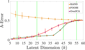
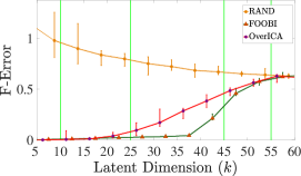
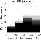
As a proof of concept, this simple experiment (Figure 2) imitates the infinite sample case. Given a ground truth mixing matrix $D$, we construct a basis of the subspace $W$ directly from the matrix $A:=D\odot D$ (see Appendix B.2). This leads to a noiseless estimate of the subspace. We then evaluate the performance of the second step of our OverICA algorithm and compare it with the second step of FOOBI. We fix the observed dimension $p=10$ and vary the latent dimension from $k=5$ to $k=60$ in steps of $5$. For every pair $(p,k)$, we repeat the experiment $n_{rep}=10$ times and display the minimum, median, and maximum values. Each time we sample the mixing matrix $D$ with mixing components from the standard normal distribution (see Appendix D.1.1). Note that we tried different sampling methods and distributions of the mixing components, but did not observe any significant difference in the overall result. See Appendix D.1.2 for further details on this sampling procedure.

The error metrics (formally defined in Appendix D.2) are: (a) f-error is essentially the relative Frobenius norm of the mixing matrices with properly permuted mixing components (lower is better); (b) a-error measures the angle deviations of the estimated mixing components vs the ground truth (lower is better); and (c) “perfect” recovery rates, which show for every $i\in[k]$ the fraction of perfectly estimated $i$ components. We say that a mixing component is “perfectly” recovered if the cosine of the angle between this component $d_{i}$ and its ground truth equivalent $d_{\pi(i)}$ is at least $0.99$, i.e., $\cos(d_{i},\widehat{d}_{\pi(i)})\geq 0.99$. Note that the respective angle is approximately equal to 8. Then the black-and-white perfect recovery plots (in Figure 2) show if $i\leq k$ (on the y-axis) components were perfectly recovered (black) for the given latent dimension $k$ (x-axis). These black vertical bars cannot exceed the red line $i=k$, but the closer they approach this line, the better. The vertical green lines correspond to $k=p=10$, $k=p^{2}/4=25$, $k=p(p-1)/2$, and $k=p(p+1)/2$. Importantly, we see that OverICA works better or comparably to FOOBI in the regime $k<p^{2}/4$. Performance of OverICA starts to deteriorate near the regime $k\approx p^{2}/4$ and beyond, which is in accord with our theoretical results in Section 2.4.4. Note that to see whether the algorithms work better than random, we display the errors of a randomly sampled mixing matrix (RAND; see Appendix D.1.1).

3.2 Synthetic Data: Finite Sample Case

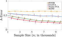
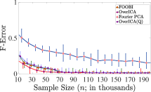
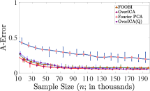
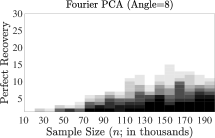
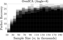
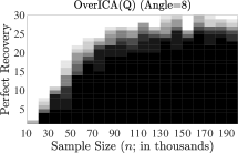
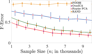
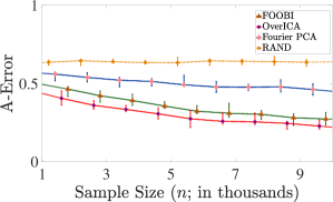
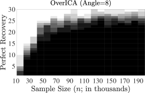
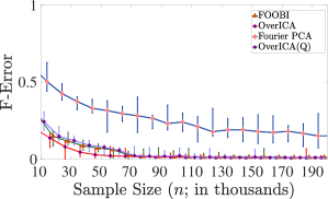
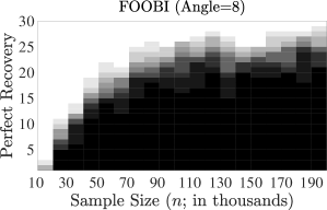
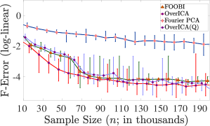
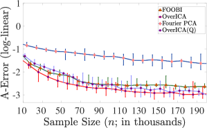
With these synthetic data we evaluate performance of overcomplete ICA algorithms in the presence of finite sample noise but absence of model misspecification. In particular, we sample synthetic data in the observed dimension $p=15$ from the ICA model with uniformly distributed (on $[-0.5,0.5]$) $k=30$ sources for different sample sizes $n$ taking values from $n=1,000$ to $n=10,000$ in steps of $1,000$ (two left most plots in the top line of Figure 3) and values from $n=10,000$ to $n=210,000$ in steps of $10,000$ (two right most plots in the top line of Figure 3; see also Figure 6 in Appendix for log-linear scale). Note that the choice of dimensions $p=15$ and $k=30$ corresponds to the regime $k<p^{2}/4\approx 56$ of our guarantees. We repeat the experiment $n_{rep}:=10$ times for every $n$ where we every time resample the (ground truth) mixing matrix (with the sampling procedure described in Appendix D.1.1). See further explanation in Appendix D.1.3.

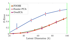
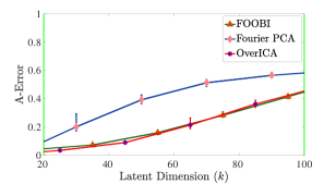
We compare the Fourier PCA algorithm (Goyal et al., 2014), the FOOBI algorithm (De Lathauwer et al., 2007), OverICA from Algorithm 1, and a version of the OverICA algorithm where the first step is replaced with the construction based on the fourth-order cumulant, a.k.a. quadricovariance (OverICA(Q); see Appendix B.2). Note that we can not compare with the reconstruction ICA algorithm by Le et al. (2011) because it estimates the de-mixing (instead of mixing) matrix. Similarly to Section 3.1, we measure the Frobenius error (f-error), the angle error (a-error), and the perfect recovery for the angle of $8$. We observe that the generalized covariance-based OverICA algorithm performs slightly better which we believe is due to the lower sample complexity. Fourier PCA on the contrary performs with larger error, which is probably due to the higher sample complexity and larger noise resulting from estimation using fourth-order generalized cumulants.

Table 1: Computational complexities ($n$ is the sample size, $p$ is the observed dimension, $k$ is the latent dimension, $s$ is the number of generalized covariances, usually $s=O(k)$).

Procedure	Memory	Time
GenCov	$O(p^{2}s)$	$O(snp^{2})$
CUM	$O(p^{4})$	$O(np^{4}+k^{2}p^{2})$
FOOBI	$O(p^{4}k^{2}+k^{4})$	$O(np^{4}+k^{2}p^{4}+k^{6})$
OverICA	$O(sp^{2})$	$O(nsp^{2})$
OverICA(Q)	$O(p^{4})$	$O(np^{4}+k^{2}p^{2})$
Fourier PCA	$O(p^{4})$	$O(np^{4})$

3.3 Computational Complexities

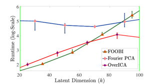
In Table 1, we summarize the timespace complexities of the considered overcomplete ICA algorithms and two sub-procedures they use: generalized covariances (GenCov; used by OverICA) from Section 2.3 and the forth-order cumulant (CUM; used by OverICA(Q) and FOOBI; see Appendix B.2) (see Appendix D.3). Importantly, we can see that our OverICA algorithm has a significantly lower complexity. In Appendix D.3, we present runtime comparisons of these algorithms.

3.4 Real Data: CIFAR-10 Patches

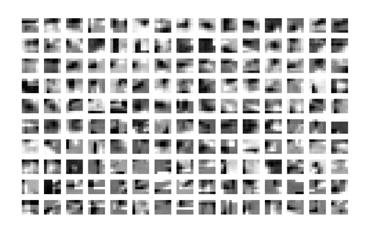
Finally, we estimate the overcomplete mixing matrix of data formed of patches of the CIFAR-10 dataset (see, e.g., Krizhevsky et al., 2014). In particular, we transform the images into greyscale and then form $7$-by-$7$ patches for every interior point (at least 3 pixels from the boundary) of every image from the training batch 1 of the CIFAR-10 dataset. This results in $6,760,000$ patches each of dimension $p=49$. We perform the estimation of the mixing matrix for $k=150$ latent mixing components. The resulting atoms are presented in Figure 4. Note that since ICA is scale (and therefore sign) invariant, the sign of every component can be arbitrary flipped. We present the obtained components in the scale where black and white corresponds to the extreme positive or negative values and we observe that these peaks are concentrated in rather pointed areas (which is a desirable property of latent components). Note that the runtime of this whole procedure was around $2$ hours on a laptop. Due to high timespace complexities (see Section 3.3), we cannot perform similar estimation neither with FOOBI nor with Fourier PCA algorithms.

Figure 4: Mixing components obtained from $7$-by-$7$ patches, i.e., $p=49$, of the CIFAR-10 dataset ($k=150$, i.e., overcomplete). ICA does not preserve non-negativity and the signs of ICA mixing components can be arbitrarily flipped due to the scaling unidentifiability; here black and white correspond to the extreme positive and extreme negative values. The colorbar limits of every image are the same and the signs are alligned to have positive scalar product with the first component.

4 Conclusion

We presented a novel ICA algorithm for estimation of the latent overcomplete mixing matrix. Our algorithm also works in the (under-)complete setting, enjoys lower computational complexity, and comes with theoretical guarantees, which is also confirmed by experiments.

Appendix A Apendix: Technical Details

A.1 Matricization and Vectorization

One can vectorize a matrix by stacking its columns and one can matricize a vector by performing the reverse of the vectorization operation. Below we formalize these notions.

A.1.1 Vectorization

Given a matrix $X\in\mathbb{R}^{m\times n}$, we define its vectorization as $x:=\mathrm{vec}(X)\in\mathbb{R}^{mn}$ such that

$$x_{(i-1)m+j}:=X_{ij},\quad\text{for all}\quad i\in[m],\;j\in[n].$$ (14)

We also use in this paper the fact that the vectorization of a rank matrix $X:=ab^{\top}$ is equal to the Khatri-Rao product (See Appendix A.2) of the vectors $a$ and $b$, i.e.,

$$\mathrm{vec}(ab^{\top})=a\odot b.$$ (15)

A.1.2 Matricization

We define the matricization operation as the inverse of the vectorization operation, i.e. the matricization of a vector $x\in\mathbb{R}^{mn}$ is a matrix $X:=\mathrm{mat}(x)\in\mathbb{R}^{m\times n}$ such that

$$X_{ij}:=x_{(i-1)m+j},\quad\text{for all}\quad i\in[m],\;j\in[n].$$ (16)

A.2 The Kharti-Rao Product

The Khatri-Rao product of two matrices $A\in\mathbb{R}^{n\times k}$ and $B\in\mathbb{R}^{m\times k}$, with columns $b_{j}$, for $j\in[k]$, is an $(nm\times k)$-matrix $A\odot B$ of the form:

$$A\odot B:=\begin{pmatrix}A_{11}b_{1}&A_{12}b_{2}&\dots&A_{1k}b_{k}\\ A_{21}b_{1}&A_{22}b_{2}&\dots&A_{2k}b_{k}\\ A_{31}b_{1}&A_{32}b_{2}&\dots&A_{3k}b_{k}\\ \dots&\dots&\dots&\dots\\ A_{n1}b_{1}&A_{n2}b_{2}&\dots&A_{nk}b_{k}\end{pmatrix}.$$ (17)

Note that although the Khatri-Rao product of two vectors coincide with the Kronecker product of these vectors, the two products are different in general.

Moreover, as we mentioned in Appendix A.1, the vectorization of a rank-1 matrix is equal to the Khatri-Rao product of respective vectors.

Appendix B Apendix: Independent Component Analysis

B.1 The Fourth-Order Cumulant and Kurtosis

B.1.1 The Fourth-Order Cumulant

Given a $p$-valued zero-mean random vector $x$, its fourth-order cumulant is the symmetric $(p\times p\times p\times p)$-tensor $\mathcal{C}_{x}$ such that

$${[\mathcal{C}_{x}^{(4)}]}{}_{i_{1}i_{2}i_{3}i_{4}}:=\mathrm{cum}[x_{i_{1}},x_{i_{2}},x_{i_{3}},x_{i_{4}}]$$ (18)

$$:=\mathbb{E}[x_{i_{1}}x_{i_{2}}x_{i_{3}}x_{i_{4}}]-\mathbb{E}[x_{i_{1}}x_{i_{2}}]\mathbb{E}[x_{i_{3}}x_{i_{4}}]$$

$$-\mathbb{E}[x_{i_{1}}x_{i_{3}}]\mathbb{E}[x_{i_{2}}x_{i_{4}}]-\mathbb{E}[x_{i_{1}}x_{i_{4}}]\mathbb{E}[x_{i_{2}}x_{i_{4}}].$$

If $x$ is not zero-mean, this definition is instead applied to the variable $\tilde{x}:=x-\mathbb{E}(x)$.

B.1.2 Kurtosis

The kurtosis of a univariate zero-mean random variable $\alpha$ is the number $\kappa_{\alpha}$ such that

$$\kappa_{\alpha}:=\mathrm{cum}[\alpha,\alpha,\alpha,\alpha]=\mathbb{E}[\alpha^{4}]-3\mathbb{E}[\alpha^{2}]\mathbb{E}[\alpha^{2}].$$ (19)

Note that:

• If $\alpha$ is from the standard normal distribution then $\kappa_{\alpha}=0$;

• If $\alpha$ is from the uniform distribution such that $\mathbb{E}(\alpha)=0$ and $\mathrm{var}(\alpha)=1$ then $\kappa_{\alpha}=-1.2$;

• If $\alpha$ is from the Laplace distribution such that $\mathbb{E}(\alpha)=0$ and $\mathrm{var}(\alpha)=1$ then $\kappa_{\alpha}=3$.

B.2 The Fourth-Order Cumulant of the ICA Model

In this section, we recall the form of the fourth-order cumulant of the ICA model originally utilized by De Lathauwer et al. (2007) for the FOOBI algorithm. This cumulant can be used for the construction of subspace $W$ as an alternative to the procedure presented in Section 2.3.

The formal definition of the fourth-order cumulant can be found in Appendix B.1.1. By the multi-linearity and independence properties of cummulants (see, e.g., Comon and Jutten, 2010, Chapter 5), the fourth-order cumulant of the ICA model (1) is the tensor

$$\mathcal{C}_{x}^{(4)}=\sum_{i=1}^{k}\kappa_{\alpha_{i}}d_{i}\otimes d_{i}\otimes d_{i}\otimes d_{i},$$

where $\otimes$ stands for the outer product and $\kappa_{\alpha_{i}}$ is the kurtosis of the $i$-th source (see Appendix B.1.2 for the definition). As De Lathauwer et al. (2007) show, the flattening of this tensor is a matrix $C\in\mathbb{R}^{p^{2}\times p^{2}}$ such that

$$C=(D\odot D)\mathrm{Diag}(\kappa)(D\odot D)^{\top},$$ (20)

where $\odot$ stands for the Khatri-Rao product (recall the definition is Appendix A.2) and the $i$-th element of the vector $\kappa\in\mathbb{R}^{k}$ is the kurtosis $\kappa_{\alpha_{i}}$ of the $i$-th source $\alpha_{i}$.

This expression (20) is the key for the subspace construction. To see that, let us have a look at the matrix $A\in\mathbb{R}^{p^{2}\times k}$ such that

$$A:=D\odot D.$$ (21)

The $i$-th column of this matrix $a_{i}:=A_{:,i}=d_{i}\odot d_{i}$ and its matricization $A_{i}:=\mathrm{mat}(a_{i})=\mathrm{mat}(d_{i}\odot d_{i})=d_{i}d_{i}^{\top}$ is equal to the $i$-th atom. Therefore, using this flattening-matricization trick one can easily obtain an estimate of the subspace $W$. Indeed, a basis of $W$ can be constructed as a matricization of a basis of the column space of $C$. The latter can be obtained, e.g., via the eigen decomposition or singular value decomposition of $C$. In particular, let $C=U\Sigma V$ be the SVD of $C$. Then a basis of the subspace $W$ can be constructed as $H_{i}:=\mathrm{mat}(u_{i})$ for every $i\in[k]$, where $u_{i}$ is the $i$-th left singular vector, and it holds that

$$W=\mathrm{Span}\left\{\mathrm{mat}(u_{1}),\dots,\mathrm{mat}(u_{k})\right\}.$$ (22)

This exact construction is used in a practical implementation of the FOOBI algorithm and can be used as a replacement of the Step I in the OverICA Algorithm 1.

Appendix C The Semi-Definite Program

C.1 Algorithm for the Relaxation (12)

This section applies the FISTA algorithm by Beck and Teboulle (2009) for finding the solution of the convex relaxation (12).

C.1.1 FISTA

Let $\mathcal{K}$ be a set of all symmetric PSD matrices with unit trace, i.e. $\mathcal{K}:=\left\{B\in\mathcal{S}_{p}:B\succeq 0,\mathrm{Tr}(B)=1\right\}$, where $\mathcal{S}_{p}$ denotes the set of all symmetric matrices in $\mathbb{R}^{p\times p}$. Let $g(B):=\iota_{\mathcal{K}}(B)$ be the indicator function of the set $\mathcal{K}$ and let the negative objective of the problem (12) be

$$f(B):=-\langle G,B\rangle+\frac{\mu}{2}\sum_{j\in[m-k+t]}\langle B,F_{j}\rangle^{2}.$$

We then can solve the problem

$$\mathop{\rm min}\limits_{B\in\mathbb{R}^{p\times p}}f(B)+g(B)$$

with FISTA Beck and Teboulle (2009). The gradient of the differentiable part of the objective is

$$\nabla f(B)=-G^{\top}+\mu\sum_{j\in[m-k+t]}\mathrm{Tr}(F_{j}B)F_{j}^{\top},$$

where we used the fact that its Lipschitz constant is $L=\mu$. This is summarized in Algorithm 2. The projection on $\mathcal{K}$ can be computed roughly in $O(p^{3})$ time (see Section C.1.2).

Algorithm 2 FISTA for (12)

1:Input: $Y^{(1)}=B^{(0)}\in\mathcal{S}_{p}$, $z_{1}=1$

2:while not converged or $n>n_{max}$ do

3:   $B^{(n)}=\mathrm{Proj}_{\mathcal{K}}\left[Y^{(n)}-\frac{1}{L}\nabla f(Y^{(n)})\right]$

4:   $z_{n+1}=\frac{1}{2}\left(1+\sqrt{1+4z_{n}^{2}}\right)$

5:   $Y^{(n+1)}=B^{(n)}+\left(\frac{z_{n}-1}{z_{n+1}}\right)(B^{(n)}-B^{(n-1)})$

6:   $n\leftarrow n+1$

7:end while

8:Output: $B^{\ast}=B^{(n)}$

C.1.2 Projection onto $\boldsymbol{\mathcal{K}}$

The projection onto the set $\mathcal{K}:=\left\{B\in\mathcal{S}_{p}:B\succeq 0,\mathrm{Tr}(B)=1\right\}$ of a symmetric matrix $B$ can be computed by first computing the eigendecomposition of this matrix $B=V\Lambda V^{\top}$ and then projecting its eigenvalues $\lambda=\mathrm{Diag}(\Lambda)$ onto the probability simplex $\Delta_{p}$. Then the projection is obtained as $\mathrm{Proj}_{\mathcal{K}}(B)=V\mathrm{Diag}[\mathrm{Proj}_{\Delta_{p}}(\lambda)]V^{\top}$. Note that the probability simplex is defined as $\Delta_{p}:=\left\{x\in\mathbb{R}^{p}:\|x\|_{1}=1,x\succcurlyeq 0\right\}$ and the projection onto the probability simplex can be computed in linear time (see, e.g., Duchi et al., 2008).

C.1.3 Majorization-Minimization

We observe in practice that our problem benefits significantly from the majorization-minimization approach (see, e.g., Hunter and Lange, 2004), i.e. earlier stopping of the procedure in Algorithm 2 and restarting it again with a matrix $B^{(0)}_{next}$ obtained from the largest eigenvector of the matrix $B^{\ast}_{prev}$. We experimentally found that performing rather large number of majorization minimization steps (e.g., approx. 50) but with the relatively small maximal number of iterations $n_{max}=100$ gives the best experimental performance in terms of convergence speed and runtime. In particular, this is the setting we used for the experiments presented in Section 3.

C.1.4 The Choice of $G$

The choice of the matrix $G$ is an important part of our deflation procedure. We found experimentally that choosing $G$ that belongs to the subspace $W^{(t)}$ is beneficial. The latter is also without loss of generality, since if $G$ has a component that does not belong to the subspace, the inner product $\langle G,B\rangle$ of the objective would not be affected by that part as it would be orthogonal to $B$.

In particular, let $F^{(t)}:=\{f_{j}^{(t)},j\in[m-k+t]\}$, where $f_{j}^{(t)}:=\mathrm{vec}(F_{j}^{(t)})$, be a basis of the orthogonal complement at the $t$-th deflation step. Let $H^{(t)}:=\{h_{i}^{(t)},i\in[k-t]\}$ be a basis of the orthogonal complement of $F^{(t)}$, i.e. a basis of $W^{(t)}$. Let $u^{(t)}$ be the first left singular vector of $H^{(t)}$, then we set $G^{(t)}:=u^{(t)}u^{(t)\top}$.

C.2 Theory

We first recall the ellipsoid fitting problem and results related to the proof of our main Theorem 2.1. Note that we also prove slightly stronger result for the ellipsoid fitting problem in Theorem C.2.

We then proceed as follows. In Appendix C.2.2, we prove Lemma 2.4.1 about extreme points of the constraint set of the program (13). Then, in Appendix C.2.3, we derive the dual of the program (13) and show its close relation to the ellipsoid fitting problem. Finally, in Appendix C.2.4, we prove Theoremthm:main by constructing a appropriate ellipsoid.

C.2.1 Ellipsoid Fitting

Ellipsoid fitting is the following elementary geometric question: given $k$ points $v_{1},\ldots,v_{k}\in\mathbb{R}^{p}$, does there exist an ellipsoid passing exactly through them? That is, does there exist a matrix $Y\succeq 0$ with $v_{i}^{\top}Yv_{i}=1$?

We consider this problem in an average-case regime in which $p\to\infty$ and the $v_{i}$ are chosen independently from some distribution. Saunderson et al. (2013) considers the case where the $v_{i}$ are standard Gaussians, and obtains the following:

Theorem C.1 (Saunderson et al. (2013)).

Suppose $k\leq p^{6/5-\varepsilon}$ for some fixed $\varepsilon>0$. Then with very high probability over $v_{1},\ldots,v_{k}\in\mathbb{R}^{p}$ drawn independently from $\mathcal{N}(0,I)$, there exists an ellipsoid passing through those points.

The same paper conjectures based on empirical evidence that ellipsoid fitting in this average-case model is possible when $k<p^{2}/4$, exhibiting a sharp threshold phenomenon. To our knowledge, this question remains open.

Our first result is a slight generalization of the above which allows for small perturbations in the norm of the vectors. We will need this result later for the SDP analysis for ICA.

Theorem C.2.

Let $w_{1},\ldots,w_{k}\in\mathbb{R}^{p}$ be drawn independently from $\mathcal{N}(0,I)$. Let $v_{i}=\pi_{i}w_{i}$ where each $\pi_{i}$ is a scalar random variable satisfying the following: for any $\delta>0$, $|1/\pi_{i}^{2}-1|\leq p^{-1/2+\delta}$ with very high probability. (The $\pi_{i}$ need not be identically distributed nor independent from $w_{i}$ or each other.) Suppose $k\leq p^{6/5-\varepsilon}$ for some fixed $\varepsilon>0$. Then with very high probability there exists an ellipsoid passing through $v_{1},\ldots,v_{k}$.

The rest of this section is devoted to the proof of this theorem. The proof uses many ideas from Saunderson et al. (2013).

We will construct our ellipsoid $Y$ in the form

$$Y=I/p+\sum_{j=1}^{k}\beta_{j}w_{j}w_{j}^{\top},$$

for some scalars $\beta_{j}$. We wish to satisfy constraints $v_{i}^{\top}Yv_{i}=1$, i.e.

$$\pi_{i}^{2}\|w_{i}\|^{2}/p+\pi_{i}^{2}\sum_{j}\beta_{j}\langle w_{i},w_{j}\rangle^{2}=1,$$

which can be re-written as

$$\sum_{j}\beta_{j}\langle w_{i},w_{j}\rangle^{2}=\frac{1}{\pi_{i}^{2}}-\frac{1}{p}\|w_{i}\|^{2}.$$

This is a linear system $V\beta=h$ where $V_{ij}=\langle w_{i},w_{j}\rangle^{2}$ and $h_{i}=1/\pi_{i}^{2}-\|w_{i}\|^{2}/p$. Therefore we take $\beta=V^{-1}h$.

The linear operator $\mathcal{A}^{\dagger}$ that takes the vector $h$ to the matrix $\sum_{j=1}^{k}\beta_{j}w_{j}w_{j}^{\top}$ (with $\beta=V^{-1}h$) is studied in Saunderson et al. (2013) (with some proofs deferred to Saunderson (2011)), where the following bound is shown on the “infinity-to-spectral” norm.

Proposition C.1 (Saunderson et al. (2013), Proposition 3).

If $p=o(k)$ and $k=o(p^{4/3})$ then

$$\|\mathcal{A}^{\dagger}\|_{\infty\to\mathrm{sp}}\leq O(k^{5/4}p^{-2})$$

with very high probability over $\{w_{i}\}$.

The requirement $p=o(k)$ does not concern us because it is sufficient to prove Theorem C.2 in the case $p=o(k)$; this is because decreasing $k$ only makes it easier to fit an ellipsoid through $k$ points.

Our goal is to show $Y\succeq 0$ so it is sufficient to show $\|A^{\dagger}h\|\leq 1/p$, which we will do using $\|\mathcal{A}^{\dagger}h\|\leq\|\mathcal{A}^{\dagger}\|_{\infty\to\mathrm{sp}}\|h\|_{\infty}$. It remains to bound $\|h\|_{\infty}$.

Let $\delta>0$, to be chosen later. Recall that $h_{i}=1/\pi_{i}^{2}-\|w_{i}\|^{2}/p$. To control the first term, we have by assumption that with very high probability, $|1/\pi_{i}^{2}-1|\leq p^{-1/2+\delta}$ for all $i$. Note that $\|w_{i}\|^{2}\sim\chi_{p}^{2}$. We will use the following chi-squared tail bound.

Lemma C.2.1 (Saunderson (2011), Lemma 7).

$$\operatorname{\Pr}[|\chi_{p}^{2}-p|\geq t]\leq 2\exp\left(-\frac{1}{8}\mathop{\rm min}\limits\left\{\frac{t^{2}}{p},t\right\}\right).$$

This implies that $\left|\|w_{i}\|^{2}/p-1\right|\leq p^{-1/2+\delta}$ with very high probability. Therefore $\|h\|_{\infty}\leq 2p^{-1/2+\delta}$ with very high probability. To complete the proof of Theorem C.2, we have, using the assumption $k\leq p^{6/5-\varepsilon}$,

$$\|\mathcal{A}^{\dagger}h\| \leq\|\mathcal{A}^{\dagger}\|_{\infty\to\mathrm{sp}}\|h\|_{\infty}\leq O(k^{5/4}p^{-2}\cdot p^{-1/2+\delta})$$

$$\leq O(p^{5/4(6/5-\varepsilon)-5/2+\delta})=O(p^{-1-5\varepsilon/4+\delta}),$$

which is less than $1/p$ for sufficiently large $p$, provided we choose $\delta$ small enough.

C.2.2 Proof of Lemma 2.4.1

In this section, we prove Lemma 2.4.1. Recall that Lemma 2.4.1 states that: if the atoms $d_{1}d_{1}^{\top}$, $d_{2}d_{2}^{\top}$, $\dots$, $d_{k}d_{k}^{\top}$ are linearly independent, then they are extreme points of the set $\mathcal{K}$ defined in (10).

Proof.

An extreme point of a convex set cannot be expressed as a convex combination of any two points from this set. Assume that an atom $d_{j}d_{j}^{\top}$, for some $j\in[k]$, can be expressed as $d_{j}d_{j}^{\top}=\lambda A+(1-\lambda)B$, where $A,B\in\mathcal{K}$ and $\lambda\in[0,1]$. Since $A,B\in W$, there exist vectors $\alpha\in\mathbb{R}^{k}$ and $\beta\in\mathbb{R}^{k}$ such that $A=\sum_{i=1}^{k}\alpha_{i}d_{i}d_{i}^{\top}$ and $B=\sum_{i=1}^{k}\beta_{i}d_{i}d_{i}^{\top}$. Therefore,

$$d_{j}d_{j}^{\top}=\sum_{i=1}^{k}[\lambda\alpha_{i}+(1-\lambda)\beta_{i}]d_{i}d_{i}^{\top}.$$

This, however, contradicts to the linear independence of the matrices $d_{1}d_{1}^{\top}$, …, $d_{k}d_{k}^{\top}$. Note that every atom belongs to the set $\mathcal{K}$. Indeed, every atom $d_{i}d_{i}^{\top}$ is a positive semi-definite matrix by definition and it has unit trace by Assumption 2.1. ∎

C.2.3 The Dual

In this section, we derive the dual of the program (13). The first constraint, $B\in\mathrm{Span}\left\{d_{1}d_{1}^{\top},d_{2}d_{2}^{\top},\dots,d_{k}d_{k}^{\top}\right\}$, is equivalent to $B=\sum_{i=1}^{k}\beta_{i}d_{i}d_{i}^{\top}$ for some $\beta\in\mathbb{R}^{k}$ and one gets an equivalent to (13) program

$$\beta^{\ast}:= \mathop{\rm argmin}\limits_{\beta\in\mathbb{R}^{k}}\;-\sum_{i=1}^{k}\beta_{i}d_{i}^{\top}Gd_{i}$$ (23)

$$\sum_{i=1}^{k}\beta_{i}d_{i}d_{i}^{\top}\succeq 0,$$

$$\sum_{i=1}^{k}\beta_{i}=1,$$

where the last constraint is obtained from $\mathrm{Tr}(B)=1$ and Assumption 2.1. The original variable $B^{\ast}_{sdp}$ is then obtained as $B^{\ast}_{sdp}=\sum_{i=1}^{k}\beta^{\ast}_{i}d_{i}d_{i}^{\top}$. The Lagrangian of this problem is

$$\mathcal{L}(\beta;\;\lambda,Z) =\lambda\left(\sum_{i=1}^{k}\beta_{i}-1\right)-\langle Z,\sum_{i=1}^{k}\beta_{i}d_{i}d_{i}^{\top}\rangle-\sum_{i=1}^{k}\beta_{i}d_{i}d_{i}^{\top}$$ (24)

$$=\sum_{i=1}^{k}\left[\beta_{i}\langle d_{i}d_{i}^{\top},\lambda I-G-Z\rangle\right]-\lambda,$$

where $\lambda\in\mathbb{R}$ and $Z\succeq 0$ are the Lagrange dual variables. The Lagrangian is linear in $\beta$ and its infimum is finite only if $\langle d_{i}d_{i}^{\top},\lambda I-G-Z\rangle=0$ for all $i\in[k]$. Therefore, the dual problem takes the form

$$\mathop{\rm maximize}\limits_{\lambda\in\mathbb{R},Z\succeq 0}\;-\lambda$$ (25)

$$\lambda\left\|d_{i}\right\|_{2}^{2}-d_{i}^{\top}Gd_{i}=d_{i}^{\top}Zd_{i},\quad\text{for all}\quad i\in[k].$$

The following lemma is then follows.

Lemma C.2.2.

An atom $d_{j}d_{j}^{\top}$ for some $j\in[k]$ is the optimizer of the program (13) if and only if there exists a $Z\succeq 0$ such that

$$d_{i}^{\top}Zd_{i}=d_{j}^{\top}Gd_{j}\left\|d_{i}\right\|_{2}^{2}-d_{i}^{\top}Gd_{i},\quad i\in[k],i\neq j.$$ (26)

Proof.

One of the atoms $d_{j}d_{j}^{\top}$ is an optimizer of the primal problem (13) if and only if the optimizer of the equivalent program (23) is a $\beta$ such that $\beta_{j}=1$ and $\beta_{i}=0$ for all $i\in[k]$ and $i\neq j$. Let the dual problem (25) be feasible. Then, since the relative interior of the program (23) is non-empty, the strong duality holds. Therefore, the optimal value of $\lambda$ must be $\lambda=d_{j}^{\top}Gd_{j}$ and then the dual is feasible if and only if $d_{i}^{\top}Zd_{i}=d_{j}^{\top}Gd_{j}\left\|d_{i}\right\|_{2}^{2}-d_{i}^{\top}Gd_{i}$ for every $i\in[k]$ and $i\neq j$. ∎

In Appendix C.2.4, we construct such an ellipsoid in order to prove our main identifiability result.

C.2.4 Proof of Main Theorem 2.1

In this section, we prove our main theoretical result stated in Theorem 2.1 that provides identifiability results for the program (13). For convenience, we recall the problem formulation.

Let the vectors $d_{1},\ldots,d_{k}$ be drawn i.i.d. from the unit sphere in $\mathbb{R}^{p}$. We wish to recover the atoms $d_{i}d_{i}^{\top}$ from the subspace $\mathrm{span}\{d_{i}d_{i}^{\top}\}\subset\mathbb{R}^{p\times p}$. To this end, we consider the following SDP:

Program C.3.

maximize $$\langle G,B\rangle$$

subject to $$B\succeq 0,$$

$$\mathrm{Tr}(B)=1,$$

$$B\in\mathrm{span}\{d_{i}d_{i}^{\top}\}.$$

Here $G\in\mathbb{R}^{p\times p}$ is some objective matrix, to be chosen randomly from some ensemble.

We are interested in understanding the performance of this SDP, when the objective $G$ is chosen as a random rank-one matrix, i.e. as $uu^{\top}$ for a vector $u$ drawn uniformly from the unit sphere in $\mathbb{R}^{p}$ (independently from $\{d_{i}\}$). Our main result is the following:

Theorem (Theorem 2.1).

Let $\varepsilon>0$. Consider a regime with $p$ tending to to infinity, and with $k$ varying according to the bound $k<(2-\varepsilon)p\log p$. As above, let the $d_{i}$ be random unit vectors and let $G=uu^{\top}$ for a random unit vector $u$. Then with high probability, the matrix $d_{i}d_{i}^{\top}$ for which $d_{i}^{\top}Gd_{i}$ is largest is the unique maximizer of Program C.3.

The rest of this section is devoted to proving this theorem. Throughout the proof, it will be convenient to consider the following equivalent formulation of Program C.3.

Program C.4.

maximize $$\sum_{i=1}^{k}c_{i}\alpha_{i}$$

subject to $$B\triangleq(1+\alpha_{1})d_{1}d_{1}^{\top}+\sum_{i>1}\alpha_{i}d_{i}d_{i}^{\top}\succeq 0,$$

$$\sum_{i=1}^{k}\alpha_{i}=0,$$

where $c_{i}=d_{i}^{\top}Gd_{i}=\langle u,d_{i}\rangle^{2}$ and we have re-indexed the $d_{i}$ such that $d_{i}^{\top}Gd_{i}$ are in decreasing order (so that $d_{1}d_{1}^{\top}$ is the matrix we hope to recover). Our goal is to prove that $\alpha=0$ is the unique optimal solution to Program C.4. (The objective values of Programs C.3 and C.4 differ by an additive constant but this has no effect on the argmax.)

First sample the random vector $u$. Since the norm of $u$ does not affect the argmax of the SDP, we can take (for convenience) $u$ to be a uniformly random vector of norm $\sqrt{p}$. By a change of basis we can assume without loss of generality that $u=\sqrt{p}e_{1}$ where $e_{1}$ is the first standard basis vector.

Next sample the first coordinate $(d_{i})_{1}$ of each $d_{i}$ and let $c_{i}=\langle u,d_{i}\rangle^{2}=p(d_{i})_{1}^{2}$. Re-index so that the $c_{i}$ are in decreasing order. A typical $c=(c_{1},\ldots,c_{k})$ has the following properties.

Lemma C.2.3.

Let $\eta>0$. With high probability, $c$ satisfies

1. $(2-\eta)\log k\leq c_{2}\leq c_{1}\leq(2+\eta)\log k$,

2. $1-\eta\leq\frac{1}{k}\sum_{i}c_{i}\leq 1+\eta$,

3. $c_{k}\geq\frac{1}{k\log k}$, and

4. $c_{1}-c_{2}\geq\frac{1}{k^{2}\log k}$.

Recall that we have indexed so that $c_{1}\geq c_{2}\geq\cdots\geq c_{k}$.

Proof.

The $c_{i}$ are independent and each is distributed as $p\,g_{1}^{2}/(\sum_{j=1}^{p}g_{j}^{2})$ where $g_{j}\sim\mathcal{N}(0,1/p)$. By the Chernoff bound we have for any $\eta>0$,

$$\operatorname{\Pr}\left[\sum_{j=1}^{p}g_{j}^{2}\leq 1-\eta\right]\leq((1-\eta)e^{\eta})^{p/2},$$

$$\operatorname{\Pr}\left[\sum_{j=1}^{p}g_{j}^{2}\geq 1+\eta\right]\leq((1+\eta)e^{-\eta})^{p/2}.$$

By a union bound over the $k$ indices we have with high probability that for every $c_{i}$, $1-\eta\leq\sum_{j=1}^{p}g_{j}^{2}\leq 1+\eta$. It is therefore sufficient to prove (i), (ii), (iii) in the case where the $c_{i}$ are i.i.d. distributed as $p\,g_{1}^{2}\sim\chi_{1}^{2}$. (i) follows from well-known results on order statistics of i.i.d. Gaussians (see e.g. Bovier (2005)). (ii) follows by the Chernoff bound. To prove (iii), note that since the $\chi_{1}^{2}$ PDF is bounded above by a constant $C$, we have $\operatorname{\Pr}[\chi_{1}^{2}\leq r]\leq Cr$; now take a union bound over all $k$ and set $r=1/(k\log k)$.

To prove (iv) we will prove the stronger statement that no two entries of $c_{i}$ are within distance $1/(k^{2}\log k)$ of each other. Fix a pair $i,j$ with $i\neq j$ and fix any value for $c_{i}$. The PDF of the distribution of $c_{j}$ is bounded above by a constant $C$ (uniformly over all $p$), so we have $\operatorname{\Pr}[|c_{i}-c_{j}|\leq r]\leq 2Cr$ over the randomness of $c_{j}$. The proof now follows by setting $r=1/(k^{2}\log k)$ and taking a union bound over all ${k\choose 2}$ pairs of indices. ∎

From this point onward we will fix a vector $c$ satisfying the conclusion of Lemma C.2.3 (for some $\eta$ to be chosen later). Let $\bar{d}_{i}$ denote the component of $d_{i}$ orthogonal to $e_{1}$ so that $d_{i}=(d_{i})_{1}e_{1}+\bar{d}_{i}$. Note that once $c$ is fixed, $\bar{d}_{i}$ is a uniformly random vector on the sphere of radius $\sqrt{1-(d_{i})_{1}^{2}}$. The following key lemma shows how to prove various inequalities on $\alpha$ that are valid for any feasible solution to Program C.4.

Lemma C.2.4.

Let $\gamma>0$. Fix $c$ satisfying the conclusion of Lemma C.2.3 with some parameter $\eta$. For any set $S\subseteq[k]$ of size at most $(1-\gamma)p$, with $1\in S$, it holds with very high probability (over the randomness of $\{\bar{d}_{i}\}$) that every feasible point for Program C.4 satisfies $\sum_{i\in S}\alpha_{i}\leq 0$.

Proof.

Let $\mathcal{D}=\mathrm{span}(\{d_{i}\mid i\in S\}\cup\{e_{1}\})$, and for $i\not\in S$, let $v_{i}=P_{\mathcal{D}^{\perp}}d_{i}$, the orthogonal projection onto $\mathcal{D}^{\perp}$. We will show how to use Theorem C.2 to construct an ellipsoid $Y$ on the subspace $\mathcal{D}^{\perp}$ that passes through the vectors $\{v_{i}\mid i\not\in S\}$; we extend the quadratic form $Y$ to the entire space $\mathbb{R}^{p}$ by acting as $0$ on $\mathcal{D}$. Then since $Y\succeq 0$, we have for any feasible point $B$ of the Program C.4:

$$0\leq\langle Y,B\rangle =\sum_{i\not\in S}\alpha_{i}d_{i}^{\top}Yd_{i}=\sum_{i\not\in S}\alpha_{i}v_{i}^{\top}Yv_{i}$$

$$=\sum_{i\not\in S}\alpha_{i}=-\sum_{i\in S}\alpha_{i},$$

which yields the desired inequality.

It remains to show that (with very high probability) we can construct the ellipsoid $Y$. Choose an orthonormal basis so that the first coordinate is still $e_{1}$ (parallel to $u$), the first $|S|+1$ coordinates span $\mathcal{D}$, and the remaining $p^{\prime}=p-|S|-1$ coordinates span $\mathcal{D}^{\perp}$. In this basis, write $d_{i}=[(d_{i})_{1}\;x_{i}^{\top}\;v_{i}^{\top}]^{\top}$ with $x_{i}\in\mathbb{R}^{|S|}$ and $v_{i}\in\mathbb{R}^{p^{\prime}}$. With $\tilde{x}_{i}\sim\mathcal{N}(0,I_{|S|}/p)$ and (independently) $\tilde{v}_{i}\sim\mathcal{N}(0,I_{p^{\prime}}/p)$ we have $v_{i}=\tilde{v}_{i}/\sqrt{(d_{i})_{1}^{2}+\|\tilde{x}_{i}\|^{2}+\|\tilde{v}_{i}\|^{2}}=\pi_{i}\tilde{v}_{i}$ where $\pi_{i}=\left((d_{i})_{1}^{2}+\|\tilde{x}_{i}\|^{2}+\|\tilde{v}_{i}\|^{2}\right)^{-1/2}$. In order to invoke Theorem C.2 and complete the proof, we need to show that for any $\delta>0$, $|1/\pi_{i}^{2}-1|\leq(p^{\prime})^{-1/2+\delta}$ with very high probability. We have $1/\pi_{i}^{2}=(d_{i})_{1}^{2}+\|\tilde{x}_{i}\|^{2}+\|\tilde{v}_{i}\|^{2}\sim(d_{i})_{1}^{2}+\frac{1}{p}\chi_{p-1}^{2}$. The result now follows by combining the facts $p^{\prime}\geq\frac{1}{2}\gamma\,p$ and $(d_{i})_{1}^{2}=c_{1}/p\leq(2+\eta)(\log k)/p$ with the chi-squared tail bound (Lemma C.2.1). ∎

We will choose a collection $\mathcal{S}$ (depending on $c$ but not $\{\bar{d}_{i}\}$) of sets $S$ to which we will apply Lemma C.2.4. The idea will be to combine the constraints from Lemma C.2.4 to produce the constraint $\sum_{i=1}^{k}c_{i}\alpha_{i}\leq 0$, showing that $\alpha=0$ is an optimal solution to Program C.4. (We will later argue why it is the unique optimum.)

We can construct a random $S\subseteq[k]$ by including each $i\geq 2$ independently with probability $q_{i}=c_{i}/c_{2}$ (and always including index 1). (Recall that we have indexed so that the $c_{i}$ are decreasing.) Let the collection $\mathcal{S}$ consist of $N=k^{11}$ subsets constructed independently by the above process.

In order to apply Lemma C.2.4, we need to check that each $S\in\mathcal{S}$ has size at most $(1-\gamma)p$.

Lemma C.2.5.

Suppose $k\leq p^{6/5-\varepsilon}$ for some fixed $\varepsilon>0$. There exist $\eta>0$ and $\gamma>0$ (both depending on $\varepsilon$) so that the following holds. Fix $c$ satisfying the conclusion of Lemma C.2.3 with parameter $\eta$. With high probability, every $S\in\mathcal{S}$ satisfies $|S|\leq(1-\gamma)p$.

Proof.

For each $S\in\mathcal{S}$ we have $\mathbb{E}|S|=1+\sum_{i>1}\frac{c_{i}}{c_{2}}\leq\sum_{i\geq 1}\frac{c_{i}}{c_{2}}\leq\frac{(1+\eta)k}{c_{2}}\leq\frac{(1+\eta)k}{(2-\eta)\log k}$ using Lemma C.2.3. By Hoeffding’s inequality, for any $t\geq 0$, $\operatorname{\Pr}[|S|-\mathbb{E}|S|\geq tk]\leq\exp(-2kt^{2})$. Letting $t=1/\log^{2}k$ and taking a union bound over all $S\in\mathcal{S}$ we have that with high probability, every $S\in\mathcal{S}$ satisfies $|S|\leq\frac{(1+\eta)k}{(2-\eta)\log k}+\frac{k}{\log^{2}k}=(1+o(1))\frac{(1+\eta)k}{(2-\eta)\log k}$. Using the hypothesis $k\leq(2-\varepsilon)p\log p$ and taking $\eta$, $\gamma$ small enough, this yields $|S|\leq(1+o(1))\frac{(1+\eta)(2-\varepsilon)p\log p}{(2-\eta)\log((2-\varepsilon)p\log p)}\leq(1-\gamma)p$ for sufficiently large $p$. ∎

Let $n_{i}$ denote the number of sets $S\in\mathcal{S}$ in which $i$ appears. The following lemma shows concentration of the $n_{i}$.

Lemma C.2.6.

Let $\delta=k^{-4}$. Fix $c$ satisfying the conclusion of Lemma C.2.3 with some parameter $\eta>0$. With high probability, for all $i$ we have $(1-\delta)q_{i}\leq\frac{n_{i}}{N}\leq(1+\delta)q_{i}$.

Proof.

Note that $n_{i}\sim\operatorname{Binom}(N,q_{i})$. By Hoeffding’s inequality, $\operatorname{\Pr}[n_{i}\leq N(1-\delta)q_{i}]\leq\exp(-2N\delta^{2}q_{i}^{2})\leq\exp(-2k^{11}k^{-8}(c_{k}/c_{2})^{2})\leq\exp(-2k^{3}/((2+\eta)k\log^{2}k)^{2})=\exp(-k/\mathrm{polylog}(k))$, using Lemma C.2.3. The same bound also holds for $\operatorname{\Pr}[n_{i}\geq N(1+\delta)q_{i}]$. Taking a union bound over all $k$ indices $i$, we obtain the desired result. ∎

Let $\mathcal{\hat{S}}$ be the collection consisting of all sets in $\mathcal{S}$ along with the additional sets $\{1\}$ and $\{1,i\}$ for each $i\geq 2$. Since there are polynomially-many sets in $\mathcal{\hat{S}}$ we have (by Lemma C.2.4 and a union bound) that with high probability, every feasible $\alpha$ for Program C.4 satisfies $\sum_{i\in S}\alpha_{i}\leq 0$ for every $S\in\mathcal{\hat{S}}$. Our next step is to combine these constraints to make the constraint $\sum_{i=1}^{k}c_{i}\alpha_{i}\leq 0$. In other words, we need to form the vector $c$ as a conic combination of the vectors $\{\mathbbm{1}_{S}\mid S\in\mathcal{\hat{S}}\}$. We can do this as follows:

$$c=\frac{c_{2}}{(1+\delta)N}\sum_{S\in\mathcal{S}}\mathbbm{1}_{S}+\sum_{i=2}^{k}A_{i}\mathbbm{1}_{\{1,i\}}+b\,\mathbbm{1}_{\{1\}},$$

where

$$A_{i}=c_{i}-\frac{c_{2}n_{i}}{(1+\delta)N}$$

and

$$b=c_{1}-\frac{c_{2}}{1+\delta}-\sum_{i>1}A_{i}.$$

The first term is a uniform combination of the constraints from $\mathcal{S}$; by the construction of $\mathcal{S}$, this is already close to $c$. The remaining two terms correct for the discrepancy.

It remains to check $A_{i}\geq 0$ and $b\geq 0$. Lemma C.2.6 implies that $0\leq A_{i}\leq\frac{2\delta c_{i}}{1+\delta}$. Using Lemma C.2.3 we have

$$b\geq(c_{1}-c_{2})-\sum_{i>1}\frac{2\delta c_{i}}{1+\delta}\geq\frac{1}{k^{2}\log k}-2\delta(1+\eta)k>0$$

by the choice of $\delta=k^{-4}$. This completes the proof that $\alpha=0$ is an optimal solution to Program C.4.

To complete the proof of Theorem 2.1 we need to show that $\alpha=0$ is the unique optimum. Let $\hat{c}_{1}=c_{1}-\xi$ for an arbitrary small constant $\xi>0$, and $\hat{c}_{i}=c_{i}$ for $i\geq 2$. Let $P_{1}$ denote Program C.4 and let $P_{2}$ denote Program C.4 with the objective changed from $c$ to $\hat{c}$. The above argument shows that (provided $\xi$ is small enough) $\alpha=0$ is an optimal solution to $P_{2}$ (as well as $P_{1}$); to see this, note that we can form $\hat{c}$ as a conic combination of constraints simply by decreasing $b$ by $\xi$. This means that any optimal solution $\alpha^{*}$ to $P_{1}$ must have $\alpha^{*}_{1}\geq 0$, or else it would outperform the zero solution in $P_{2}$. But we have the constraint $\alpha^{*}_{1}\leq 0$ (taking $S=\{1\}$) and so $\alpha^{*}_{1}=0$. We also have $\alpha^{*}_{1}+\alpha^{*}_{i}\leq 0$ (taking $S=\{1,i\}$) and $\sum_{i}\alpha^{*}_{i}=0$, which together imply $\alpha^{*}=0$.

Appendix D Experiments

In this section, we describe the synthetic data and error metrics used for the experiments in Section 3.

D.1 Sampling Procedures

In this appendix, we describe in details all the sampling procedures that were used for the experiments in Section 3.

D.1.1 Sampling Mixing Matrix

Given a fixed pair $(p,k)$, we sample a mixing matrix $D\in\mathbb{R}^{p\times k}$ as follows. For every column:

• Sample a $p$-valued vector $d_{i}$ from the standard normal distribution;

• Normalize to unit norm: $d_{i}\leftarrow d_{i}/\left\|d_{i}\right\|_{2}$.

This is the default sampling procedure for any mixing matrix in this paper.

It is also interesting to consider two modifications of this sampling procedure: (a) sampling with pruning and (b) sampling with sparseness.

In the former (prune) case, we reject the sampled matrix if its coherence $\sigma(D)$ defined in equation (27) exceeds the threshold $\overline{\sigma}$. We use the following definition of coherence

$$\sigma(D):=\mathop{\rm max}\limits_{i\neq j}\;\left|\langle d_{i},d_{j}\rangle\right|,$$ (27)

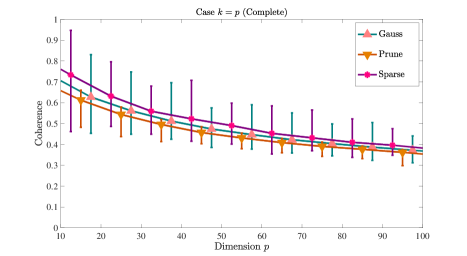
where $\left\|d_{i}\right\|_{2}=1$ for all $i\in[k]$ (see, e.g., Anandkumar et al., 2015). This coherence $\sigma(D)$ takes values in $[0,1]$ and is the cosine of the angle between two mixing component with the smallest mutual angle. It is intuitively clear that it is more difficult to recover latent mixing components with smaller angle between them. In practice, we set up the threshold $\overline{\sigma}$ to the mean value of the coherence for a given pair $(p,k)$ over large number of resampling (say $10,000$).

In the latter (sparse) case, we first sample a matrix from the normal distribution as described above and then zero-out half of the elements of this matrix. To construct the support, we sample another matrix from the normal distribution and zero-out all the elements exceeding the median value. If the obtained matrix has at least one column of all zeros or the respective atoms $d_{i}d_{i}^{\top}$ are not linearly independent, we resample such matrix.

Figure 5: Coherence of mixing matrices sampled with the sampling procedures described in Appendix D.1.1 in the complete (Left) and overcomplete (Right) cases. The lines correspond to median values over $1.000$ samples and the ticks, respectively, to the minimum and maximum values.

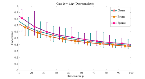Importantly, the obtained matrices in these three cases are not that much different for the purposes of the overcomplete recovery. Indeed, we can see from the a simple simulation experiment that they always have high coherences (see Figure 5). The coherence is especially high for lower dimensions $p$, such as 10 or 20, which are more amenable to experimental comparison. Therefore, one has to be careful when interpreting the results in such cases.

As we have seen in extensive experimental comparison, the OverICA algorithm recovers equally well mixing matrices sampled from any of these three sampling type.

D.1.2 The Population Case

This synthetic data simulate the infinite sample scenario. The algorithms are then provided with the exact subspace and one can measure how well the algorithms estimate the subspace in this noiseless setting. This type of synthetic data can only be used either with FOOBI or OverICA algorithms.

This data is for the scenario where the dimension $p$ of observations is fixed and the latent dimension $k$ is changing from $p$ up to $p(p+1)/2$. In particular, we sample $N_{rep}$ instances of synthetic data for different pairs of $(p,k)$:

1. Fix the dimension of observations $p$;

2. Repeat $N_{rep}=5$ times for different values of $k$:

   • Given a pair $(p,k)$, sample a mixing matrix $D$ (see Appendix D.1.1);

   • Construct the matrix $A:=D\odot D$;

   • Construct the matrix $C:=AA^{\top}$;

   • Extract an orthonormal basis $H:=\left[h_{i},i\in[k]\right]$ of the column space of the matrix $A$ from the matrix $C$ (in practice, as the largest $k$ eigenvectors or singular vectors of $C$);

   • Use the matrices $\left\{H_{1},\dots,H_{k}\right\}$ where each $H_{i}:=\mathrm{mat}(h_{i})$ for all $i\in[k]$, as a basis of the subspace as an input to the second step of the OverICA or FOOBI algorithms.

D.1.3 The Finite Sample Case: Fixed Dimensions

In this scenario, a finite sample $X:=\left\{x^{(1)},\dots,x^{(n)}\right\}$ is sampled exactly from the ICA model (1). This imitates presence of the finite sample noise but absence of the model misspecification. The amount of noise can be controlled by the number of samples $n$. This data can be used as an input to any overcomplete ICA algorithm.

In particular, we fix both dimensions $p$ and $k$ and vary the number of samples $n$:

1. Fix the dimension of the observations $p$ and the latent dimension $k$;

2. Repeat ($n_{rep}=10$ times) for different sample sizes $n$:

   • Sample a mixing matrix $D$ (see Appendix D.1.1);

   • Sample $n$ observations from the ICA model (1) with the uniformly distributed on the interval $[-0.5;0.5]$ sources.

   • Use this sample $X:=\left\{x^{(1)},\dots,x^{(n)}\right\}$ as an input.

This procedure results in $n_{rep}$ datasets for any $n$ for any pair of $(p,k)$.

D.1.4 The Finite Sample Case: Fixed Sample Size

This sampling procedure is almost identical to the one described in Section D.1.3 with the only difference that the sample size $n$ is fixed instead and the latent dimension $k$ is varied:

1. Fix the dimension of the observations $p$ and the sample size $n$;

2. Repeat ($N_{rep}=10$ times) for different latent dimensions $k$:

   • Sample a mixing matrix $D$ (see Appendix D.1.1);

   • Sample $n$ observations from the ICA model (1) with the uniformly distributed on the interval $[-0.5;0.5]$ sources.

   • Use this sample $X:=\left\{x^{(1)},\dots,x^{(n)}\right\}$ as an input.

It does not make sense to consider values of $k$ greater than $p(p+1)/2$, since in that case the matrix $A:=D\odot D$ does not have full column rank. In practice, we point out some interesting values of $k$: (a) $k=p$, (b) $k=p^{2}/4$ (corresponds to phase transition of OverICA), (c) $k=p(p-1)/2$ and $k=p(p+1)/2$. We mark these values with vertical green lines on plots for all experiments which use this sampling procedure.

D.2 Error Metrics

Given a ground truth mixing matrix $D$ and its estimate $\widehat{D}$, we introduce the following error metrics to measure the estimation quality. Note that for the computation of these error metrics we assume that every mixing component, i.e. every column of the mixing matrix, have unit norm in accordance with Assumption 2.1.

D.2.1 F-Error

We define the f-error, i.e. the Frobenius error, as:

$$\mathrm{err}_{F}(D,\widehat{D}):=\mathop{\rm min}\limits_{\sigma\in\mathcal{P}}\frac{\left\|D-\widehat{D}_{\sigma}\right\|_{F}^{2}}{\left\|D\right\|_{F}^{2}},$$

where $\left\|\cdot\right\|_{F}$ stands for the Frobenius norm of a matrix and we minimize the error over all possible permutations $\sigma\in\mathcal{P}$ of the columns of $\widehat{D}$ (with the Hungarian algorithm in practice (Kuhn, 1955)). Smaller values of this error are better.

D.2.2 A-Error

We define the a-error, i.e. the angle error, as:

$$\mathrm{err}_{C}(D,\widehat{D}) :=\frac{2}{k\pi}\;\mathop{\rm min}\limits_{\sigma\in\mathcal{P}}\;\left[\sum_{i\in[k]}\mathrm{acos}\left(\gamma\right)\right],$$

$$\gamma :=\frac{\left|\langle d_{i},\widehat{d}_{\sigma(i)}\rangle\right|}{\left\|d_{i}\right\|_{2}\left\|\widehat{d}_{\sigma(i)}\right\|_{2}},$$

where $\left\|\cdot\right\|_{2}$ stands for the Euclidean norm of a vector, the $d_{i}$ or $\widehat{d}_{i}$ are the $i$-th columns of the matrices $D$ or $\widehat{D}$, respectively, and we again minimize the error over all possible permutations of the columns of $\widehat{D}$. Note that $\pi\approx 3.14$. The a-error takes values in the interval $[0,1]$ and smaller values of the a-error are better. Note the relation of the a-error to the coherence measure (27).

D.2.3 Number of Recovered Atoms

Since neither a- nor f-errors measure the quality of recovery of individual mixing components, we also introduce another metric for the estimation recovery, which measures the number of “perfectly” recovered components.

Perfect Recovery.

By a “perfectly” recovered component we mean a component $\widehat{d}_{\sigma(i)}$ which is at most angle $\theta$ far from its respective ground truth value $d_{i}$, i.e.

$$\mathrm{acos}\left(\gamma\right)=\mathrm{acos}\left(\frac{\left|\langle d_{i},\widehat{d}_{\sigma(i)}\rangle\right|}{\left\|d_{i}\right\|_{2}\left\|\widehat{d}_{\sigma(i)}\right\|_{2}}\right)\leq\theta,$$

where $\sigma$ corresponds to the optimal permutation in terms of a-error as described above.

Normalized Recovery Vector.

We define the normalized recovery vector $r\in[0,1]^{k}$ such that its $i$-th component is equal to the fraction of at least $i$ “perfectly” recovered (in terms of the parameter $\theta$) components over $N_{rep}$ repetitions of an experiment. For example, if $k=5$ and $N_{rep}=3$ and an algorithm recovers “perfectly” 2, 4, and 3 components in these 3 runs, then the normalized recovery vector is $r=(1,1,2/3,1/3,0)$. In the plots in Section 3, we use black for 100% recovery of at least $i\leq k$ components, i.e. 1’s, and white for never recovering $i\leq k$ components or more “perfectly,” i.e. 0’s. The intermediate values are shown in grey. We consider the threshold value of $\theta:=\mathrm{acos}(0.99)$, which corresponds to the angle $\phi:=\theta*180/\pi\approx 8$.

Figure 6: Comparison in the finite sample regime – additional plots. See explanation in Section 3.2.

Figure 7: Additional plots for the runtime comparison experiment from Section 3.3.

D.3 Computational and Memory Complexities

In Table 1, we summarize the computational and memory complexities of the FOOBI algorithm (De Lathauwer et al., 2007), the Fourier PCA algorithm (Goyal et al., 2014), our OverICA algorithm and its modification which replaces the first step and two different implementations, GenCov from Section 2.3 and CUM from Appendix B.2, of the first step of our algorithm.

Complexity of Generalized Covariances.

Constructing $s$ generalized covariances, where usually $s=O(k)$, requires $O(p^{2}s)$ memory and $O(nsp^{2})$ time complexities. Extracting further $k$ largest singular vectors would require additional $O(k^{2}p^{2})$ time, but the other term is dominant since $s=O(k)$ and $n$ is larger than $k$.

Complexity of the Fourth-Order Cumulant.

A flattening $C$ of the fourth-order cumulant (as described in Appendix B.2) would require $O(p^{4})$ memory space and it can be constructed in $O(np^{4})$ time. The algorithms further compute it’s $k$ largest singular vectors, which requires $O(k^{2}p^{2})$ time.

Complexity of FOOBI.

The first step of FOOBI is based on the construction of the flattening of the fourth-order cumulant and therefore requires the complexities presented above. The second step is more involved and requires construction of $O(k^{4})$ and $O(p^{4}k^{2})$ matrices and computation of the eigen decomposition of a $O(k^{4})$ matrix. This leads to additional $O(p^{4}k^{2}+k^{4})$ memory and at least $O(k^{6})$ computational complexity requirements. It further solves orthogonal joint matrix diagonalization (Bunse-Gerstner et al., 1993; Cardoso and Souloumiac, 1993, 1996) which requires at least $O(k^{4})$ runtime per sweep.

Complexity of Fourier PCA.

The complexity of Fourier PCA is dominated by the first step where two fourth-order generalized cumulants are constructed. This requires $O(p^{4})$ memory and $O(np^{4})$ time complexities, although we notice in practice that the constant hidden in $O(\cdot)$ for the time is rather large.

Complexity of OverICA.

Since one iteration of FISTA (see Algorithm 2) requires $O(p^{3})$ and the number of iterations is not high, the algorithm is dominated by the first step. Then it takes the respective time of the construction of generalized covariance or the fourth-order cumulant and then computation of the SVD.

We design the following synthetic experiment to compare the runtime. We sample finite sample synthetic data as described in Appendix D.1.4 with the fixed sample size $n=100,000$ and observed dimension $p=20$. The latent dimension takes values between $k=p=20$ and $k=p^{2}/4=100$ in steps of $20$. We measure runtimes in seconds and display the results in log-linear scale. This comparison is for illustrative purposes only since the runtime depends on different factors. In particular, our Matlab/C++ code for FOOBI is highly optimized for runtime performance, while our Matlab implementations of OverICA and Fourier PCA are less so. The parameter $s$ for OverICA is set to $s=10k$. We show a head-to-head comparison of runtime in Figure 7. We observe that f- and a-errors of OverICA and FOOBI are nearly the same which is in accord with the experimental results from Section 3.2.

D.4 Additional Experiments

In this section, we present some more plots for the finite sample experiment from Section 3.2 (see Figure 6) and for the runtime experiment from Section 3.3 (see Figure 7).

References

- Anandkumar et al. (2015) A. Anandkumar, R. Ge, and M. Janzamin. Learning overcomplete latent variable models through tensor methods. In Proceedings of the Conference on Learning Theory (COLT), 2015.
- Arora et al. (2012) S. Arora, R. Ge, A. Moitra, and S. Sachdeva. Provable ICA with unknown Gaussian noise, with implications for Gaussian mixtures and autoencoders. In Advances in Neural Information Processing Systems (NIPS), 2012.
- Beck and Teboulle (2009) A. Beck and M. Teboulle. A fast iterative shrinkage-thresholding algorithm for linear inverse problems. SIAM Journal on Imaging Sciences, 2(1):183–202, 2009.
- Bengio et al. (2013) Y. Bengio, A. Courville, and P. Vincent. Representation learning: A review and new perspectives. IEEE Transactions on Pattern Analysis and Machine Intelligence, 35(8):1798–1828, 2013.
- Bhardwaj et al. (2015) A. Bhardwaj, P. Rostalski, and R. Sanyal. Deciding polyhedrality of spectrahedra. SIAM Journal on Optimization, 25(3):1873–1884, 2015.
- Bhaskara et al. (2014a) A. Bhaskara, M. Charikar, A. Moitra, and A. Vijayaraghavan. Smoothed analysis of tensor decompositions. In Proceedings of the Annual ACM Symposium on Theory of Computing (STOC), 2014a.
- Bhaskara et al. (2014b) A. Bhaskara, M. Charikar, and A. Vijayaraghavan. Uniqueness of tensor decompositions with applications to polynomial idenfifiability. In Proceedings of the Conference on Learning Theorey (COLT), 2014b.
- Bovier (2005) A. Bovier. Extreme Values of Random Processes. Lecture Notes Technische Universität Berlin, 2005.
- Bunse-Gerstner et al. (1993) A. Bunse-Gerstner, R. Byers, and V. Mehrmann. Numerical methods for simultaneous diagonalization. SIAM Journal on Matrix Analysis and Applications, 14(4):927–949, 1993.
- Cardoso and Souloumiac (1993) J.-F. Cardoso and A. Souloumiac. Blind beamforming for non-Gaussian signals. In IEE Proceedings F - Radar and Signal Processing. IEEE, 1993.
- Cardoso and Souloumiac (1996) J.-F. Cardoso and A. Souloumiac. Jacobi angles for simultaneous diagonalization. SIAM Journal on Matrix Analysis and Applications, 17(1):161–164, 1996.
- Chen and Donoho (1994) S.S. Chen and D.L. Donoho. Basis Pursuit. Technical report, Stanford University, 1994.
- Chen et al. (1998) S.S. Chen, D.L. Donoho, and M.A. Saunders. Atomic decomposition by basis pursuit. SIAM Journal on Scientific Computing, 20(1):33–61, 1998.
- Coates et al. (2011) A. Coates, H. Lee, and A.Y. Ng. An analysis of single-layer networks in unsupervised feature learning. In Proceedings of the International Conference on Artificial Intelligence and Statistics (AISTATS), 2011.
- Comon (1994) P. Comon. Independent component analysis, A new concept? Signal Processing, 36(3):287–314, 1994.
- Comon and Jutten (2010) P. Comon and C. Jutten. Handbook of Blind Sourse Separation: Independent Component Analysis and Applications. Academic Press, 2010.
- Comon and Rajih (2006) P. Comon and M. Rajih. Blind identification of under-determined mixtures based on the characteristic function. Signal Processing, 86(9):2271–2281, 2006.
- Daubechies (1988) I. Daubechies. Time-frequency localization operators: A geometric phase space approach. IEEE Transactions on Information Theory, 34(4):604–612, 1988.
- De Lathauwer et al. (2007) L. De Lathauwer, J. Castaing, and J.-F. Cardoso. Fourth-order cumulant-based blind identification of underdetermined mixtures. IEEE Transactions on Signal Processing, 55(6):2965–2973, 2007.
- Duchi et al. (2008) J. Duchi, S. Shalev-Shwartz, Y. Singer, and T. Chandra. Efficient projections onto the -ball for learning in high dimensions. In Proceedings of the International Conference on Machine Learning (ICML), 2008.
- Goyal et al. (2014) N. Goyal, S. Vempala, and Y. Xiao. Fourier PCA and robust tensor decomposition. In Proceedings of the Annual ACM Symposium on Theory of Computing (STOC), 2014.
- Grant et al. (2006) M. Grant, S. Boyd, and Y. Ye. Disciplined convex programming. In Global Optimization: from Theory to Implementation, Nonconvex Optimization and Its Applications. Springer, 2006.
- Hunter and Lange (2004) D.R. Hunter and K. Lange. A tutorial on MM algorithms. The American Statistician, 58(1):30–37, 2004.
- Hyvärinen (1999) A. Hyvärinen. Fast and robust fixed-point algorithms for independent component analysis. IEEE Transactions on Neural Networks, 10(3):626–634, 1999.
- Hyvärinen (2005) A. Hyvärinen. Estimation of non-normalized statistical models by score matching. Journal of Machine Learning Research (JMLR), 6:695–708, 2005.
- Hyvärinen et al. (2001) A. Hyvärinen, J. Karhunen, and E. Oja. Independent Component Analysis. Wiley, 2001.
- Krizhevsky et al. (2014) A. Krizhevsky, V. Nair, and G. Hinton. The CIFAR-10 dataset. University of Toronto, 2014. URL http://www.cs.toronto.edu/kriz/cifar.html.
- Kuhn (1955) H.W. Kuhn. The Hungarian method for the assignment problem. Naval Research Logistics Quarterly, 2(1-2):83–97, 1955.
- Le et al. (2011) Q.L. Le, A. Karpenko, J. Ngiam, and A.Y. Ng. ICA with reconstruction cost for efficient overcomplete feature learning. In Advances in Neural Information Processing Systems (NIPS), 2011.
- Lewicki and Sejnowski (2000) M.S. Lewicki and T.J Sejnowski. Learning overcomplete representations. Neural Computation, 12(2):337–365, 2000.
- Ma et al. (2016) T. Ma, J. Shi, and D. Steurer. Polynomial-time tensor decompositions with sum-of-squares. In Annual Symposium on Foundations of Computer Science (FOCS), 2016.
- Olshausen and Field (1996) B.A. Olshausen and D.J. Field. Emergence of simple-cell receptive field properties by learning a sparse code for natural images. Nature, 381:607–609, 1996.
- Olshausen and Field (1997) B.A. Olshausen and D.J. Field. Sparse coding with an overcomplete basis set: A strategy employed by V1? Vision Research, 37(23):3311–3325, 1997.
- Podosinnikova et al. (2016) A. Podosinnikova, F. Bach, and S. Lacoste-Julien. Beyond CCA: Moment matching for multi-view models. In Proceedings of the International Conference on Machine Learning (ICML), 2016.
- Saunderson (2011) J. Saunderson. Subspace identification via convex optimization. PhD thesis, Massachusetts Institute of Technology, 2011.
- Saunderson et al. (2012) J. Saunderson, V. Chandrasekaran, P.A. Parrilo, and A.S. Willsky. Diagonal and low-rank matrix decompositions, correlation matrices, and ellipsoid fitting. Technical report, arXiv:1204.1220v1, 2012.
- Saunderson et al. (2013) J. Saunderson, P.A. Parrilo, and A.S. Willsky. Diagonal and low-rank decompositions and fitting ellipsoids to random points. In Proceedings of the IEEE Conference on Decision and Control (CDC), 2013.
- Sokol et al. (2014) A. Sokol, M.H. Maathuis, and B. Falkeborg. Quantifying identifiability in independent component analysis. Electronic Journal of Statistics, 8:1438–1459, 2014.
- Sturm (1999) J.F. Sturm. Using SeDuMi 1.02, A MATLAB toolbox for optimization over symmetric cones. Optimization Methods and Software, 11(12):625–633, 1999.
- Teh et al. (2003) Y.W. Teh, M. Welling, S. Osindero, and G.E. Hinton. Energy-based models for sparse overcomplete representations. Journal of Machine Learning Research (JMLR), 4:1235–1260, 2003.
- Yeredor (2000) A. Yeredor. Blind source separation via the second characteristic function. Signal Processing, 80(5):897–902, 2000.