Sequential Skip Prediction with Few-shot
in Streamed Music Contents

Abstract.

This paper provides an outline of the algorithms submitted for the WSDM Cup 2019 Spotify Sequential Skip Prediction Challenge (team name: mimbres). In the challenge, complete information including acoustic features and user interaction logs for the first half of a listening session is provided. Our goal is to predict whether the individual tracks in the second half of the session will be skipped or not, only given acoustic features. We proposed two different kinds of algorithms that were based on metric learning and sequence learning. The experimental results showed that the sequence learning approach performed significantly better than the metric learning approach. Moreover, we conducted additional experiments to find that significant performance gain can be achieved using complete user log information.

1. Introduction

In online music streaming services such as Spotify, a huge number of active users are interacting with a library of over 40 million audio tracks. Here, an important challenge is to recommend the right music item to each user. To this end, there has been a large related body of works in music recommender systems. A standard approach was to construct a global model based on user’s play counts(Celma, 2010; Van den Oord et al., 2013) and acoustic features(Van den Oord et al., 2013). However, a significant aspect missing in these works is how a particular user sequentially interacts with the streamed contents. This can be thought as a problem of personalization(Cho et al., 2002) with few-shot, or meta-learning(Mishra et al., 2018) with external memory(Santoro et al., 2016). The WSDM Cup 2019 tackles this issue by defining a new task with a real dataset(Brost et al., 2019). We can summarize the task as follows:

• The length $L^{i}$ of an $i$-th listening session for a blinded-particular user varies in the range from 10 to 20. We omit $i$ for readability from next page.

• We denote the input sequence (Figure 1) from the first half (=support) and second half(=query) of each session $i$ as $X^{i}_{s}$ and $X^{i}_{q}$, respectively.

• $X^{i}_{s}$ contains complete information including session logs and acoustic features.

• $X^{i}_{q}$ contains only acoustic features.

• $Y^{i}_{s}$ is the labels representing whether the supports were skipped$(=1)$ or not$(=0)$.

• Given a set of inputs $\{X^{i}_{s},Y^{i}_{s},X^{i}_{q}\}$, our task is to predict $Y^{i}_{q}$ (Figure 2).

One limitation of our research was that we did not make use of any external dataset nor pre-trained model from them. The code and evaluation results are available online.

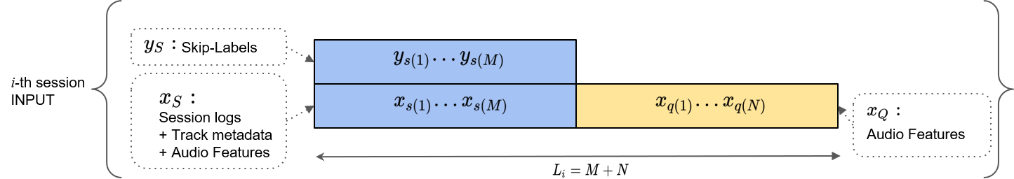
Several flies, spanning two columns of text

Figure 1. Input structure; The blue and yellow blocks represent the inputs of supports and queries for prediction, respectively.

2. Model Architectures

A fly image, to $1^{\prime\prime}\times 1^{\prime\prime}$

Figure 2. Output structure; The red block represents the skip-labels to be predicted for the $i$-th session.

In this section, we explain two different branches of algorithms based on 1) metric learning, and 2) sequence learning. In metric learning-based approach, one key feature is that we do not assume the presence of orders in a sequence. This allows us to formulate the skip prediction problem in a similar way with the previous works(Sung et al., 2018) on few-shot learning that learns to compare.

In sequence learning-based approach, we employ temporal convolution layers that can learn or memorize information by assuming the presence of orders in a sequence. In this fashion, we formulate the skip prediction problem as a meta-learning(Mishra et al., 2018) that learns to refer past experience.

2.1. Metric Learning

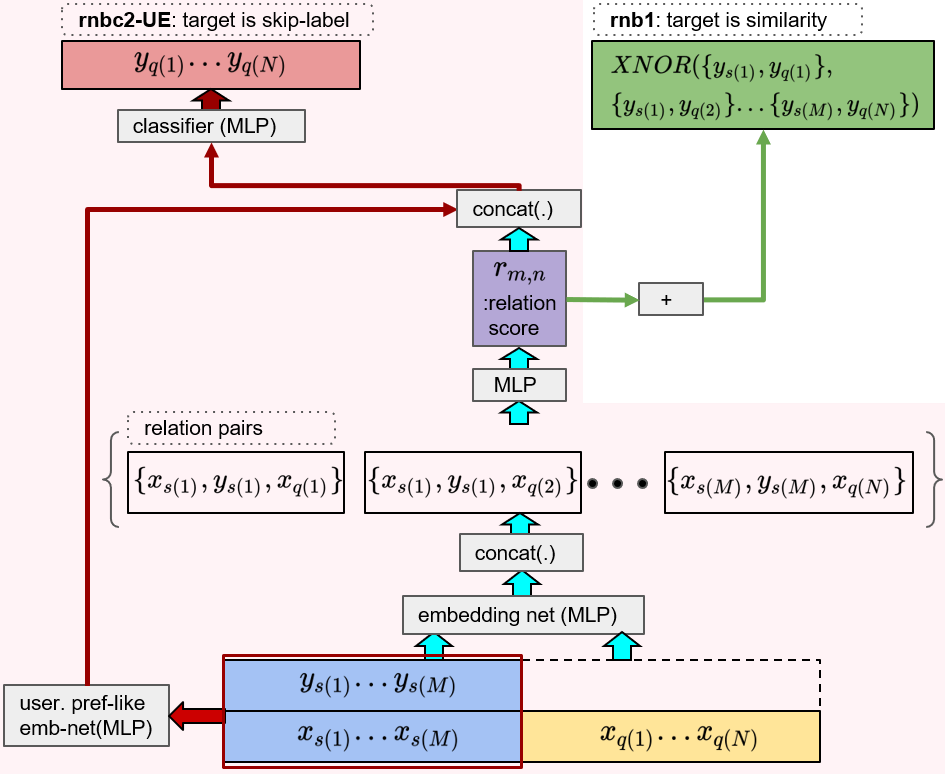
Figure 3. “rnb1” is a relation network-based few-shot metric learner. It can predict a pair-wise similarity (green arrows) by learnt latent metric space: it constructs all possible relation pairs from the few-shot features and labels. “rnbc2-UE” (pink) shares the structure of “rnb1”, and it can be trained as a few-shot classifier that directly predicts skip-labels.

This model aims to learn how to compare a pair of input acoustic features, through a latent metric space, within the context given from the supports. Previously, Sung et al.(Sung et al., 2018) proposed a metric learning for few-shot classification. The relation score $r_{m,n}$ for a pair of support and query inputs, $\{x_{s(m)},x_{q(n)}\}$ and the label $y_{s(m)}$ can be defined by:

(1) $$r_{m,n}=\text{RN}(~{}C(~{}f_{\theta}(x_{s(m)},f_{\theta}(x_{q(n)}),y_{s(m)}~{})~{}),$$

where RN$(.)$ is the relation networks(Santoro et al., 2017), $f_{\theta}$ is an MLP for embedding network, and $C(.)$ is a concatenation operator. In the original model(Sung et al., 2018) denoted by rnb1, the sum of the relation score is trained to match the binary target similarity. The target similarity can be computed with XNOR operation for each relation pair. For example, a pair of items that has same labels will have a target similarity $1$; otherwise $0$. The final model is denoted as rnbc2-UE (Figure 3) with:

1. training the classifier to predict the skip-labels directly, instead of similarity.

2. trainable parameters to calculate weighted sum of the relation score $r$,

3. additional embedding layers (the red arrows in Figure 3) to capture the user preference-like.

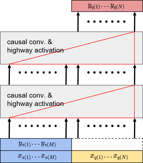
Figure 4. “seq1HL” has 2-stack of causal encoders. A red right triangle represents causal encoder, that is not allowed to observe future inputs.

2.2. Sequence Learning

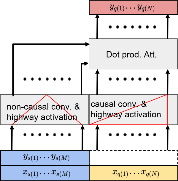
Figure 5. “att(seq1eH(S), seq1eH(Q))” has non-causal encoder for the supports. This allows model to observe future inputs, as represented with a red isosceles triangle.

In Figure 4, this model consists of dilated convolution layers followed by highway(Srivastava et al., 2015)-activations or GLUs (gated linear units(Dauphin et al., 2016)). A similar architecture can be found in the text encoder part of a recent TTS (Text-to-speech) system(Tachibana et al., 2018). In practice, we found that non-auto-regressive (non-AR)-models performed consistently better than the AR-models. This was explainable as the noisy outputs of the previous steps degraded the outputs of the next steps cumulatively. The final model, seq1HL, has the following features:

1. a non-AR model,

2. highway-activations with instance norm(Vedaldi, 2016), instead of using GLUs,

3. $1$-$d$ causal convolution layers with a set of dilation parameters $d=\{1,2,4,8,16\}$ and kernel size $k=2$,

4. in train, parameters are updated using the loss of $Y_{q}$, instead of the entire loss of $\{Y_{q},Y_{q}\}$.

We have two variants of the sequence learning model with attention modules. The model in Figure 5 has separate encoders for supports and queries. The support encoder has $1$-stack of non-causal convolution with a set of dilation parameters $d=\{1,3,9\}$ and kernel size $k=3$. The query encoder has $1$-stack of causal convolution with a set of dilation parameters $d=\{1,2,4\}$ and kernel size $k=\{2,2,3\}$. These encoders are followed by a dot product attention operation(Vaswani et al., 2017).

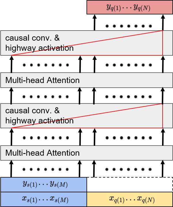
Figure 6. SNAIL(Mishra et al., 2018)-like model. We removed the first embedding layer, and trained it as a non-AR model.

In contrast with the models mentioned above, SNAIL(Mishra et al., 2018) (in Figure 6) has attention module at the bottom, and the causal convolution layer follows. For the multi-head attention, we set the number of head to 8.

3. Experiments

3.1. Pre-processing

From the Spotify dataset(Brost et al., 2019), we decoded the categorical text labels in session logs into one-hot vectors. Other integer values from the logs, such as “number of times the user did a seek forward within track” were min-max normalized after taking logarithm. We didn’t make use of dates. The acoustic features were standardized to have mean=$0$ with std=$1$.

3.2. Evaluation Metric

The primary metric for the challenge was Mean Average Accuracy (MAA), with the average accuracy defined by $AA=\sum_{i=1}^{T}A(i)L(i)/{T},$ where $T$ is the number of tracks to be predicted for the given session, $A(i)$ is the accuracy at position $i$ of the sequence, and $L(i)$ is the boolean indicator for if the $i$-th prediction was correct.

3.3. Training

In all experiments displayed in Table 1, we trained the models using $80$% of train set. The rest of train set was used for validation. rnb1 and rnb2-UE was trained with MSE loss. All other models were trained with binary cross entropy loss. We used Adam(Kingma and Ba, 2014) optimizer with learning rate $10^{-3}$, annealed by 30% for every 99,965,071 sessions (= 1 epoch). Every training was stopped within 10 epochs, and the training hour varied from 20 to 48. We uniformly applied the batch-size 2,048. For the baseline algorithms that have not been submitted, we display the validation MAA instead. The total size of trainable parameters for each model can vary. For comparison of model architectures, we maintained the in-/output dimensions of every repeated linear units in metric learning as 256. In sequence learning, we maintained the size of in-/output channels as 256 for every encoder units.

Table 1. Main Results

Model	Category	MAA(ofc)	MAA(val)
rnb1	M	-	0.540
rnb2-UE	M	-	0.564
rnbc2-UE	M	0.574	0.574
seq1eH (1-stack)	S	0.633	0.633
seq1HL (2-stack)	S	0.637	0.638
att(seq1eH(S), seq1eH(Q))	S	-	0.633
self-att. transformer	S	-	0.631
replicated-SNAIL	S	-	0.630

• MAA(ofc) from official evaluation; MAA(val) from our validation; M and S denote metric and sequence learning, respectively; rnb1 was the replication of “learning to compare”(Sung et al., 2018); rnbc2-UE and seq1HL were our final model for metric and sequence learning, respectively;

3.4. Main Results and Discussion

Note that we only discuss here the results from non-AR setting. The main results are displayed in Table 1. We can compare the metric learning-based algorithms in the first three rows. rnb1 was the firstly implemented algorithm. rnb2-UE had two additional embedding layers. It achieved 2.4%p improvements over rnb1. The final model, rnbc2-UE additionally achieved 1%p improvements by changing the target label from similarity to skip-labels.

The five rows from the bottom display the performance of sequence learning-based algorithms. seq1eH and seq1HL shared the same architecture, but differed in the depth of the networks. seq1HL achieved the best result, and it showed 0.5%p improvement over seq1eH. att(seq1eH(S), seq1eH(Q)) showed a comparable performance with seq1eH. The trans-former(Vaswani et al., 2017) and SNAIL(Mishra et al., 2018) were also attention-based models. However, we could observe that sequence learning-based model without attention unit worked better.

Overall, the sequence learning-based approaches outperformed the metric learning-based approaches by at least 5.9%p. The large difference in performance implied that sequence learning was more efficient, and the metric learning-based models were missing crucial information from the sequence data.

3.5. How helpful would it be if complete information was provided to query sets?

Table 2. The effect of complete information provided to query

Model	User-logs	Acoustic feat.	Skip-label	MAA(val)
Teacher	use	use	-	0.849
seq1HL	-	use	-	0.638

So far, the input query set $X_{q}$ has been defined as acoustic features (see Figure 1). In this experiment, we trained a new model Teacher using both user-logs and acoustic features that were available in dataset. In Table 2, the performance of the Teacher was 21.1%p higher than our best model seq1HL. This revealed that the user-logs for $X_{q}$ might contain very useful information for sequential skip prediction. In future work, we will discover how to distill the knowledge.

4. Conclusions

In this paper, we have described two different approaches to solve the sequential skip prediction task with few-shot in online music service. The first approach was based on metric learning, which aimed to learn how to compare the music contents represented by a set of acoustic features and user interaction logs. The second approach was based on sequence learning, which has been widely used for capturing temporal information or learning how to refer past experience. In experiments, our models were evaluated in WSDM Cup 2019, using the real dataset provided by Spotify. The main results revealed that the sequence learning approach worked consistently better than metric learning. In the additional experiment, we verified that giving a complete information to the query set could improve the prediction accuracy. In future work, we will discover how to generate or distill these knowledge by the model itself.

- (1)
- Brost et al. (2019) Brian Brost, Rishabh Mehrotra, and Tristan Jehan. 2019. The Music Streaming Sessions Dataset. In Proc. the 2019 Web Conference. ACM.
- Celma (2010) Oscar Celma. 2010. Music recommendation. In Music recommendation and discovery. Springer, 43–85.
- Cho et al. (2002) Yoon Ho Cho, Jae Kyeong Kim, and Soung Hie Kim. 2002. A personalized recommender system based on web usage mining and decision tree induction. Expert systems with Applications 23, 3 (2002), 329–342.
- Dauphin et al. (2016) Yann N Dauphin, Angela Fan, Michael Auli, and David Grangier. 2016. Language modeling with gated convolutional networks. arXiv preprint arXiv:1612.08083 (2016).
- Kingma and Ba (2014) Diederik P Kingma and Jimmy Ba. 2014. Adam: A method for stochastic optimization. arXiv preprint arXiv:1412.6980 (2014).
- Mishra et al. (2018) Nikhil Mishra, Mostafa Rohaninejad, Xi Chen, and Pieter Abbeel. 2018. A simple neural attentive meta-learner. In Proc. ICLR 2018.
- Santoro et al. (2016) Adam Santoro, Sergey Bartunov, Matthew Botvinick, Daan Wierstra, and Timothy Lillicrap. 2016. Meta-learning with memory-augmented neural networks. In Proc. ICML 2016. 1842–1850.
- Santoro et al. (2017) Adam Santoro, David Raposo, David G Barrett, Mateusz Malinowski, Razvan Pascanu, Peter Battaglia, and Timothy Lillicrap. 2017. A simple neural network module for relational reasoning. In Proc. NIPS 2017. 4967–4976.
- Srivastava et al. (2015) Rupesh Kumar Srivastava, Klaus Greff, and Jürgen Schmidhuber. 2015. Highway networks. arXiv preprint arXiv:1505.00387 (2015).
- Sung et al. (2018) Flood Sung, Yongxin Yang, Li Zhang, Tao Xiang, Philip HS Torr, and Timothy M Hospedales. 2018. Learning to compare: Relation network for few-shot learning. In Proc. CVPR 2018. 1199–1208.
- Tachibana et al. (2018) Hideyuki Tachibana, Katsuya Uenoyama, and Shunsuke Aihara. 2018. Efficiently trainable text-to-speech system based on deep convolutional networks with guided attention. In Proc. ICASSP 2018. IEEE, 4784–4788.
- Van den Oord et al. (2013) Aaron Van den Oord, Sander Dieleman, and Benjamin Schrauwen. 2013. Deep content-based music recommendation. In Proc. NIPS 2013. 2643–2651.
- Vaswani et al. (2017) Ashish Vaswani, Noam Shazeer, Niki Parmar, Jakob Uszkoreit, Llion Jones, Aidan N Gomez, Łukasz Kaiser, and Illia Polosukhin. 2017. Attention is all you need. In Proc. NIPS 2017. 5998–6008.
- Vedaldi (2016) Victor Lempitsky Dmitry Ulyanov Andrea Vedaldi. 2016. Instance Normalization: The Missing Ingredient for Fast Stylization. arXiv preprint arXiv:1607.08022 (2016).