DistCache: Provable Load Balancing for Large-Scale Storage Systems
with Distributed Caching

Abstract

Load balancing is critical for distributed storage to meet strict service-level objectives (SLOs). It has been shown that a fast cache can guarantee load balancing for a clustered storage system. However, when the system scales out to multiple clusters, the fast cache itself would become the bottleneck. Traditional mechanisms like cache partition and cache replication either result in load imbalance between cache nodes or have high overhead for cache coherence.

We present DistCache, a new distributed caching mechanism that provides provable load balancing for large-scale storage systems. DistCache co-designs cache allocation with cache topology and query routing. The key idea is to partition the hot objects with independent hash functions between cache nodes in different layers, and to adaptively route queries with the power-of-two-choices. We prove that DistCache enables the cache throughput to increase linearly with the number of cache nodes, by unifying techniques from expander graphs, network flows, and queuing theory. DistCache is a general solution that can be applied to many storage systems. We demonstrate the benefits of DistCache by providing the design, implementation, and evaluation of the use case for emerging switch-based caching.

1 Introduction

Modern planetary-scale Internet services (e.g., search, social networking and e-commerce) are powered by large-scale storage systems that span hundreds to thousands of servers across tens to hundreds of racks [1, 2, 3, 4]. To ensure satisfactory user experience, the storage systems are expected to meet strict service-level objectives (SLOs), regardless of the workload distribution. A key challenge for scaling out is to achieve load balancing. Because real-world workloads are usually highly-skewed [5, 6, 7, 8], some nodes receive more queries than others, causing hot spots and load imbalance. The system is bottlenecked by the overloaded nodes, resulting in low throughput and long tail latencies.

Caching is a common mechanism to achieve load balancing [9, 10, 11]. An attractive property of caching is that caching $O(n\log n)$ hottest objects is enough to balance $n$ storage nodes, regardless of the query distribution [9]. The cache size only relates to the number of storage nodes, despite the number of objects stored in the system. Such property leads to recent advancements like SwitchKV [10] and NetCache [11] for balancing clustered key-value stores.

Unfortunately, the small cache solution cannot scale out to multiple clusters. Using one cache node per cluster only provides intra-cluster load balancing, but not inter-cluster load balancing. For a large-scale storage system across many clusters, the load between clusters (where each cluster can be treated as one “big server”) would be imbalanced. Using another cache node, however, is not sufficient, because the caching mechanism requires the cache to process all queries to the $O(n\log n)$ hottest objects [9]. In other words, the cache throughput needs to be no smaller than the aggregate throughput of the storage nodes.

As such, it requires another caching layer with multiple cache nodes for inter-cluster load balancing. The challenge is on cache allocation. Naively replicating hot objects to all cache nodes incurs high overhead for cache coherence. On the other hand, simply partitioning hot objects between the cache nodes would cause the load to be imbalanced between the cache nodes. The system throughput would still be bottlenecked by one cache node under highly-skewed workloads. Thus, the key is to carefully partition and replicate hot objects, in order to avoid load imbalance between the cache nodes, and to reduce the overhead for cache coherence.

We present DistCache, a new distributed caching mechanism that provides provable load balancing for large-scale storage systems. DistCache enables a “one big cache” abstraction, i.e., an ensemble of fast cache nodes acts as a single ultra-fast cache. DistCache co-designs cache allocation with multi-layer cache topology and query routing. The key idea is to use independent hash functions to partition hot objects between the cache nodes in different layers, and to apply the power-of-two-choices [12] to adaptively route queries.

Using independent hash functions for cache partitioning ensures that if a cache node is overloaded in one layer, then the set of hot objects in this node would be distributed to multiple cache nodes in another layer with high probability. This intuition is backed up by a rigorous analysis that leverages expander graphs and network flows, i.e., we prove that there exists a solution to split queries between different layers so that no cache node would be overloaded in any layer. Further, since a hot object is only replicated in each layer once, it incurs minimal overhead for cache coherence.

Using the power-of-two-choices for query routing provides an efficient, distributed, online solution to split the queries between the layers. The queries are routed to the cache nodes in a distributed way based on cache loads, without central coordination and without knowing what is the optimal solution for query splitting upfront. We leverage queuing theory to show it is asymptotically optimal. The major difference between our problem and the balls-and-bins problem in the original power-of-two-choices algorithm [12] is that our problem hashes objects into cache nodes, and queries to the same object reuse the same hash functions to choose hash nodes, instead of using a new random source to sample two nodes for each query. We show that the power-of-two-choices makes a “life-or-death” improvement in our problem, instead of a “shaving off a log $n$” improvement.

DistCache is a general caching mechanism that can be applied to many storage systems, e.g., in-memory caching for SSD-based storage like SwitchKV [10] and switch-based caching for in-memory storage like NetCache [11]. We provide a concrete system design to scale out NetCache to demonstrate the power of DistCache. We design both the control and data planes to realize DistCache for the emerging switch-based caching. The controller is highly scalable as it is off the critical path. It is only responsible for computing the cache partitions and is not involved in handling queries. Each cache switch has a local agent that manages the hot objects of its own partition.

The data plane design exploits the capability of programmable switches, and makes innovative use of in-network telemetry beyond traditional network monitoring to realize application-level functionalities—disseminating the loads of cache switches by piggybacking in packet headers, in order to aid the power-of-two-choices. We apply a two-phase update protocol to ensure cache coherence.

In summary, we make the following contributions.

• We design and analyze DistCache, a new distributed caching mechanism that provides provable load balancing for large-scale storage systems (§3).

• We apply DistCache to a use case of emerging switch-based caching, and design a concrete system to scale out an in-memory storage rack to multiple racks (§4).

• We implement a prototype with Barefoot Tofino switches and commodity servers, and integrate it with Redis (§5). Experimental results show that DistCache scales out linearly with the number of racks, and the cache coherence protocol incurs minimal overhead (§6).

2 Background and Motivation

2.1 Small, Fast Cache for Load Balancing

As a building block of Internet applications, it is critical for storage systems to meet strict SLOs. Ideally, given the per-node throughput $T$, a storage system with $n$ nodes should guarantee a total throughput of $n\cdot T$. However, real-world workloads are usually high-skewed, making it challenging to guarantee performance [5, 6, 7, 8]. For example, a measurement study on the Memcached deployment shows that about 60-90% of queries go to the hottest 10% objects [5].

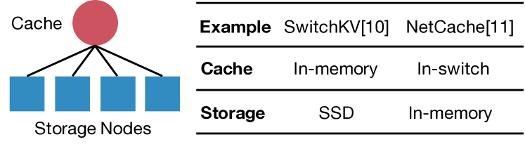
Figure 1: Background on caching. If the cache node can absorb all queries to the hottest $O(n\log n)$ objects, the load on the storage nodes is guaranteed to be balanced [9].

Caching is a common mechanism to achieve load balancing for distributed storage, as illustrated in Figure 1. Previous work has proven that if the cache node can absorb all queries to the hottest $O(n\log n)$ objects, then the load on $n$ storage servers is guaranteed to be balanced, despite query distribution and the total number of objects [9]. However, it also requires that the cache throughput needs to be at least $n\cdot T$ to not become the system bottleneck. Based on this theoretical foundation, SwitchKV [10] uses an in-memory cache to balance SSD-based storage nodes, and NetCache [11] uses a switch-based cache to balance in-memory storage nodes. Empirically, these systems have shown that caching a few thousand objects is enough for balancing a hundred storage nodes, even for highly-skewed workloads like Zipfian-0.9 and Zipfian-0.99 [10, 11].

2.2 Scaling out Distributed Storage

The requirement on the cache performance limits the system scale. Suppose the throughput of a cache node is $\widetilde{T}=c\cdot T$. The system can scale to at most a cluster of $c$ storage nodes. For example, given that the typical throughput of a switch is 10-100 times of that of a server, NetCache [11] can only guarantee load balancing for 10-100 storage servers. As such, existing solutions like SwitchKV [10] and NetCache [11] are constrained to one storage cluster, which is typically one or two racks of servers.

For a cloud-scale distributed storage system that spans many clusters, the load between the clusters can become imbalanced, as shown in Figure 2(a). Naively, we can put another cache node in front of all clusters to balance the load between clusters. At first glance, this seems a nice solution, since we can first use a cache node in each cluster for intra-cluster load balancing, and then use an upper-layer cache node for inter-cluster load balancing. However, now each cluster becomes a “big server”, of which the throughput is already $\widetilde{T}$. Using only one cache node cannot meet the cache throughput requirement, which is $m\widetilde{T}$ for $m$ clusters. While using multiple upper-layer cache nodes like Figure 2(b) can potentially meet this requirement, it brings the question of how to allocate hot objects to the upper-layer cache nodes. We examine two traditional cache allocation mechanisms.

Cache partition. A straightforward solution is to partition the object space between the upper-layer cache nodes. Each cache node only caches the hot objects of its own partition. In this case, a write query will update only one upper-layer cache node for cache coherence. Cache partition works well for uniform workloads, as the cache throughput can grow linearly with the number of cache nodes. But remember that under uniform workloads, the load on the storage nodes is already balanced, obviating the need for caching in the first place. The whole purpose of caching is to guarantee load balancing for skewed workloads. Unfortunately, cache partition strategy would cause load imbalance between the upper-layer cache nodes, because multiple hot objects can be partitioned to the same upper-layer cache node, making one cache node become the system bottleneck.

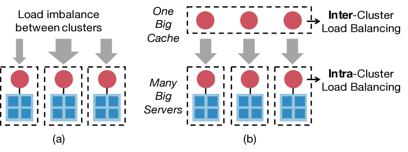
Figure 2: Motivation. (a) A cache node only guarantees load balancing for its own cluster, but the load between clusters can be unbalanced. (b) Use one cache node in each cluster for intra-cluster load balancing, and another layer of cache nodes for inter-cluster load balancing. The challenge is on cache allocation.

Cache replication. Cache replication replicates the hot objects to all the upper-layer cache nodes, and the queries can be uniformly sent to them. As such, cache replication ensures that the load between the cache nodes is balanced, and the throughput of caching can grow linearly with the number of cache nodes. However, cache replication introduces high overhead for cache coherence. When there is a write query to a cached object, the system needs to update both the primary copy at the storage node and the cached copies at the cache nodes, which often requires an expensive two-phase update protocol for cache coherence. As compared to cache partition which only caches a hot object in one upper-layer cache node, cache replication needs to update all the upper-layer cache nodes for cache coherence. This update procedure for cache coherence significantly degrades the throughput of write queries.

Challenge. Cache partition has low overhead for cache coherence, but cannot increase the cache throughput linearly with the number of cache nodes; cache replication achieves the opposite. Therefore, the main challenge is to carefully partition and replicate the hot objects, in order to $(i)$ avoid load imbalance between upper-layer cache nodes, and to $(ii)$ reduce the overhead for cache coherence.

3 DistCache Caching Mechanism Design

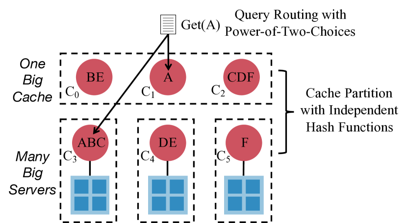
Figure 3: Key idea. $(i)$ Use independent hash functions to partition hot objects in different layers. $(ii)$ Use the power-of-two-choices to route queries, e.g., route $Get(A)$ to either cache node $C_{1}$ or cache node $C_{3}$ based on cache load.

3.1 Key Idea

We design DistCache, a new distributed caching mechanism to address the challenge described in §2.2. As illustrated by Figure 3, our key idea is to use independent hash functions for cache allocation and the power-of-two-choices for query routing, in order to balance the load between cache nodes. Our mechanism only caches an object at most once in a layer, incurring minimal overhead for cache coherence. We first describe the mechanism and the intuitions, and then show why it works in §3.2.

Cache allocation with independent hash functions. Our mechanism partitions the object space with independent hash functions in different layers. The lower-layer cache nodes primarily guarantee intra-cluster load balancing, each of which only caches hot objects for its own cluster, and thus each cluster appears as one “big server”. The upper-layer cache nodes are primarily for inter-cluster load balancing, and use a different hash function for partitioning. The intuition is that if one cache node in a layer is overloaded by receiving too many queries to its cached objects, because the hash functions of the two layers are independent, the set of hot objects would be distributed to multiple cache nodes in another layer with high probability. Figure 3 shows an example. While cache node $C_{3}$ in the lower layer is overloaded with three hot objects ($A$, $B$ and $C$), the three objects are distributed to three cache nodes ($C_{0}$, $C_{1}$ and $C_{2}$) in the upper layer. The upper-layer cache nodes only need to absorb queries for objects (e.g., $A$ and $B$) that cause the imbalance between the clusters, and do not need to process queries for objects (e.g., $D$ and $F$) that already spread out in the lower-layer cache nodes.

Query routing with the power-of-two-choices. The cache allocation strategy only tells that there exists a way to handle queries without overloading any cache nodes, but it does not tell how the queries should be split between the layers. Conceivably, we could use a controller to collect global measurement statistics to infer the query distribution. Then the controller can compute an optimal solution and enforce it at the senders. Such an approach has high system complexity, and the responsiveness to dynamic workloads depends on the agility of the control loop.

Our mechanism uses an efficient, distributed, online solution based on the power-of-two-choices [12] to route queries. Specifically, the sender of a query only needs to look at the loads of the cache nodes that cache the queried object, and sends the query to the less-loaded node. For example, the query $Get(A)$ in Figure 3 is routed to either $C_{1}$ or $C_{3}$ based on their loads. The key advantage of our solution is that: it is distributed, so that it does not require a centralized controller or any coordination between senders; it is online, so that it does not require a controller to measure the query distribution and compute the solution, and the senders do not need to know the solution upfront; it is efficient, so that its performance is close to the optimal solution computed by a controller with perfect global information (as shown in §3.2). Queries to hit a lower-layer cache node can either pass through an arbitrary upper-layer node, or totally bypass the upper-layer cache nodes, depending on the actual use case, which we describe in §3.4.

author=Alan, color=green]We clarify better idea regarding the cache size. Cache size and multi-layer hierarchical caching. Suppose there are $m$ clusters and each cluster has $l$ servers. First, we let each lower-layer cache node cache $O(l\log l)$ objects for its own cluster for intra-cluster load balancing, so that a total of $O(ml\log l)$ objects are cached in the lower layer and each cluster appears like one “big server”. Then for inter-cluster load balancing, the upper-layer cache nodes only need to cache a total of $O(m\log m)$ objects. This is different from a single ultra-fast cache at a front-end that handles all $ml$ servers directly. In that case, $O(ml\log(ml))$ objects need to be cached based on the result in [9]. However, in DistCache, we have an extra upper-layer (with the same total throughput as $ml$ servers) to “refine” the query distribution that goes to the lower-layer, which reduces the effective cache size in the lower layer to $O(ml\log l)$. Thus, this is not a contradiction with the result in [9]. While these $O(m\log m)$ inter-cluster hot objects also need to be cached in the lower layer to enable the power-of-two-choices, most of them are also hot inside the clusters and thus have already been contained in the $O(ml\log l)$ intra-cluster hot objects.

Our mechanism can be applied recursively for multi-layer hierarchical caching. Specifically, applying the mechanism to layer $i$ can balance the load for a set of “big servers” in layer $i$-$1$. Query routing uses the power-of-k-choices for k layers. Note that using more layers actually increases the total number of cache nodes, since each layer needs to provide a total throughput at least equal to that of all storage nodes. The benefit of doing so is on reducing the cache size. When the number of clusters is no more than a few hundred, a cache node has enough memory with two layers.

3.2 Analysis

Prior work [9] has shown that caching $O(n\log n)$ hottest objects in a single cache node can balance the load for $n$ storage nodes for any query distribution. In our work, we replace the single cache node with multiple cache nodes in two layers to support a larger scale. Therefore, based on our argument on the cache size in §3.1, we need to prove that the two-layer cache can absorb all queries to the hottest $O(m\log m)$ objects under any query distribution for all $m$ clusters. We first define a mathematical model to formalize this problem.

System model. There are $k$ hot objects $\{o_{0},o_{1},\dots,o_{k-1}\}$ with query distribution $P=\{p_{0},p_{1},\dots,p_{k-1}\}$, where $p_{i}$ denotes the fraction of queries for object $o_{i}$, and $\sum_{i=0}^{k-1}p_{i}=1$. The total query rate is $R$, and the query rate for object $o_{i}$ is $r_{i}=p_{i}\cdot R$. There are in total $2m$ cache nodes that are organized to two groups $A=\{a_{0},a_{1},...,a_{m-1}\}$ and $B=\{b_{0},b_{1},...,b_{m-1}\}$, which represent the upper and lower layers, respectively. The throughput of each cache node is $\widetilde{T}$.

The objects are mapped to the cache nodes with two independent hash functions $h_{0}(x)$ and $h_{1}(x)$. Object $o_{i}$ is cached in $a_{j_{0}}$ in group $A$ and $b_{j_{1}}$ in group $B$, where $j_{0}=h_{0}(i)$ and $j_{1}=h_{1}(i)$. A query to $o_{i}$ can be served by either $a_{j_{0}}$ or $b_{j_{1}}$.

Goal. Our goal is to evaluate the total query rate $R$ the cache nodes can support, in terms of $m$ and $\widetilde{T}$, regardless of query distribution $P$, as well as the relationship between $k$ and $m$. Ideally, we would like $R\approx\alpha m\widetilde{T}$ where $\alpha$ is a small constant (e.g., $1$), so that the operator can easily provision the cache nodes to meet the cache throughput requirement (i.e., no smaller than the total throughput of storage nodes).

If we can set $k$ to be $O(m\log m)$, it means that the cache nodes can absorb all queries to the hottest $O(m\log m)$ objects, despite query distribution. Combining this result with the cache size argument in §3.1, we can prove that the distributed caching mechanism can provide performance guarantees for large-scale storage systems across multiple clusters.

author=Alan, color=green]We clarify our problem can be a matching problem. A perfect matching problem in a bipartite graph. The key observation of our analysis is that the problem can be converted to finding a perfect matching in a bipartite graph. Intuitively, if a perfect matching exists, the requests to $k$ hot objects can be completely absorbed from the two layers of cache nodes. Specifically, we construct a bipartite graph $G=(U,V,E)$, where $U$ is the set of vertices on the left, $V$ is the set of vertices on the right, and $E$ is the set of edges. Let $U$ represent the set of objects, i.e., $U=\{o_{0},o_{1},...,o_{k-1}\}$. Let $V$ represent the set of cache nodes, i.e., $V=A\cup B=\{a_{0},a_{1},...,a_{m-1},b_{0},b_{1},...,b_{m-1}\}$. Let $E$ represent the hash functions mapping from the objects to the cache nodes, i.e., $E=\{e_{o_{i},a_{j_{0}}}|h_{0}(i)=j_{0}\}\cup\{e_{o_{i},b_{j_{1}}}|h_{1}(i)=j_{1}\}$. Given a query distribution $P$ and a total query rate $R$, we define a perfect matching in $G$ to represent that the workload can be supported by the cache nodes.

Definition 1.

Let $\Gamma(v)$ be the set of neighbors of vertex $v$ in $G$. A weight assignment $W=\{w_{i,j}\in[0,\widetilde{T}]|e_{i,j}\in E\}$ is a perfect matching of $G$ if

1. $\forall o_{i}\in U:\quad\sum_{v\in\Gamma(o_{i})}w_{o_{i},v}=p_{i}\cdot R$, and

2. $\forall v\in V:\quad\sum_{u\in\Gamma(v)}w_{u,v}\leq\widetilde{T}$.

In this definition, $w_{i,j}$ denotes the portion of the queries to object $i$ served by cache node $j$. Condition 1 ensures that for any object $o_{i}$, its query rate $p_{i}\cdot R$ is fully served. Condition 2 ensures that for any cache node $v$, its load is no more than $\widetilde{T}$, i.e., no single cache node is overloaded.

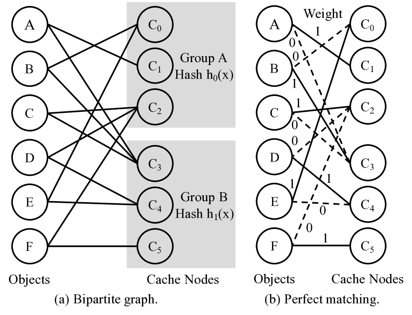
Figure 4: Example for analysis. (a) A bipartite graph constructed for the scenario in Figure 3. (b) A perfect matching for query routing when all objects have a query rate of 1, and all cache nodes have a throughput of 1.

When a perfect matching exists, it is feasible to serve all the queries by the cache nodes. We use the example in Figure 4 to illustrate this. Figure 4(a) shows the bipartite graph constructed for the scenario in Figure 3, which contains six hot objects ($A$-$F$) and six cache nodes in two layers ($C_{0}$-$C_{5}$). The edges are built based on two hash functions $h_{0}(x)$ and $h_{1}(x)$. Figure 4(b) shows a perfect matching for the case that all objects have the same query rate $r_{i}=1$ and all cache nodes have the same throughput $\widetilde{T}=1$. The number besides an edge denotes the weight of an edge, i.e., the rate of the object served by the cache node. For instance, all queries to $A$ are served by $C_{1}$. This is a simple example to illustrate the problem. In general, the query rates of the objects do not have to be the same, and the queries to one object may be served by multiple cache nodes.

Step 1: existence of a perfect matching. We first show the existence of a perfect matching for any given total rate $R$ and any query distribution $P$. We have the following lemma to demonstrate how big the total rate $R$ can be in terms of $\widetilde{T}$, for any $P$. For the full proof of Lemma 1, we refer the readers to §A.2 in the Appendix. author=Alan, color=green]We will upload report to arxiv and update the citation

Lemma 1.

Let $\alpha$ be a suitably small constant. If $k\leq m^{\beta}$ for some constant $\beta$ (i.e., $k$ and $m$ are polynomial-related) and $\max_{i}(p_{i})\cdot R\leq\widetilde{T}/2$, then for any $\epsilon>0$, there exists a perfect matching for $R=(1-\epsilon)\alpha\cdot m\widetilde{T}$ and any $P$, with high probability for sufficiently large $m$.

author=Alan, color=green]We give proof sketch of Lemma 1. Proof sketch of Lemma 1: We utilize the results and techniques developed from expander graphs and network flows. $(i)$ We first show that $G$ has the so-called expansion property with high probability. Intuitively, the property states that the neighborhood of any subset of nodes in $U$ expands, i.e., for any $S\subseteq U$, $|\Gamma(S)|\geq|S|$. It has been observed that such properties exist in a wide range of random graphs [13]. While our $G$ behaves similar to random bipartite graphs, we need the expansion property to hold for $S$ in any size, which is stricter than the standard definition (which assumes $S$ is not too large) and thus requires more delicate probabilistic techniques. $(ii)$ We then show that if a graph has the expansion property, then it has a perfect matching. This step can be viewed as a generalization of Hall’s theorem [14] in our setting. Hall’s theorem states that a balanced bipartite graph has a perfect (non-fractional) matching if and only if for any subset $S$ of the left nodes, $|\Gamma(S)|\geq|S|$. and perfect matching can be fractional. This step can be proved by the max-flow-min-cut theorem, i.e., expansion implies large cut, and then implies large matching.

Step 2: finding a perfect matching. Demonstrating the existence of a perfect matching is insufficient since it just ensures the queries can be absorbed but does not give the actual weight assignment $W$, i.e., how the cache nodes should serve queries for each $P$ to achieve $R$. This means that the system would require an algorithm to compute $W$ and an mechanism to enforce $W$. As discussed in §3.1, instead of doing so, we use the power-of-two-choices to “emulate” the perfect matching, without the need to know what the perfect matching is. The quality of the mechanism is backed by Lemma 2, which we prove using queuing theory. The detailed proof can be found in §A.3. author=Alan, color=green]We will upload report to arxiv and update the citation

Lemma 2.

If a perfect matching exists for $G$, then the power-of-two-choices process is stationary.

Stationary means that the load on the cache nodes would converge, and the system is “sustainable” in the sense that the system will never “blow up” (i.e., build up queues in a cache node and eventually drop queries) with query rate $R$.

author=Alan, color=green]We give proof sketch of Lemma 2. Proof sketch of Lemma 2: Showing this lemma requires us to use a powerful building block in query theory presented in  [15, 16]. Consider $2m$ exponential random variables with rate $\widetilde{T}_{i}>0$. Each non-empty set of cache nodes $S\subseteq[2m]$, has an associated Poisson arrival process with rate $\lambda_{S}\geq 0$ that joins the shortest queue in $S$ with ties broken randomly. For each non-empty subset $Q\subseteq[2m]$, define the traffic intensity on $Q$ as

$$\rho_{Q}=\frac{\sum_{S\subseteq Q}\lambda_{S}}{\mu_{Q}},$$

where $\mu_{Q}=\sum_{i\in Q}\widetilde{T}_{i}$. Note that the total rate at which objects served by $Q$ can be greater than the numerator of (3.2) since other requests may be allowed to be served by some or all of the cache nodes in $Q$. Let $\rho_{\max}=\max_{Q\subseteq[2m]}\{\rho_{Q}\}$. Given the result in [15, 16], if we can show $\rho_{\max}<1$, then the Markov process is positive recurrent and has a stationary distribution. In fact, our cache querying can be described as the following arrival process.

Define $D(i)=\{a_{h_{0}(i)},b_{h_{1}(i)}\}$. Let $S$ be an arbitrary subset of $\{A,B\}$. Define $\lambda_{S}$ as:

• If $S=\{a_{i},b_{j}\}$ for some $i$ and $j$, let

  $$\lambda_{S}=\sum_{i\leq k}(I(D(i)=S))p_{i}R,$$

  where $I(\cdot)$ is an indicator function that sets to $1$ if and only if its argument is true.

• Otherwise, $\lambda_{S}=0$.

Finally, we show that $\rho_{\max}$ is less than 1 (refer to §A.2) and thus the process is stationary.

Step 3: main theorem. Based on Lemma 1 and Lemma 2, we can prove that our distributed caching mechanism is able to provide a performance guarantee, despite query distribution.

Theorem 1.

Let $\alpha$ be a suitable constant. If $k\leq m^{\beta}$ for some constant $\beta$ (i.e., $k$ and $m$ are polynomial-related) and $\max_{i}(p_{i})\cdot R\leq\widetilde{T}/2$, then for any $\epsilon>0$, the system is stationary for $R=(1-\epsilon)\alpha\cdot m\widetilde{T}$ and any $P$, with high probability for sufficiently large $m$.

author=Alan, color=green]We add a quick interpretation of our analysis. Interpretation of the main theorem: As long as the query rate of a single hot object $o_{i}$ is no larger than $\widetilde{T}/2$ (e.g., half of the entire throughput in a cluster rack), DistCache can support a query rate of $\approx m\widetilde{T}$ for any query distributions to the $k$ hot objects (where $k$ can be fairly large in terms of $m$) by using the power-of-two-choices protocol to route the queries to the cached objects. The key takeaways are presented in the following section.

3.3 Remarks

Our problem isn’t a balls-in-bins problem using the original power-of-two-choices. The major difference is that our problem hashes objects into cache nodes, and queries to the same object by reusing the same hash functions, instead of using a new random source to sample two nodes for each query. In fact, without using the power-of-two-choices, the system is in non-stationary. This means that the power-of-two-choices makes a “life-or-death” improvement in our problem, instead of a “shaving off a log $n$” improvement. While we refer to the Appendix for detailed discussions, we have a few important remarks.

• Nonuniform number of cache nodes in two layers. For simplicity we use the same number of $m$ cache nodes per layer in the system. However, we can generalize the analysis to accommodate the cases of different numbers of caches nodes in two layers, as long as $\min(m_{0},m_{1})$ is sufficiently large, where $m_{0}$ and $m_{1}$ are the number of upper-layer and lower-layer cache nodes respectively. While it requires $m$ to be sufficiently large, it is not a severe restriction, because the load imbalance issue is only significant when $m$ is large.

• Nonuniform throughput of cache nodes in two groups. Although our analysis assumes the throughput of a cache node is $\widetilde{T}$, we can generalize it to accommodate the cases of nonuniform throughput by treating a cache node with a large throughput as multiple smaller cache nodes with a small throughput.

• Cache size. As long as the number of objects and the number of cache nodes are polynomially-related ($k\leq m^{\beta}$), the system is able to provide the performance guarantee. It is more relaxed than $O(m\log m)$. Therefore, by setting $k=O(m\log m)$, the cache nodes are able to absorb all queries to the hottest $O(m\log m)$ objects, making the load on the $m$ clusters balanced.

• Maximum query rate for one object. The theorem requires that the maximum query rate for one object is no bigger than half the throughput of one cache node. This is not a strict requirement for the system, because a cache node is orders of magnitude faster than a storage node.

• Performance guarantee. The system can guarantee a total throughput of $R=(1-\epsilon)\alpha\cdot mT$, which scales linearly with $m$ and $T$. In practice, $\alpha$ is close to $1$.

3.4 Use Cases

DistCache is a general solution that can be applied to scale out various storage systems (e.g., key-value stores and file systems) using different storage mediums (e.g., HDD, SDD and DRAM). We describe two use cases.

Distributed in-memory caching. Based on the performance gap between DRAMs and SSDs, a fast in-memory cache node can be used balance an SSD-based storage cluster, such as SwitchKV [10]. DistCache can scale out SwitchKV by using another layer of in-memory cache nodes to balance multiple SwitchKV clusters. While it is true that multiple in-memory cache nodes can be balanced using a faster switch-based cache node, applying DistCache obviates the need to introduce a new component (i.e., a switch-based cache) to the system. Since the queries are routed to the cache and storage nodes by the network, queries to the lower-layer cache nodes can totally bypass the upper-layer cache nodes.

Distributed switch-based caching. Many low-latency storage systems for interactive web services use more expensive in-memory designs. An in-memory storage rack can be balanced by a switch-based cache like NetCache [11], which directly caches the hot objects in the data plane of the ToR switch. DistCache can scale out NetCache to multiple racks by caching hot objects in a higher layer of the network topology, e.g., the spine layer in a two-layer leaf-spine network. As discussed in the remarks (§3.3), DistCache accommodates the cases that the number of spine switches is smaller and each spine switch is faster. As for query routing, while queries to hit the leaf cache switches need to inevitably go through the spine switches, these queries can be arbitrarily routed through any spine switches, so that the load on the spine switches can be balanced.

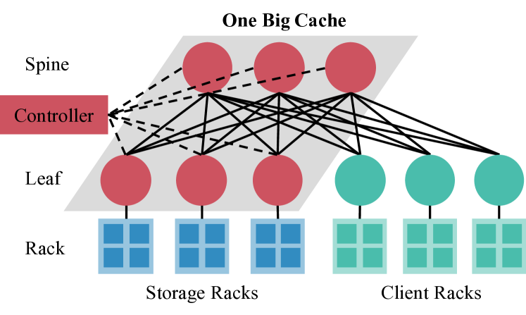
Figure 5: Architecture for distributed switch-based caching.

Note that while existing solutions (e.g., NetCache [11]) directly embeds caching in the switches which may raise concerns on deployment, another option for easier deployment is to use the cache switches as stand-alone specialized appliances that are separated from the switches in the datacenter network. DistCache can be applied to scale out these specialized switch-based caching appliances as well.

4 DistCache for Switch-Based Caching

To demonstrate the benefits of DistCache, we provide a concrete system design for the emerging switch-based caching. A similar design can be applied to other use cases as well.

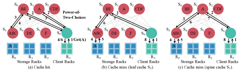
Figure 6: Query handling for $Get(A)$. $S_{6}$ uses the power-of-two-choices to decide whether to send $Get(A)$ to $S_{1}$ or $S_{3}$. (a) Upon a cache hit, the switch directly replies the query, without visiting the storage server. (b, c) Upon a cache miss, the query is forwarded to the storage server without routing detour.

4.1 System Architecture

Emerging switch-based caching, such as NetCache [11] is limited to one storage rack. We apply DistCache to switch-based caching to provide load balancing for cloud-scale key-value stores that span many racks. Figure 5 shows the architecture for a two-layer leaf-spine datacenter network.

Cache Controller. The controller computes the cache partitions, and notifies the cache switches. It updates the cache allocation under system reconfigurations, e.g., adding new racks and cache switches, and system failures; and thus updating the allocation is an infrequent task. We assume the controller is reliable by replicating on multiple servers with a consensus protocol such as Paxos [17]. The controller is not involved in handling storage queries in the data plane.

Cache switches. The cache switches provide two critical functionalities for DistCache: (1) caching hot key-value objects; (2) distributing switch load information for query routing. First, a local agent in the switch OS receives its cache partition from the controller, and manages the hot objects for its partition in the data plane. Second, the cache switches implement a lightweight in-network telemetry mechanism to distribute their load information by piggybacking in packet headers. The functionalities for DistCache are invoked by a reserved L4 port, so that DistCache does not affect other network functionalities. We use existing L2/L3 network protocols to route packets, and do not modify other network functionalities already in the switch.

ToR switches at client racks. The ToR switches at client racks provide query routing. It uses the power-of-two-choices to decide which cache switch to send a query to, and uses existing L2/L3 network protocols to route the query.

Storage servers. The storage servers host the key-value store. DistCache runs a shim layer in each storage server to integrate the in-network cache with existing key-value store software like Redis [18] and Memcached [19]. The shim layer also implements a cache coherence protocol to guarantee the consistency between the servers and cache switches.

Clients. DistCache provides a client library for applications to access the key-value store. The library provides an interface similar to existing key-value stores. It maps function calls from applications to DistCache query packets, and gathers DistCache reply packets to generate function returns.

4.2 Query Handling

A key advantage of DistCache is that it provides a distributed on-path cache to serve queries at line rate. Read queries on cached objects (i.e., cache hit) are directly replied by the cache switches, without the need to visit storage servers; read queries on uncached objects (i.e., cache miss) and write queries are forwarded to storage servers, without any routing detour. Further, while the cache is distributed, our query routing mechanism based on the power-of-two-choices ensures that the load between the cache switches is balanced.

Query routing at client ToR switches. Clients send queries via the client library, which simply translates function calls to query packets. The complexity of query routing is done at the ToR switches of the client racks. The ToR switches use the switch on-chip memory to store the loads of the cache switches. For each read query, they compare the loads of the switches that contain the queried object in their partitions, and pick the less-loaded cache switch for the query. After the cache switch is chosen, they use the existing routing mechanism to send the query to the cache switch. The routing mechanism can pick a routing path that balances the traffic in the network, which is orthogonal to this paper. Our prototype uses a mechanism similar to CONGA [20] and HULA [21] to choose the least loaded path to the cache switch.

For a cache hit, the cache switch copies the value from its on-chip memory to the packet, and returns the packet to the client. For a cache miss, the cache switch forwards the packet to the corresponding storage server that stores the queried object. Then the server processes the query and replies to the client. Figure 6 shows an example. A client in rack $R_{3}$ sends a query to read object $A$. Suppose $A$ is cached in switch $S_{1}$ and $S_{3}$, and is stored in a server in rack $R_{0}$. The ToR switch $S_{6}$ uses the power-of-two-choices to decide whether to choose $S_{1}$ or $S_{3}$. Upon a cache hit, the cache switch (either $S_{1}$ or $S_{3}$) directly replies to the client (Figure 6(a)). Upon a cache miss, the query is sent to the server. But no matter whether the leaf cache (Figure  6(b)) or the spine cache (Figure 6(c)) is chosen, there is no routing detour for the query to reach $R_{0}$ after a cache miss.

Write queries are directly forwarded to the storage servers that contain the objects. The servers implement a cache coherence protocol for data consistency as described in §4.3.

Query processing at cache switches. Cache switches use the on-chip memory to cache objects in their own partitions. In programmable switches such as Barefoot Tofino [22], the on-chip memory is organized as register arrays spanning multiple stages in the packet processing pipeline. The packets can read and update the register arrays at line rate. We uses the same mechanism as NetCache [11] to implement a key-value cache that can support variable-length values, and a heavy-hitter (HH) detector that the switch local agent uses to decide what top $k$ hottest objects in its partition to cache.

In-network telemetry for cache load distribution. We use a light-weight in-network telemetry mechanism to distribute the cache load information for query routing. The mechanism piggybacks the switch load (i.e., the total number of packets in the last second) in the packet headers of reply packets, and thus incurs minimal overhead. Specifically, when a reply packet of a query passes a cache switch, the cache switch adds its load to the packet header. Then when the reply packet reaches the ToR switch of the client rack, the ToR switch retrieves the load in the packet header to update the load stored in its on-chip memory. To handle the case that the cache load may become stale without enough traffic for piggybacking, we can add a simple aging mechanism that would gradually decrease a load to zero if the load is not updated for a long time. Note that aging is commonly supported by modern switch ASICs, but it is not supported by P4 yet, and thus is not implemented in our prototype.

4.3 Cache Coherence and Cache Update

Cache coherence. Cache coherence ensures data consistency between storage servers and cache switches when write queries update the values of the objects. The challenge is that an object may be cached in multiple cache switches, and need to be updated atomically. Directly updating the copies of an object in the cache switches may result in data inconsistency. This is because the cache switches are updated asynchronously, and during the update process, there would be a mix of old and new values at different switches, causing read queries to get different values from different switches.

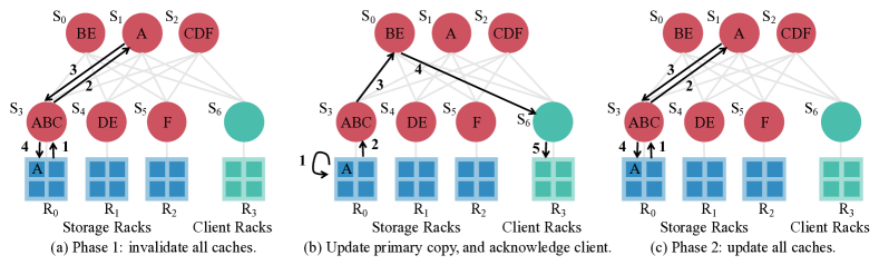
Figure 7: Cache coherence is achieved by a two-phase update protocol in DistCache. The example shows the process to handle an update to object $A$ stored in rack $R_{0}$ with the two-phase update protocol.

We leverage the classic two-phase update protocol [23] to ensure strong consistency, where the first phase invalidates all copies and the second phase updates all copies. To apply the protocol to our scenario, after receiving a write query, the storage server generates a packet to invalidate the copies in the cache switches. The packet traverses a path that includes all the switches that cache the object. The return of the invalidation packet indicates that all the copies are invalidated. Otherwise, the server resends the invalidation packet after a timeout. Figure 7(a) shows an example that the copies of object $A$ are invalidated by an invalidation packet via path $R_{0}$-$S_{3}$-$S_{1}$-$S_{3}$-$R_{0}$. After the first phase, the server can update its primary copy, and send an acknowledgment to the client, instead of waiting for the second phase, as illustrated by Figure 7(b). This optimization is safe, since all copies are invalid. Finally, in the second phase, the server sends an update packet to update the values in the cache switches, as illustrated by Figure 7(c).

Cache update. The cache update is performed in a decentralized way without the involvement of the controller. We use a similar mechanism as NetCache [11]. Specifically, the local agent in each switch uses the HH detector in the data plane to detect hot objects in its own partition, and decides cache insertions and evictions. Cache evictions can be directly done by the agent; cache insertions require the agent to contact the storage servers. Slightly different from NetCache, DistCache uses a cleaner, more efficient mechanism to unify cache insertions and cache coherence. Specifically, the agent first inserts the new object into the cache, but marks it as invalid. Then the agent notifies the server; the server updates the cached object in the data plane using phase 2 of cache coherence, and serializes this operation with other write queries. As for comparison, in NetCache, the agent copies the value from the server to the switch via the switch control plane (which is slower than the data plane), and during the copying, the write queries to the object are blocked on the server.

4.4 Failure Handling

Controller failure. The controller is replicated on multiple servers for reliability (§4.1). Since the controller is only responsible for cache allocation, even if all servers of the controller fail, the data plane is still operational and hence processes queries. The servers can be simply rebooted.

Link failure. A link failure is handled by existing network protocols, and does not affect the system, as long as the network is connected and the routing is updated. If the network is partitioned after a link failure, the operator would choose between consistency and availability, as stated by the CAP theorem. If consistency were chosen, all writes should be blocked; if availability were chosen, queries can still be processed, but cache coherence cannot be guaranteed.

ToR switch failure. The servers in the rack would lose access to the network. The switch needs to be rebooted or replaced. If the switch is in a storage rack, the new switch starts with an empty cache and uses the cache update process to populate its cache. If the switch is in a client rack, the new switch initializes the loads of all cache switches to be zero, and uses the in-network telemetry mechanism to update them with reply packets.

Other Switch failure. If the switch is not a cache switch, the failure is directly handled by existing network protocols. If the switch is a cache switch, the system loses throughput provided by this switch. If it can be quickly restored (e.g., by rebooting), the system simply waits for the switch to come back online. Otherwise, the system remaps the cache partition of the failed switch to other switches, so that the hot objects in the failed switch can still be cached, alleviating the impact on the system throughput. The remapping leverages consistent hashing [24] and virtual nodes [25] to spread the load. Finally, if the network is partitioned due to a switch failure, the operator would choose consistency or availability, similar to that of a link failure.

5 Implementation

We have implemented a prototype of DistCache to realize distributed switch-based caching, including cache switches, client ToR switches, a controller, storage servers and clients.

Cache switch. The data plane of the cache switches is written in the P4 language [26], which is a domain-specific language to program the packet forwarding pipelines of data plane devices. P4 can be used to program the switches that are based on Protocol Independent Switch Architecture (PISA). In this architecture, we can define the packet formats and packet processing behaviors by a series of match-action tables. These tables are allocated to different processing stages in a forwarding pipeline, based on hardware resources. Our implementation is compiled to Barefoot Tofino ASIC [22] with Barefoot P4 Studio software suite [27]. In the Barefoot Tofino switch, we implement a key-value cache module uses 16-byte keys, and contains 64K 16-byte slots per stage for 8 stages, providing values at the granularity of 16 bytes and up to 128 bytes without packet recirculation or mirroring. The Heavy Hitter detector module contains a Count-Min sketch [28], which has 4 register arrays and 64K 16-bit slots per array, and a Bloom filter, which has 3 register arrays and 256K 1-bit slots per array. The telemetry module uses one 32-bit register slot to store the switch load. We reset the counters in the HH detector and telemetry modules in every second. The local agent in the switch OS is written in Python. It receives cache partitions from the controller, and manages the switch ASIC via the switch driver using a Thrift API generated by the P4 compiler. The routing module uses standard L3 routing which forwards packets based on destination IP address.

Client ToR switch. The data plane of client ToR switches is also written in P4 [26] and is compiled to Barefoot Tofino ASIC [22]. Its query routing module contains a register array with 256 32-bit slots to store the load of cache switches. The routing module uses standard L3 routing, and picks the least loaded path similar to CONGA [20] and HULA [21].

Controller, storage server, and client. The controller is written in Python. It computes cache partitions and notifies the result to switch agents through Thrift API. The shim layer at each storage server implements the cache coherence protocol, and uses the hiredis library [29] to hook up with Redis [18]. The client library provides a simple key-value interface. We use the client library to generate queries with different distributions and different write ratios.

6 Evaluation

6.1 Methodology

Testbed. Our testbed consists of two 6.5Tbps Barefoot Tofino switches and two server machines. Each server machine is equipped with a 16 core-CPU (Intel Xeon E5-2630), 128 GB total memory (four Samsung 32GB DDR4-2133 memory), and an Intel XL710 40G NIC.

The goal is to apply DistCache to switch-based caching to provide load balancing for cloud-scale in-memory key-value stores. Because of the limited hardware resources we have, we are unable to evaluate DistCache at full scale with tens of switches and hundreds of servers. Nevertheless, we make the most of our testbed to evaluate DistCache by dividing switches and servers into multiple logical partitions and running real switch data plane and server software, as shown in Figure 8. Specifically, a physical switch emulates several virtual switches by using multiple queues and uses counters to rate limit each queue. We use one Barefoot Tofino switch to emulate the spine switches, and the other to emulate the leaf switches. Similarly, a physical server emulates several virtual servers by using multiple queues. We use one server to emulate the storage servers, and the other to emulate the clients. We would like to emphasize that the testbed runs the real switch data plane and runs the Redis key-value store [18] to process real key-value queries.

Performance metric. By using multiple processes and using the pipelining feature of Redis, our Redis server can achieve a throughput of 1 MQPS. We use Redis to demonstrate that DistCache can integrate with production-quality open-source software that is widely deployed in real-world systems. We allocate the 1 MQPS throughput to the emulated storage servers equally with rate limiting. Since a switch is able to process a few BQPS, the bottleneck of the testbed is on the Redis servers. Therefore, we use rate limiting to match the throughput of each emulated switch to the aggregated throughput of the emulated storage servers in a rack. We normalize the system throughput to the throughput of one emulated key-value server as the performance metric.

Workloads. We use both uniform and skewed workloads in the evaluation. The uniform workload generates queries to each object with the same probability. The skewed workload follows Zipf distribution with a skewness parameter (e.g., 0.9, 0.95, 0.99). Such skewed workload is commonly used to benchmark key-value stores [10, 30], and is backed by measurements from production systems [5, 6]. The clients use approximation techniques [10, 31] to quickly generate queries according to a Zipf distribution. We store a total of 100 million objects in the key-value store. We use Zipf-0.99 as the default query distribution to show that DistCache performs well even under extreme scenarios. We vary the skewness and the write ratio (i.e., the percentage of write queries) in the experiments to evaluate the performance of DistCache under different scenarios.

Comparison. author=Alan, color=green]explain the compared solutions quickly.To demonstrate the benefits of DistCache, we compare the following mechanisms in the experiments: DistCache, CacheReplication, CachePartition, and NoCache. As described in §2.2, CacheReplication is to replicate the hot objects to all the upper layer cache nodes, and CachePartition partitions the hot objects between nodes. In NoCache, we do not cache any objects in both layers. Note that CachePartition performs the same as only using NetCache for each rack (i.e., only caching in the ToR switches).

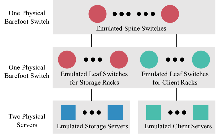
Figure 8: Evaluation setup. The testbed emulates a datacenter with a two-layer leaf-spine network by dividing switches and servers into multiple logical partitions.

(a) Throughput vs. skewness.

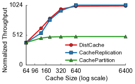
(b) Impact of cache size.

(c) Scalability.

Figure 9: System performance for read-only workloads.

6.2 Performance for Read-Only Workloads

We first evaluate the system performance of DistCache. By default, we use 32 spine switches and 32 storage racks. Each rack contains 32 servers. We populate each cache switch with 100 hot objects, so that 64 cache switches provide a cache size of 6400 objects. We use read-only workloads in this experiment, and show the impact of write queries in §6.3. We vary workload skew, cache size and system scale, and compare the throughputs of the four mechanisms under different scenarios.

Impact of workload skew. Figure 9(a) shows the throughput of the four mechanisms under different workload skews. Under the uniform workload, the four mechanisms have the same throughput, since the load between the servers is balanced and all the servers achieve their maximum throughputs. However, when the workload is skewed, the throughput of NoCache significantly decreases, because of load imbalance. The more skewed the workload is, the lower throughput NoCache achieves. CachePartition performs better than NoCache, by caching hot objects in the switches. But its throughput is still limited because of load imbalance between cache switches. CacheReplication provides the optimal throughput under read-only workloads as it replicates hot objects in all spine switches. DistCache provides comparable throughput to CacheReplication by using the distributed caching mechanism. And we will show in §6.3 that DistCache performs better than CacheReplication under writes because of low overhead for cache coherence.

Impact of cache size. Figure 9(b) shows the throughput of the three mechanisms under different cache sizes. CachePartition achieves higher throughput with more objects in the cache. Because the skewed workload still causes load imbalance between cache switches, the benefits of caching is limited for CachePartition. Some spine switches quickly become overloaded after caching some objects. As such, the throughput improvement is small for CachePartition. On the other hand, CacheReplication and DistCache gain big improvements by caching more objects, as they do not have the load imbalance problem between cache switches. The curves of CacheReplication and DistCache become flat after they achieve the saturated throughput.

Scalability. Figure 9(c) shows how the four mechanisms scale with the number of servers. NoCache does not scale because of the load imbalance between servers. Its throughput stops to improve after a few hundred servers, because the overloaded servers become the system bottleneck under the skewed workload. CachePartition performs better than NoCache as it uses the switches to absorb queries to hot objects. However, since the load imbalance still exists between the cache switches, the throughput of CachePartition stops to grow when there are a significant number of racks. CacheReplication provides the optimal solution, since replicating hot objects in all spine switches eliminates the load imbalance problem. DistCache provides the same performance as CacheReplication and scales out linearly.

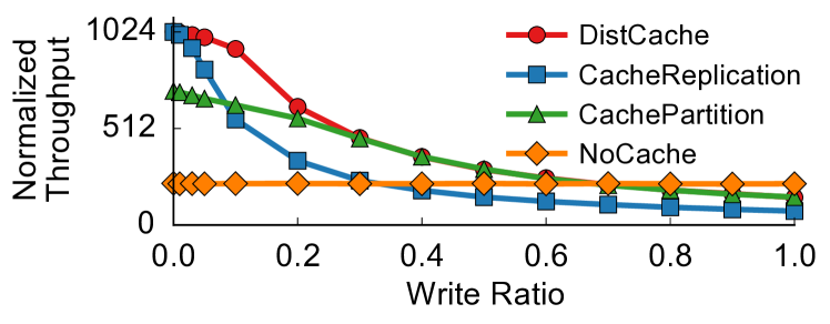
(a) Throughput vs. write ratio under Zipf-0.9 and cache size 640.

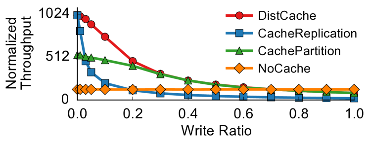
(b) Throughput vs. write ratio under Zipf-0.99 and cache size 6400.

Figure 10: Cache coherence result.

6.3 Cache Coherence

While read-only workloads provide a good benchmark to show the caching benefit, real-world workloads are usually read-intensive [5]. Write queries require the two-phase update protocol to ensure cache coherence, which $(i)$ consumes the processing power at storage servers, and $(ii)$ reduces the caching benefit as the cache cannot serve queries to hot objects that are frequently being updated. CacheReplication, while providing the optimal throughput under read-only workloads, suffers from write queries, since a write query to a cached object requires the system to update all spine switches. We use the basic setup as the previous experiment, and vary the write ratio.

Since both the workload skew and the cache size would affect the result, we show two representative scenarios. Figure 10(a) shows the scenario for Zipf-0.9 and cache size 640 (i.e., 10 objects in each cache switch). Figure  10(b) shows the scenario for Zipf-0.99 and cache size 6400 (i.e., 100 objects in each cache switch), which is more skewed and caches more objects than the scenario in Figure 10(a). NoCache is not affected by the write ratio, as it does not cache anything (and our rate limiter for the emulated storage servers assumes same overhead for read and write queries, which is usually the case for small values in in-memory key-value stores [32]). The performance of CacheReplication drops very quickly, and it is highly affected by the workload skew and the cache size, as higher skewness and bigger cache size mean more write queries would invoke the two-phase update protocol. Since DistCache only caches an object once in each layer, it has minimal overhead for cache coherence, and its throughput reduces slowly with the write ratio. The throughputs of the three caching mechanisms eventually become smaller than that of NoCache, since the servers spend extra resources on the cache coherence. Thus, in-network caching should be disabled for write-intensive workloads, which is a general guideline for many caching systems.

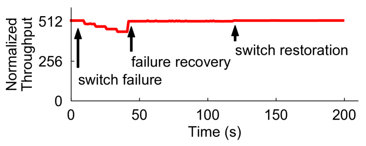
Figure 11: Time series for failure handling.

6.4 Failure Handling

We now evaluate how DistCache handles failures. Figure 11 shows the time serious of this experiment, where x-axis denotes the time and y-axis denotes the system throughput. The system starts with 32 spine switches. We manually fail four spine switches one by one. Since each spine switch provides 1/32 of the total throughput, after we fail four spine switches, the system throughput drops to about 87.5% of its original throughput. Then the controller begins a failure recovery process, by redistributing the partitions of the failed spine switches to other alive spine switches. Since the maximum throughput the system can provide drops to 87.5% due to the four failed switches, the failure recovery would have no impact if all alive spine switches were already saturated. To show the benefit of the failure recovery, we limit the sending rate to half of the maximum throughput. Therefore, after the failure recovery, the throughput can increase to the original one. Finally, we bring the four failed switches back online.

6.5 Hardware Resources

Finally, we measure the resource usage of the switches. The programmable switches we use allow developers to define their own packet formats and design the packet actions by a series of match-action tables. These tables are mapped into different stages in a sequential order, along with dedicated resources (e.g., match entries, hash bits, SRAMs, and action slots) for each stage. DistCache leverages stateful memory to maintain the cached key-value items, and minimizes the resource usage. Table 1 shows the resource usage of the switches with the caching functionality. We show all the three roles, including a spine switch, a leaf switch in a client rack, and a leaf switch in a storage rack. Compared to the baseline Switch.p4, which is a fully functional switch, adding caching only requires a small amount of resources, leaving plenty room for other network functions.

Switches	Match Entries	Hash Bits	SRAMs	Action Slots
Switch.p4	804	1678	293	503
Spine	149	751	250	98
Leaf (Client)	76	209	91	32
Leaf (Server)	120	721	252	108

Table 1: Hardware resource usage of DistCache.

7 Related Work

Distributed storage. Distributed storage systems are widely deployed to power Internet services [1, 2, 3, 4]. One trend is to move storage from HDDs and SDDs to DRAMs for high performance [19, 18, 33, 34]. Recent work has explored both hardware solutions [35, 36, 37, 38, 39, 40, 41, 42, 43, 44, 45, 46] and software optimizations [47, 48, 32, 49, 50, 51]. Most of these techniques focus on the single-node performance and are orthogonal to DistCache, as DistCache focuses on the entire system spanning many clusters.

Load balancing. Achieving load balancing is critical to scale out distributed storage. Basic data replication techniques [24, 52] unnecessarily waste storage capacity under skewed workloads. Selective replication and data migration techniques [53, 54, 55], while reducing storage overhead, increase system complexity and performance overhead for query routing and data consistency. EC-Cache [30] leverages erasure coding, but since it requires to split an object into multiple chunks, it is more suitable for large objects in data-intensive applications. Caching is an effective alternative for load balancing [9, 10, 11]. DistCache pushes the caching idea further by introducing a distributed caching mechanism to provide load balance for large-scale storage systems.

In-network computing. Emerging programmable network devices enable many new in-network applications. IncBricks [56] uses NPUs as a key-value cache. It does not focus on load balancing. NetPaxos [57, 58] presents a solution to implement Paxos on switches. SpecPaxos [59] and NOPaxos [60] use switches to order messages to improve consensus protocols. Eris [61] moves concurrency control to switches to improve distributed transactions.

8 Conclusion

We present DistCache, a new distributed caching mechanism for large-scale storage systems. DistCache leverages independent hash functions for cache allocation and the power-of-two-choices for query routing, to enable a “one big cache” abstraction. We show that combining these two techniques provides provable load balancing that can be applied to various scenarios. We demonstrate the benefits of DistCache by the design, implementation and evaluation of the use case for emerging switch-based caching.

Acknowledgments    We thank our shepherd Ken Salem and the reviewers for their valuable feedback. Liu, Braverman, and Jin are supported in part by NSF grants CNS-1813487, CRII-1755646 and CAREER 1652257, Facebook Communications & Networking Research Award, Cisco Faculty Award, ONR Award N00014-18-1-2364, DARPA/ARO Award W911NF1820267, and Amazon AWS Cloud Credits for Research Program. Ion Stoica is supported in part by NSF CISE Expeditions Award CCF-1730628, and gifts from Alibaba, Amazon Web Services, Ant Financial, Arm, CapitalOne, Ericsson, Facebook, Google, Huawei, Intel, Microsoft, Scotiabank, Splunk and VMware.

Appendix A Analysis of our algorithm

This section provides formal proofs for the lemmas and theorem presented in Section 3 of the paper.

A.1 Recap of our models and comparison

We start with reviewing notations and models setup in this paper. Recall that we have a total number of $k$ distinct objects. The arrival rate for the $i$-th object is $p_{i}$. We have a total number of $2m$ cache nodes and the processing rate for each cache node is $\widetilde{T}$. Our goal is to show that our PoT algorithm is stationary over the long run.

The bipartite graph $G=(U,V,E)$. Recall that $U=\{o_{1},o_{2},\dots,o_{k-1}\}$ is the set of objects. $A=\{a_{0},\dots,a_{m-1}\}$ and $B=\{b_{0},\dots b_{m-1}\}$ are two collections of cache nodes. Let $V=A\cup B$. We build a bipartite graph $G$ in which the left-hand side is $U$ and the right-hand side is $V$. The edge set is

$$E=\{\{o_{i},a_{j_{0}}\}\mid h_{0}(i)=j_{0}\}\cup\{\{o_{i},b_{j_{1}}\}\mid h_{1}(i)=j_{1}\}$$ (1)

Also, let $\Gamma(v)$ be the set of $v$’s neighbors in $G$ and $\Gamma(S)=\cup_{v\in S}\Gamma(v)$ for any subset $S$ of nodes.

Comparison to the balls-and-bins model. Despite the apparent similarity between the balls-and-bins model, our process is substantially different. The standard techniques used to analyze PoT algorithms are not directly applicable in our model.

Recap of the PoT algorithm in the balls-and-bins model. In the basic setting, there are a total number of $m$ bins. At each step, a new ball arrives. We use the PoT rule to determine a bin to store the new ball: we uniformly choose two random bins and place the ball to the bin with lighter load. After that, a deletion event happens: we uniformly choose a bin and remove a ball from the bin (but we do nothing if the bin is already empty). We are primarily interested in the maximum load of the bins in the stationary state.

Extensive studies of the balls-and-bins model and its “sensible variations” such as the continue time model [62, 63, 64, 65], the adversarial model [66, 67], etc. have determined that the max load of the bin is $O(\log\log n)$, in contrast to the max load of $\Theta(\log n)$ for uniform balls-in-bins algorithm (i.e., place a new ball in a randomly chosen bin).

Main difference. The main difference between our process and the PoT balls-and-bins process is that ours only has a total number of $k$ types of objects. Objects of the same type will need to “reuse” the hash functions, whereas in the balls-and-bins process, new random sources are used to choose the bins, regardless of the history (i.e., each new ball will have fresh randomness). With the new randomness, it is easier to argue that the random choices will not be bad for an extensive period of time. On the other hand, in our process we need to argue that by using only two hash functions, the system will be stable even when the number of queries is $\gg k$. In fact, the performance gap between the PoT algorithm and the uniform algorithm highlights the distinction between our process and the balls-and-bins process (proved in Section A.4).

Lemma 3.

Using the notations above, with constant probability, our system is non-stationary when we use the uniform algorithm; with $o(1)$ probability, the system is stationary when we use the PoT algorithm.

In other words, the PoT algorithm makes a “life-or-death” improvement instead of “shaving off a $\log n$” improvement: our system is provably unreliable without the PoT algorithm.

Outline of the proof. We may think of our process as a “flow problem”, in which we build a bipartite graph, where the left-hand side is the objects and the right-hand side is the cache nodes. An object connects to a cache node if and only if one of $h_{0}$ and $h_{1}$ maps the object to the cache node.

When a request for an object is handled by a cache node, there is a unit flow moving from the object to the cache node. Therefore, the objects correspond to the source/supply nodes and the cache nodes correspond to the sink nodes.

At a high level, our analysis aims to show that using the PoT algorithm in our process routes the requests according to a feasible flow. Our analysis consists of two steps.

Step 1. Show that a feasible flow exists (Section A.2). A necessary condition for the PoT algorithm to work is that a feasible solution exists for the bipartite graph flow problem. When a feasible solution does not exist, no algorithm is able to produce a stabilized system. One can also see that a feasible flow also has a natural matching interpretation (i.e., how requests are matched to the cache nodes). Therefore, we use feasible flow and perfect matching interchangeably in the rest of the analysis.

Step 2. Show that the PoT algorithm “implements” a feasible flow (Section  A.3). Building a feasible flow requires that the nodes (corresponding to objects) on the left-hand side of the bipartite graph can intelligently split the flow. Instead of performing a global computation to find a feasible flow, Step 2 demonstrates how the PoT policy, which is essentially a local algorithm, automatically finds a feasible solution.

The sections below explain each of the steps in detail.

A.2 Feasible flows/matching exists

This section explains how a perfect matching exists in $G$. Recall the definition of perfect matching:

Definition 2 (Repeat of Definition 1 in the paper.).

Let $\Gamma(v)$ be the set of neighbors of vertex $v$ in $G$. A weight assignment $W=\{w_{i,j}\in[0,\widetilde{T}]|e_{i,j}\in E\}$ is a perfect matching of $G$ if

1. $\forall o_{i}\in U:\quad\sum_{v\in\Gamma(o_{i})}w_{o_{i},v}=p_{i}\cdot R$, and

2. $\forall v\in V:\quad\sum_{u\in\Gamma(v)}w_{u,v}\leq\widetilde{T}$.

We aim to prove Lemma 4, i.e.,

Lemma 4 (Repeat of Lemma 1 in the paper).

Let $\alpha$ be a suitably small constant. If $k\leq m^{\beta}$ for some constant $\beta$ (i.e., $k$ and $m$ are polynomial-related) and $\max_{i}(p_{i})\cdot R\leq\widetilde{T}/2$, then for any $\epsilon>0$, there exists a perfect matching for $R=(1-\epsilon)\alpha\cdot m\widetilde{T}$ and any $P$, with high probability for sufficiently large $m$.

Techniques and roadmap. We develop new techniques to marry random/expansion graph theory with primal-dual properties for flows. First, we show that random bipartite graph has the so-called “expansion properties”. Then, we show that a lower bound exists on the optimal flow size by using the expansion property in the dual of the flow problem.

We decompose our analysis into two steps: Step 1a: we analyze a special case when $k=\alpha m$ and the request rates $p_{i}$ are uniform (Section A.2.1), and Step 1b: we will reduce the remaining cases to the special case (Section A.2.2).

A.2.1 Step 1a: when $k=\alpha m$ and $p_{i}$’s are uniform

This section proves the following lemma.

Lemma 5.

Let $\alpha$ be a suitably small constant. Let $k=\alpha m$, $R=(1-\epsilon)\alpha m\widetilde{T}$, and $p_{i}=\frac{(1-\epsilon)\widetilde{T}}{R}$ for all $i$. There exists a perfect matching for $G$ with high probability.

We note that (i) Lemma 4 requires $\max_{i}(p_{i})\cdot R\leq\widetilde{T}/2$ but in Lemma 5 we have $\max_{i}(p_{i})\cdot R=(1-\epsilon)\widetilde{T}$. The constant term in Lemma 4 is worse because the reduction in Section A.2.2 will introduce a constant factor loss, and (ii) because $p_{i}$’s all have the same value, we can view $G$ as an unweighted graph (however, fractional solutions are still acceptable).

We shall show that $G$ possesses the so-called “expansion property” (a notation borrowed from the spectral graph theory), and the expansion property implies the existence of a perfect matching.

Definition 3.

A bipartite graph $G=(U,V,E)$ has the expansion property if for any $S\subseteq U$, we have

$$|\Gamma(S)|\geq|S|.$$ (2)

We recall the Hall’s theorem:

Theorem 2.

[68] Let $G=(U,V,E)$ be an arbitrary unweighted bipartite graph. If $G$ has the expansion property, there exists a perfect matching in $G$.

Theorem 2 implies that to prove Lemma 5, we only need to show that $G$ has the expansion property.

Lemma 6.

Using the notations above, with diminishing probability (i.e., $o(1)$), $G$ does not have the expansion property.

Proof.

Our goal is to give an upper bound for

$$\Pr[\exists S\subseteq U:|\Gamma(S)|<|S|]\leq\sum_{S\subseteq U}\Pr[|\Gamma(S)|<|S|].$$ (3)

We divide the terms in the right-hand-side of the above inequality into two groups, each of which exhibits different combinatorics properties. Therefore, we need to use different techniques to bound the sums of the terms in these two groups.

Group 1: $|S|\geq m^{0.1}$. We aim to bound:

$$\sum_{S\subseteq V,|S|\geq m^{0.1}}\Pr[|\Gamma(S)|<|S|]=\sum_{L\geq m^{0.1}}\sum_{|S|=L}\Pr[|\Gamma(S)|<L]$$ (4)

Fix $L$ and let $S\subseteq V$ such that $|S|=L$. Let the out-going edges of $S$ be $e_{1},e_{2},...,e_{2L}$. Define an indicator random variable $\mathcal{E}_{i}$ that sets to 1 if and only if the right-end of $e_{i}$ coincides with the right-end of an $e_{j}$ for some $j<i$. We refer to $\mathcal{E}_{i}$ as a “repeat” event. Note that $|\Gamma(S)|<L$ if and only if there exists at least $L+1$ repeats. Therefore,

$$\Pr[|\Gamma(S)|<L] \leq \Pr[\sum_{i\leq 2L}\mathcal{E}_{i}\geq L+1]$$

$$\leq \Pr[\sum_{i\leq 2L}\mathcal{E}_{i}\geq L]$$

$$\leq \binom{2L}{L}\left(\frac{L}{m}\right)^{L}$$

$$\leq \left(\frac{2eL}{m}\right)^{L}$$

The last inequality uses $\binom{a}{b}\leq\left(\frac{ae}{b}\right)^{b}$ for any integers $a$ and $b$. Now, we can bound the sum of all of the terms in Group 1.

$$\sum_{L\geq m^{0.1}}\sum_{|S|=L}\Pr[|\Gamma(S)|<L]$$

$$\leq \sum_{L\geq m^{0.1}}\binom{k}{L}\left(\frac{2eL}{M}\right)^{L}$$

$$\leq m\left(\frac{\alpha me}{L}\right)^{L}\left(\frac{2eL}{m}\right)^{L}$$

$$\leq m(2e^{2}\alpha)^{m^{0.1}}\leq 1/m^{10}$$

for sufficiently large $m$ so long as $\alpha>1/(2e^{2})$.

Group 2. $|S|<m^{0.1}$. We aim to bound:

$$\sum_{L<m^{0.1}}\sum_{|S|=L}\Pr[|\Gamma(S)|<k].$$ (5)

Define $\ell_{1}\triangleq|\Gamma(S)\cap A|$ and $\ell_{2}\triangleq|\Gamma(S)\cap B|$ (recall that $A$ and $B$ are two groups of cache nodes). One can see that $|\Gamma(S)|=\ell_{1}+\ell_{2}$. Therefore, a necessary condition for $|\Gamma(S)|<|S|$ is $\ell_{1}+\ell_{2}\leq|S|-1$. For any $S\subseteq U$, we have

$$\Pr[|\Gamma(S)|<|S|] \leq \sum_{\ell_{1}+\ell_{2}\leq L-1}\binom{m}{\ell_{1}}\left(\frac{\ell_{1}}{m}\right)^{L}\binom{m}{\ell_{2}}\left(\frac{\ell_{2}}{m}\right)^{L}$$

$$\leq \sum_{\ell_{1}+\ell_{2}\leq L-1}\frac{m^{\ell_{1}+\ell_{2}}e^{\ell_{1}+\ell_{2}}(\ell_{1}\ell_{2})^{L}}{m^{2L}\ell_{1}^{\ell_{1}}\ell_{2}^{\ell_{2}}}.$$

Next, we have

$$\sum_{L\leq m^{0.1}}\sum_{|S|=L}\Pr[|\Gamma(S)|<|S|]$$

$$\leq \sum_{L\leq m^{0.1}}\binom{\alpha m}{L}\sum_{\ell_{1}+\ell_{2}\leq L-1}\frac{m^{\ell_{1}+\ell_{2}}e^{\ell_{1}+\ell_{2}}(\ell_{1}\ell_{2})^{L}}{m^{2L}\ell_{1}^{\ell_{1}}\ell_{2}^{\ell_{2}}}$$

$$\leq \sum_{L\leq m^{0.1}}\sum_{\ell_{1}+\ell_{2}\leq L-1}\frac{(\alpha e^{2})^{L}m^{\ell_{1}+\ell_{2}}}{(Lm)^{L}}\cdot\frac{(\ell_{1}\ell_{2})^{L}}{\ell_{1}^{\ell_{1}}\ell_{2}^{\ell 2}}$$

$$\leq \sum_{L<m^{0.1}}L\max_{\ell_{1}+\ell_{2}\leq L}\left\{\frac{(\alpha e^{2})^{2}m^{\ell_{1}+\ell_{2}}(\ell_{1}\ell_{2})^{L}}{(Lm)^{L}\ell_{1}^{\ell_{1}}\ell_{2}^{\ell_{2}}}\right\}$$

Next, we find an upper bound on

$$G(\ell_{1},\ell_{2})\triangleq\left\{\frac{(\alpha e^{2})^{2}m^{\ell_{1}+\ell_{2}}(\ell_{1}\ell_{2})^{L}}{(Lm)^{L}\ell_{1}^{\ell_{1}}\ell_{2}^{\ell_{2}}}\right\}.$$ (6)

First, note that when $\ell_{1}+\ell_{2}<L-1$, we can set $\ell_{1}\leftarrow\ell_{1}+1$ to increase $G(\ell_{1},\ell_{2})$.

Second, we may compute $\frac{d}{d\ell_{1}}\log(G(\ell_{1},L-1-\ell_{1}))$ to find the optimal $\ell_{1}$. We have

$$\frac{d}{d\ell_{1}}\log G(\ell_{1},L-1-\ell_{1})$$

$$= \frac{L}{(L-1-\ell_{1})\ell_{1}}-2+\log(L-1-\ell_{1})-\log(\ell_{1}).$$

We can see that the optimal value is achieved when $\ell_{1}=c_{1}L$ and $\ell_{2}=c_{2}L$ for some $c_{1},c_{2}=\Theta(1)$ and $c_{1}+c_{2}=\frac{L-1}{L}$. Thus,

$$\sum_{L<m^{0.1}}L\max_{\ell_{1}+\ell_{2}\leq L}\left\{\frac{(\alpha e^{2})^{2}m^{\ell_{1}+\ell_{2}}(\ell_{1}\ell_{2})^{L}}{(Lm)^{L}\ell_{1}^{\ell_{1}}\ell_{2}^{\ell_{2}}}\right\}$$

$$\leq \sum_{L\leq m^{0.1}}L\frac{(\alpha e^{2})^{L}}{m}\frac{(c_{1}c_{2})^{L}L^{L}}{(c_{1}^{c_{1}}c_{2}^{c_{2}}L)^{L-1}}$$

(uses $$c_{1}+c_{2}=\frac{L-1}{L}$$)

$$\leq \sum_{L\leq m^{0.1}}L\left(\frac{\alpha e^{2}c_{1}c_{2}}{c_{1}^{c_{1}}c_{2}^{c_{2}}}\right)^{L}\frac{L}{m}\leq\frac{1}{m^{0.7}}.$$

The last inequality holds when $\alpha\leq\frac{c_{1}^{c_{1}}c_{2}^{c_{2}}}{e^{2}c_{1}c_{2}}$. ∎

Finally, Lemma 6 and Lemma 2 imply Lemma 5.

A.2.2 Step 1b. Generalization

This section tackles the more general case, in which no constraints are imposed on $k$ and $p_{i}$. We first explain the intuition why the general cases can be reduced to the uniform case analyzed in Section A.2.1:

Intuition part 1 (IP1): when $k<\alpha m$. In this case, $p_{i}$ is still constrained by $\max_{i}p_{i}\cdot R\leq\widetilde{T}/2$ and therefore $p_{i}=O(\widetilde{T}/R)$. Thus, the new problem is equivalent to deleting one or more objects in the special case, and is a “strictly easier problem” (i.e., the requests are strictly smaller).

Intuition part 2 (IP2): when $k>\alpha m$. Note that when $k$ is larger than $\alpha m$, the total rate $R$ remains unchanged. This intuitively corresponds to splitting some objects into smaller ones. Consider, for example, $o_{\alpha m}$ is the splitted into $o_{\alpha m}$ and $o_{\alpha m+1}$ so that the new request rates are halved $p_{\alpha m}=p_{\alpha m+1}=\frac{p_{1}}{2}$. In this new problem $k=\alpha m+1$. Originally, there were only two hash functions handling $o_{\alpha m}$. After the splitting, four hash functions handle the same amount of requests. Note that load-balance improves when there are more hash functions.

The above intuitions assume the requests are mostly homogeneous. The most challenging case is when $k$ is large and $p_{i}$’s have a long tail. This can be viewed as a “mixture” of the above two cases: approximately $\alpha m$ objects have large $p_{i}$ (resembling the scenario addressed in IP1), and the rest of the objects have small $p_{i}$ (resembling the case in IP2). Our main technique here is to decompose a problem with heterogeneous $p_{i}$’s into subproblems so that each of them has homogeneous $p_{i}$’s. Then we argue with high probability perfect matchings exist for all the sub-problems.

Below we first describe/define basic building blocks for constructing large systems (i.e., sub-problems we are able to solve). Then we explain our decomposition analysis.

Central to our analysis is our introduction of $(\alpha,\gamma,t)$-graph family. This definition enables us to scale up (increase $k$ and/or $m$) or scale out (increase throughputs) of the basic building blocks. We say

Definition 4.

$\{G_{i}\}_{i}$ is a $(\alpha,\gamma,t)$-graph family if the graph $G_{i}=(U_{i},V_{i},E_{i})$ is a bipartite graph that represents the relationship between objects and cache nodes such that (i) there are $i$ cache nodes in each of $A$ and $B$, (ii) $|U_{i}|=\alpha i$, (iii) all the $p_{j}$’s are the same, (iv) $R\leq\gamma(1-\epsilon)mt$ for some small constant $\epsilon$; and (v) the cache node’s capacity is $t$.

A $(\alpha,\gamma,t)$-graph family is $(1-\delta)$-feasible if for sufficiently large $i$, with probability $\delta$ a perfect matching exists.

Example. Lemma 5 shows that the $(\alpha,\alpha,\widetilde{T})$-graph family is $(1-\frac{1}{m^{0.7}})$-feasible.

Different graph families may be considered as “basic building blocks”’, and we may put multiple graph families together to construct new systems that have perfect matching.

For example, suppose $(\alpha,\alpha,1)$ and $(2\alpha,\alpha,1)$ graph families ($\{G^{(1)}\}_{i}$ and $\{G^{(2)}\}_{i}$, respectively) are both $(1-\delta)$-feasible. In this case, the request rates for objects in $\{G^{(1)}\}_{i}$ are $1-\epsilon$ whereas the request rates in $\{G^{(2)}\}_{i}$ are $0.5(1-\epsilon)$. We can define an addition operation between these two families through coupling.

Coupling. There is a natural way to couple the two graphs $G^{(1)}_{m}$ and $G^{(2)}_{m}$. We may imagine that $G^{(1)}_{m}$ has $2\alpha m$ objects but the last $\alpha m$ objects have zero request rates. This allows us to couple the hash functions used in two graphs in the natural way.

Under this coupling, we can define the addition operation on $G^{(1)}_{m}$ and $G^{(i)}_{m}$. In the new system, the total number of cache nodes remains unchanged ($2m$ cache nodes). Each cache node is a “merge” of two cache nodes (one from $G^{(1)}_{m}$ and the other from $G^{(2)}_{m}$). So the new capacity is 2. There are $2\alpha m$ jobs. The request rates of half of them are $1.5(1-\epsilon)$. The other half are $0.5(1-\epsilon)$. Because $G^{(1)}_{m}$ and $G^{(2)}_{m}$ are all $1-\delta$ feasible, it becomes straightforward to compute the probability a perfect matching exists in the new system: using a union bound, this probability is $1-2\delta$.

We next walk through fundamental properties of $(\alpha,\gamma,t)$-graph families. Specifically, we show that the $(\alpha,\gamma,t)$-graph family is $(1-\delta)$-feasible as $\alpha$, $\gamma$, and $t$ scale in a suitable manner.

First, we observe that $t$ is a scale-free parameter.

Lemma 7.

If $(\alpha,\gamma,1)$-graph is $(1-\delta)$-feasible, then $(\alpha,\gamma,t)$-graph is $(1-\delta)$-feasible for any $t$.

By using a similar technique for proving Lemma 5, we also have

Lemma 8.

There exists a suitably small constant $\alpha$ such that $(\rho\alpha,\alpha,t)$-graph families are all $(1-\frac{2}{m^{0.7}})$-feasible for any $\rho\in[1,2]$.

Then we also show that when we have more objects, each of which has lower request rates, we will have a greater chance to see a perfect matching.

Lemma 9.

If $(\alpha,\gamma,t)$-graph family is $(1-\delta)$-feasible, then $(k\alpha,\gamma,t)$-graph family is also $(1-\delta)$-feasible for any positive integer $k$.

Proof.

The intuition of the proof is that we may view a cache node whose processing rate is $t$ as being no worse than a union of $k$ cache nodes, each of which has processing rate $t/k$. Specifically, we couple the following processes:

Process $G^{(1)}$: There are a total number of $\alpha m$ objects. Each of $A$ and $B$ consists of $m$ cache nodes with processing rate $t$. The request rate for each object is $(1-\epsilon)\gamma t/\alpha$.

Process $G^{(2)}$: There are a total number of $\alpha km$ objects. Each of $A$ and $B$ consists of $km$ cache nodes with processing rate $t/k$. The request rate for each object is $(1-\epsilon)\gamma t/(\alpha k)$.

The graph $G^{(2)}$ is in the $(\alpha,\gamma,t)$-family, so based on the assumption made in the lemma, with probability $(1-\delta)$ a perfect matching exists.

We can also couple $G^{(1)}$ and $G^{(2)}$ in a way that if there exists a perfect matching in $G^{(2)}$, then there exists a perfect matching in $G^{(1)}$. Specifically, we may imagine that each cache node in $G^{(1)}$ consists of $k$ smaller cache nodes in $G^{(2)}$. Let $h^{(1)}_{i}$ ($h^{(2)}_{i}$) be the hash functions used in $G^{(1)}$ ($G^{(2)}$). We shall couple $h^{(1)}_{i}$ and $h^{(2)}_{i}$ in the following way:

$$h^{(1)}_{i}(j)=\lfloor h^{(2)}_{i}(j)/k\rfloor.$$ (7)

By tying the hash functions in this way, a perfect matching in $G^{(2)}$ can be reduced to a perfect matching in $G^{(1)}$.

∎

We use Lemma 8 and Lemma 9 to prove a more general result.

Lemma 10.

There exists an $\alpha$ such that the $(\rho\alpha,\alpha,t)$-graph families are $(1-2/m^{0.7})$-feasible for all $\rho\geq 1$.

Proof.

Let $\rho^{\prime}=\rho/\lfloor\rho\rfloor\in[1,2]$. By Lemma 8, the $(\rho^{\prime}\alpha,\alpha,t)$-graph family is $(1-2/m^{0.7})$-feasible. Then By Lemma 9, the $(\rho^{\prime}\lfloor\rho\rfloor\alpha,\alpha,t)$-graph family is also $(1-2/m^{0.7})$-feasible for any $\rho$, which proves the lemma. ∎

We are now ready to prove Lemma 4.

Proof of Lemma 4.

At a high level, our goal is to decompose the matching problem into multiple smaller matching problems, each of which can be shown to have a perfect matching by using Lemmas 5 or 10.

Our analysis consists of two steps:

• Step 1. Rounding up. Our $(\alpha,\gamma,t)$-graph families require that all the request rates are uniform. Here, we need to moderately round up the request rates for each object so that we have only a small number of distinct values of request rates.

• Step 2. Decomposition. We decompose the matching problem into smaller problems that can be addressed by Lemmas 5 or 10.

Step 1. Rounding up. This is a standard trick: we construct a geometric sequence and round up each request rate to the nearest number in this sequence. Specifically, recall that $\epsilon$ is a suitably small constant. Let $\lambda=1-\epsilon/2$. Let $\lambda^{(1)}=(1-\epsilon)\widetilde{T}/2$. Let $\lambda^{(i)}=\lambda\cdot\lambda^{(i-1)}$ for $2\leq i\leq\frac{10}{\epsilon}\log n$. For each $p_{j}$, round it up to the smallest $\lambda^{(i)}/R$. We refer to the new rounded value as $\tilde{p}_{i}$.

One can check that $\sum_{i\leq k}\tilde{p}_{i}R\leq(1-c_{0}\epsilon)\alpha m\widetilde{T}$ for some constant $c_{0}$ and $\max_{i}\tilde{p}_{i}R\leq(1-\epsilon/3)\widetilde{T}/2$. One can also see that if the rounded problem has a perfect matching, the original problem also has a perfect matching. After the rounding, we have a total number of $K=\frac{10}{\epsilon}\log n$ types of request rates.

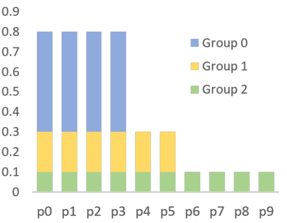
Figure 12: An illustrative example of decomposing a long-tail request distribution $\{p_{i}\}_{i}$ into three homogeneous groups. Group 0 consists of a small number of objects that have high request rates. It can be handled by Lemma 5. Group 1 and 2 consist of a large number of requests that have low request rates. They can be handled by Lemma 10.

Step 2. Decomposition. We next decompose the matching problem on $G$ into smaller sub-problems. We start with a concrete example to illustrate our high-level idea. See Fig. 12. In this example, we have a small portion of objects that have large request rates ($p_{0}$ to $p_{3}$) and a large portion of objects that have small request rates ($p_{4}$ to $p_{9}$). Now we may decompose the requests into three groups (represented by three colors). Group 0 (blue) consists of a small number of objects that have high request rates. It can be handled by Lemma 5. Group 1 and 2 (yellow and green) consist of a large number of requests that have low request rates. They can be handled by Lemma 10. We can then use a union bound to analyze the probability that perfect matchings exist for all three groups.

We now formally explain our analysis. Specifically, let

$$L_{i}=\{i:\tilde{p}_{i}\geq\lambda^{(i)}/R\}.$$

Note that $L_{1}\subseteq L_{2}\subseteq\dots\subseteq L_{K}$. Let $i^{*}$ be the largest number such that $|L_{i^{*}}|\leq\alpha m$. Next, we define the following matching sub-problems:

• $\mathcal{M}^{(0)}$: the object set is $L_{i^{*}}$. The request rate of a job $j\in L_{i^{*}}$ is $\tilde{p}^{(0)}_{j}\leftarrow\tilde{p}_{j}-\lambda^{i^{*}+1}/R$ (when $i^{*}=K$, set $\tilde{p}^{(0)}_{j}=\tilde{p}_{j}$). The processing rate of a cache node is $\widetilde{T}/2$. This corresponds to Group 0 in Fig. 12.

• $\mathcal{M}^{(i)}$ for $i>i^{*}$: the object set is $L_{i}$. The request rate of each object is $\delta^{(i)}=\lambda^{(i)}/R-\lambda^{(i+1)}/R$. The processing rate of a cache node is $\delta^{(i)}L_{i}/((1-\epsilon)m)$. This corresponds to Groups 1 and 2 in Fig. 12.

We note that we get $\tilde{p}_{j}$ if we sum up the rates for $o_{j}$ in all of the matching sub-problems. Furthermore, if we sum up cache node $i$’s processing power in all the matching sub-problem, it is $\widetilde{T}$. Therefore, if all of the matching sub-problems have perfect matching, then the original problem also has a perfect matching.

By Lemma 5, a perfect matching for $\mathcal{M}^{(0)}$ exists with probability $2/m^{0.7}$. By Lemma 10, a perfect matching for $\mathcal{M}^{(i)}$ exists with probability $2/m^{0.7}$. By using a union bound, with probability $1-2K/m^{0.7}=1-o(1/m^{0.6})$ perfect matchings exist for each subproblem. Therefore, with high probability a perfect matching exists for the original $G$. ∎

A.3 Feasible flows imply PoT is stationary (Proof of Lemma 2 in the paper)

This section proves Lemma 2 in the paper. For completeness, we repeat the lemma below.

Lemma 11 (Repeat of Lemma 2 in the paper).

If a perfect matching exists for $G$, then the power-of-two-choices process is stationary.

Proving Lemma 11 requires us to use a powerful building block presented in [15, 16]. Recall the set-up by using our notation. Consider $2m$ exponential random variables with rate $\widetilde{T}_{i}>0$. Each non-empty set of cache nodes $S\subseteq[2m]$, has an associated Poisson arrival process with rate $\lambda_{S}\geq 0$ that joins the shortest queue in $S$ with ties broken randomly. For each non-empty subset $Q\subseteq[2m]$, define the traffic intensity on $Q$ as

$$\rho_{Q}=\frac{\sum_{S\subseteq Q}\lambda_{S}}{\mu_{Q}},$$ (8)

where $\mu_{Q}=\sum_{i\in Q}\widetilde{T}_{i}$. Note that the total rate at which objects served by $Q$ can be greater than the numerator of (8) since other requests may be allowed to be served by some or all of the cache nodes in $Q$. Let $\rho_{\max}=\max_{Q\subseteq[2m]}\{\rho_{Q}\}$. We have

Theorem 3.

[15, 16] Consider the above system. If $\rho_{\max}<1$, then the Markov process is positive recurrent and has a stationary distribution $\pi$.

Proof of Lemma 11.

We need to describe our system in the language of Theorem 3. Define $D(i)=\{a_{h_{0}(i)},b_{h_{1}(i)}\}$. Let $S$ be an arbitrary subset of $\{A,B\}$. Define $\lambda_{S}$ as:

• If $S=\{a_{i},b_{j}\}$ for some $i$ and $j$, let

  $$\lambda_{S}=\sum_{i\leq k}(I(D(i)=S))p_{i}R,$$ (9)

  where $I(\cdot)$ is an indicator function that sets to $1$ if and only if its argument is true.

• Otherwise, $\lambda_{S}=0$.

One can check that the above arrival process exactly describes our cache system. We next show that $\rho_{\max}<1$.

Let $Q\subseteq A\cup B$. Let $J\subseteq[k]$ be the largest set such that for any $i\in J$, $\Gamma(i)\subseteq Q$. This implies $\Gamma(J)\subseteq Q$. On the other hand, because there is a perfect matching in $G$, we have $\sum_{i\in J}p_{i}R\leq(1-\epsilon)|\Gamma(J)|\widetilde{T}$. Therefore,

$$\rho_{Q}=\frac{\sum_{Q\subseteq A}\lambda_{Q}}{\mu_{Q}}=\frac{(1-\epsilon)\Gamma(|J|)\widetilde{T}}{\widetilde{T}|Q|}\leq(1-\epsilon).$$ (10)

Therefore, $\rho_{\max}<1$ and by Theorem 3, our process is stationary. ∎

Lemma 4 and Lemma 11 imply Theorem 4.

Theorem 4 (Main Theorem).

Let $\alpha$ be a suitable constant. If $k\leq m^{\beta}$ for some constant $\beta$ (i.e., $k$ and $m$ are polynomial-related) and $\max_{i}(p_{i})\cdot R\leq\widetilde{T}/2$, then for any $\epsilon>0$, the system is stationary for $R=(1-\epsilon)\alpha\cdot m\widetilde{T}$ and any $P$, with high probability for sufficiently large $m$.

A.4 Proof of Lemma 3

This section proves that when only one hash function is used, with constant probability our system is not stationary. Without loss of generality, let $p_{i}R=1$ for all $i$, $\widetilde{T}>1$ be an arbitrary constant, and $k=m$. Let $h:[k]\rightarrow A\cup B$ be the hash function we use. We continue to build a bipartite graph, in which the node set is $U\cup V$ ($U=\{o_{i}\}_{i\leq k}$ and $V=A\cup B$). Also, an edge $\{u,v\}$ is added if and only if $h(u)=v$. We shall show that with constant probability there exists an $S$ such that

$$|S|>\widetilde{T}|\Gamma(S)|.$$ (11)

This means even when $\widetilde{T}$ is a constant times larger than $p_{i}R$, with constant probability requests from $S$ cannot be properly handled (i.e., the request rate is larger than the processing rate). We can use a standard anti-concentration result. Specifically we shall show that for a fixed $v$:

$$\Pr\left[\exists S:|S|=\widetilde{T}+1\wedge\left(h(s)=v\mbox{ for all }s\in S\right)\right]=\Omega(1)$$ (12)

Define a sequence of indicator random variables $\{X_{i}\}_{i\leq k}$ such that $X_{i}=1$ if and only if $h(i)=v$. Note that

$$\Pr\left[\sum_{i\leq k}X_{i}=\widetilde{T}+1\right]=\binom{k}{\widetilde{T}+1}\left(\frac{1}{m}\right)^{\tilde{T}+1}\geq\left(\frac{1}{\widetilde{T}+1}\right)^{\widetilde{T}+1}=\Omega(1).$$ (13)

This shows (12) and completes the proof of Lemma 3.

References

- [1] S. Ghemawat, H. Gobioff, and S.-T. Leung, “The Google file system,” in ACM SOSP, October 2003.
- [2] G. DeCandia, D. Hastorun, M. Jampani, G. Kakulapati, A. Lakshman, A. Pilchin, S. Sivasubramanian, P. Vosshall, and W. Vogels, “Dynamo: Amazon’s highly available key-value store,” in ACM SOSP, October 2007.
- [3] D. Beaver, S. Kumar, H. C. Li, J. Sobel, P. Vajgel, et al., “Finding a needle in Haystack: Facebook’s photo storage.,” in USENIX OSDI, October 2010.
- [4] R. Nishtala, H. Fugal, S. Grimm, M. Kwiatkowski, H. Lee, H. C. Li, R. McElroy, M. Paleczny, D. Peek, P. Saab, D. Stafford, T. Tung, and V. Venkataramani, “Scaling Memcache at Facebook,” in USENIX NSDI, April 2013.
- [5] B. Atikoglu, Y. Xu, E. Frachtenberg, S. Jiang, and M. Paleczny, “Workload analysis of a large-scale key-value store,” in ACM SIGMETRICS, June 2012.
- [6] B. F. Cooper, A. Silberstein, E. Tam, R. Ramakrishnan, and R. Sears, “Benchmarking cloud serving systems with YCSB,” in ACM Symposium on Cloud Computing, June 2010.
- [7] Q. Huang, H. Gudmundsdottir, Y. Vigfusson, D. A. Freedman, K. Birman, and R. van Renesse, “Characterizing load imbalance in real-world networked caches,” in ACM SIGCOMM HotNets Workshop, October 2014.
- [8] J. Jung, B. Krishnamurthy, and M. Rabinovich, “Flash crowds and denial of service attacks: Characterization and implications for CDNs and web sites,” in WWW, May 2002.
- [9] B. Fan, H. Lim, D. G. Andersen, and M. Kaminsky, “Small cache, big effect: Provable load balancing for randomly partitioned cluster services,” in ACM Symposium on Cloud Computing, October 2011.
- [10] X. Li, R. Sethi, M. Kaminsky, D. G. Andersen, and M. J. Freedman, “Be fast, cheap and in control with SwitchKV,” in USENIX NSDI, March 2016.
- [11] X. Jin, X. Li, H. Zhang, R. Soulé, J. Lee, N. Foster, C. Kim, and I. Stoica, “NetCache: Balancing key-value stores with fast in-network caching,” in ACM SOSP, October 2017.
- [12] M. Mitzenmacher, “The power of two choices in randomized load balancing,” IEEE Transactions on Parallel and Distributed Systems, October 2001.
- [13] S. P. Vadhan et al., “Pseudorandomness,” Foundations and Trends® in Theoretical Computer Science, vol. 7, no. 1–3, pp. 1–336, 2012.
- [14] J. Nešetril, “Graph theory and combinatorics,” Lecture Notes, Fields Institute, pp. 11–12, 2011.
- [15] S. Foss and N. Chernova, “On the stability of a partially accessible multi-station queue with state-dependent routing,” Queueing Systems, 1998.
- [16] R. D. Foley and D. R. McDonald, “Join the shortest queue: stability and exact asymptotics,” Annals of Applied Probability, pp. 569–607, 2001.
- [17] L. Lamport, “The part-time parliament,” ACM Transactions on Computer Systems, May 1998.
- [18] “Redis data structure store.” https://redis.io/.
- [19] “Memcached key-value store.” https://memcached.org/.
- [20] M. Alizadeh, T. Edsall, S. Dharmapurikar, R. Vaidyanathan, K. Chu, A. Fingerhut, V. T. Lam, F. Matus, R. Pan, N. Yadav, and G. Varghese, “CONGA: Distributed congestion-aware load balancing for datacenters,” in ACM SIGCOMM, August 2014.
- [21] N. Katta, M. Hira, C. Kim, A. Sivaraman, and J. Rexford, “Hula: Scalable load balancing using programmable data planes,” in ACM SOSR, March 2016.
- [22] “Barefoot Tofino.” https://www.barefootnetworks.com/technology/#tofino.
- [23] P. A. Bernstein, V. Hadzilacos, and N. Goodman, Concurrency Control and Recovery in Database Systems. Addison-Wesley Longman Publishing Co., Inc., 1986.
- [24] D. Karger, E. Lehman, T. Leighton, R. Panigrahy, M. Levine, and D. Lewin, “Consistent hashing and random trees: Distributed caching protocols for relieving hot spots on the world wide web,” in ACM Symposium on Theory of Computing, May 1997.
- [25] F. Dabek, M. F. Kaashoek, D. Karger, R. Morris, and I. Stoica, “Wide-area cooperative storage with CFS,” in ACM SOSP, October 2001.
- [26] P. Bosshart, D. Daly, G. Gibb, M. Izzard, N. McKeown, J. Rexford, C. Schlesinger, D. Talayco, A. Vahdat, G. Varghese, and D. Walker, “P4: Programming protocol-independent packet processors,” SIGCOMM CCR, July 2014.
- [27] “Barefoot P4 Studio.” https://www.barefootnetworks.com/products/brief-p4-studio/.
- [28] G. Cormode and S. Muthukrishnan, “An Improved Data Stream Summary: The Count-min Sketch and Its Applications,” J. Algorithms, 2005.
- [29] “Hiredis: Redis library.” https://redis.io/.
- [30] K. V. Rashmi, M. Chowdhury, J. Kosaian, I. Stoica, and K. Ramchandran, “EC-Cache: Load-balanced, low-latency cluster caching with online erasure coding,” in USENIX OSDI, November 2016.
- [31] J. Gray, P. Sundaresan, S. Englert, K. Baclawski, and P. J. Weinberger, “Quickly generating billion-record synthetic databases,” in ACM SIGMOD, May 1994.
- [32] H. Lim, D. Han, D. G. Andersen, and M. Kaminsky, “MICA: A holistic approach to fast in-memory key-value storage,” in USENIX NSDI, April 2014.
- [33] “Amazon DynamoDB accelerator (DAX).” https://aws.amazon.com/dynamodb/dax/.
- [34] J. Ousterhout, A. Gopalan, A. Gupta, A. Kejriwal, C. Lee, B. Montazeri, D. Ongaro, S. J. Park, H. Qin, M. Rosenblum, S. Rumble, R. Stutsman, and S. Yang, “The RAMCloud storage system,” ACM Transactions on Computer Systems, August 2015.
- [35] M. Blott, K. Karras, L. Liu, K. A. Vissers, J. Bär, and Z. István, “Achieving 10Gbps line-rate key-value stores with FPGAs,” in USENIX HotCloud Workshop, June 2013.
- [36] S. R. Chalamalasetti, K. Lim, M. Wright, A. AuYoung, P. Ranganathan, and M. Margala, “An FPGA Memcached appliance,” in ACM/SIGDA FPGA, February 2013.
- [37] K. Lim, D. Meisner, A. G. Saidi, P. Ranganathan, and T. F. Wenisch, “Thin servers with smart pipes: Designing SoC accelerators for Memcached,” in ACM/IEEE ISCA, June 2013.
- [38] B. Li, Z. Ruan, W. Xiao, Y. Lu, Y. Xiong, A. Putnam, E. Chen, and L. Zhang, “KV-Direct: High-performance in-memory key-value store with programmable NIC,” in ACM SOSP, October 2017.
- [39] A. Kalia, M. Kaminsky, and D. G. Andersen, “Using RDMA efficiently for key-value services,” in ACM SIGCOMM, August 2014.
- [40] A. Kalia, M. Kaminsky, and D. G. Andersen, “Design guidelines for high performance RDMA systems,” in USENIX ATC, June 2016.
- [41] A. Dragojević, D. Narayanan, M. Castro, and O. Hodson, “FaRM: Fast remote memory,” in USENIX NSDI, April 2014.
- [42] S. Li, K. Lim, P. Faraboschi, J. Chang, P. Ranganathan, and N. P. Jouppi, “System-level integrated server architectures for scale-out datacenters,” in IEEE/ACM MICRO, December 2011.
- [43] P. Lotfi-Kamran, B. Grot, M. Ferdman, S. Volos, O. Kocberber, J. Picorel, A. Adileh, D. Jevdjic, S. Idgunji, E. Ozer, et al., “Scale-out processors,” in ACM/IEEE ISCA, June 2012.
- [44] A. Gutierrez, M. Cieslak, B. Giridhar, R. G. Dreslinski, L. Ceze, and T. Mudge, “Integrated 3D-stacked server designs for increasing physical density of key-value stores,” in ACM ASPLOS, March 2014.
- [45] S. Novakovic, A. Daglis, E. Bugnion, B. Falsafi, and B. Grot, “Scale-out NUMA,” in ACM ASPLOS, March 2014.
- [46] S. Li, H. Lim, V. W. Lee, J. H. Ahn, A. Kalia, M. Kaminsky, D. G. Andersen, O. Seongil, S. Lee, and P. Dubey, “Architecting to achieve a billion requests per second throughput on a single key-value store server platform,” in ACM/IEEE ISCA, June 2015.
- [47] D. G. Andersen, J. Franklin, M. Kaminsky, A. Phanishayee, L. Tan, and V. Vasudevan, “FAWN: A fast array of wimpy nodes,” in ACM SOSP, October 2009.
- [48] X. Li, D. G. Andersen, M. Kaminsky, and M. J. Freedman, “Algorithmic improvements for fast concurrent cuckoo hashing,” in EuroSys, April 2014.
- [49] B. Fan, D. G. Andersen, and M. Kaminsky, “MemC3: Compact and concurrent memcache with dumber caching and smarter hashing,” in USENIX NSDI, April 2013.
- [50] V. Vasudevan, M. Kaminsky, and D. G. Andersen, “Using vector interfaces to deliver millions of IOPS from a networked key-value storage server,” in ACM Symposium on Cloud Computing, October 2012.
- [51] H. Lim, B. Fan, D. G. Andersen, and M. Kaminsky, “SILT: A memory-efficient, high-performance key-value store,” in ACM SOSP, October 2011.
- [52] F. Dabek, M. F. Kaashoek, D. Karger, R. Morris, and I. Stoica, “Wide-area cooperative storage with CFS,” in ACM SOSP, October 2001.
- [53] Y. Cheng, A. Gupta, and A. R. Butt, “An in-memory object caching framework with adaptive load balancing,” in EuroSys, April 2015.
- [54] M. Klems, A. Silberstein, J. Chen, M. Mortazavi, S. A. Albert, P. Narayan, A. Tumbde, and B. Cooper, “The Yahoo!: Cloud datastore load balancer,” in CloudDB, October 2012.
- [55] R. Taft, E. Mansour, M. Serafini, J. Duggan, A. J. Elmore, A. Aboulnaga, A. Pavlo, and M. Stonebraker, “E-Store: Fine-grained elastic partitioning for distributed transaction processing systems,” in VLDB, November 2014.
- [56] M. Liu, L. Luo, J. Nelson, L. Ceze, A. Krishnamurthy, and K. Atreya, “IncBricks: Toward in-network computation with an in-network cache,” in ACM ASPLOS, April 2017.
- [57] H. T. Dang, D. Sciascia, M. Canini, F. Pedone, and R. Soulé, “NetPaxos: Consensus at network speed,” in ACM SOSR, June 2015.
- [58] H. T. Dang, M. Canini, F. Pedone, and R. Soulé, “Paxos made switch-y,” SIGCOMM CCR, April 2016.
- [59] D. R. K. Ports, J. Li, V. Liu, N. K. Sharma, and A. Krishnamurthy, “Designing distributed systems using approximate synchrony in data center networks,” in USENIX NSDI, May 2015.
- [60] J. Li, E. Michael, N. K. Sharma, A. Szekeres, and D. R. Ports, “Just say NO to Paxos overhead: Replacing consensus with network ordering,” in USENIX OSDI, November 2016.
- [61] J. Li, E. Michael, and D. R. Ports, “Eris: Coordination-free consistent transactions using in-network concurrency control,” in ACM SOSP, October 2017.
- [62] M. J. Luczak, C. McDiarmid, et al., “On the power of two choices: balls and bins in continuous time,” The Annals of Applied Probability, 2005.
- [63] M. J. Luczak and C. McDiarmid, “On the maximum queue length in the supermarket model,” The Annals of Probability, pp. 493–527, 2006.
- [64] M. Bramson, Y. Lu, and B. Prabhakar, “Randomized load balancing with general service time distributions,” in ACM SIGMETRICS performance evaluation review, ACM, 2010.
- [65] M. Bramson, Y. Lu, and B. Prabhakar, “Asymptotic independence of queues under randomized load balancing,” Queueing Systems, vol. 71, no. 3, pp. 247–292, 2012.
- [66] R. Cole, A. Frieze, B. M. Maggs, M. Mitzenmacher, A. W. Richa, R. Sitaraman, and E. Upfal, “On balls and bins with deletions,” in International Workshop on Randomization and Approximation Techniques in Computer Science, pp. 145–158, Springer, 1998.
- [67] Y. Azar, A. Z. Broder, A. R. Karlin, and E. Upfal, “Balanced allocations,” SIAM journal on computing, vol. 29, no. 1, pp. 180–200, 1999.
- [68] B. Bollobás, Modern graph theory, vol. 184. Springer Science & Business Media, 2013.