Phase boundary location with information-theoretic entropy in tensor renormalization group flows
Abstract
We present a simple and efficient tensor network method to accurately locate phase boundaries of two-dimensional classical lattice models. The method utilizes only the information-theoretic (von Neumann) entropy of quantities that automatically arise along tensor renormalization group [Phys. Rev. Lett. 12, 120601 (2007)] flows of partition functions. We benchmark the method against theoretically known results for the square-lattice -state Potts models, which includes first-order, weakly first-order, and continuous phase transitions, and find good agreement in all cases. We also compare against previous Monte Carlo results for the frustrated square lattice Ising model and find good agreement.
I Introduction
Tensor networks serve as a powerful ansätze for many-body quantum wavefunctions and many-body classical partition functions Cirac and Verstraete (2009); Orús (2014). Algorithms to find tensor network representations of quantum wavefunctions or classical partition functions entail discarding the irrelevant portions of Hilbert space or state space to find representations that are numerically efficient. The pioneering example of this is the density matrix renormalization group (DMRG) White (1992), devised for wavefunctions of one-dimensional quantum lattices, but also applicable to two-dimensional classical lattices Nishino (1995) through the well known quantum-classical correspondence. The first developments explicitly for two-dimensional classical lattices were transfer matrix-based algorithms Nishino and Okunishi (1996, 1997); Murg et al. (2005), followed by the block spin-like tensor renormalization group (TRG) Levin and Nave (2007) algorithm. Variations of TRG were then developed Xie et al. (2009); Gu and Wen (2009); Zhao et al. (2010); Xie et al. (2012); Evenbly and Vidal (2015); Yang et al. (2017); Bal et al. (2017); Morita et al. (2018); Hauru et al. (2018); Evenbly (2018); Harada (2018); Nakamura et al. (2019); Iino et al. (2019a); Adachi et al. (2019) for better accuracy and enhanced capability, such as applicability in higher dimensions . These tensor network algorithms do not suffer from the notorious sign problem that sometimes arises in Monte Carlo.
Tensor network methods can be used to locate and characterize phase boundaries of classical lattice models either via the type of thermodynamic analysis that is done with Monte Carlo or through non-thermodynamic analysis. Thermodynamic analysis entails calculation of higher order moments of physical quantities, which is a highly non-trivial task with tensor networks. Nevertheless, a recent work Morita and Kawashima (2019) showed how to accomplish this to high accuracy with higher order TRG (HOTRG) Xie et al. (2012) and used it to compute the phase transition temperature, transition order (i.e. first-order vs. continuous), and critical exponents for the -,-,-,-, and -state Potts models on the square lattice. Non-thermodynamic analysis can be done through computations with the fixed point tensors from TRG-type algorithms. These fixed point tensors encode the degeneracy of the phase in a very simple way Gu and Wen (2009), and an abrupt change in the degeneracy indicates a phase transition. This approach has been used, for example, with HOTRG to compute the critical temperature of the 2-state Potts model on the simple cubic lattice to very high precision Shun et al. (2014). Additionally, computations of the central charge and scaling dimensions from the fixed point tensors Gu and Wen (2009); Evenbly and Vidal (2015); Hauru et al. (2018) can locate continuous phase transitions and yield their critical exponents (exceptional cases may be continuous transitions that do not have conformal invariance, such as the phase transition in the -state Potts model on the square lattice).
In this work we deal with an alternative non-thermodynamic quantity for phase boundary location: von Neumann entropy. A few recent works Krčmár and Šamaj (2015); Krcmar et al. (2016); Krčmár et al. (2016); Huang et al. (2017) have utilized von Neumann entropy to locate phase boundaries of 2d classical lattices with the corner transfer matrix renormalization group (CTMRG) algorithm Nishino and Okunishi (1996, 1997), but we are not aware of any works that do so with TRG. Here we explain the straightforward use of von Neumann entropy for phase boundary location of 2d classical lattice models with the TRG algorithm. In contrast to the thermodynamic approach, the von Neumann entropy TRG method presented here is vastly simpler because it does not require computation of higher order moments. In contrast to the phase degeneracy method, the von Neumann entropy TRG method does not require coarse graining deep into the thermodynamic limit and does not require encoding of symmetries (numerical instability can blur the transition point in the phase degeneracy method if symmetries are not encoded, as seen in Ref. Yang and Xie, 2016). In contrast to the approach of computing central charge, which locates only continuous transitions, the von Neumann entropy TRG method can locate both first-order and continuous transitions.
On the other hand, the von Neumann entropy TRG method is specific to only two-dimensional lattices and can not characterize the phase boundary, whereas the other approaches (both thermodynamic and non-thermodynamic) are applicable in higher dimensions as well and can characterize the phase boundary (except for the phase degeneracy method).
The use of von Neumann entropy as a signal for 2d classical phase transitions comes through the well known correspondence between (1+1)d quantum and 2d classical models. In particular, the phase transition of a 2d classical model coincides with a phase transition of the same type in a corresponding (1+1)d quantum model. In a (1+1)d quantum model the von Neumann entropy of the reduced density matrix of a (sufficiently large) contiguous subsystem is maximal at a phase transition, and this entropy maximum also marks a phase transition in the corresponding 2d classical model. TRG simulations of 2d classical models have direct access to the von Neumann entropy of the corresponding (1+1)d quantum system, and can therefore use it to locate the phase boundaries of 2d classical models. We show below that tuning 2d classical models to maximize this von Neumann entropy in TRG simulations gives the location of their phase transitions to good accuracy.
In the following sections we first review the relevant theoretical background of TRG (sections II. and III.), then describe the implementation of our method (section IV.). In section V. we benchmark against the theoretically known transition temperatures of the square lattice q-state Potts models, which exhibit different transitions (depending on the value of ): first-order, weakly first-order, and continuous. In section VI. we apply our method to the frustrated Ising model on the square lattice and compare our results to previously published Monte Carlo results.
II TRG flows of partition functions near phase boundaries
Partition functions of two-dimensional classical lattices can be represented as contractions of two-dimensional networks of tensors Levin and Nave (2007) where each tensor corresponds to a few lattice sites. An example given in Ref. Levin and Nave, 2007 for the partition function () of a honeycomb lattice model is
| (1) |
where is a three-leg tensor corresponding to three microscopic degrees of freedom. The TRG algorithm begins with a few (or even just one) tensors at the UV scale and applies a succession of steps, each of which simultaneously grows and coarse grains the lattice. The growth of the lattice is exponential in the number of TRG steps, which makes calculation of the thermodynamic partition function computationally feasible: after tens of TRG steps, a single tensor represents many degrees of freedom rather than just a few, and tracing over only one or a few tensor(s) becomes sufficient to approximate the partition function in the thermodynamic limit. For example, in the case of a monopartite square lattice the TRG algorithm may start with a single tensor corresponding to a system size of , and after TRG steps end with a single tensor that corresponds to a system size of .
TRG coarse graining entails an information compression scheme, based on the singular value decomposition, that in many cases allows the coarse grained tensors of a partition function to have low compression error (a.k.a. “truncation error”) while still keeping the dimension of their indices (a.k.a. “bond dimension”) within computationally feasible limits. More precisely, the minimum bond dimension required for maintaining low truncation error grows with each coarse graining step in the early part of the TRG flow of a partition function, but saturates to a finite value when the coarse graining approaches the correlation length of the system. Near criticality, however, the correlation length diverges, and TRG breaks down in the sense that the minimum bond dimension required for maintaining low truncation error grows without saturating at a computationally feasible value. TRG coarse graining to the thermodynamic limit with low truncation error therefore becomes computationally prohibitive for partition functions near criticality (i.e. the tensors required become too large). Similarly, the finite but very large correlation lengths that are a hallmark of weakly first-order phase transitions can also make low-loss TRG flows to the thermodynamic limit computationally prohibitive. Crucially, our method of using TRG flows to locate phase boundaries does not require the TRG flows to always maintain low truncation error. Therefore, TRG flows with bond dimension () fixed at computationally modest sizes are sufficient for our method.
III TRG von Neumann entropy as ground state entanglement entropy
The correspondence between 2d classical and (1+1)d quantum systems means that a theoretical understanding of our method can be gained by considering the entanglement properties of ground states of (1+1)d quantum spin chains and their finite- tensor network representations. We discuss here the specific case of matrix product states (MPSs) Fannes et al. (1992); Östlund and Rommer (1995); Perez-Garcia et al. (2007); Vidal (2007); Orus and Vidal (2008) due to the availability of relevant results. The wavefunction of a (1+1)d quantum spin chain with sites may be represented as a MPS: , where the are tensors of dimension , is the dimension of spin at site , and is again referred to as the “bond dimension”.
For a bipartite quantum system in a pure state, the subsystems and may each still have a mixed (i.e. uncertain) state due to quantum correlations (i.e. entanglement) between and . The resulting “entanglement entropy” of subsystem is defined as . It is useful to consider the entanglement entropy of a contiguous subblock in both infinite and finite (1+1)d quantum spin chains. In the ground state of the chain, the entanglement entropy of such a contiguous subblock, as well as its MPS representation, exhibits universal properties near and at criticality Amico et al. (2008); Holzhey et al. (1994); Osterloh et al. (2002); Vidal et al. (2003); Latorre et al. (2003); Calabrese and Cardy (2004); Refael and Moore (2004); Tagliacozzo et al. (2008); Pollmann et al. (2009); Pirvu et al. (2012).
In the ground state of an infinite chain, the entanglement entropy of the infinite half-chain diverges near criticality as , where is the correlation length of the system. In an infinite MPS (iMPS) Vidal (2007); Orus and Vidal (2008) representation, however, the finite bond dimension causes the entanglement entropy to saturate to a finite maximum near the critical point (the distance from the critical point goes to zero as ) Tagliacozzo et al. (2008); Pollmann et al. (2009). The finite of iMPSs also leads to a -dependent universal scaling behavior of local observables, which enables a “finite entanglement scaling” (FES) Tagliacozzo et al. (2008); Pollmann et al. (2009) analysis analogous to the well known finite size scaling (FSS) analysis.
A finite-length () contiguous subblock of an infinite chain has entanglement entropy constant in off criticality and logarithmic in at criticality (for sufficiently large ) Vidal et al. (2003). This behavior also occurs for contiguous subblocks of sufficiently large finite chains in the ground stateVidal et al. (2003), but with a modification: at criticality the entanglement entropy grows logarithmically over a finite range of but then saturates and starts to decrease after reaching half the chain length due to the finiteness of the system. Thus, in either case (infinite chain or large, finite chain), there is a range of for which the entanglement entropy is maximal at the critical point. For finite chains, MPS representations with sufficiently large can reproduce this behavior. Further, it was shown for the case of periodic boundary conditions that such finite MPSs exhibit a crossover (as a function of and system size) between regimes where either FSS or FES is valid Pirvu et al. (2012). For the entanglement entropy this means a crossover between and .
The upshot is that in all of the above cases of (1+1)d quantum systems and their finite-entanglement (i.e. finite-) tensor network representations, the critical point can be approximately identified with the parameter value that maximizes the entanglement entropy. The same must also be true for first order transitions if the correlation length on both sides of the transition is maximal at the transition (this is intuitively expected to be the usual case). In the present work, we wish to investigate how well this information-theoretic way of locating phase boundaries of (1+1)d quantum systems translates to two-dimensional classical lattice models via the quantum-classical correspondence in TRG.
The quantum-classical correspondence in the case of TRG is such that the tensor at each step in a TRG flow of a classical 2d partition function corresponds to a representation of a (1+1)d quantum ground state imagined to live on the boundary of the classical system Levin and Nave (2007). The gap of the corresponding classical and quantum systems is the same, and each tensor leg corresponds to a contiguous subblock of the periodic (1+1)d quantum system whose size grows exponentially in the number of TRG steps. For the example of a square lattice, this can be summarized as
| (2) |
where is the boundary ground state wavefunction, is the TRG tensor, and is a pure state of the contiguous subblock corresponding to tensor leg . Here it is manifest that the TRG tensor encodes the entanglement between the subblocks of the (1+1)d quantum chain. At each TRG step, a singular value spectrum results from a singular value decomposition of the reshaped tensor, e.g. . Therefore, the von Neumann entropy of the singular value spectrum at a particular TRG step corresponds to the entanglement entropy of a contiguous subblock of the boundary (1+1)d quantum system at that step. This is also the case for HOTRG Ueda et al. (2014).
Near criticality the finite value of results in a crossover in the behavior of the entanglement entropy growth from linear to constant in TRG step (see Fig. (1) for an example); this is qualitatively like the FSS to FES crossover known for periodic MPS Pirvu et al. (2012) and also the scaling crossover near criticality in CTMRG Nishino et al. (1996). Further, Ueda et al. Ueda et al. (2014) quantitatively confirmed the presence of FES in HOTRG flows of the critical partition function of the Ising model in the region after the crossover. We therefore make the following conjecture: FES is generically valid after the von Neumann entropy crossover in TRG flows of critical partition functions. Combining this conjecture with the behavior of entanglement in the FES regime of (1+1)d quantum systems (i.e., that the entanglement entropy is maximal very close to the true critical point) and the quantum-classical correspondence, we arrive at the simple idea behind the method described in the next section: the maximum of the TRG von Neumann entropy after the crossover gives a good approximation for the location of the phase boundary. The benchmarks below validate this idea.
In passing, we note here the result in Ref. Pirvu et al., 2012 that ground states of critical MPS rings in the FES regime correctly capture local universal properties in spite of having vanishing overlap with the true ground states.
| q-state Potts | |||||
| sq. lattice | () | () | () | () | () |
| TRG, =20 | 0.99795 | 0.90948 | 0.85037 | 0.80901 | 0.70553 |
| TRG, =30 | 0.99453 | 0.91140 | 0.85099 | 0.80657 | 0.70257 |
| TRG, =40 | 0.99494 | 0.91083 | 0.85193 | 0.80716 | 0.70247 |
| theory | 0.99497 | 0.91024 | 0.85153 | 0.80761 | 0.70123 |
| - sq. lattice | |||||
|---|---|---|---|---|---|
| TRG, =20 | 1.946 | 1.256 | 0.868 | 0.973 | 1.568 |
| TRG, =30 | 1.943 | 1.255 | 0.868 | 0.972 | 1.568 |
| TRG, =40 | 1.944 | 1.255 | 0.867 | 0.972 | 1.568 |
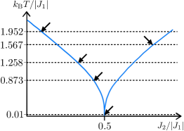
| Monte Carlo | 1.952 | 1.258 | 0.873 | 0.95 | 1.567 |
IV Method
In our simulations we always find that the von Neumann entropy of singular values in TRG flows of partition functions reaches a maximum along the flow just before plateauing in the FES regime (see Fig.(1) for an example). Though larger lattice sizes (i.e. more TRG steps) intuitively give better results in the absence of truncation error, it is of no benefit to grow the lattice further once the FES regime is reached since the numerical correlation length has then reached the limit set by . The number of TRG steps after which the FES regime is entered is model- and -dependent, but the generic existence of the entropy peak along TRG flows allows us to accommodate all scenarios in an algorithmically simple way. Therefore, we implement our method around the peak value of the von Neumann entropy along individual TRG flows: for the TRG flow at a given temperature and we simply monitor the von Neumann entropy along the flow and find the step after which the von Neumann entropy decreases for five consecutive steps. We then record the von Neumann entropy at step as the peak entropy value for that temperature and . As illustrated in Fig. (1), for a given the temperature that maximizes this peak entropy is designated as the transition temperature. For first order transitions there is no emergent criticality or FES regime, but we may still use the same method by assuming that the physical correlation length is maximal at the phase boundary. We show with benchmarks below that this method works very well with only modest for continuous, weakly first order, and regular first order phase transitions, and that it works for both unfrustrated and frustrated systems.
V Benchmarks: Potts models
Here we benchmark our method with theoretical results for the -state Potts models on the square lattice Wu (1982); the Hamiltonian is
| (3) |
where , is the Kronecker delta function, denotes nearest neighbors, and . For the phase transition is theoretically known as continuous, and for it is first-order. For the phase transition is very weakly first order (i.e. has a finite but very large correlation length); the strength of the first order nature increases with (i.e. the correlation length becomes smaller).
In Table 1 we compare the transition temperatures () from our method (to precision ) with the theoretically known values . Further data at more values of is shown in Fig. (2). Our method performs very well with only moderate values of , and the numerical results (nonmonotonically) approach the theoretical results as increases.
VI Application: J1-J2 Ising model
Here we compare our method’s results with previous Monte Carlo results for the (frustrated) Ising model on the square lattice. The Hamiltonian is
| (4) |
where , denotes nearest neighbors, and denotes next nearest (i.e. diagonal) neighbors.
In Table 2 we compare the transition temperatures from our method with the values obtained in the Monte Carlo studies in Ref. Kalz et al., 2008; Murtazaev et al., 2015. With only moderate values of , the results from our method match closely with the Monte Carlo results. Further comparison between the methods is provided in Fig. (3), which displays the computed transition values of at fixed temperatures with different values of . As illustrated in the schematic phase diagram in Fig. (4), this model has more than one phase transition in over a range of temperatures; we arbitrarily choose one at each temperature for the data in Fig. (3).
VII Summary
By leveraging the (1+1)d quantum to 2d classical correspondence known to exist in TRG and what is already known about the behavior of the entanglement entropy in MPSs near criticality, we have shown that the von Neumann entropy of the singular values that arise in computationally efficient TRG flows of partition functions near first-order, weakly first-order, and continuous phase transitions can provide an accurate location of phase transitions in spite of the presence of large truncation errors.
Due to it’s combination of simplicity, efficiency, and accuracy, the method presented here has the potential to become a standard tool for locating phase boundaries of 2d classical lattice models. Though restricted to only phase boundary location of two-dimensional classical systems, the method presented here is extremely fast, much simpler than performing thermodynamic analysis, does not require encoding of symmetries, and is applicable to both first-order and continuous phase transitions.
We note that the method described here can also work with two-dimensional HOTRG instead of TRG; it is an avenue for further investigation to see if using this method with HOTRG instead of TRG can yield better accuracy at similar cost.
VIII Acknowledgements
AAG acknowledges discussions with Kai-Hsin Wu and Glen Evenbly. This work is supported by the MOST in Taiwan through Grants No. 107-2112-M-002 -016 -MY3, and 105-2112-M-002 -023 -MY3.
*
Appendix A
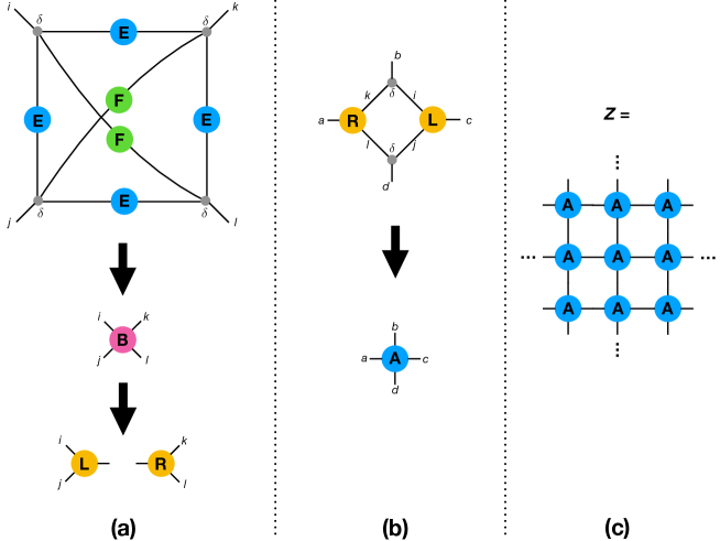
Tensor network representations of classical partition functions are not unique Zhao et al. (2010). We detail here the particular representation that we use for the TRG flows of the partition function of the frustrated Ising model of Eq. (4). The representation is that of a single repeated tensor, whose construction was pointed out by Evenbly Evenbly .
We illustrate the construction in Fig.(5). The strategy is to contract a single plaquette of the partition function on the real lattice and then split and reshape it so that the next nearest neighbor interactions of the original plaquette become nearest neighbor interactions between the new tensors. Let E and F be symmetric matrices with elements and , where is the kronecker delta function. Matrices E and F along with 4-index kronecker delta functions form the tensor network at the top of Fig. (5a), where each leg represents an index of the associated tensor and connected legs represent a contraction of the corresponding tensors over the corresponding indices. The network is first contracted into tensor and then reshaped into the symmetric matrix and split with an eigendecomposition into matrices and such that , where and (Einstein summation convention applies). and are then reshaped into three-index tensors and contracted with 3-index kronecker delta functions to yield the single repeated tensor for the partition function: .
References
- Cirac and Verstraete (2009) J. I. Cirac and F. Verstraete, J. Phys. A 42, 504004 (2009).
- Orús (2014) R. Orús, Ann. Phys. (N. Y.) 349, 117 (2014).
- White (1992) S. R. White, Phys. Rev. Lett. 69, 2863 (1992).
- Nishino (1995) T. Nishino, J. Phys. Soc. Jpn. 64, 3598 (1995).
- Nishino and Okunishi (1996) T. Nishino and K. Okunishi, J. Phys. Soc. Jpn. 65, 891 (1996).
- Nishino and Okunishi (1997) T. Nishino and K. Okunishi, J. Phys. Soc. Jpn. 66, 3040 (1997).
- Murg et al. (2005) V. Murg, F. Verstraete, and J. I. Cirac, Phys. Rev. Lett. 95, 057206 (2005).
- Levin and Nave (2007) M. Levin and C. P. Nave, Phys. Rev. Lett. 99, 120601 (2007).
- Xie et al. (2009) Z.-Y. Xie, H.-C. Jiang, Q. N. Chen, Z.-Y. Weng, and T. Xiang, Phys. Rev. Lett. 103, 160601 (2009).
- Gu and Wen (2009) Z.-C. Gu and X.-G. Wen, Phys. Rev. B 80, 155131 (2009).
- Zhao et al. (2010) H.-H. Zhao, Z.-Y. Xie, Q. N. Chen, Z.-C. Wei, J. W. Cai, and T. Xiang, Phys. Rev. B 81, 174411 (2010).
- Xie et al. (2012) Z.-Y. Xie, J. Chen, M.-P. Qin, J. W. Zhu, L.-P. Yang, and T. Xiang, Phys. Rev. B 86, 045139 (2012).
- Evenbly and Vidal (2015) G. Evenbly and G. Vidal, Phys. Rev. Lett. 115, 180405 (2015).
- Yang et al. (2017) S. Yang, Z.-C. Gu, and X.-G. Wen, Phys. Rev. Lett. 118, 110504 (2017).
- Bal et al. (2017) M. Bal, M. Mariën, J. Haegeman, and F. Verstraete, Phys. Rev. Lett. 118, 250602 (2017).
- Morita et al. (2018) S. Morita, R. Igarashi, H.-H. Zhao, and N. Kawashima, Phys. Rev. E 97, 033310 (2018).
- Hauru et al. (2018) M. Hauru, C. Delcamp, and S. Mizera, Phys. Rev. B 97, 045111 (2018).
- Evenbly (2018) G. Evenbly, Phys. Rev. B 98, 085155 (2018).
- Harada (2018) K. Harada, Phys. Rev. B 97, 045124 (2018).
- Nakamura et al. (2019) Y. Nakamura, H. Oba, and S. Takeda, Phys. Rev. B 99, 155101 (2019).
- Iino et al. (2019a) S. Iino, S. Morita, and N. Kawashima, arXiv preprint arXiv:1905.02351 (2019a).
- Adachi et al. (2019) D. Adachi, T. Okubo, and S. Todo, arXiv preprint arXiv:1906.02007 (2019).
- Morita and Kawashima (2019) S. Morita and N. Kawashima, Comput. Phys. 236, 65 (2019).
- Shun et al. (2014) W. Shun, X. Zhi-Yuan, C. Jing, B. Normand, and X. Tao, Chin. Phys. Lett. 31, 070503 (2014).
- Krčmár and Šamaj (2015) R. Krčmár and L. Šamaj, Phys. Rev. E 92, 052103 (2015).
- Krcmar et al. (2016) R. Krcmar, A. Gendiar, and T. Nishino, Phys. Rev. E 94, 022134 (2016).
- Krčmár et al. (2016) R. Krčmár, A. Gendiar, and T. Nishino, arXiv preprint arXiv:1612.07611 (2016).
- Huang et al. (2017) C.-Y. Huang, T.-C. Wei, and R. Orús, Phys. Rev. B 95, 195170 (2017).
- Yang and Xie (2016) L.-P. Yang and Z.-Y. Xie, J. Phys. Soc. Jpn. 85, 104602 (2016).
- Fannes et al. (1992) M. Fannes, B. Nachtergaele, and R. F. Werner, Comm. Math. Phys. 144, 443 (1992).
- Östlund and Rommer (1995) S. Östlund and S. Rommer, Phys. Rev. Lett. 75, 3537 (1995).
- Perez-Garcia et al. (2007) D. Perez-Garcia, F. Verstraete, M. Wolf, and J. Cirac, Quantum Inf. Comput. 7 (2007).
- Vidal (2007) G. Vidal, Phys. Rev. Lett. 98, 070201 (2007).
- Orus and Vidal (2008) R. Orus and G. Vidal, Phys. Rev. B 78, 155117 (2008).
- Amico et al. (2008) L. Amico, R. Fazio, A. Osterloh, and V. Vedral, Rev. Mod. Phys. 80, 517 (2008).
- Holzhey et al. (1994) C. Holzhey, F. Larsen, and F. Wilczek, Nucl. Phys. B 424, 443 (1994).
- Osterloh et al. (2002) A. Osterloh, L. Amico, G. Falci, and R. Fazio, Nature 416, 608 (2002).
- Vidal et al. (2003) G. Vidal, J. I. Latorre, E. Rico, and A. Kitaev, Phys. Rev. Lett. 90, 227902 (2003).
- Latorre et al. (2003) J. I. Latorre, E. Rico, and G. Vidal, arXiv preprint quant-ph/0304098 (2003).
- Calabrese and Cardy (2004) P. Calabrese and J. Cardy, J. Stat. Mech. Theory Exp. 2004, P06002 (2004).
- Refael and Moore (2004) G. Refael and J. E. Moore, Phys. Rev. Lett. 93, 260602 (2004).
- Tagliacozzo et al. (2008) L. Tagliacozzo, T. R. de Oliveira, S. Iblisdir, and J. I. Latorre, Phys. Rev. B 78, 024410 (2008).
- Pollmann et al. (2009) F. Pollmann, S. Mukerjee, A. M. Turner, and J. E. Moore, Phys. Rev. Lett. 102, 255701 (2009).
- Pirvu et al. (2012) B. Pirvu, G. Vidal, F. Verstraete, and L. Tagliacozzo, Phys. Rev. B 86, 075117 (2012).
- Ueda et al. (2014) H. Ueda, K. Okunishi, and T. Nishino, Phys. Rev. B 89, 075116 (2014).
- Nishino et al. (1996) T. Nishino, K. Okunishi, and M. Kikuchi, Phys. Lett. A 213, 69 (1996).
- Buddenoir and Wallon (1993) E. Buddenoir and S. Wallon, J. Phys. A 26, 3045 (1993).
- Iino et al. (2019b) S. Iino, S. Morita, N. Kawashima, and A. W. Sandvik, J. Phys. Soc. Jpn. 88, 034006 (2019b).
- Murtazaev et al. (2015) A. Murtazaev, M. Ramazanov, and M. Badiev, Physica B 476, 1 (2015).
- Kalz et al. (2008) A. Kalz, A. Honecker, S. Fuchs, and T. Pruschke, Eur. Phys. J. 65, 533 (2008).
- Wu (1982) F.-Y. Wu, Rev. Mod. Phys. 54, 235 (1982).
- (52) G. Evenbly, private communication .