Anomaly matching in QCD thermal phase transition

Abstract

We study an ’t Hooft anomaly of massless QCD at finite temperature. With the imaginary baryon chemical potential at the Roberge-Weiss point, there is a $\mathbb{Z}_{2}$ symmetry which can be used to define confinement. We show the existence of a mixed anomaly between the $\mathbb{Z}_{2}$ symmetry and the chiral symmetry, which gives a strong relation between confinement and chiral symmetry breaking. The anomaly is a parity anomaly in the QCD Lagrangian reduced to three dimensions. It is reproduced in the chiral Lagrangian by a topological term related to Skyrmion charge, matching the anomaly before and after QCD phase transition. The effect of the imaginary chemical potential is suppresssed in the large $N$ expansion, and we discuss implications of the ’t Hooft anomaly matching for the nature of QCD phase transition with and without the imaginary chemical potential. Arguments based on universality alone are disfavored, and a first order phase transition may be the simplest possibility if the large $N$ expansion is qualitatively good.

1 Introduction and summary

QCD phase transition is a very important problem in high energy physics and cosmology, and it is also an extremely difficult problem. Until recently, there were almost no rigorous results about the nature of QCD phase transition. There have been mainly two approaches to the problem. One approach is numerical lattice simulation, and the other is by assuming effective theories of Landau-Ginzburg type based on the argument of universality.

At the point of physical quark masses, what is often said is that the QCD phase transition is cross-over, i.e., there is no definite phase transition and thermodynamic quantities behave smoothly as the temperature is changed. This is suggested by lattice simulations Aoki:2006we ; Bhattacharya:2014ara . It is also suggested by the argument of universality in chiral symmetry breaking $\mathrm{SU}(2)_{L}\times\mathrm{SU}(2)_{R}\to\mathrm{SU}(2)$ if the up and down quark masses $m_{u,d}$ are regarded as small (but nonzero) and the strange quark mass $m_{s}$ as heavy Pisarski:1983ms . In that case, the phase transition may be second order in the limit $m_{u,d}\to 0$ if we assume universality, and the small nonzero $m_{u,d}$ change the transition from second order to cross-over.

However, because of difficulties of numerical lattice simulation in small quark mass region, it is important to study the overall picture rather than just specific quark masses, and perform consistency checks to really firmly establish such results. For example, we can vary quark masses to study the so-called Columbia plot of QCD phase diagram, and we can also vary the baryon chemical potential as a continuous parameter. See e.g. Fukushima:2010bq for a review.

In fact, some of the results obtained so far are still not consistent with each other. For example, it is not yet clear whether the phase transition is first order or second order in the chiral limit $m_{u,d}\to 0$ or $m_{u,d,s}\to 0$, and different studies give different results. For brief summaries of the current situation, see e.g. Ding:2017giu ; Aoki-san .

Because of the above situation, it is important to find rigorous results which do not rely on numerical simulation or the assumption of universality. It was difficult to obtain such rigorous results in finite temperature cases. However, a great progress was made towards this direction in Gaiotto:2017yup . In that work, pure Yang-Mills theories with the topological $\theta$ angle at $\theta=\pi$ have been studied at finite temperature, by using ’t Hooft anomalies. By an ’t Hooft anomaly, we mean an anomaly of global symmetries which exists if the global symmetries are gauged, as in the ’t Hooft’s consideration of chiral symmetry breaking by using the anomaly of the chiral symmetry $\mathrm{SU}(N_{f})_{L}\times\mathrm{SU}(N_{f})_{R}$ (see Weinberg:1996kr for a standard textbook). In Gaiotto:2017yup , a very subtle ’t Hooft anomaly was found which survives even in finite temperature case, and it is used to severely constrain the nature of the phase transition in pure Yang-Mills theories. Such subtle ’t Hooft anomalies are very useful for four dimensional gauge theories Tachikawa:2016xvs ; Yamazaki:2017ulc ; Tanizaki:2017bam ; Komargodski:2017smk ; Shimizu:2017asf ; Kikuchi:2017pcp ; Gaiotto:2017tne ; Poppitz:2017ivi ; DiVecchia:2017xpu ; Kitano:2017jng ; Tanizaki:2017qhf ; Yamazaki:2017dra ; Tanizaki:2017mtm ; Cherman:2017dwt ; Guo:2017xex ; Draper:2018mpj ; Seiberg:2018ntt ; Shifman:2018yxh ; Ritz:2018mce ; Aitken:2018kky ; Aitken:2018mbb ; Anber:2018iof ; Argurio:2018uup ; Cordova:2018acb ; Anber:2018jdf ; Tanizaki:2018wtg ; Bi:2018xvr ; Yamaguchi:2018xse ; Anber:2018xek ; Bashmakov:2018ghn ; Hsin:2018vcg ; Wan:2018zql as well as lower dimensional strongly coupled systems.

For the applications to QCD phase transition, the most relevant anomaly found so far is the one discussed in Shimizu:2017asf (see also Tanizaki:2017qhf ; Tanizaki:2017mtm ). In the present paper, we further study this direction (but the present paper is more elementary and self-contained). In Shimizu:2017asf , a subtle anomaly has been found when there is an imaginary baryon chemical potential $\mu_{B}$ at a special value $\mu_{B}=\pi$, where $\mu_{B}$ is normalized to be dimensionless. Finite temperature QCD with imaginary chemical potential is a very important subject, and has been studied extensively (e.g. Alford:1998sd ; Lombardo:1999cz ; deForcrand:2002hgr ; deForcrand:2003vyj ; deForcrand:2006pv ; deForcrand:2008vr ; DElia:2002tig ; DElia:2004ani ; Azcoiti:2005tv ; Chen:2004tb ; Karbstein:2006er ; Cea:2006yd ; Cea:2007vt ; Cea:2010md ; Wu:2006su ; Nagata:2011yf ; Giudice:2004se ; DElia:2007bkz ; Cea:2009ba ; Alexandru:2013uaa ; Cea:2012ev ; Conradi:2007be ; DElia:2009pdy ; Takaishi:2010kc ; Cea:2014xva ; Cea:2015cya ; Bonati:2014kpa ; Bonati:2014rfa ; Bonati:2015bha ; Bellwied:2015rza ; Gunther:2016vcp ; DElia:2016jqh ; Bornyakov:2017upg ; Andreoli:2017zie ; Greensite:2014isa ; Greensite:2014cxa ; Takahashi:2014rta ; Takahashi:2014ofa ; Greensite:2017qfl ; DElia:2009bzj ; deForcrand:2010he ; Bonati:2010gi ; Philipsen:2014rpa ; Wu:2013bfa ; Wu:2014lsa ; Nagata:2014fra ; Kashiwa:2016vrl ; Kashiwa:2015tna ; Bonati:2016pwz ; Makiyama:2015uwa ; Philipsen:2015eya ; Cuteri:2015qkq ; Bonati:2018fvg ; Kouno:2009bm ; Sakai:2009dv ; Sasaki:2011wu ; Kouno:2011zu ; Aarts:2010ky ; Rafferty:2011hd ; Morita:2011eu ; Kashiwa:2011td ; Pagura:2011rt ; Scheffler:2011te ; Kashiwa:2013rm ; Kashiwa:2012xm ; Filothodoros:2016txa ; Filothodoros:2018pdj ). One of the motivations is that it is related by analytic continuation to real chemical potential, and imaginary chemical potential has no sign problem. However, the imaginary chemical potential is also useful for the study of QCD phase transition at zero chemical potential. As mentioned above, it is helpful to study the overall picture of phase diagram when various parameters are changed, such as $\mu_{B}$. In particular, the value $\mu_{B}=\pi$ is special because confinement and deconfinement can be precisely defined at that value. In $\mathrm{SU}(N_{c})$ Yang-Mills theory without quarks, the confinement/deconfinement is characterized by the center symmetry ${\mathbb{Z}}_{N_{c}}$. A well-known problem in QCD with fundamental quarks is that the center symmetry is explicitly broken and hence confinement/deconfinement is not precisely defined. However, at the special value $\mu_{B}=\pi$, there is a ${\mathbb{Z}}_{2}$ symmetry Roberge:1986mm which can be used as a kind of center symmetry as we will review later in this paper. We denote this symmetry as ${\mathbb{Z}}_{2}^{\rm center}$ and call the point $\mu_{B}=\pi$ as the Roberge-Weiss point Roberge:1986mm . Then the phase structure is much more clear at this value because of the well-definedness of confinement/deconfinement. See also Kouno:2012zz ; Sakai:2012ika ; Kouno:2013zr ; Kouno:2013mma ; Poppitz:2013zqa ; Iritani:2015ara ; Kouno:2015sja ; Hirakida:2016rqd ; Hirakida:2017bye ; Cherman:2017tey ; Tanizaki:2017qhf ; Tanizaki:2017mtm for flavor-dependent imaginary chemical potential in which the center symmetry is preserved.

Intuitively the reason that confinement is well-defined at $\mu_{B}=\pi$ is explained as follows, whose details will be discussed later in this paper. Let $L$ be the Polyakov loop operator (i.e., Wilson loop operator in the direction of the thermal circle $S^{1}$). This operator $L$ includes $\mu_{B}$ (regarded as a background field for baryon symmetry) as well as the usual color gauge fields. The Polyakov loop may be considered as a world-line of a probe quark (or “heavy quark” put by hand). Its vacuum expectation value behaves, intuitively, as

$$\left\langle{L}\right\rangle\sim\exp(-\beta E_{q}+i\mu_{B}B)$$ (1)

where $\beta=T^{-1}$ is the inverse temperature, $E_{q}$ is the energy of a probe quark (up to “bare mass of the heavy quark”), $B$ is the baryon number of the probe quark (see below for more discussion), and $\mu_{B}$ is the imaginary chemical potential. In the absence of dynamical quarks, confinement means that an isolated probe quark has an infinite energy $E_{q}\to+\infty$ and hence confinement (deconfinement) is defined by $\left\langle{L}\right\rangle=0$ ($\left\langle{L}\right\rangle\neq 0$). However, in the presence of dynamical quarks, the probe quark is screened by dynamical anti-quarks as in the right of Figure 1 and hence $\left\langle{L}\right\rangle\neq 0$ in any phase. However, let us introduce $\mu_{B}=\pi$. Then the phase of $\left\langle{L}\right\rangle$ is given by $\exp(i\pi B)$. For gauge invariant composites as in the right of Figure 1 the total baryon number is integer and hence $\exp(i\pi B)$ is real. On the other hand, for an isolated quark as in the left of Figure 1 the baryon number is not integer, $B=1/N_{c}$, and hence $\exp(i\pi B)$ is imaginary. Therefore, the imaginary part $\mathop{\mathrm{Im}}\left\langle{L}\right\rangle$ is a good order parameter for a criterion of confinement.

Figure 1: How to define confinement. Here $Q_{\rm probe}$ is the probe quark representing the Polyakov loop, and $\overline{q}$ is a dynamical anti-quark. In the confinement phase (Right) the baryon number $B$ is always integer and hence $e^{i\pi B}=\pm 1\in{\mathbb{R}}$, while in the deconfinement phase (Left) it is not necessarily integer because quarks have fractional baryon number $1/N_{c}$ and hence $e^{i\pi B}\in{\mathbb{C}}$.

Now, there is a ${\mathbb{Z}}_{2}$ symmetry which changes the direction of the thermal circle $S^{1}$. Then the Polyakov loop is complex conjugated,

$${\mathbb{Z}}_{2}^{\rm center}:L\to L^{*}.$$ (2)

The $\mathop{\mathrm{Im}}\left\langle{L}\right\rangle$ is the order parameter of this ${\mathbb{Z}}_{2}^{\rm center}$. We define confinement phase as a phase in which ${\mathbb{Z}}_{2}^{\rm center}$ is unbroken, $\left\langle{L}\right\rangle=0$.

We will show in this paper that there is a mixed anomaly between the ${\mathbb{Z}}_{2}^{\rm center}$ symmetry and the chiral symmetry $\mathrm{SU}(N_{f})_{L}\times\mathrm{SU}(N_{f})_{R}$. This gives a direct strong relation between confinement and chiral symmetry breaking, extending the original results of ’t Hooft. See Figure 2.

Figure 2: Mixed anomaly between ${\mathbb{Z}}_{2}^{\rm center}$ and $\mathrm{SU}(N_{f})_{L}\times\mathrm{SU}(N_{f})_{R}$ at finite temperature.

The existence of the ’t Hooft anomaly puts severe constraints on the nature of phase transition, because the theory at any temperature must have the same ’t Hooft anomaly. Such an anomaly immediately excludes the simplest scenario of chiral phase transition based on the universality alone, at least at the Roberge-Weiss point $\mu_{B}=\pi$. Moreover, we will see that the effect of $\mu_{B}$ is only sub-leading in the large $N$ expansion. Therefore, the constraints obtained at $\mu_{B}=\pi$ may have important implications even for the case $\mu_{B}=0$ if the large $N$ expansion is qualitatively good. Large $N$ analysis is at least qualitatively good in QCD at zero temperature, so we may hope that it is also useful at finite temperature.

Summary of the results.

Let us summarize the results of the present paper, which confirm and strengthen the results in Shimizu:2017asf by more elementary arguments.

In section 2 we see that finite temperature QCD at the Roberge-Weiss point $\mu_{B}=\pi$ has a parity anomaly Redlich:1983dv ; Niemi:1983rq ; AlvarezGaume:1984nf ; Witten:2016cio between ${\mathbb{Z}}_{2}^{\rm center}$ (which will be realized as a parity symmetry in three dimensions after the reduction on the thermal circle $S^{1}$) and the chiral symmetry $\mathrm{SU}(N_{f})_{L}\times\mathrm{SU}(N_{f})_{R}$. This is the anomaly shown in Figure 2.

In section 3 we will reproduce the parity anomaly in the effective theory of pions (i.e. chiral Lagrangian) from the Wess-Zumino-Witten term. In particular, a term related to the topological charge of Skyrmions plays the crucial role. The importance of the Skyrmion charge in QCD anomalies was already recognized in Witten:1983tw ; Witten:1983tx , and it was used in more sophisticated way in a recent work Tanizaki:2018wtg at zero temperature.

In section 4 we will discuss implications of the anomaly for possible scenarios of QCD phase transition at $\mu_{B}=\pi$, and extrapolate that discussion to $\mu_{B}=0$ in the large $N$ expansion. At $\mu_{B}=\pi$, a first order transition may be the most natural scenario of $\mathrm{SU}(N_{c})$ QCD phase transition for generic flavor numbers $N_{f}\mathop{}_{\textstyle\sim}^{\textstyle<}N_{c}$, although the anomaly itself allows more exotic scenarios such as a deconfined $\mathrm{U}(1)$ gauge field, chiral symmetry breaking in deconfining phase, and so on. If it is a first order transition, then the result may be unchanged for $\mu_{B}=0$ as far as the large $N$ analysis is qualitatively valid.

2 Anomaly of QCD Lagrangian

We consider the standard QCD-like theories with general color and flavor numbers $N_{c}$ and $N_{f}$. It is the $\mathrm{SU}(N_{c})$ gauge theory with $N_{f}$ flavors of quark fields $\Psi$ in the fundamental representation of $\mathrm{SU}(N_{c})$. The Lagrangian is

$${\cal L}=-\frac{1}{2g^{2}}\operatorname{tr}_{c}((F_{C})_{\mu\nu}(F_{C})^{\mu\nu})+\overline{\Psi}\gamma^{\mu}D_{\mu}\Psi,$$ (3)

where $(F_{C})_{\mu\nu}$ is the field strength of the $\mathrm{SU}(N_{c})$ gauge fields $A_{C}$, $\gamma^{\mu}$ are gamma matrices with $\{\gamma_{\mu},\gamma_{\nu}\}=2\delta_{\mu\nu}$ in Euclidean space, and $D_{\mu}=\partial_{\mu}+(A_{C})_{\mu}$ is the covariant derivative.

The full symmetry group of this theory is a bit complicated, and in this paper we use only partial information. Including the gauge as well as some of the global symmetry groups, the quark fields are acted by

$$H=[\mathrm{SU}(N_{c})\times\mathrm{SU}(N_{f})_{L}\times\mathrm{SU}(N_{f})_{R}\times\mathrm{U}(1)_{V}]/{\mathscr{D}}.$$ (4)

Here $\mathrm{SU}(N_{f})_{L}$ and $\mathrm{SU}(N_{f})_{R}$ are the standard chiral symmetry. They act on the left and right handed quarks ${\psi}_{L}=\frac{(1+\gamma_{5})}{2}\Psi$ and $\overline{\psi}_{R}=\frac{(1-\gamma_{5})}{2}\Psi$ as $\psi_{L}\mapsto g_{L}\psi_{L}$ and $\overline{\psi}_{R}\mapsto g_{R}\overline{\psi}_{R}$ for $g_{L,R}\in\mathrm{SU}(N_{f})_{L,R}$. The $\mathrm{U}(1)_{V}$ acts as $\Psi\to g_{V}\Psi$ where $g_{V}\in\mathrm{U}(1)_{V}$ is a phase factor $|g_{V}|=1$. The ${\mathscr{D}}$ is a subgroup of the center of the group

$${\mathscr{D}}\subset\mathrm{SU}(N_{c})\times\mathrm{SU}(N_{f})_{L}\times\mathrm{SU}(N_{f})_{R}\times\mathrm{U}(1)_{V}$$ (5)

which acts trivially on the quark fields $\Psi$. More explicitly it is generated by elements $c_{1},c_{2}\in{\mathscr{D}}$ given by

$$c_{1} =(e^{2\pi i/N_{c}},1,1,e^{-2\pi i/N_{c}}),$$ (6)

$$c_{2} =(1,e^{2\pi i/N_{f}},e^{2\pi i/N_{f}},e^{-2\pi i/N_{f}}).$$ (7)

These $c_{1}$ and $c_{2}$ act trivially on the quarks and gluons.

The symmetry group which acts on gauge invariant operators can be obtained by omitting the gauge group $\mathrm{SU}(N_{c})$ in $H$. We get

$$G=[\mathrm{SU}(N_{f})_{L}\times\mathrm{SU}(N_{f})_{R}\times\mathrm{U}(1)_{B}]/{\mathscr{C}}.$$ (8)

Here, the baryon number symmetry $\mathrm{U}(1)_{B}$ is given by

$$\mathrm{U}(1)_{B}=\mathrm{U}(1)_{V}/{\mathbb{Z}}_{N_{c}}$$ (9)

where ${\mathbb{Z}}_{N_{c}}$ is generated by the element $c_{1}$ above. The quark fields have charge $1/N_{c}$ under this $\mathrm{U}(1)_{B}$. The ${\mathscr{C}}={\mathbb{Z}}_{N_{f}}$ is generated by $c_{2}$. In terms of $\mathrm{U}(1)_{B}$ rather than $\mathrm{U}(1)_{V}$, it is given by

$$c^{\prime}_{2}=(e^{2\pi i/N_{f}},e^{2\pi i/N_{f}},e^{-2\pi iN_{c}/N_{f}})\in\mathrm{SU}(N_{f})_{L}\times\mathrm{SU}(N_{f})_{R}\times\mathrm{U}(1)_{B}.$$ (10)

This $c^{\prime}_{2}$ acts trivially on all gauge invariant operators.

2.1 Baryon imaginary chemical potential at the Roberge-Weiss point

We introduce an imaginary baryon chemical potential $\mu_{B}$ in the thermal partition function. Our motivation for introducing it is to make the concept of confinement well-defined as in Figure 1, and to obtain a concrete ’t Hooft anomaly in the finite temperature situation as in Figure 2; see Sec. 1 for more discussions. However, we emphasize that the effect of the imaginary chemical potential is sub-leading in the large $N$ expansion, and hence our anomaly may also have implications for the case of zero chemical potential. We discuss these points in more detail in Sec. 4.

The thermal partition function in the presence of $\mu_{B}$ is defined by

$$Z(T,\mu_{B})=\operatorname{Tr}e^{-\beta H+i\mu_{B}Q_{B}}$$ (11)

where $H$ is the Hamiltonian, $T=\beta^{-1}$ is the temperature, $Q_{B}$ is the baryon charge operator normalized in such a way that quarks have charge $Q_{B}=1/N_{c}$, and the trace is taken over the Hilbert space. Notice that we have normalized $\mu_{B}$ to be dimensionless which is different from the standard normalization of chemical potentials. (The standard chemical potential is given by $T\mu_{B}$ in our notation.) Also notice the imaginary unit $i=\sqrt{-1}$ in front of $\mu_{B}$. Thus this is an imaginary chemical potential.

In Euclidean path integral, the above thermal partition function is obtained by the path integral on $S^{1}\times M_{3}$, where $S^{1}$ is the thermal circle of circumference $\beta$, and $M_{3}$ is the spatial manifold (e.g. $M_{3}={\mathbb{R}}^{3}$). In this description, the imaginary chemical potential $\mu_{B}$ is realized as a background $\mathrm{U}(1)_{B}$ gauge field $A_{B}=(A_{B})_{\mu}dx^{\mu}$. In this paper we always take Lie algebra generators $T_{a}$ to be anti-hermitian for mathematical simplicity, and in particular gauge fields $A=T_{a}A^{a}$ satisfy $A^{\dagger}=-A$. The $A_{B}$ is pure imaginary in this convention. Then $\mu_{B}$ is introduced as

$$\mu_{B}=\int_{S^{1}}iA_{B}.$$ (12)

Let us notice the following point. The quark fields are coupled to the combination of the dynamical gauge field $A_{C}$ and the background $\mathrm{U}(1)_{B}$ field $A_{B}$ as $A_{C}+\frac{1}{N_{c}}1_{N_{c}}A_{B}$, where $1_{N_{c}}$ is the unit $N_{c}\times N_{c}$ matrix. In particular, the Wilson line around $S^{1}$ is

$$W_{\rm quark} :={\rm P}\exp\left(-\int_{S^{1}}(A_{C}+\frac{1}{N_{c}}1_{N_{c}}A_{B})\right)$$

$$=e^{i\mu_{B}/N_{c}}W_{C}$$ (13)

where

$$W_{C}:={\rm P}\exp\left(-\int_{S^{1}}A_{C}\right).$$ (14)

The $W_{\rm quark}$ is what is relevant for the dynamics of the quarks.

In the absence of the quarks, the pure $\mathrm{SU}(N_{c})$ Yang-Mills theory has the so-called center symmetry whose generator acts on $W_{C}$ as $W_{C}\mapsto e^{2\pi i/N_{c}}W_{C}$ up to gauge transformations. This is not a symmetry any more in the presence of the quarks, because the quark path integral is not invariant under this transformation. However, this center symmetry still has some relevance in the presence of the quarks. To see this, let us shift the background $\mu_{B}$ as $\mu_{B}\to\mu_{B}+2\pi$. This can be compensated by the shift of the dyamical gauge fields as $W_{C}\to e^{-2\pi i/N_{c}}W_{C}$ so that $W_{\rm quark}$ is invariant. This means that the thermal partition function is invariant under the shift of the imaginary chemical potential as Roberge:1986mm

$$Z(T,\mu_{B}+2\pi)=Z(T,\mu_{B}).$$ (15)

The above discussion is related to the fact that in the symmetry group (4) we divide the group $\mathrm{SU}(N_{c})\times\mathrm{U}(1)_{V}$ by the group generated by $c_{1}$ in (6). The $W_{C}$ and $e^{i\mu_{B}/N_{c}}$ are elements of $\mathrm{SU}(N_{c})$ and $\mathrm{U}(1)_{V}$, and there is an equivalence relation $(W_{C},e^{i\mu_{B}/N_{c}})\sim(e^{2\pi i/N_{c}}W_{C},e^{-2\pi i/N_{c}}e^{i\mu_{B}/N_{c}})$.

Another (equivalent) way of showing the periodicity (15) is as follows. All gauge invariant states have integer baryon charges, $Q_{B}\in{\mathbb{Z}}$. The $\mu_{B}$ appears in the thermal partition function as $e^{i\mu_{B}Q_{B}}$, and hence it is invariant under $\mu_{B}\to\mu_{B}+2\pi$.

Among the possible values of $\mu_{B}$, the value $\mu_{B}=\pi\mod 2\pi$ is special as we explain now, and we call it the Roberge-Weiss point Roberge:1986mm . We have the time-reversal symmetry (in the Euclidean sense) which changes the $S^{1}$ coordinate $x^{4}$ as $x^{4}\to-x^{4}$. Or more simply, we may combine it with a reflection of one of the coordinates of the space $M_{3}$ as e.g. $x^{3}\to-x^{3}$. Then it is a part of the Lorentz group in four dimensions. We call it a three dimensional reflection symmetry and denote it as ${\mathsf{R}}$;

$${\mathsf{R}}:(x^{3},x^{4})\mapsto(-x^{3},-x^{4}).$$ (16)

This changes $\mu_{B}\to-\mu_{B}$. However, by the periodicity (15), the value $\mu_{B}=\pi$ is invariant under this transformation. Thus ${\mathsf{R}}$ is a symmetry of the theory even in the presence of $\mu_{B}=\pi$.

The ${\mathsf{R}}$ is a symmetry at $\mu_{B}=0$ as well as at $\mu_{B}=\pi$. However, there is something special about $\mu_{B}=\pi$. The symmetry ${\mathsf{R}}$ can be used as a criterion of confinement at the Roberge-Weiss point $\mu_{B}=\pi$ by the following reason. The ${\mathsf{R}}$ is a symmetry at $\mu_{B}=\pi$ due to the periodicity (15), and this periodicity is realized by using the shift $W_{C}\to e^{2\pi i/N_{c}}W_{C}$. Then, the ${\mathsf{R}}$ essentially uses the center symmetry of the gluonic degrees of freedom. Therefore, it can be used to define confinement.

Under this symmetry ${\mathsf{R}}$, the Wilson line $W_{\rm quark}$ transforms up to gauge transformation as

$${\mathsf{R}}:W_{\rm quark}\mapsto W_{\rm quark}^{\dagger}$$ (17)

in addition to the coordinate change $x^{3}\to-x^{3}$. This is because the direction of the integration in (13) is changed by $x^{4}\to-x^{4}$. Therefore, the imaginary part of the Polyakov loop operator

$$L=\operatorname{tr}_{c}W_{\rm quark}$$ (18)

is an order parameter of the symmetry breaking. It is spontaneously broken in deconfinement phase, and preserved in cofinement phase. Indeed, it is spontaneously broken at high temperature phase Roberge:1986mm as we will see in Sec. 4. On the other hand, in the low temperature limit $T\to 0$, the ${\mathsf{R}}$ is just a part of the four dimensional Lorentz symmetry as mentioned above and it is preserved.

More intuitively, we may understand the physical situation as follows. The Polyakov loop $L=\operatorname{tr}_{c}W_{\rm quark}$ can be regarded as a world-line of a “heavy quark” which is introduced as a probe. In deconfinement phase, its vacuum expectation value is given as $\left\langle{L}\right\rangle\sim\exp(-\beta E_{q}+i\mu_{B}/N_{c})$, where $E_{q}<+\infty$ is the energy of the color fluxes created by the probe quark. The appearance of $1/N_{c}$ is due to the fact that the heavy probe quark is given the baryon number $1/N_{c}$. Because of $\exp(i\mu_{B}/N_{c})$, there is a nonzero imaginary part of $\left\langle{L}\right\rangle$ in the deconfinement phase. On the other hand, in confinement phase, the probe quark is combined with a dynamical anti-quark to make a color singlet state. (See Figure 1 of Sec. 1.) This can be interpreted as a meson which consists of the heavy probe quark and a light dynamical anti-quark. The probe quark can also be combined with $N_{c}-1$ dynamical quarks to make a color singlet. This is a baryon consisting of the heavy quark and $N_{c}-1$ light quarks. Of course there are other possibilities, but the point is that these color singlet states always have integer baryon charges $Q_{B}\in{\mathbb{Z}}$. Therefore, $\exp(i\mu_{B}Q_{B})$ is just a sign $(-1)^{Q_{B}}$ at the Roberge-Weiss point $\mu_{B}=\pi$ and the imaginary part of $\left\langle{L}\right\rangle$ is zero. In this way, we can use $\mathop{\mathrm{Im}}\left\langle{L}\right\rangle$ (or more precisely the symmetry ${\mathsf{R}}$) as a criterion of confinement/deconfinement.

2.2 Parity anomaly in three dimenions

In this subsection, we will show that in the finite temperature QCD with $\mu_{B}=\pi$, there is a parity anomaly. Let us briefly recall the parity anomaly in three dimensions Redlich:1983dv ; Niemi:1983rq ; AlvarezGaume:1984nf ; Witten:2016cio . Suppose that we have a fermion $\psi$ coupled to an $\mathrm{SU}(N_{f})$ background gauge field $A$ in the fundamental representation with the Lagrangian

$${\cal L}=\overline{\psi}\sigma^{i}D_{i}\psi+m\overline{\psi}\psi$$ (19)

where $D_{i}=\partial_{i}+A_{i}$ is the covariant derivative in three dimensions, and $\sigma^{i}$ are three dimensional gamma matrices (e.g. Pauli matrices).

On the fermion, we can define a reflection $x^{3}\to-x^{3}$ as

$${\mathsf{R}}:~{} \psi(x^{1},x^{2},x^{3})\mapsto i\sigma^{3}\psi(x^{1},x^{2},-x^{3}),$$

$$\overline{\psi}(x^{1},x^{2},x^{3})\mapsto\overline{\psi}(x^{1},x^{2},-x^{3})i\sigma^{3}.$$ (20)

It is easy to check that the kinetic term is invariant under this ${\mathsf{R}}$. On the other hand, the mass parameter changes the sign as $m\to-m$. Therefore, if $m=0$, the theory has the reflection symmetry ${\mathsf{R}}$ at the classical level.

Let us consider it at the quantum level. Including the Pauli-Villars regulator contribution, the fermion path integral is given by

$$Z_{\psi}=\frac{\det(\sigma^{i}D_{i}+m)}{\det(\sigma^{i}D_{i}+M)},$$ (21)

where $M\to\infty$ is the regulator mass. Now, we can see that even if $m=0$, the reflection ${\mathsf{R}}$ is violated by the regulator mass $M$. Assuming that the gauge field $A$ is topologically trivial, the change of the partition function before and after the action of ${\mathsf{R}}$ is given by Redlich:1983dv ; Niemi:1983rq ; AlvarezGaume:1984nf ; Witten:2016cio

$$\frac{\det(\sigma^{i}D_{i}-M)}{\det(\sigma^{i}D_{i}+M)}\to\exp\left({\rm CS}(A)\right).$$ (22)

Here ${\rm CS}(A)$ is the Chern-Simons invariant

$${\rm CS}(A)=-\frac{i}{4\pi}\int_{M_{3}}\operatorname{tr}_{f}(AdA+\frac{2}{3}A^{3}),$$ (23)

where the trace is taken in the fundamental representation of $\mathrm{SU}(N_{f})$. This is the famous parity anomaly. More precise treatment AlvarezGaume:1984nf ; Witten:2016cio requires the Atiyah-Patodi-Singer $\eta$-invariant Atiyah:1975jf ; Fukaya:2017tsq , but we only consider the above rough version in this paper.

If there are $K$ copies of the fermion in the fundamental representation of $\mathrm{SU}(N_{f})$, the above anomaly becomes $K{\rm CS}(A)$. We may try to cancel this anomaly by adding a local counterterm to the action given by

$$\frac{K}{2}{\rm CS}(A).$$ (24)

This term is odd under ${\mathsf{R}}$ and changes by $[(-K/2)-(K/2)]{\rm CS}(A)=-K{\rm CS}(A)$ which cancels the anomaly (22). This counterterm has no problem if $K$ is even, $K\in 2{\mathbb{Z}}$. However, if $K$ is odd, it is not gauge invariant. Under the gauge transformation

$$A\to A^{g}=g^{-1}Ag+g^{-1}dg$$ (25)

the ${\rm CS}$ changes as

$${\rm CS}(A^{g})={\rm CS}(A)+2\pi i\cdot\frac{1}{24\pi^{2}}\int_{M_{3}}\operatorname{tr}_{f}(g^{-1}dg)^{3}.$$ (26)

The integral $\frac{1}{24\pi^{2}}\int_{M_{3}}\operatorname{tr}_{f}(g^{-1}dg)^{3}$ is known to be integer (for topologically trivial $\mathrm{SU}(N_{f})$ bundle) and it can take the unit value $1\in{\mathbb{Z}}$. For such $g$, the term $\frac{K}{2}{\rm CS}(A)$ changes by $\pi iK$, so it is not gauge invariant modulo $2\pi i$ if $K$ is odd. Therefore, we conclude that the true anomaly is characterized by

$$K\mod 2$$ (27)

which cannot be cancelled by local counterterms.

We want to consider the parity anomaly of the theory which is obtained from the four dimensional QCD after the compactification on the thermal circle $S^{1}$. The four dimensional symmetry (16) is reduced to a reflection symmetry $x^{3}\to-x^{3}$ in three dimensions. Weyl fermions in four dimensions becomes Dirac fermions in three dimensions, and the transformation (16) in four dimensions acts on the fermions as in (20) to the massless fields. (See the next paragraph about which fields are massless.) Massive Kaluza-Klein modes do not contribute to the anomaly, so we can neglect them for the purpose of computing the anomaly.

For simplicity, we compute the anomaly when the configuration of the $\mathrm{SU}(N_{c})$ gauge field $A_{C}$ preserves the symmetry ${\mathsf{R}}$; such $A_{C}$ are not at the potential minima (see Sec. 4), but the anomaly is expected to be independent of $A_{C}$ because there is no anomaly involving $A_{C}$ and hence computations for any $A_{C}$ should give the general result.

For a configuration of $A_{C}$ which preserves ${\mathsf{R}}$, the Wilson line $W_{\rm quark}$ must be hermitian $W_{\rm quark}^{\dagger}=W_{\rm quark}$ because of (17). In addition, it is a unitary matrix because it is defined as a holonomy of the gauge field. Then, up to gauge transformations, $W_{\rm quark}$ must be a diagonal matrix with the eigenvalues either $+1$ or $-1$. Let $K$ be the number of the negative eigenvalue $-1$. Because $W_{\rm quark}=e^{i\mu_{B}/N_{c}}W_{C}$ and $W_{C}\in\mathrm{SU}(N_{c})$, we have

$$(-1)^{K}=\det(W_{\rm quark})=e^{i\mu_{B}}$$ (28)

and hence $K=\mu_{B}/\pi\mod 2$.

We are considering the thermal partition function, and hence the fermions have the anti-periodic boundary condition on $S^{1}$ if the gauge fields are trivial. However, for the components of the fermions coupled to the eigenvalue $(-1)$ of $W_{\rm quark}$, the gauge Wilson line gives an additional anti-periodicity  and it cancels against the original anti-periodicity so that these fermions have the periodic boundary condition on $S^{1}$. Therefore, there are $K$ massless fermions in three dimensions from each of the left-handed fermion $\psi_{L}=\frac{(1+\gamma_{5})}{2}\Psi$ and the right-handed fermion $\overline{\psi}_{R}=\frac{(1-\gamma_{5})}{2}\Psi$. They are coupled to the background fields $A_{L}$ and $A_{R}$ for the chiral symmetries $\mathrm{SU}(N_{f})_{L}$ and $\mathrm{SU}(N_{f})_{R}$, respectively, and contribute to the parity anomaly in the three dimensional space $M_{3}$ after the compactification on $S^{1}$.

If we preserve the symmetry ${\mathsf{R}}$ by introducing an appropriate counterterm, the gauge invariance is broken by an amount characterized by

$$\frac{K}{2}({\rm CS}(A_{L})-{\rm CS}(A_{R})),$$ (29)

where the coefficients of ${\rm CS}(A_{L})$ and ${\rm CS}(A_{R})$ are meaningful only modulo 1.

In particular, when $\mu_{B}=\pi$, the $K$ is odd as discussed above. Therefore, we get a parity anomaly given by (29). Notice that the chiral symmetry is essential because this anomaly vanishes if we take $A_{L}=A_{R}$.

In summary, we found the following mixed anomaly. We define ${\mathbb{Z}}^{\rm center}_{2}$ symmetry as generated by ${\mathsf{R}}$,

$${\mathbb{Z}}^{\rm center}_{2}=\{1,{\mathsf{R}}\}.$$ (30)

As discussed above, this symmetry involves the center symmetry of the gluonic degrees of freedom, and hence it can be used to define confinement even in the presence of dynamical quarks. Then there is a mixed anomaly between ${\mathbb{Z}}^{\rm center}_{2}$ and the chiral symmetry $\mathrm{SU}(N_{f})_{L}\times\mathrm{SU}(N_{f})_{R}$ as in Figure 2 of Sec. 1. Compared with the original ’t Hooft anomaly of the chiral symmetry at zero temperature, our anomaly gives more direct relation between the two important concepts in QCD: confinement and chiral symmetry breaking.

3 Anomaly of chiral Lagrangian

In this section, we study the effective theory of the Goldstone bosons of chiral symmetry breaking $\mathrm{SU}(N_{f})_{L}\times\mathrm{SU}(N_{f})_{R}\to\mathrm{SU}(N_{f})$. We reproduce the parity anomaly which was found in the previous section. The Wess-Zumino-Witten (WZW) term plays the crucial role.

Let us recall the effective Lagrangian of Goldstone fields, which we call the chiral Lagrangian. We represent the Goldstone fields by an $N_{f}\times N_{f}$ unitary matrix $U\in\mathrm{SU}(N_{f})$. In the following, we simply call the Goldstone bosons $U$ as pions, although the flavor number $N_{f}$ is arbitrary in our discussions. The (Euclidean) effective action of the pion field is given by

$$S_{\rm 4d}=\int d^{4}x\frac{1}{2}f_{\pi}^{2}\operatorname{tr}(D^{\mu}U^{\dagger}D_{\mu}U)+S_{\rm WZW}$$ (31)

where $f_{\pi}$ is the pion decay constant (whose normalization is irrelevant in the present paper), $D_{\mu}$ is the covariant derivative in the presence of background fields for global symmetries, and $S_{\rm WZW}$ is the Wess-Zumino-Witten (WZW) term which we discuss in detail below.

3.1 The Wess-Zumino-Witten term

Here we would like to describe the WZW term. The massless QCD contains the left-handed fermions $\psi_{L}$ and the right-handed fermions $\overline{\psi}_{R}$. Let ${\cal A}_{L}=({\cal A}_{L})_{\mu}dx^{\mu}$ and ${\cal A}_{R}=({\cal A}_{R})_{\mu}dx^{\mu}$ be the gauge fields which are coupled to them. Namely, the covariant derivatives on $\psi_{L}$ and $\overline{\psi}_{R}$ are given by

$$(D_{L})_{\mu}=(\partial+{\cal A}_{L})_{\mu},\qquad(D_{R})_{\mu}=(\partial+{\cal A}_{R})_{\mu},$$ (32)

respectively. They contain background gauge fields for global symmetries as well as dynamical gauge fields for $\mathrm{SU}(N_{c})$. More explicitly, let $A_{C}$ be the $\mathrm{SU}(N_{c})$ dynamical gauge field, $A_{L}$ and $A_{R}$ be the $\mathrm{SU}(N_{f})_{L}$ and $\mathrm{SU}(N_{f})_{R}$ background fields, and $A_{B}$ be the $\mathrm{U}(1)_{B}$ background fields. Then, ${\cal A}_{L}$ and ${\cal A}_{R}$ are given by

$${\cal A}_{L} =1_{N_{c}}\otimes A_{L}+A_{C}\otimes 1_{N_{f}}+\frac{1}{N_{c}}1_{N_{c}}\otimes 1_{N_{f}}\cdot A_{B}$$

$${\cal A}_{R} =1_{N_{c}}\otimes A_{R}+A_{C}\otimes 1_{N_{f}}+\frac{1}{N_{c}}1_{N_{c}}\otimes 1_{N_{f}}\cdot A_{B}$$ (33)

The perturbative anomaly is characterized by the anomaly polynomial in six dimensions obtained by the standard descent equations (see e.g. Weinberg:1996kr ). The anomaly polynomial 6-form is given as

$$I_{6}=\frac{1}{3!}\operatorname{tr}\left(\frac{i{\cal F}_{L}}{2\pi}\right)^{3}-\frac{1}{3!}\operatorname{tr}\left(\frac{i{\cal F}_{R}}{2\pi}\right)^{3}$$ (34)

where ${\cal F}_{L}=d{\cal A}_{L}+{\cal A}_{L}^{2}$ and ${\cal F}_{R}=d{\cal A}_{R}+{\cal A}_{R}^{2}$ are the field strength 2-forms, and the trace is taken in the representation of the quarks $\psi_{L}$ and $\overline{\psi}_{R}$. Although we have taken ${\cal A}_{L}$ and ${\cal A}_{R}$ to include the dynamical $\mathrm{SU}(N_{c})$ gauge field, it disappears from $I_{6}$ because $\mathrm{SU}(N_{c})$ has no anomaly and hence we can neglect the dynamical field of $\mathrm{SU}(N_{c})$ in the following discussions.

Let $U$ be the unitary matrix of the pion field. We can mathematically describe it by using the matrices $(U_{L},U_{R})\in\mathrm{SU}(N_{f})_{L}\times\mathrm{SU}(N_{f})_{R}$ and the hidden local symmetry $\mathrm{SU}(N_{f})_{H}$ Bando:1984ej as follows. The symmetry elements $g_{L}\in\mathrm{SU}(N_{f})_{L}$, $g_{R}\in\mathrm{SU}(N_{f})_{R}$ and $g_{H}\in\mathrm{SU}(N_{f})_{H}$ act on $(U_{L},U_{R})$ as

$$U_{L}\to g_{L}^{-1}Ug_{H},\qquad U_{R}\to g_{R}^{-1}Ug_{H}.$$ (35)

Here, $g_{L}$ and $g_{R}$ are elements of global symmetries, but $g_{H}$ is a gauge symmetry transformation. The matrix which is gauge invariant under the hidden local symmetry $\mathrm{SU}(N_{f})_{H}$ is given by

$$U=U_{L}U_{R}^{\dagger}.$$ (36)

This is the representation of the pion field $U$ as a field whose target space is the coset space $[\mathrm{SU}(N_{f})_{L}\times\mathrm{SU}(N_{f})_{R}]/\mathrm{SU}(N_{f})$ associated to the spontaneous symmetry breaking $\mathrm{SU}(N_{f})_{L}\times\mathrm{SU}(N_{f})_{R}\to\mathrm{SU}(N_{f})$.

We use $(U_{L},U_{R})$ to transform $({\cal A}_{L},{\cal A}_{R})$ as

$${\cal A}_{L}^{U_{L}}: =U_{L}^{-1}{\cal A}_{L}U_{L}+U_{L}^{-1}dU_{L},$$ (37)

$${\cal A}_{R}^{U_{R}}: =U_{R}^{-1}{\cal A}_{R}U_{R}+U_{R}^{-1}dU_{R}.$$ (38)

Then, we can see that ${\cal A}_{L}^{U_{L}}$ and ${\cal A}_{R}^{U_{R}}$ transform in the same way under gauge transformations. The fields ${\cal A}_{L}$ and ${\cal A}_{R}$ transform as

$${\cal A}_{L} \to g_{L}^{-1}{\cal A}_{L}g_{L}+g_{L}^{-1}dg_{L},$$ (39)

$${\cal A}_{R} \to g_{R}^{-1}{\cal A}_{R}g_{R}+g_{R}^{-1}dg_{R}.$$ (40)

Then by a straightforward computation we see that

$${\cal A}_{L,R}^{U_{L,R}}\to g_{H}^{-1}{\cal A}_{L,R}^{U_{L,R}}g_{H}+g_{H}^{-1}dg_{H},$$ (41)

while they are invariant under $\mathrm{SU}(N_{f})_{L}\times\mathrm{SU}(N_{f})_{R}$. It is also obvious that ${\cal A}_{L}^{U_{L}}$ and ${\cal A}_{R}^{U_{R}}$ transform in the same way under the color gauge group $\mathrm{SU}(N_{c})$ and the baryon number symmetry $\mathrm{U}(1)_{B}$. Therefore, ${\cal A}_{L}^{U_{L}}$ and ${\cal A}_{R}^{U_{R}}$ transform in the same way under any gauge transformation. Mathematically, this means that they are connections of the same bundle whose structure group is $\mathrm{SU}(N_{c})\times\mathrm{SU}(N_{f})_{H}\times\mathrm{U}(1)_{B}$ (up to global structure).

Now we can describe the WZW term. From the above fact that ${\cal A}_{L}^{U_{L}}$ and ${\cal A}_{R}^{U_{R}}$ transform in the same way, it makes mathematical sense to consider a one-parameter family of gauge fields ${\cal A}_{t}$ for $t\in[0,1]$ such that ${\cal A}_{t=1}={\cal A}_{L}^{U_{L}}$ and ${\cal A}_{t=0}={\cal A}_{R}^{U_{R}}$. Explicitly, we may just take

$${\cal A}_{t}={\cal A}_{R}^{U_{R}}+t({\cal A}_{L}^{U_{L}}-{\cal A}_{R}^{U_{R}})$$ (42)

although it is not necessary. Now let ${\cal F}_{t}=d{\cal A}_{t}+{\cal A}_{t}^{2}$ be the field strength of ${\cal A}_{t}$. By using ${\cal F}_{L}^{U_{L}}=U^{-1}_{L}{\cal F}_{L}U_{L}$ and ${\cal F}_{R}^{U_{R}}=U^{-1}_{R}{\cal F}_{R}U_{R}$, we can rewrite the 6-form $I_{6}$ as

$$I_{6} =\frac{1}{3!}\operatorname{tr}\left(\frac{i{\cal F}_{L}^{U_{L}}}{2\pi}\right)^{3}-\frac{1}{3!}\operatorname{tr}\left(\frac{i{\cal F}_{R}^{U_{R}}}{2\pi}\right)^{3}$$

$$=\frac{i^{3}}{3!(2\pi)^{3}}\int^{1}_{0}dt\frac{\partial}{\partial t}\operatorname{tr}({\cal F}_{t}^{3})$$

$$=\frac{i^{3}}{2(2\pi)^{3}}\int^{1}_{0}dt\cdot\operatorname{tr}({\cal F}_{t}^{2}D_{t}(\partial_{t}{\cal A}_{t}))$$

$$=\frac{i^{3}}{2(2\pi)^{3}}\int^{1}_{0}dt\cdot d\operatorname{tr}({\cal F}_{t}^{2}\partial_{t}{\cal A}_{t})$$

$$=dI_{5}$$ (43)

where $D_{t}=d+{\cal A}_{t}$ in the third line is the covariant exterior derivative and we have used the Bianch identity $D_{t}F_{t}=0$. We have defined the Chern-Simons 5-form as

$$I_{5} =\frac{i^{3}}{2(2\pi)^{3}}\int^{1}_{0}dt\operatorname{tr}({\cal F}_{t}^{2}\partial_{t}{\cal A}_{t}).$$ (44)

The $d$ in the last line of (43) is the exterior derivative.

Notice that $I_{5}$ is manifestly gauge invariant. By using it, the WZW term can be given as follows. Let $M_{4}$ be the 4-dimensional spacetime, and let $N_{5}$ be a 5-dimensional manifold whose boundary is $M_{4}$, i.e.

$$\partial N_{5}=M_{4}.$$ (45)

Then we define the WZW term as

$$-S_{\rm WZW}=2\pi i\int_{N_{5}}I_{5}.$$ (46)

This is gauge invariant as mentioned above. The reason that this definition makes sense will be discussed below.

We have defined the WZW term by using the hidden local symmetry. The advantage of using the hidden local symmetry is that it can be generalized to other gauge theories, such as $\mathrm{SO}(N_{c})$ and $\mathrm{Sp}(N_{c})$ gauge theories; see Appendix C of Tachikawa:2016xvs . However, in the present case, we can fix the gauge associated to the hidden local symmetry $\mathrm{SU}(N_{f})_{H}$ as follows. The $g_{H}\in\mathrm{SU}(N_{f})_{H}$ acts on $(U_{L},U_{R})$ as $(U_{L},U_{R})\to(U_{L}g_{H},U_{R}g_{H})$, so by taking $g_{H}=U_{R}^{-1}$ we can fix the gauge as

$$(U_{L},U_{R})\xrightarrow{\text{gauge fixing}}(U,1)$$ (47)

where $U=U_{L}U_{R}^{-1}$ as in (36). Because $I_{5}$ is completely gauge invariant, it is allowed to use this gauge fixing. We will use it in the following. In particular, ${\cal A}_{L}^{U_{L}}={\cal A}_{L}^{U}$ and ${\cal A}_{R}^{U_{R}}={\cal A}_{R}$.

Now we would like to check the dependence of the definition (46) on $N_{5}$. Let $N^{\prime}_{5}$ be another manifold with the same boundary $\partial N^{\prime}_{5}=M_{4}$. Then we can glue $N_{5}$ and $N^{\prime}_{5}$ at the common boundary to get a closed manifold $X_{5}=N_{5}\sqcup\overline{N^{\prime}_{5}}$, where the overline in $\overline{N^{\prime}_{5}}$ basically means orientation flip of the manifold (see Freed:2016rqq ; Yonekura:2018ufj for more details.) We have

$$2\pi i\left(\int_{N_{5}}I_{5}-\int_{N^{\prime}_{5}}I_{5}\right)=2\pi i\int_{X_{5}}I_{5}.$$ (48)

Now we argue that it is independent of the pion field $U$ modulo $2\pi i$.

Let us take another $U^{\prime}$, and compare the integral $\int_{X_{5}}I_{5}$ for $U$ and $U^{\prime}$. Let ${\cal A}^{\prime}_{t}$ be one-parameter family of gauge fields for $t\in[0,1]$ such that ${\cal A}^{\prime}_{t=0}={\cal A}_{L}^{U}$ and ${\cal A}^{\prime}_{t=1}={\cal A}_{L}^{U^{\prime}}$. From the definitions, one can see that the difference of $\int_{X_{5}}I_{5}$ between $U$ and $U^{\prime}$ is given by

$$\frac{i^{3}}{2(2\pi)^{3}}\int_{X_{5}}\int_{0}^{1}dt\operatorname{tr}(({\cal F}^{\prime}_{t})^{2}\partial_{t}{\cal A}^{\prime}_{t}).$$ (49)

where ${\cal F}^{\prime}_{t}=d{\cal A}^{\prime}_{t}+({\cal A}^{\prime}_{t})^{2}$.

We introduce a six dimensional manifold $Z_{6}:=[0,1]\times X_{5}$, where $[0,1]$ is parametrized by $t$. The exterior derivative on it is given by $\widehat{d}=d+dt\cdot\partial_{t}$, where $d$ is the exterior derivative on $X_{5}$. We can regard ${\cal A}^{\prime}_{t}$ as a gauge field on $Z_{6}$ where $t$ is the coordinate of $[0,1]$. The field strength of ${\cal A}^{\prime}_{t}$ on $Z_{6}$ is given by,

$$\widehat{{\cal F}}^{\prime}=\widehat{d}{\cal A}^{\prime}_{t}+({\cal A}^{\prime}_{t})^{2}={\cal F}^{\prime}_{t}+dt\cdot\partial_{t}{\cal A}^{\prime}_{t},$$ (50)

where ${\cal F}^{\prime}_{t}$ is the field strength of ${\cal A}^{\prime}_{t}$ when it is regarded as a gauge field on $X_{5}$ for fixed $t$. We can now rewrite the equation (49) as

$$\frac{i^{3}}{3!(2\pi)^{3}}\int_{Z_{6}}\operatorname{tr}(\widehat{{\cal F}}^{\prime})^{3}.$$ (51)

Moreover, the gauge field ${\cal A}^{\prime}_{t}$ at $t=0$ and $t=1$ only differs by a gauge transformation $U^{-1}U^{\prime}$ and hence we can glue $t=0$ and $t=1$ to make $Z_{6}$ a closed manifold. Then the above integral (51) is integer by Atiyah-Singer index theorem in 6-dimensions. This proves that the difference of $2\pi i\int_{X_{5}}I_{5}$ between $U$ and $U^{\prime}$ is only integer multiples of $2\pi i$ which is irrelevant in the action. Therefore, we have shown that $2\pi i\int_{X_{5}}I_{5}\mod 2\pi i$ is independent of $U$.

By the above discussion, we have shown that our definition of the WZW term $2\pi i\int_{N_{5}}I_{5}$ satisfies the condition that its $U$ dependence does not depend on how to take the 5-dimensional manifold $N_{5}$ with $\partial N_{5}=M_{4}$. If it were completely independent of $N_{5}$, we can say that the WZW term would depend only on $M_{4}$. However, the $2\pi i\int_{N_{5}}I_{5}$ still depends on how to take the manifold $N_{5}$ via the fields ${\cal A}_{L}$ and ${\cal A}_{R}$. This is exactly the modern understanding of anomalies in general (see Witten:2015aba and references therein). Namely, the definition of the path integral depends on manifolds $N_{5}$, but the dependence is only through the background fields and this dependence is the anomaly of the corresponding symmetries. In other words, the anomaly is characterized by the symmetry protected topological (SPT) phase in five dimensions whose partition function is given by $\exp(2\pi i\int_{X_{5}}I_{5})$. Therefore, our definition of the WZW term is in accord with the modern understanding of anomalies, and the WZW term reproduces the perturbative anomaly represented by the anomaly polynomial $I_{6}$.

Our definition of $2\pi i\int_{N_{5}}I_{5}$ is gauge invariant but depends on $N_{5}$, in accord with the modern understanding. However, it is also possible to make it independent of $N_{5}$ (for topologically trivial cases) at the cost of introducing gauge non-invariance. That is more close to the old understanding of anomalies. See Appendix A of Yonekura:2016wuc for the details of these points. But we remark that the dependence on $N_{5}$ is more fundamental when we consider global anomalies.

Finally, let us check that the above definition of the WZW term coincides with the textbook definition when the background fields ${\cal A}_{L,R}$ are zero. If ${\cal A}_{L}={\cal A}_{R}=0$ (and hence ${\cal A}_{L}^{U}=U^{-1}dU$), then by a straightforward computation one can check that (44) gives

$$2\pi i\int_{N_{5}}I_{5}=\frac{1}{240\pi^{2}}\int_{N_{5}}\operatorname{tr}(U^{-1}dU)^{5}=\frac{N_{c}}{240\pi^{2}}\int_{N_{5}}\operatorname{tr}_{f}(U^{-1}dU)^{5},$$ (52)

where $\operatorname{tr}$ is the trace over both the color and flavor (in the representation of the quarks), and $\operatorname{tr}_{f}$ is the trace only over the favor. This is the standard expression for the WZW term in the absence of the background fields.

3.2 Baryon imaginary chemical potential in the chiral Lagrangian

The gauge fields ${\cal A}_{L}$ and ${\cal A}_{R}$ are decomposed as (33). By expanding the anomaly polynomial $I_{6}$, we get a term

$$I_{6}\supset\frac{i^{3}}{2(2\pi)^{3}}F_{B}\left(\operatorname{tr}_{f}F_{L}^{2}-\operatorname{tr}_{f}F_{R}^{2}\right).$$ (53)

By the procedure explained above, we see that the 5-form $I_{5}$ contains a term

$$I_{5} \supset\frac{i^{3}}{(2\pi)^{3}}\cdot F_{B}\int_{0}^{1}dt\operatorname{tr}_{f}\left(F_{t}\partial_{t}A_{t}\right)$$

$$:=\frac{iF_{B}}{2\pi}I_{3}$$ (54)

where $A_{t}=A_{R}+t(A_{L}^{U}-A_{R})$, $F_{t}=dA_{t}+A_{t}^{2}$ and

$$I_{3}:=\frac{i^{2}}{(2\pi)^{2}}\cdot\int_{0}^{1}dt\operatorname{tr}_{f}\left(F_{t}\partial_{t}A_{t}\right)$$ (55)

which satisfies

$$dI_{3}=\frac{i^{2}}{2(2\pi)^{2}}\left(\operatorname{tr}_{f}F_{L}^{2}-\operatorname{tr}_{f}F_{R}^{2}\right).$$ (56)

Now we consider the following more specific situation. When we are interested in thermodynamics, we consider a 4-manifold $M_{4}$ of the form

$$M_{4}=S^{1}\times M_{3},$$ (57)

where $S^{1}$ is the thermal circle of circumference $\beta=T^{-1}$, and $M_{3}$ is a 3-manifold. Moreover, we take the baryon background field with a constant holonomy around $S^{1}$ as in (12),

$$\int_{S^{1}}iA_{B}=\mu_{B}.$$ (58)

We take all the other fields $A_{L,R}$ and $U$ to depend only on $M_{3}$ and they are constant in the direction $S^{1}$. In this situation, we can take $N_{5}=D^{2}\times M_{3}$, where $D^{2}$ is a two dimensional disk with the boundary $\partial D^{2}=S^{1}$, and $F_{B}=dA_{B}$ has the flux $\int_{D^{2}}iF_{B}=\int_{S^{1}}iA_{B}=\mu_{B}$. Therefore, the WZW term is reduced as

$$2\pi i\int_{N_{5}}I_{5}\to i\mu_{B}\int_{M_{3}}I_{3}.$$ (59)

In the case of zero background fields $A_{L}=A_{R}=0$, we get $I_{3}=\frac{1}{24\pi^{2}}\operatorname{tr}_{f}(U^{-1}dU)^{3}$ and

$$i\mu_{B}\int_{M_{3}}I_{3}=i\mu_{B}\int_{M_{3}}\frac{1}{24\pi^{2}}\operatorname{tr}_{f}(U^{-1}dU)^{3}.$$ (60)

The integral $\int_{M_{3}}\frac{1}{24\pi^{2}}\operatorname{tr}_{f}(U^{-1}dU)^{3}$ is quantized to be integers in the absence of the background fields. Thus we get the following conclusion. The imaginary baryon chemical potential $\mu_{B}$ plays the role of a $\theta$ angle in the effective theory of the 3-dimensional sigma model described by $U$ which is obtained from the dimensional reduction of the 4-dimensional sigma model. The quantization implies that $\mu_{B}$ dependence has a periodicity $\mu_{B}\sim\mu_{B}+2\pi$.

The expression (60) itself could be more easily derived if we use the following fact. In the chiral Lagrangian, the baryon current $J_{B}$ (which we take to be a 3-form) is given by the topological current given by Witten:1983tw ; Witten:1983tx  

$$J_{B}=\frac{1}{24\pi^{2}}\operatorname{tr}_{f}(U^{-1}dU)^{3}$$ (61)

and the baryon charge is given by $Q_{B}=\int_{M_{3}}J_{B}$. Therefore, the imaginary chemical potential appears as (see (11))

$$\exp(i\mu_{B}Q_{B})=\exp\left(i\mu_{B}\int_{M_{3}}\frac{1}{24\pi^{2}}\operatorname{tr}_{f}(U^{-1}dU)^{3}\right).$$ (62)

However, in the above discussions we have derived the more complete expression (59) which incorporates nonzero background fields. This is essential for our purposes below.

3.3 Three dimensional effective field theory and parity anomaly

Let us summarize what we have found above. In four dimensions, we have the chiral Lagrangian given by (31). We put the system at finite temperature $T=\beta^{-1}$ with the imaginary baryon chemical potential $\mu_{B}$. This means that we compactify the theory on $S^{1}$ with circumference $\beta$ and the holonomy $\int_{S^{1}}iA_{B}=\mu_{B}$. If the temperature is lower than any critical temperature, we obtain the three dimensional effective theory given by

$$-S_{\rm 3d}=-\int_{M_{3}}d^{3}x\frac{1}{2}f_{\pi}^{2}\beta\operatorname{tr}(D^{\mu}U^{\dagger}D_{\mu}U)+i\mu_{B}\int_{M_{3}}I_{3}.$$ (63)

The second term plays the role of a $\theta$ angle $\theta=\mu_{B}$ for the three dimensional sigma model described by $U\in\mathrm{SU}(N_{f})$.

The term $\int_{M_{3}}I_{3}$ is completely gauge invariant. It has the following alternative description which will be convenient for later purposes. Let $A_{t}$ be one-parameter family of gauge fields on $M_{3}$ with $A_{t=0}=A_{R}$ and $A_{t=1}=A_{L}^{U}$. We can consider it as a gauge field on a 4-dimensional manifold $L_{4}=[0,1]\times M_{3}$ where $[0,1]$ is parametrized by $t$. The exterior derivative on $L_{4}$ is denoted as $\widehat{d}=d+dt\cdot\partial_{t}$, where $d$ is the exterior derivative on $M_{3}$. The field strength on $L_{4}$ is given as

$$\widehat{F}=\widehat{d}A_{t}+A_{t}^{2}=dA_{t}+A_{t}^{2}+dt\cdot\partial_{t}A_{t}=F_{t}+dt\cdot\partial_{t}A_{t},$$ (64)

where $F_{t}$ is the field strength when we regard $A_{t}$ as a gauge field on $M_{3}$ for fixed $t$. Then we have

$$\int_{M_{3}}I_{3} =\frac{i^{2}}{(2\pi)^{2}}\int_{M_{3}}\int_{0}^{1}dt\operatorname{tr}_{f}(F_{t}\partial_{t}A_{t})$$

$$=\frac{i^{2}}{2(2\pi)^{2}}\int_{L_{4}}\operatorname{tr}_{f}(\widehat{F})^{2}.$$ (65)

Now we focus our attention to the Roberge-Weiss point

$$\mu_{B}=\pi.$$ (66)

At this point, there is a parity (or more precisely reflection or time-reversal) symmetry if the background fields are turned off. In three dimensions, we consider a reflection ${\mathsf{R}}$ of one of the coordinates, say $x^{3}$, as $x^{3}\to-x^{3}$. In the full four dimensional manifold, it is actually a rotation of $(x^{3},x^{4})$ plane where $x^{4}$ is the direction of the thermal circle $S^{1}$, as in (16). Let us see how this reflection invariance is realized in the chiral Lagrangian. The reflection changes $\mu_{B}$ as

$$\mu_{B}\to-\mu_{B}.$$ (67)

Therefore, at $\mu_{B}=\pi$, the change of the chiral Lagrangian is given as

$$(\pi iI_{3})-(-\pi iI_{3})=2\pi i\int_{M_{3}}\frac{1}{24\pi^{2}}\operatorname{tr}_{f}(U^{-1}dU)^{3}$$ (68)

where in the equality we have set the background fields $A_{L}$ and $A_{R}$ to be zero for the moment. (We will soon recover them.) Because of the quantization of the topological charge $\int_{M_{3}}\frac{1}{24\pi^{2}}\operatorname{tr}_{f}(U^{-1}dU)^{3}\in{\mathbb{Z}}$, the above change of the chiral Lagrangian is just integer multiple of $2\pi i$ which does not affect the exponential of the action. Therefore, this is a symmetry of the three dimensional effective theory.

Next let us introduce the background fields $A_{L}$ and $A_{R}$. The change of the effective action under the reflection $x^{3}\to-x^{3}$ (and $x^{4}\to-x^{4}$) is given by

$$2\pi iI_{3}=2\pi i\cdot\frac{i^{2}}{2(2\pi)^{2}}\int_{L_{4}}\operatorname{tr}_{f}(\widehat{F})^{2},$$ (69)

where we used (65).

First, we note that $2\pi iI_{3}$ is independent of $U$ modulo $2\pi i{\mathbb{Z}}$. The proof is completely analogous to the proof that $2\pi i\int_{X_{5}}I_{5}\mod 2\pi i$ is independent of $U$ as was shown in Sec. 3.1, so we do not repeat it.

Now, to make the expression simpler, we assume that $A_{L}$ and $A_{R}$ are topologically trivial. We define

$${\rm CS}(A)=-\frac{i}{4\pi}\int_{M_{3}}\operatorname{tr}_{f}\left(AdA+\frac{2}{3}A^{3}\right).$$ (70)

For topologically trivial $A_{L}$ and $A_{R}$, the Stokes theorem gives

$$2\pi iI_{3} =2\pi i\cdot\frac{i^{2}}{2(2\pi)^{2}}\int_{L_{4}}\operatorname{tr}_{f}(\widehat{F})^{2}$$

$$={\rm CS}(A_{L}^{U})-{\rm CS}(A_{R})$$

$$={\rm CS}(A_{L})-{\rm CS}(A_{R})\mod 2\pi i{\mathbb{Z}},$$ (71)

where we have used ${\rm CS}(A_{L}^{U})={\rm CS}(A_{L})\mod 2\pi i$. It is indeed independent of $U$. Moreover, this is nonzero and gives the anomaly of ${\mathsf{R}}$. This anomaly in the sigma model at $\mu_{B}=\pi$ is somewhat analogous to the anomaly found in gauge theories with topological $\theta$ angle at $\theta=\pi$ Gaiotto:2017yup ; Komargodski:2017dmc , because $\mu_{B}$ plays the role of a $\theta$ angle in our sigma model.

The above computation (71) reproduces the parity anomaly (22). As in Sec. 2, we can also introduce a counterterm (29) with $K=1$ to recover the invariance under ${\mathsf{R}}$, but then the gauge invariance is spoiled. We have confirmed that QCD at very high and very low temperatures indeed satisfy the ’t Hooft anomaly matching condition. This anomaly must be matched also at intermediate temperatures, and that gives constraints on the nature of QCD phase transition.

4 Implications for QCD phase transition

In the previous sections, we found an ’t Hooft anomaly of global symmetries. It is a mixed anomaly between ${\mathbb{Z}}^{\rm center}_{2}=\{1,{\mathsf{R}}\}$ defined in (16) and $\mathrm{SU}(N_{f})_{L}\times\mathrm{SU}(N_{f})_{R}$. Here we would like to discuss implications of the anomaly for the QCD phase transition.

4.1 The effect of imaginary chemical potential

To make the concept of confinement well-defined, we have introduced the imaginary chemical potential $\mu_{B}=\pi$. What we are most interested in is the zero chemical potential case $\mu_{B}=0$, although $\mu_{B}=\pi$ is theoretically very interesting because of the well-definedness of confinement. Therefore we want to estimate the effect of nonzero $\mu_{B}$.

In the large $N_{c}$ expansion, the effect of $\mu_{B}$ is suppressed by powers of $1/N_{c}$. Let us define the thermal free energy density by

$$F(T,\mu_{B})=-\frac{1}{\beta V_{3}}\log Z(T,\mu_{B}),$$ (72)

where $V_{3}$ is the volume of the spatial manifold $M_{3}$. First of all, gluons contribute to the thermal free energy $F$ by the order of $N^{2}_{c}$ and quarks contribute $N_{c}N_{f}$. They are just the numbers of degrees of freedom of these fields. The $\mu_{B}$ is coupled to quarks as

$${\cal L}\supset\frac{\mu_{B}}{N_{c}}\bar{\Psi}\gamma^{4}\Psi.$$ (73)

Here we used the fact that the baryon number of the quarks is $1/N_{c}$. Moreover, the reflection along the $S^{1}$ direction $x^{4}\to-x^{4}$ implies that the free energy depends only on even powers of $\mu_{B}$ (assuming it has power expansion around $\mu_{B}=0$), because $F(T,\mu_{B})$ must be invariant under $\mu_{B}\to-\mu_{B}$. Combining these facts with the standard large $N$ counting, we can estimate that the effect of $\mu_{B}$ to the free energy is of order

$$N_{c}N_{f}\left(\frac{\mu_{B}}{N_{c}}\right)^{2}.$$ (74)

This estimate is valid even if $N_{f}$ is comparable to $N_{c}$. Therefore, the free energy has the following $N_{c}$ and $N_{f}$ dependence:

$$F\sim N_{c}^{2}+N_{c}N_{f}+\frac{N_{f}}{N_{c}}\mu_{B}^{2},$$ (75)

where the first term comes from gluons, the second term comes from quarks, and the third term is the effect of $\mu_{B}$. This is the situation at high enough temperatures, and we will give more explicit values later. We can see that the term containing $\mu_{B}^{2}$ is suppressed by multiple powers of $1/N_{c}$.

At low enough temperatures after confinement, the only light degrees of freedom are the pions (i.e. Goldstone bosons of the chiral symmetry breaking). Any particle which has nonzero baryon charge has a mass larger than the lowest baryon mass (i.e. the proton mass in the real world) which we denote as $M_{B}$. Then the free energy is of the form

$$F\sim N_{f}^{2}+N_{B}e^{-M_{B}/T}(e^{i\mu_{B}}+\text{c.c.})$$ (76)

where $N_{B}$ is the number of degrees of freedom of the lowest mass baryon. The baryon mass behaves as $M_{B}\sim N_{c}\Lambda$ in the large $N_{c}$ expansion Witten:1979kh , where $\Lambda$ is the typical scale of the strong dynamics. As far as the temperature is below this typial scale $T\mathop{}_{\textstyle\sim}^{\textstyle<}\Lambda$, the Boltzmann suppression factor $e^{-M_{B}/T}$ gives an exponential suppression. Therefore, the term containing $\mu_{B}$ is exponentially suppressed in the large $N_{c}$ limit.

We conclude that at any temperature, the effect of $\mu_{B}$ is suppressed at least in the large $N_{c}$ limit. In QCD with $N_{c}=3$ and $2\mathop{}_{\textstyle\sim}^{\textstyle<}N_{f}\mathop{}_{\textstyle\sim}^{\textstyle<}3$, the large $N_{c}$ analysis works at least qualitatively at zero temperature, explaining many phenomena in QCD phenomenology (see e.g. the first few sections of Witten:1979kh for a review). So it is reasonable to hope that $\mu_{B}$ does not have significant effects on the thermodynamics in the case of $N_{c}\mathop{}_{\textstyle\sim}^{\textstyle>}3$ and $N_{f}\mathop{}_{\textstyle\sim}^{\textstyle<}N_{c}$.

Let us give a bit more numerical estimate in the high temperature limit. As a preparation, we define a function $f(T,\mu)$ as

$$f(T,\mu) =\pi^{2}T^{4}\left(-\frac{7}{8}\cdot\frac{1}{45}+\frac{1}{12}\left(\frac{\mu}{\pi}\right)^{2}-\frac{1}{24}\left(\frac{\mu}{\pi}\right)^{4}\right)~{}~{}~{}\text{for}~{}-\pi\leq\mu\leq\pi,$$ (77)

$$f(T,\mu) =f(T,\mu+2\pi).$$ (78)

This function is not completely smooth at $\mu=\pi\mod 2\pi$.

Suppose that we have a massless particle and its anti-particle which are coupled to Wilson line with $\int_{S^{1}}iA=\mu$. Then the free energy of that particle is, neglecting interactions, given by

$$\left\{\begin{array}[]{cc}\text{boson : }&-f(T,\mu+\pi)\\ \text{fermion : }&f(T,\mu)\end{array}\right.$$ (81)

When $\mu=0$, one can check that it reproduces the standard free energy. If the anti-particle is the same as the particle itself, we divide it by 2 and set $\mu=0$. The difference between $\mu+\pi$ for bosons and $\mu$ for fermions comes from the fact that fermions have anti-periodic boundary conditions. The periodic boundary condition for fermions can be realized by replacing $\mu$ by $\mu+\pi$, although for our applications we only need the anti-periodic case.

Let us consider the case of QCD. Suppose that the gauge field $A_{C}+\frac{1}{N_{c}}1_{N_{c}}A_{B}$ which appears in (13) is diagonal and is given by

$$\int_{S^{1}}i(A_{C}+\frac{1}{N_{c}}1_{N_{c}}A_{B})=\mathop{\rm diag}\nolimits(a_{1},\cdots,a_{N_{c}}).$$ (82)

The $a_{i}$ must satisfy the constraint

$$\sum_{i=1}^{N_{c}}a_{i}=\mu_{B}+2\pi{\mathbb{Z}}$$ (83)

because ${\rm P}\exp(-\int_{S^{1}}A_{C})\in\mathrm{SU}(N_{c})$. Then the free energy of QCD for a fixed set $\{a_{i}\}$ is given by

$$F(T,\{a_{i}\})=F_{\rm gluon}(T,\{a_{i}\})+F_{\rm quark}(T,\{a_{i}\})$$ (84)

where the gluon contribution $F_{\rm gluon}(T,\{a_{i}\})$ and the quark contribution $F_{\rm quark}(T,\{a_{i}\})$ are given by (see (81))

$$F_{\rm gluon}(T,\{a_{i}\}) =-(N_{c}-1)f(T,\pi)-\sum_{i\neq j}f(T,a_{i}-a_{j}+\pi)$$ (85)

$$F_{\rm quark}(T,\{a_{i}\}) =2N_{f}\sum_{i}f(T,a_{i}).$$ (86)

The actual free energy (at the leading order of perturbation theory) is given by minimizing this free energy under the condition (83).

The gluon part has the minimum at

$$a_{1}=\cdots=a_{N_{c}}=\frac{\mu_{B}+2\pi n}{N_{c}}$$ (87)

where $n\in{\mathbb{Z}}$ is an integer. Notice that the center symmetry acts as $n\to n+1$ and hence different values of $n$ are related by the center symmetry in the absence of the quarks.

At least in the large $N_{c}$ limit we just need to minimize the quark contribution with respect to $n$. If $0\leq\mu_{B}<\pi$ we find that there is a unique minimum at $n=0$. However, if $\mu_{B}=\pi$, there are two minima at $n=-1$ and $n=0$. These two minima are related by the symmetry ${\mathsf{R}}$ given in (16). Therefore, the symmetry ${\mathbb{Z}}^{\rm center}_{2}=\{1,{\mathsf{R}}\}$ is spontaneously broken at high temperatures.

The free energy at $n=0$ is given by

$$F(T,\mu_{B})=F_{\rm gluon}(T)+F_{\rm quark}(T,\mu_{B})$$ (88)

where

$$F_{\rm gluon}(T) =-(N^{2}_{c}-1)f(T,\pi)=-(N_{c}^{2}-1)\frac{\pi^{2}}{45}T^{4}$$ (89)

and

$$F_{\rm quark}(T,\mu_{B}) =2N_{f}N_{c}f(T,\frac{\mu_{B}}{N_{c}})$$

$$=-2N_{f}N_{c}\frac{\pi^{2}}{45}T^{4}\left(\frac{7}{8}-\frac{15\mu_{B}^{2}}{4\pi^{2}N_{c}^{2}}+\frac{15\mu_{B}^{4}}{8\pi^{4}N_{c}^{4}}\right).$$ (90)

These are really of the form (75) which we argued based on the large $N_{c}$ counting.

Taking the ratio of the free energy at $\mu_{B}=0$ and $\mu_{B}=\pi$, we get

$$r:=1-\frac{F(T,\mu_{B}=\pi)}{F(T,\mu_{B}=0)}=\frac{15N_{f}(1-2^{-1}N_{c}^{-2})}{2N_{c}[(N_{c}^{2}-1)+\frac{7}{4}N_{f}N_{c}]}.$$ (91)

This $r$ may be regarded as an estimate of the effect of the baryon imaginary chemical potential at $\mu_{B}=\pi$. As an example, if we set $(N_{c},N_{f})=(3,2)$, we get $r\simeq 0.25$. For very large $N_{c}\gg N_{f}$ we have $r\simeq\frac{15}{2}\frac{N_{f}}{N_{c}^{3}}$.

On the other hand, for $(N_{c},N_{f})=(2,2)$, we get $r\simeq 0.65$. In this case, a more serious problem is as follows. For $\mathrm{SU}(2)$ gauge group, the fundamental and anti-fundamental representations are the same and the chiral symmetry is enhanced to $\mathrm{SU}(2N_{f})$. At low temperatures the lightest baryons are actually Goldstone bosons of spontaneously broken symmetry $\mathrm{SU}(2N_{f})\to\mathrm{Sp}(N_{f})$. Thus they are massless and $\mu_{B}$ should have large impact on the dynamics if $N_{c}=2$. See also Hanada:2018zxn for another reason that $N_{c}=2$ may be quite different from $N_{c}\geq 3$. For $N_{c}\mathop{}_{\textstyle\sim}^{\textstyle>}3$, we can hope that $\mu_{B}$ has only sub-leading effects.

4.2 Possible senarios of QCD phase transition

Because of the difficulty of analytical studies of QCD phase transition, it is often assumed that the idea of universality can be applied to it based on the chiral symmetry Pisarski:1983ms . The idea is as follows. We define meson scalar field as

$$\Phi=\overline{\Psi}\left(\frac{1+\gamma_{5}}{2}\right)\Psi=\psi_{L}\psi_{R}$$ (92)

where $\psi_{L}$ is the left-handed quarks, $\psi_{R}$ is (the complex conjugate of) the right-handed quarks, and the color and spin indices are contracted while the flavor indices are not. Thus $\Phi$ is an $N_{f}\times N_{f}$ matrix on which the chiral symmetry transformation $(g_{L},g_{R})\in\mathrm{SU}(N_{f})_{L}\times\mathrm{SU}(N_{f})_{R}$ acts as

$$\Phi\to g_{L}\Phi g_{R}^{\dagger}.$$ (93)

After the chiral symmetry breaking $\left\langle{\Phi}\right\rangle\neq 0$, this meson field $\Phi$ is represented by the Goldstone field $U$ as $\Phi\propto U$.

Assuming that $\Phi$ is the most important order parameter of the chiral symmetry breaking, we may try to describe the phase transition by an effective field theory based on a linear sigma model of $\Phi$,

$${\cal L}_{\Phi}\sim\operatorname{tr}_{f}(\partial_{\mu}\Phi^{\dagger}\partial^{\mu}\Phi)+(T-T_{\rm chiral})\operatorname{tr}_{f}(\Phi^{\dagger}\Phi)+\cdots$$ (94)

where ellipses denote terms of higher powers of $\Phi$. Below the critical temperature of chiral phase transition $T_{\rm chiral}$ the mass term is negative, and $\Phi$ gets a vacuum expectation value (VEV) which spontaneously breaks the chiral symmetry. Above the critical temperature $T\geq T_{\rm chiral}$, the mass term becomes non-negative and the chiral symmetry is restored. This is the argument based on universality. If this argument is really true, it is belived that the phase transition for the two flavor case $N_{f}=2$ is second order phase transition. If so, small quark masses can make the second order transition to just a cross-over without a clear phase transition. This argument is incoorporated in the standard Columbia plot of QCD phase diagram; see e.g. Fukushima:2010bq for a review.

Based on the anomaly which we found in the previous sections, we would like to argue that the above picture of QCD phase transition is quite disfavored, if large $N$ expansion is qualitatively good. Roughly, the argument is that the effective theory (94) does not have the parity anomaly and hence fails the anomaly matching condition. First we consider the case $\mu_{B}=\pi$ and then discuss the case $\mu_{B}=0$ later. We always assume that $N_{c}\geq 3$ in the following.

4.2.1 $\mu_{B}=\pi$

In the case $\mu_{B}=\pi$, it is crucial to notice that there is the important symmetry other than the chiral symmetry; the symmetry ${\mathbb{Z}}_{2}^{\rm center}=\{1,{\mathsf{R}}\}$ where ${\mathsf{R}}$ was defined in (16). As explained in Sec. 2.1, this symmetry ${\mathbb{Z}}_{2}^{\rm center}$ involves the center symmetry transformation $W_{C}\to e^{2\pi i/N_{c}}W_{C}$ of the gluonic degrees of freedom, and hence it can be used as a criterion of confinement and deconfinement. Namely, if ${\mathbb{Z}}_{2}^{\rm center}$ is spontaneously broken, we consider the phase as a deconfining phase. Indeed, as seen in the previous subsection, this symmetry is spontaneously broken at very high temperatures. Near zero temperatures, it is just a part of the four dimensional Lorentz group and hence it is unbroken. So there must be a phase transition which is a confinement/deconfinement phase transition.

We assume that the chiral symmetry is spontaneously broken at low temperatures. This is a reasonable assumption if the flavor number is not so large, $N_{f}\mathop{}_{\textstyle\sim}^{\textstyle<}N_{c}$. Then there is also a chiral phase transition related to the chiral symmetry breaking/restoration.

We denote the critical temperatures associated to the symmetries ${\mathbb{Z}}_{2}^{\rm center}$ and $\mathrm{SU}(N_{f})_{L}\times\mathrm{SU}(N_{f})_{R}$ as $T_{\rm center}$ and $T_{\rm chiral}$, respectively. They can coincide as $T_{\rm center}=T_{\rm chiral}$ (and we will argue that this may be the most natural case with a first order transition at that temperature). However, in principle these critical temperatures can be different. Logically it is also possible to have more than two critical temperatures which are not required by the symmetries, but we regard such possibilities as unlikely and just consider $T_{\rm center}$ and $T_{\rm chiral}$.

The situation is summarized in Table 1.

Table 1: The temperature dependence of symmetry breaking/restoration. Here the “intermediate $T$” means that the temperature is within the range $\min(T_{\rm chiral},T_{\rm center})\leq T\leq\max(T_{\rm chiral},T_{\rm center})$.

	high $T$	intermediate $T$	low $T$
${\mathbb{Z}}_{2}^{\rm center}=\{1,{\mathsf{R}}\}$	broken	?	unbroken
$\mathrm{SU}(N_{f})_{L}\times\mathrm{SU}(N_{f})_{R}$	unbroken	?	broken

The parity anomaly found in the previous sections is a mixed anomaly between ${\mathbb{Z}}_{2}^{\rm center}$ and $\mathrm{SU}(N_{f})_{L}\times\mathrm{SU}(N_{f})_{R}$.

First, let us suppose that $T_{\rm chiral}<T_{\rm center}$ and see what is required in this case. In this case, both the ${\mathbb{Z}}_{2}^{\rm center}$ and $\mathrm{SU}(N_{f})_{L}\times\mathrm{SU}(N_{f})_{R}$ are unbroken at the intermediate temperature $T_{\rm chiral}\leq T\leq T_{\rm center}$. Then we need to have some degrees of freedom which match the anomaly. See Figure 3.

For generic global anomalies there is a possibility that the anomaly is matched by topological quantum field theory (see e.g. Seiberg:2016rsg ; Tachikawa:2016cha ; Tachikawa:2016nmo ; Wang:2017loc ; Garcia-Etxebarria:2017crf ; Tachikawa:2017gyf ; Wang:2018edf ; Lee:2018eqa ; Hsieh:2018ifc for the case of relativistic quantum field theory and more references therein for condensed matter contexts). However, in the case of parity anomaly we need massless propagating degrees of freedom rather than topological quantum field theory which can be argued by a simple modification of the argument given in section 5 of Garcia-Etxebarria:2017crf . If the symmetry is unbroken, we need massless fermions for the anomaly matching.

First of all, the effective theory (94) of chiral symmetry restoration is not possible because the linear sigma model described by $\Phi$ does not have the parity anomaly. In the non-linear sigma model of Sec. 3, the topological term (60) was crucial for the anomaly matching, and this term is possible by the nontrivial target space topology of the sigma model. Therefore, the standard assumption (94) based on linear sigma model is excluded.

To take into account the anomaly, we may introduce fermions $\lambda_{L}$ and $\overline{\lambda}_{R}$ which are in the fundamental representation of $\mathrm{SU}(N_{f})_{L}$ and $\mathrm{SU}(N_{f})_{R}$, respectively. Then we introduce a yukawa-like coupling between these fermions and $\Phi$ as

$$\operatorname{tr}_{f}(\Phi^{\dagger}\lambda_{L}\lambda_{R})+{\rm c.c.}.$$ (95)

When the symmetry is broken by the VEV of $\Phi$, these fermions $\lambda_{L,R}$ get masses from this coupling. On the other hand, when the symmetry is restored, they become massless and may account for the parity anomaly.

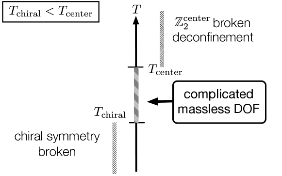
Figure 3: The case $T_{\rm chiral}<T_{\rm center}$. We need massless degrees of freedom (DOF) in the region $T_{\rm chiral}\leq T\leq T_{\rm center}$ to match the ’t Hooft anomaly. The required DOF is very complicated, as explained in the main text.

However, the scenario above has the following flaw. It is reasonable to assume that the color degrees of freedom are confined in the three dimensional effective theory. This is because the three dimensional $\mathrm{SU}(N_{c})$ gauge fields $(A_{C})_{i}~{}(i=1,2,3)$ after the reduction on $S^{1}$ is strongly coupled. So we assume that the color is confined and $\lambda_{L},\lambda_{R}$ are gauge singlets. In Sec. 2 we discussed that the symmetry (sub)group of the theory is (8) and in particular any gauge invariant quantity must be invariant under the element $c^{\prime}_{2}$ defined in (10). Now suppose that the greatest common divisor ${\rm gcd}(N_{c},N_{f})$ between $N_{c}$ and $N_{f}$ is nontrivial,

$${\rm gcd}(N_{c},N_{f})\neq 1.$$ (96)

Define $c_{3}=(c^{\prime}_{2})^{N_{f}/{\rm gcd}(N_{c},N_{f})}$ which is a nontrivial element when ${\rm gcd}(N_{c},N_{f})\neq 1$. Then, regardless of the baryon charges of $\lambda_{L,R}$, these fermions transform nontrivially under $c_{3}$ because they are in the fundamental representation of $\mathrm{SU}(N_{f})_{L,R}$. This is a contradiction. Therefore, if ${\rm gcd}(N_{c},N_{f})\neq 1$, the above scenario is excluded. This is in perfect agreement with the results of Shimizu:2017asf . In that work, a very nontrivial anomaly was found under the condition ${\rm gcd}(N_{c},N_{f})\neq 1$ which cannot be matched by fermions alone. Here we got the same conclusion as in Shimizu:2017asf by a different (but closely related) argument.

If ${\rm gcd}(N_{c},N_{f})=1$, the above argument cannot be directly applied. However, it is unlikely that the order of $T_{\rm chiral}$ and $T_{\rm center}$ changes depending on the precise value of ${\rm gcd}(N_{c},N_{f})$. For example, consider the case $N_{c}=15$. Is it possible that $T_{\rm chiral}<T_{\rm center}$ for $N_{f}=4$ but $T_{\rm chiral}\geq T_{\rm center}$ for $N_{f}=3$ and $N_{f}=5$? We do not see such kind of sensitivity on ${\rm gcd}(N_{c},N_{f})$ in the dynamics of exactly solvable theories such as supersymmetric QCD (see Intriligator:1995au for a review). Therefore, the above scenario is very unlikely even if ${\rm gcd}(N_{c},N_{f})=1$ at least for generic values of $(N_{c},N_{f})$.

There are more reasons to think that the above scenario is unlikely. For generic values of $(N_{f},N_{c})$, the baryon charges of $\lambda_{L,R}$ must be taken to be some peculiar number to satisfy the condition that they are invariant under $c^{\prime}_{2}$. So we must demand that some baryons with complicated baryon charges become massless for the above scenario to be realized.

Moreover, if $N_{c}$ is even, all gauge invariant quantities are bosonic. Then the fermions $\lambda_{L,R}$ cannot exist if they are gauge singlets.

Therefore, we expect that for generic $(N_{c},N_{f})$ the above scenario is very unlikely. It could still happen that for some special $N_{f}$ given by some critical value $N_{f}^{*}(N_{c})$ which is a function of $N_{c}$, the above scenario in terms of the $\lambda_{L,R}$ is realized. For example, in supersymmetric QCD, it happens at $N_{f}^{*}(N_{c})=N_{c}+1$ in which case $T_{\rm chiral}=0$ while the color is still confined. We do not know such a critical value $N_{f}^{*}(N_{c})$ in non-supersymmetric QCD, but notice that there is a difference from the case of supersymmetric QCD, because it is impossible to have fermions if $N_{c}$ is even as mentioned above.

In the usual (non-supersymmetric) QCD, chiral symmetry breaking may happen at least for $N_{f}\leq N_{c}$. (It can of course happen for larger $N_{f}$, but the range $N_{f}\leq N_{c}$ might be safe from the experience of the real world $N_{f}\mathop{}_{\textstyle\sim}^{\textstyle<}N_{c}=3$ as well as the results in supersymmetric QCD.) It is very likely that in this range of color and flavor numbers we have $T_{\rm chiral}\geq T_{\rm center}$.

There may be a way to avoid the above conclusion if we are willing to accept that some gauge degrees of freedom (in the three dimensional sense $(A_{C})_{i=1,2,3}$) are not confined. For example, suppose that there is a $\mathrm{U}(1)$ gauge field in three dimensions, $(A_{\mathrm{U}(1)})_{i}~{}(i=1,2,3)$ which is not confined, and that $\lambda_{L},\lambda_{R}$ have charges $\pm 1$ under this $\mathrm{U}(1)$. Then these fermions are not gauge singlets anymore, and the action of $c^{\prime}_{2}$ can be compensated by $\mathrm{U}(1)$ gauge transformations. It is possible to see that such a scenario is consistent with the anomaly as follows. Suppose that the Wilson line $W_{\rm quark}$ has a VEV of the form

$$W_{\rm quark}=\mathop{\rm diag}\nolimits(-1,+1,\cdots,+1).$$ (97)

Such a configuration is not a potential minimum at high temperature regime, but for the sake of considering just the anomaly, we neglect that issue. The three dimensional $\mathrm{SU}(N_{c})$ gauge group is spontaneously broken to $\mathrm{SU}(N_{c}-1)\times\mathrm{U}(1)$ by the above VEV of $W_{\rm quark}$, and after confinement of $\mathrm{SU}(N_{c}-1)$ we get a $\mathrm{U}(1)$ gauge field. The components of the quarks which are coupled to the eigenvalue $(-1)$ of $W_{\rm quark}$ give massless fermions coupled to the $\mathrm{U}(1)$ and they contribute to the anomaly as is clear from the derivation of the anomaly in Sec. 2. Therefore, as far as the anomaly is concerned, it is possible that we have the fermions $(\lambda_{L},\lambda_{R})$ coupled to a $\mathrm{U}(1)$ gauge field. This (and other more complicated scenarios) remain as a logical possibility, but this is a rather exotic scenario. Moreover, it is not clear whether the $\mathrm{U}(1)$ can really remain deconfined or not, because it is strongly coupled for small $N_{f}$. Therefore, we assume that this does not happen and hence $T_{\rm chiral}\geq T_{\rm center}$ in the following.

Indeed, the inequality $T_{\rm chiral}\geq T_{\rm center}$ was seen Aharony:2006da ; Mandal:2011ws ; Isono:2015uda in a holographic model of QCD Sakai:2004cn . There is a one parameter family of such holographic models, and depending on the parameter we can realize both of the cases $T_{\rm chiral}=T_{\rm center}$ and $T_{\rm chiral}>T_{\rm center}$. The holographic QCD contains several degrees of freedom which were not present in the QCD, and those degrees of freedom may be responsible for the difference.

In fact, it is easy to realize the inequality $T_{\rm chiral}>T_{\rm center}$ without changing the anomaly by considering the following simple toy model. Let us add to the QCD an elementary scalar field $S$ which is an $N_{f}\times N_{f}$ matrix and transforms under $(g_{L},g_{R})\in\mathrm{SU}(N_{f})_{L}\times\mathrm{SU}(N_{f})_{R}$ as $g_{L}Sg_{R}^{\dagger}$. We may introduce a yukawa coupling $\operatorname{tr}_{f}(S^{\dagger}\psi_{L}\psi_{R})$ between the elementary scalar $S$ and the quarks $\psi_{L}$ and $\psi_{R}$. By changing the potential $V(S)$ of the scalar field $S$, we can break the chiral symmetry at an arbitrary scale $\left\langle{S}\right\rangle$. We may take the scale to be much larger than the dynamical scale $\Lambda$ of the gauge theory. In this way we can realize the situation $T_{\rm chiral}>T_{\rm center}$. This is possible since we have two independent scales $\left\langle{S}\right\rangle$ and $\Lambda$. The parameter mentioned above in the holographic QCD might be something like the VEV $\left\langle{S}\right\rangle$ which can be taken independent of $\Lambda$.

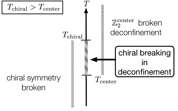
Figure 4: The case $T_{\rm chiral}>T_{\rm center}$. In the range $T_{\rm chiral}>T>T_{\rm center}$, the chiral symmetry is broken even thougth the theory is in deconfinement phase.

However, in the absence of such elementary scalar fields, it may be more natural to have the situation $T_{\rm chiral}=T_{\rm center}$ by the following reason. Suppose contrary that we have $T_{\rm chiral}>T_{\rm center}$ as in Figure 4. Recall that $T_{\rm center}$ can be interpreted as the temperature of confinement/deconfinement phase transition. Then, $T_{\rm chiral}>T_{\rm center}$ means that the chiral symmetry is broken in the deconfinement phase. If we introduce elementary scalar fields $S$ as above, it is easily realized. However, in the absence of such scalars, the chiral symmetry should be broken by quark condensates. Intuitively, the quarks and anti-quarks are not so strongly bounded in the deconfinement phase and it is difficult to imagine that the quark condensation occurs in such a deconfinement phase. Although $T_{\rm chiral}>T_{\rm center}$ is allowed by the anomaly, it is rather exotic. Therefore, the possibility $T_{\rm chiral}=T_{\rm center}$ is more natural in the QCD which contains only the dynamical scale $\Lambda$ as a parameter. The fact that the holographic QCD realizes such a case at least for certain parameter range Aharony:2006da ; Mandal:2011ws ; Isono:2015uda is an evidence for this claim. Therefore we may consider $T_{\rm chiral}=T_{\rm center}$ as the most natural possibility, and denote this temperature as

$$T_{c}:=T_{\rm chiral}=T_{\rm center}.$$ (98)

This is the single critical temperature.

Finally, we need to ask whether the phase transition at $T_{c}$ is first order or second order. If it is second order, the situation is actually not so different from the case of $T_{\rm chiral}<T_{\rm center}$ which we have discussed above. The reason is that at $T=T_{c}$ both of the symmetries ${\mathbb{Z}}_{2}^{\rm center}$ and $\mathrm{SU}(N_{f})_{L}\times\mathrm{SU}(N_{f})_{R}$ are preserved because a second order phase transition is continuous (though not smooth) and these symmetries are unbroken at either $T<T_{c}$ or $T>T_{c}$. Therefore, we need massless fermions like $\lambda_{L}$ and $\lambda_{R}$ which are coupled to a $\mathrm{U}(1)$ gauge field, or more exotic degrees of freedom. Even worse, $T_{\rm chiral}=T_{\rm center}$ seems to be fine-tuning once we accept the appearance of $\lambda_{L,R}$, because we can match the anomaly even if $T_{\rm chiral}<T_{\rm center}$ in that case. There seems to be no particular reason that $T_{\rm chiral}$ and $T_{\rm center}$ coincides. Therefore, we regard a second order transition at $T_{c}$ as unlikely for generic values of $(N_{c},N_{f})$.

By the above arguments, we conclude that the most natural scenario may be a first order phase transition at the single critical temperature (98) as in Figure 5. This is what was discussed in Shimizu:2017asf . Of course, each of the above steps relies on some intuition about strong dynamics, and some exotic possibilities could be realized if such intuition is violated. It would be very interesting to investigate these points further.

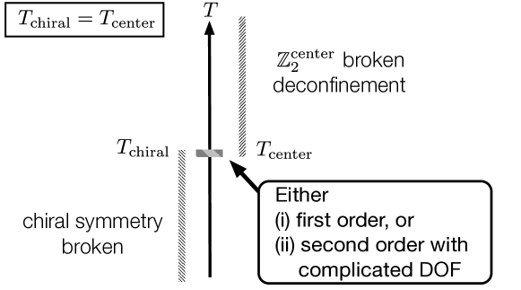
Figure 5: The case $T_{\rm chiral}=T_{\rm center}$. A first order phase transition is natural. If it is second order, some complicated massless DOF must appear at the critical temperature to match the ’t Hooft anomaly.

4.2.2 $\mu_{B}=0$

Let us next move to the case $\mu_{B}=0$. We argued above that a first order phase transition at a single critical temperature $T_{c}$ is the most natural possibility, at least for generic $(N_{c},N_{f})$ with $N_{f}\mathop{}_{\textstyle\sim}^{\textstyle<}N_{c}$. We assume that this is the case. Can this conclusion change if we vary the value of $\mu_{B}$?

We have seen in the previous subsection that the dependence of the free energy on $\mu_{B}$ is given by (75) at high temperatures. From this, we can also see that the entropy (defined formally as $S=-(\partial F)/(\partial T)$) behaves as

$$S\sim N_{c}^{2}+N_{f}N_{c}+\frac{N_{f}}{N_{c}}\mu_{B}^{2}.$$ (99)

The point is that $\mu_{B}$ only changes the entropy by an order of $N_{f}/N_{c}$.

On the other hand, in a first order phase transition, it is natural to think that the entropy changes by an order $N_{c}^{2}$ if $N_{f}\mathop{}_{\textstyle\sim}^{\textstyle<}N_{c}$. For example, in the high and low temperature limits we have $S\sim c_{\rm high}N_{c}^{2}$ for $T\gg\Lambda$ from gluons and $S\sim c_{\rm low}N_{f}^{2}$ for $T\ll\Lambda$ from Goldstone bosons with different numerical coefficients $c_{\rm high}\neq c_{\rm low}$. So let us assume that the entropy changes by an order of $N_{c}^{2}$.

Compared to the change of the entropy $\Delta S\sim N_{c}^{2}$ in the phase transition, the effect of the imaginary chemical potential $(N_{f}/N_{c})\mu_{B}^{2}$ is sub-leading in the large $N$ expansion. This is true even if the flavor number $N_{f}$ is comparable to $N_{c}$, $N_{f}\sim N_{c}$. Therefore, it is natural to think that the imaginary chemical potential does not change the qualitative behavior of what we have found above, at least in the large $N_{c}$ limit.

We conclude that the first order phase transition is the most natural possibility even for the case $\mu_{B}=0$. This argument is more solid for larger values of $N_{c}$. The value of interest in the real world, $N_{c}=3$, is a marginal value because $N_{c}=2$ and $N_{c}\geq 3$ has different qualitative structure (e.g. whether the anti-fundamental representation of $\mathrm{SU}(N_{c})$ is the same as the fundamental representation). The qualitative success of large $N_{c}$ expansion in QCD phenomenology suggests that we should take large $N_{c}$ analysis seriously, as emphasized in Witten:1979kh .

4.2.3 Comparison with pure Yang-Mills at $\theta=\pi$ and $\theta=0$

There is some analogy between QCD at finite temperature with $\mu_{B}=\pi$ and pure Yang-Mills at finite temperature with $\theta=\pi$. In the case of pure Yang-Mills, the relevant symmetries (in three dimensions after compactification on the thermal circle $S^{1}$) are time-reversal symmetry ${\mathsf{T}}$, zero-form center symmetry ${\mathbb{Z}}_{N_{c}}^{\rm center}$, and one-form center symmetry ${\mathbb{Z}}_{N_{c}}^{\rm center(1)}$. There is a mixed anomaly among these three symmetries which severely constrains the nature of thermal phase transition Gaiotto:2017yup . We assume that the one-form center symmetry is always unbroken, and in the following, the zero-form center symmetry is just called the center symmetry. We denote the critical temperatures associated to the symmetries ${\mathsf{T}}$ and ${\mathbb{Z}}_{N_{c}}^{\rm center}$ as $T_{\mathsf{T}}$ and $T_{\rm center}$, respectively. The time-reversal is preserved at high temperature $T>T_{\mathsf{T}}$ and broken at low temperature $T<T_{\mathsf{T}}$. The center symmetry is broken at high temperature $T>T_{\rm center}$ and preserved at low temperature $T<T_{\rm center}$. Therefore, in the analogy with QCD, the time-reversal corresponds to $\mathrm{SU}(N_{f})_{L}\times\mathrm{SU}(N_{f})_{R}$, and ${\mathbb{Z}}_{N_{c}}^{\rm center}$ corresponds to ${\mathbb{Z}}_{2}^{\rm center}$.

For the pure Yang-Mills at $\theta=\pi$, let us repeat the argument we have given above for QCD. First of all, suppose that $T_{\mathsf{T}}<T_{\rm center}$. Then all the symmetries are preserved at $T_{\mathsf{T}}\leq T\leq T_{\rm center}$, and we need complicated degrees of freedom to match the anomaly. In fact, if we assume only the degrees of freedom which are naturally expected from the Yang-Mills, it is not possible to match the anomaly as discussed in detail in Gaiotto:2017yup . Therefore, it is very likely that $T_{\mathsf{T}}\geq T_{\rm center}$.

Next, let us ask whether $T_{\mathsf{T}}>T_{\rm center}$ is natural or not. Recall that $T_{\rm center}$ is the temperature of confinement/deconfinement phase transition. Then, if the inequality $T_{\mathsf{T}}>T_{\rm center}$ is satisfied, that means that the time-reversal is broken in the deconfinement phase in the temperature range $T_{\rm center}<T<T_{\mathsf{T}}$. In pure Yang-Mills theory, one of the natural order parameters for the time-reversal at zero temperature is the parity odd glueball operator $G_{A}=\operatorname{tr}_{c}(F_{\mu\nu}F_{\rho\sigma})\epsilon^{\mu\nu\rho\sigma}$. In fact, in the Euclidean path integral at zero temperature, $\left\langle{G_{A}}\right\rangle\propto-\frac{\partial}{\partial\theta}\log Z=\frac{\partial}{\partial\theta}V(\theta)$ where $Z$ is the partition function and $V(\theta)$ is the vacuum energy as a function of $\theta$. At least in the large $N_{c}$ limit, this potential behaves as $V(\theta)\propto\theta^{2}$ Witten:1979vv ; Witten:1980sp ; Witten:1998uka ; Yonekura:2014oja ; Yamazaki:2017ulc and hence $\left\langle{G_{A}}\right\rangle\neq 0$.

However, there is a subtlety which was not present in QCD. Although $G_{A}$ is the most natural order parameter at zero temperature, the ’t Hooft and dyonic line operators wrapped on the thermal circle $S^{1}$ are also good order parameters at finite temperature Gaiotto:2017yup . To pursue the analogy with the QCD, we neglect this subtle issue and regard $G_{A}$ as the most relevant order parameter. Assuming this, the intuitive picture of the time-reversal breaking is that there is gluon condensation; from a pair of gluon fields $F_{\mu\nu}$ and $F_{\rho\sigma}$, we make the operator corresponding to the bound state of the gluons as $G_{A}=\operatorname{tr}_{c}(F_{\mu\nu}F_{\rho\sigma})\epsilon^{\mu\nu\rho\sigma}$. The time-reversal is broken by the condensation of this bound state. However, if the inequality $T_{\mathsf{T}}>T_{\rm center}$ holds, that implies that we have the condensation of gluons even in the deconfinement phase. This is counter-intuitive. Therefore, we regard this scenario to be unlikely, up to the subtlety discussed above. Then $T_{\mathsf{T}}=T_{\rm center}$ may be more natural and we assume it in the following.

Suppose that the phase transition at $T_{c}:=T_{\mathsf{T}}=T_{\rm center}$ is second order. Then all the symmetries are preserved at $T=T_{c}$ and we need complicated degrees of freedom to match the anomaly. As discussed for the case $T_{\mathsf{T}}<T_{\rm center}$, we regard such complicated degrees of freedom to be unlikely. Therefore, we conclude that a first order phase transition at $T_{c}$ is the most natural possibility.

Finally let us change the value of $\theta$. By the standard large $N_{c}$ counting Witten:1979vv ; Witten:1980sp ; Witten:1998uka , the effect of $\theta$ to the partition function and hence the entropy is at most

$$S\sim N_{c}^{2}+\theta^{2}.$$ (100)

The actual effect is more suppressed, but that is not necessary for our purposes here. The point is that the dependence on $\theta$ is just a sub-leading effect in the large $N_{c}$ expansion. On the other hand, in the first order deconfinement phase transition, it is natural to consider that the entropy changes by the order of $N_{c}^{2}$. Therefore, it seems unlikely that the value of $\theta$ affects the qualitative behavior of the first order phase transition if the large $N_{c}$ expansion is qualitatively good.

From the above considerations, we conclude that a first order phase transition is the most natural possibility even at $\theta=0$, if large $N_{c}$ expansion is qualitatively good. This is what is strongly believed to be the case. For an explicit lattice simulation, see e.g. Panero:2009tv , where first order transitions are seen for $N_{c}\geq 3$. In holographic models, deconfinement phase transitions are always first order because they involve the change of the spacetime topology (see e.g Witten:1998zw ; Aharony:2006da ). Notice that the first order transition for large $N_{c}$ pure Yang-Mills at $\theta=0$ may not follow from the argument of universality. Most naively, in the large $N_{c}$ limit the symmetry ${\mathbb{Z}}_{N_{c}}^{\rm center}$ becomes effectively $\mathrm{U}(1)$, and the Polyakov loop operator $L$ is the order parameter of this symmetry, so the universality class might seem to be that of $\mathrm{O}(2)$ Wilson-Fisher fixed point with the effective Lagrangian of the form ${\cal L}\sim|\partial_{i}L|^{2}-(T-T_{c})|L|^{2}+|L|^{4}$. This is not the case in large $N_{c}$ pure Yang-Mills.

Therefore we have “successfully shown” the first order phase transition of large $N_{c}$ pure Yang-Mills theory from considerations of the anomaly and the large $N$ expansion. Of course, as in the case of the discussions in QCD, each of the steps of the discussions was not rigorous, and in particular there was an additional subtlety in pure Yang-Mills related to the order parameter of the breaking of ${\mathsf{T}}$ as discussed above. But this “success” might give some confidence that the discussions given above for the case of QCD is in the right direction. Obviously more detailed studies from various directions would be desirable.

4.3 Discussion

The real QCD has two well-known small expansion parameters:

• The masses $m_{q}$ of the light quarks $q=u,d,(s)$.

• $1/N_{c}$, where $N_{c}=3$.

At least at zero temperature, they are known to be good expansion parameters. Here, “good” means that arguments based on the expansion about them explain many qualitative (even if not quantitative) properties of QCD dynamics at zero temperature.

In this paper, the large $N_{c}$ expansion has appeared in the discussions of how the thermodynamics depends on the imaginary baryon chemical potential $\mu_{B}$. We mainly discussed the point $\mu_{B}=\pi$ to make the concept of confinement well-defined, but the effect of $\mu_{B}$ is highly suppressed in the large $N_{c}$ expansion. Also, we focused our attention to $m_{q}=0$.

In the applications of QCD phase transition to early cosmology, we are interested in the physical quark masses $m_{q}\neq 0$ and zero imaginary chemical potential $\mu_{B}=0$. This physical situation is the same at the leading order of expansion to the situation we have studied in this paper, $m_{q}=0$ and $\mu_{B}=\pi$. The difference appears only at sub-leading orders in the expansion. The small parameter $m_{q}$ explicitly breaks the symmetry $\mathrm{SU}(N_{f})_{L}\times\mathrm{SU}(N_{f})_{R}$, and the small parameter $(\pi-\mu_{B})/N_{c}$ explicitly breaks the symmetry ${\mathbb{Z}}^{\rm center}_{2}$. Now we can distinguish two cases of phase transition: first order or second order.

• If the phase transition is second order, then at the critical temperature, we have gapless degrees of freedom at $(m_{q},\mu_{B})=(0,\pi)$ which are associated to the symmetries $\mathrm{SU}(N_{f})_{L}\times\mathrm{SU}(N_{f})_{R}$ and ${\mathbb{Z}}^{\rm center}_{2}$. These gapless degrees of freedom get masses by small explicit-breaking parameters $m_{q}$ or $(\pi-\mu_{B})/N_{c}$, and the phase transition becomes cross-over.

• If the phase transition is first order at $(m_{q},\mu_{B})=(0,\pi)$, the order of the phase transition may not change as far as the parameters $m_{q}$ and $1/N_{c}$ are good small expansion parameters.

The ’t Hooft anomaly discussed in this paper constrains the nature of phase transition at $(m_{q},\mu_{B})=(0,\pi)$. There are still many logical possibilities allowed by the anomaly, some of which are shown in Figures 3, 4, and 5. Based on some reasonable intuition about strong dynamics, we have argued that a first order phase transition in Figure 5 may be the most natural scenario. If so, the phase transition at the physical point $m_{q}\neq 0$ and $\mu_{B}=0$ may also be first order if $m_{q}$ and $1/N_{c}$ are good expansion parameters. In other words, if the QCD phase transition at the physical point is cross-over, some of the assumptions about QCD which are reasonable at zero temperature (e.g. expansion in terms of $m_{q}$ and $1/N_{c}$) must be violated at finite temperatures. It is an important problem to settle this issue. For the approximate concepts of chiral symmetry and confinement/deconfinement to be useful in QCD, the parameters $m_{q}$ and $1/N_{c}$ must be regarded as small.

- (1) Y. Aoki, G. Endrodi, Z. Fodor, S. D. Katz, and K. K. Szabo, The Order of the quantum chromodynamics transition predicted by the standard model of particle physics, Nature 443 (2006) 675–678, [hep-lat/0611014].
- (2) T. Bhattacharya et al., QCD Phase Transition with Chiral Quarks and Physical Quark Masses, Phys. Rev. Lett. 113 (2014), no. 8 082001, [arXiv:1402.5175].
- (3) F. Pisarski, Robert D. and Wilczek, Remarks on the Chiral Phase Transition in Chromodynamics, Phys. Rev. D29 (1984) 338–341.
- (4) S. Aoki, H. Fukaya, and Y. Taniguchi, Chiral symmetry restoration, eigenvalue density of Dirac operator and axial U(1) anomaly at finite temperature, Phys. Rev. D86 (2012) 114512, [arXiv:1209.2061].
- (5) JLQCD Collaboration, H. Fukaya, Can axial U(1) anomaly disappear at high temperature?, EPJ Web Conf. 175 (2018) 01012, [arXiv:1712.05536].
- (6) TWQCD Collaboration, T.-W. Chiu, W.-P. Chen, Y.-C. Chen, H.-Y. Chou, and T.-H. Hsieh, Chiral symmetry and axial U(1) symmetry in finite temperature QCD with domain-wall fermion, PoS LATTICE2013 (2014) 165, [arXiv:1311.6220].
- (7) Y. Nakayama and T. Ohtsuki, Bootstrapping phase transitions in QCD and frustrated spin systems, Phys. Rev. D91 (2015), no. 2 021901, [arXiv:1407.6195].
- (8) K. Fukushima and T. Hatsuda, The phase diagram of dense QCD, Rept. Prog. Phys. 74 (2011) 014001, [arXiv:1005.4814].
- (9) H.-T. Ding, Lattice QCD at nonzero temperature and density, PoS LATTICE2016 (2017) 022, [arXiv:1702.00151].
- (10) Y. Aoki, Finite temperature QCD: phase transition, topology, and axion, . available (in the mixture of Japanese and English) at http://www2.yukawa.kyoto-u.ac.jp/ ppp.ws/PPP2018/slides/aoki.pdf.
- (11) D. Gaiotto, A. Kapustin, Z. Komargodski, and N. Seiberg, Theta, Time Reversal, and Temperature, arXiv:1703.00501.
- (12) H. Itoyama and A. H. Mueller, The Axial Anomaly at Finite Temperature, Nucl. Phys. B218 (1983) 349–365.
- (13) S. Weinberg, The quantum theory of fields. Vol. 2: Modern applications. Cambridge University Press, 2013.
- (14) Y. Tachikawa and K. Yonekura, Gauge interactions and topological phases of matter, PTEP 2016 (2016), no. 9 093B07, [arXiv:1604.06184].
- (15) M. Yamazaki and K. Yonekura, From 4d Yang-Mills to 2d model: IR problem and confinement at weak coupling, JHEP 07 (2017) 088, [arXiv:1704.05852].
- (16) Y. Tanizaki and Y. Kikuchi, Vacuum structure of bifundamental gauge theories at finite topological angles, arXiv:1705.01949.
- (17) Z. Komargodski, T. Sulejmanpasic, and M. Unsal, Walls, anomalies, and deconfinement in quantum antiferromagnets, Phys. Rev. B97 (2018), no. 5 054418, [arXiv:1706.05731].
- (18) H. Shimizu and K. Yonekura, Anomaly constraints on deconfinement and chiral phase transition, Phys. Rev. D97 (2018), no. 10 105011, [arXiv:1706.06104].
- (19) Y. Kikuchi and Y. Tanizaki, Global inconsistency, ’t Hooft anomaly, and level crossing in quantum mechanics, PTEP 2017 (2017) 113B05, [arXiv:1708.01962].
- (20) D. Gaiotto, Z. Komargodski, and N. Seiberg, Time-reversal breaking in QCD4, walls, and dualities in 2 + 1 dimensions, JHEP 01 (2018) 110, [arXiv:1708.06806].
- (21) E. Poppitz and M. E. Shalchian T., String tensions in deformed Yang-Mills theory, JHEP 01 (2018) 029, [arXiv:1708.08821].
- (22) P. Di Vecchia, G. Rossi, G. Veneziano, and S. Yankielowicz, Spontaneous breaking in QCD and the axion potential: an effective Lagrangian approach, JHEP 12 (2017) 104, [arXiv:1709.00731].
- (23) R. Kitano, T. Suyama, and N. Yamada, in gauge theories, JHEP 09 (2017) 137, [arXiv:1709.04225].
- (24) Y. Tanizaki, T. Misumi, and N. Sakai, Circle compactification and ?t Hooft anomaly, JHEP 12 (2017) 056, [arXiv:1710.08923].
- (25) M. Yamazaki, Relating ’t Hooft Anomalies of 4d Pure Yang-Mills and 2d Model, arXiv:1711.04360.
- (26) Y. Tanizaki, Y. Kikuchi, T. Misumi, and N. Sakai, Anomaly matching for the phase diagram of massless -QCD, Phys. Rev. D97 (2018), no. 5 054012, [arXiv:1711.10487].
- (27) A. Cherman and M. Unsal, Critical behavior of gauge theories and Coulomb gases in three and four dimensions, arXiv:1711.10567.
- (28) M. Guo, P. Putrov, and J. Wang, Time reversal, SU(N) Yang?Mills and cobordisms: Interacting topological superconductors/insulators and quantum spin liquids in 3+1D, Annals Phys. 394 (2018) 244–293, [arXiv:1711.11587].
- (29) P. Draper, Domain Walls and the Anomaly in Softly Broken Supersymmetric QCD, Phys. Rev. D97 (2018), no. 8 085003, [arXiv:1801.05477].
- (30) N. Seiberg, Y. Tachikawa, and K. Yonekura, Anomalies of Duality Groups and Extended Conformal Manifolds, PTEP 2018 (2018), no. 7 073B04, [arXiv:1803.07366].
- (31) M. Shifman, Supersymmetric tools in Yang?Mills theories at strong coupling: The beginning of a long journey, Int. J. Mod. Phys. A33 (2018), no. 12 1830009, [arXiv:1804.01191].
- (32) A. Ritz and A. Shukla, Domain wall moduli in softly-broken SQCD at , Phys. Rev. D97 (2018), no. 10 105015, [arXiv:1804.01978].
- (33) K. Aitken, A. Cherman, and M. Unsal, Dihedral symmetry in Yang-Mills theory, arXiv:1804.05845.
- (34) K. Aitken, A. Cherman, and M. Unsal, Vacuum structure of Yang-Mills theory as a function of , arXiv:1804.06848.
- (35) M. M. Anber and E. Poppitz, On two-flavor QCD(adj), arXiv:1805.12290.
- (36) R. Argurio, M. Bertolini, F. Bigazzi, A. L. Cotrone, and P. Niro, QCD domain walls, Chern-Simons theories and holography, arXiv:1806.08292.
- (37) C. Córdova and T. T. Dumitrescu, Candidate Phases for SU(2) Adjoint QCD4 with Two Flavors from Supersymmetric Yang-Mills Theory, arXiv:1806.09592.
- (38) M. M. Anber and E. Poppitz, Anomaly matching, (axial) Schwinger models, and high-T super Yang-Mills domain walls, arXiv:1807.00093.
- (39) Y. Tanizaki, Anomaly constraint on massless QCD and the role of Skyrmions in chiral symmetry breaking, arXiv:1807.07666.
- (40) Z. Bi and T. Senthil, An Adventure in Topological Phase Transitions in 3+1-D: Non-abelian Deconfined Quantum Criticalities and a Possible Duality, arXiv:1808.07465.
- (41) S. Yamaguchi, ?t Hooft anomaly matching condition and chiral symmetry breaking without bilinear condensate, JHEP 01 (2019) 014, [arXiv:1811.09390].
- (42) M. M. Anber and E. Poppitz, Domain walls in high- super Yang-Mills theory and QCD(adj), arXiv:1811.10642.
- (43) V. Bashmakov, F. Benini, S. Benvenuti, and M. Bertolini, Living on the walls of super-QCD, arXiv:1812.04645.
- (44) P.-S. Hsin, H. T. Lam, and N. Seiberg, Comments on One-Form Global Symmetries and Their Gauging in 3d and 4d, arXiv:1812.04716.
- (45) Z. Wan and J. Wang, New Higher Anomalies, SU(N) Yang-Mills Gauge Theory and Sigma Model, arXiv:1812.11968.
- (46) M. G. Alford, A. Kapustin, and F. Wilczek, Imaginary chemical potential and finite fermion density on the lattice, Phys. Rev. D59 (1999) 054502, [hep-lat/9807039].
- (47) M.-P. Lombardo, Finite density (might well be easier) at finite temperature, Nucl. Phys. Proc. Suppl. 83 (2000) 375–377, [hep-lat/9908006].
- (48) P. de Forcrand and O. Philipsen, The QCD phase diagram for small densities from imaginary chemical potential, Nucl. Phys. B642 (2002) 290–306, [hep-lat/0205016].
- (49) P. de Forcrand and O. Philipsen, The QCD phase diagram for three degenerate flavors and small baryon density, Nucl. Phys. B673 (2003) 170–186, [hep-lat/0307020].
- (50) P. de Forcrand and O. Philipsen, The Chiral critical line of N(f) = 2+1 QCD at zero and non-zero baryon density, JHEP 01 (2007) 077, [hep-lat/0607017].
- (51) P. de Forcrand and O. Philipsen, The Chiral critical point of N(f) = 3 QCD at finite density to the order (mu/T)**4, JHEP 11 (2008) 012, [arXiv:0808.1096].
- (52) M. D’Elia and M.-P. Lombardo, Finite density QCD via imaginary chemical potential, Phys. Rev. D67 (2003) 014505, [hep-lat/0209146].
- (53) M. D’Elia and M. P. Lombardo, QCD thermodynamics from an imaginary mu(B): Results on the four flavor lattice model, Phys. Rev. D70 (2004) 074509, [hep-lat/0406012].
- (54) V. Azcoiti, G. Di Carlo, A. Galante, and V. Laliena, Phase diagram of QCD with four quark flavors at finite temperature and baryon density, Nucl. Phys. B723 (2005) 77–90, [hep-lat/0503010].
- (55) H.-S. Chen and X.-Q. Luo, Phase diagram of QCD at finite temperature and chemical potential from lattice simulations with dynamical Wilson quarks, Phys. Rev. D72 (2005) 034504, [hep-lat/0411023].
- (56) F. Karbstein and M. Thies, How to get from imaginary to real chemical potential, Phys. Rev. D75 (2007) 025003, [hep-th/0610243].
- (57) P. Cea, L. Cosmai, M. D’Elia, and A. Papa, Analytic continuation from imaginary to real chemical potential in two-color QCD, JHEP 02 (2007) 066, [hep-lat/0612018].
- (58) P. Cea, L. Cosmai, M. D’Elia, and A. Papa, The Critical line from imaginary to real baryonic chemical potentials in two-color QCD, Phys. Rev. D77 (2008) 051501, [arXiv:0712.3755].
- (59) P. Cea, L. Cosmai, M. D’Elia, and A. Papa, The phase diagram of QCD with four degenerate quarks, Phys. Rev. D81 (2010) 094502, [arXiv:1004.0184].
- (60) L.-K. Wu, X.-Q. Luo, and H.-S. Chen, Phase structure of lattice QCD with two flavors of Wilson quarks at finite temperature and chemical potential, Phys. Rev. D76 (2007) 034505, [hep-lat/0611035].
- (61) K. Nagata and A. Nakamura, Imaginary Chemical Potential Approach for the Pseudo-Critical Line in the QCD Phase Diagram with Clover-Improved Wilson Fermions, Phys. Rev. D83 (2011) 114507, [arXiv:1104.2142].
- (62) P. Giudice and A. Papa, Real and imaginary chemical potential in two color QCD, Phys. Rev. D69 (2004) 094509, [hep-lat/0401024].
- (63) M. D’Elia, F. Di Renzo, and M. P. Lombardo, The Strongly interacting quark gluon plasma, and the critical behaviour of QCD at imaginary mu, Phys. Rev. D76 (2007) 114509, [arXiv:0705.3814].
- (64) P. Cea, L. Cosmai, M. D’Elia, C. Manneschi, and A. Papa, Analytic continuation of the critical line: Suggestions for QCD, Phys. Rev. D80 (2009) 034501, [arXiv:0905.1292].
- (65) A. Alexandru and A. Li, QCD at imaginary chemical potential with Wilson fermions, PoS LATTICE2013 (2014) 208, [arXiv:1312.1201].
- (66) P. Cea, L. Cosmai, M. D’Elia, A. Papa, and F. Sanfilippo, The critical line of two-flavor QCD at finite isospin or baryon densities from imaginary chemical potentials, Phys. Rev. D85 (2012) 094512, [arXiv:1202.5700].
- (67) S. Conradi and M. D’Elia, Imaginary chemical potentials and the phase of the fermionic determinant, Phys. Rev. D76 (2007) 074501, [arXiv:0707.1987].
- (68) M. D’Elia and F. Sanfilippo, Thermodynamics of two flavor QCD from imaginary chemical potentials, Phys. Rev. D80 (2009) 014502, [arXiv:0904.1400].
- (69) T. Takaishi, P. de Forcrand, and A. Nakamura, Equation of State at Finite Density from Imaginary Chemical Potential, PoS LAT2009 (2009) 198, [arXiv:1002.0890].
- (70) P. Cea, L. Cosmai, and A. Papa, Critical line of 2+1 flavor QCD, Phys. Rev. D89 (2014), no. 7 074512, [arXiv:1403.0821].
- (71) P. Cea, L. Cosmai, and A. Papa, Critical line of 2+1 flavor QCD: Toward the continuum limit, Phys. Rev. D93 (2016), no. 1 014507, [arXiv:1508.07599].
- (72) C. Bonati, P. de Forcrand, M. D’Elia, O. Philipsen, and F. Sanfilippo, Chiral phase transition in two-flavor QCD from an imaginary chemical potential, Phys. Rev. D90 (2014), no. 7 074030, [arXiv:1408.5086].
- (73) C. Bonati, M. D’Elia, M. Mariti, M. Mesiti, F. Negro, and F. Sanfilippo, Curvature of the chiral pseudocritical line in QCD, Phys. Rev. D90 (2014), no. 11 114025, [arXiv:1410.5758].
- (74) C. Bonati, M. D’Elia, M. Mariti, M. Mesiti, F. Negro, and F. Sanfilippo, Curvature of the chiral pseudocritical line in QCD: Continuum extrapolated results, Phys. Rev. D92 (2015), no. 5 054503, [arXiv:1507.03571].
- (75) R. Bellwied, S. Borsanyi, Z. Fodor, J. Gunther, S. D. Katz, C. Ratti, and K. K. Szabo, The QCD phase diagram from analytic continuation, Phys. Lett. B751 (2015) 559–564, [arXiv:1507.07510].
- (76) J. N. Guenther, R. Bellwied, S. Borsanyi, Z. Fodor, S. D. Katz, A. Pasztor, C. Ratti, and K. K. Szabo, The QCD equation of state at finite density from analytical continuation, Nucl. Phys. A967 (2017) 720–723, [arXiv:1607.02493].
- (77) M. D’Elia, G. Gagliardi, and F. Sanfilippo, Higher order quark number fluctuations via imaginary chemical potentials in QCD, Phys. Rev. D95 (2017), no. 9 094503, [arXiv:1611.08285].
- (78) V. G. Bornyakov, D. L. Boyda, V. A. Goy, H. Iida, A. V. Molochkov, A. Nakamura, A. A. Nikolaev, V. I. Zakharov, and M. Wakayama, Lattice QCD at finite baryon density using analytic continuation, in 6th International Conference on New Frontiers in Physics (ICNFP 2017) Kolymbari, Crete, Greece, August 17-26, 2017, 2017. arXiv:1712.02830.
- (79) M. Andreoli, C. Bonati, M. D’Elia, M. Mesiti, F. Negro, A. Rucci, and F. Sanfilippo, Gauge-invariant screening masses and static quark free energies in QCD at nonzero baryon density, Phys. Rev. D97 (2018), no. 5 054515, [arXiv:1712.09996].
- (80) J. Greensite and K. Langfeld, Finding the effective Polyakov line action for SU(3) gauge theories at finite chemical potential, Phys. Rev. D90 (2014), no. 1 014507, [arXiv:1403.5844].
- (81) J. Greensite, Comparison of complex Langevin and mean field methods applied to effective Polyakov line models, Phys. Rev. D90 (2014), no. 11 114507, [arXiv:1406.4558].
- (82) J. Takahashi, H. Kouno, and M. Yahiro, Quark number densities at imaginary chemical potential in lattice QCD with Wilson fermions and its model analyses, Phys. Rev. D91 (2015), no. 1 014501, [arXiv:1410.7518].
- (83) J. Takahashi, J. Sugano, M. Ishii, H. Kouno, and M. Yahiro, Quark number density at imaginary chemical potential and its extrapolation to large real chemical potential by the effective model, PoS LATTICE2014 (2015) 187, [arXiv:1410.8279].
- (84) J. Greensite and R. Hollwieser, Finite-density transition line for QCD with 695 MeV dynamical fermions, Phys. Rev. D97 (2018), no. 11 114504, [arXiv:1708.08031].
- (85) M. D’Elia and F. Sanfilippo, The Order of the Roberge-Weiss endpoint (finite size transition) in QCD, Phys. Rev. D80 (2009) 111501, [arXiv:0909.0254].
- (86) P. de Forcrand and O. Philipsen, Constraining the QCD phase diagram by tricritical lines at imaginary chemical potential, Phys. Rev. Lett. 105 (2010) 152001, [arXiv:1004.3144].
- (87) C. Bonati, G. Cossu, M. D’Elia, and F. Sanfilippo, The Roberge-Weiss endpoint in = 2 QCD, Phys. Rev. D83 (2011) 054505, [arXiv:1011.4515].
- (88) O. Philipsen and C. Pinke, Nature of the Roberge-Weiss transition in QCD with Wilson fermions, Phys. Rev. D89 (2014), no. 9 094504, [arXiv:1402.0838].
- (89) L.-K. Wu and X.-F. Meng, Nature of the Roberge-Weiss transition end points in two-flavor lattice QCD with Wilson quarks, Phys. Rev. D87 (2013), no. 9 094508, [arXiv:1303.0336].
- (90) L.-K. Wu and X.-F. Meng, Nature of Roberge-Weiss transition endpoints for heavy quarks in 2 lattice QCD with Wilson fermions, Phys. Rev. D90 (2014), no. 9 094506, [arXiv:1405.2425].
- (91) K. Nagata, K. Kashiwa, A. Nakamura, and S. M. Nishigaki, Lee-Yang zero distribution of high temperature QCD and the Roberge-Weiss phase transition, Phys. Rev. D91 (2015), no. 9 094507, [arXiv:1410.0783].
- (92) K. Kashiwa and A. Ohnishi, Quark number holonomy and confinement-deconfinement transition, Phys. Rev. D93 (2016), no. 11 116002, [arXiv:1602.06037].
- (93) K. Kashiwa and A. Ohnishi, Topological feature and phase structure of QCD at complex chemical potential, Phys. Lett. B750 (2015) 282–286, [arXiv:1505.06799].
- (94) C. Bonati, M. D’Elia, M. Mariti, M. Mesiti, F. Negro, and F. Sanfilippo, Roberge-Weiss endpoint at the physical point of QCD, Phys. Rev. D93 (2016), no. 7 074504, [arXiv:1602.01426].
- (95) T. Makiyama, Y. Sakai, T. Saito, M. Ishii, J. Takahashi, K. Kashiwa, H. Kouno, A. Nakamura, and M. Yahiro, Phase structure of two-color QCD at real and imaginary chemical potentials; lattice simulations and model analyses, Phys. Rev. D93 (2016), no. 1 014505, [arXiv:1502.06191].
- (96) C. Pinke and O. Philipsen, The chiral phase transition from imaginary chemical potential with Wilson Fermions, PoS LATTICE2015 (2016) 149, [arXiv:1508.07725].
- (97) C. Czaban, F. Cuteri, O. Philipsen, C. Pinke, and A. Sciarra, Roberge-Weiss transition in QCD with Wilson fermions and , Phys. Rev. D93 (2016), no. 5 054507, [arXiv:1512.07180].
- (98) C. Bonati, E. Calore, M. D’Elia, M. Mesiti, F. Negro, F. Sanfilippo, S. F. Schifano, G. Silvi, and R. Tripiccione, Roberge-Weiss endpoint and chiral symmetry restoration in QCD, arXiv:1807.02106.
- (99) H. Kouno, Y. Sakai, K. Kashiwa, and M. Yahiro, Roberge-Weiss phase transition and its endpoint, J. Phys. G36 (2009) 115010, [arXiv:0904.0925].
- (100) Y. Sakai, K. Kashiwa, H. Kouno, M. Matsuzaki, and M. Yahiro, Determination of QCD phase diagram from the imaginary chemical potential region, Phys. Rev. D79 (2009) 096001, [arXiv:0902.0487].
- (101) T. Sasaki, Y. Sakai, H. Kouno, and M. Yahiro, Quark-mass dependence of the three-flavor QCD phase diagram at zero and imaginary chemical potential: Model prediction, Phys. Rev. D84 (2011) 091901, [arXiv:1105.3959].
- (102) H. Kouno, M. Kishikawa, T. Sasaki, Y. Sakai, and M. Yahiro, Spontaneous parity and charge-conjugation violations at real isospin and imaginary baryon chemical potentials, Phys. Rev. D85 (2012) 016001, [arXiv:1110.5187].
- (103) G. Aarts, S. P. Kumar, and J. Rafferty, Holographic Roberge-Weiss Transitions, JHEP 07 (2010) 056, [arXiv:1005.2947].
- (104) J. Rafferty, Holographic Roberge Weiss Transitions II - Defect Theories and the Sakai Sugimoto Model, JHEP 09 (2011) 087, [arXiv:1103.2315].
- (105) K. Morita, V. Skokov, B. Friman, and K. Redlich, Probing deconfinement in a chiral effective model with Polyakov loop at imaginary chemical potential, Phys. Rev. D84 (2011) 076009, [arXiv:1107.2273].
- (106) K. Kashiwa, T. Hell, and W. Weise, Nonlocal Polyakov-Nambu-Jona-Lasinio model and imaginary chemical potential, Phys. Rev. D84 (2011) 056010, [arXiv:1106.5025].
- (107) V. Pagura, D. Gomez Dumm, and N. N. Scoccola, Deconfinement and chiral restoration in nonlocal PNJL models at zero and imaginary chemical potential, Phys. Lett. B707 (2012) 76–82, [arXiv:1105.1739].
- (108) D. Scheffler, M. Buballa, and J. Wambach, PNJL Model Analysis of the Roberge-Weiss Transition Endpoint at Imaginary Chemical Potential, Acta Phys. Polon. Supp. 5 (2012) 971–976, [arXiv:1111.3839].
- (109) K. Kashiwa and R. D. Pisarski, Roberge-Weiss transition and ’t Hooft loops, Phys. Rev. D87 (2013), no. 9 096009, [arXiv:1301.5344].
- (110) K. Kashiwa, T. Sasaki, H. Kouno, and M. Yahiro, Two-color QCD at imaginary chemical potential and its impact on real chemical potential, Phys. Rev. D87 (2013), no. 1 016015, [arXiv:1208.2283].
- (111) E. G. Filothodoros, A. C. Petkou, and N. D. Vlachos, fermion-boson map with imaginary chemical potential, Phys. Rev. D95 (2017), no. 6 065029, [arXiv:1608.07795].
- (112) E. G. Filothodoros, A. C. Petkou, and N. D. Vlachos, The fermion-boson map for large , Nucl. Phys. B941 (2019) 195–224, [arXiv:1803.05950].
- (113) A. Roberge and N. Weiss, Gauge Theories With Imaginary Chemical Potential and the Phases of QCD, Nucl. Phys. B275 (1986) 734–745.
- (114) H. Kouno, Y. Sakai, T. Makiyama, K. Tokunaga, T. Sasaki, and M. Yahiro, Quark-gluon thermodynamics with the Z(N(c)) symmetry, J. Phys. G39 (2012) 085010.
- (115) Y. Sakai, H. Kouno, T. Sasaki, and M. Yahiro, The quarkyonic phase and the Z symmetry, Phys. Lett. B718 (2012) 130–135, [arXiv:1204.0228].
- (116) H. Kouno, T. Makiyama, T. Sasaki, Y. Sakai, and M. Yahiro, Confinement and symmetry in three-flavor QCD, J. Phys. G40 (2013) 095003, [arXiv:1301.4013].
- (117) H. Kouno, T. Misumi, K. Kashiwa, T. Makiyama, T. Sasaki, and M. Yahiro, Differences and similarities between fundamental and adjoint matters in SU(N) gauge theories, Phys. Rev. D88 (2013), no. 1 016002, [arXiv:1304.3274].
- (118) E. Poppitz and T. Sulejmanpasic, (S)QCD on : Screening of Polyakov loop by fundamental quarks and the demise of semi-classics, JHEP 09 (2013) 128, [arXiv:1307.1317].
- (119) T. Iritani, E. Itou, and T. Misumi, Lattice study on QCD-like theory with exact center symmetry, JHEP 11 (2015) 159, [arXiv:1508.07132].
- (120) H. Kouno, K. Kashiwa, J. Takahashi, T. Misumi, and M. Yahiro, Understanding QCD at high density from a Z3-symmetric QCD-like theory, Phys. Rev. D93 (2016), no. 5 056009, [arXiv:1504.07585].
- (121) T. Hirakida, H. Kouno, J. Takahashi, and M. Yahiro, Interplay between sign problem and symmetry in three-dimensional Potts models, Phys. Rev. D94 (2016), no. 1 014011, [arXiv:1604.02977].
- (122) T. Hirakida, J. Sugano, H. Kouno, J. Takahashi, and M. Yahiro, Sign problem in -symmetric effective Polyakov-line model, Phys. Rev. D96 (2017), no. 7 074031, [arXiv:1705.00665].
- (123) A. Cherman, S. Sen, M. Unsal, M. L. Wagman, and L. G. Yaffe, Order parameters and color-flavor center symmetry in QCD, arXiv:1706.05385.
- (124) A. N. Redlich, Parity Violation and Gauge Noninvariance of the Effective Gauge Field Action in Three-Dimensions, Phys. Rev. D29 (1984) 2366–2374. [,2366(1983)].
- (125) A. J. Niemi and G. W. Semenoff, Axial Anomaly Induced Fermion Fractionization and Effective Gauge Theory Actions in Odd Dimensional Space-Times, Phys. Rev. Lett. 51 (1983) 2077.
- (126) L. Alvarez-Gaume, S. Della Pietra, and G. W. Moore, Anomalies and Odd Dimensions, Annals Phys. 163 (1985) 288.
- (127) E. Witten, The ”Parity” Anomaly On An Unorientable Manifold, Phys. Rev. B94 (2016), no. 19 195150, [arXiv:1605.02391].
- (128) E. Witten, Global Aspects of Current Algebra, Nucl. Phys. B223 (1983) 422–432.
- (129) E. Witten, Current Algebra, Baryons, and Quark Confinement, Nucl. Phys. B223 (1983) 433–444.
- (130) M. F. Atiyah, V. K. Patodi, and I. M. Singer, Spectral asymmetry and Riemannian Geometry 1, Math. Proc. Cambridge Phil. Soc. 77 (1975) 43.
- (131) H. Fukaya, T. Onogi, and S. Yamaguchi, Atiyah-Patodi-Singer index from the domain-wall fermion Dirac operator, Phys. Rev. D96 (2017), no. 12 125004, [arXiv:1710.03379].
- (132) M. Bando, T. Kugo, S. Uehara, K. Yamawaki, and T. Yanagida, Is rho Meson a Dynamical Gauge Boson of Hidden Local Symmetry?, Phys. Rev. Lett. 54 (1985) 1215.
- (133) D. S. Freed and M. J. Hopkins, Reflection positivity and invertible topological phases, arXiv:1604.06527.
- (134) K. Yonekura, On the cobordism classification of symmetry protected topological phases, arXiv:1803.10796.
- (135) E. Witten, Fermion Path Integrals And Topological Phases, Rev. Mod. Phys. 88 (2016), no. 3 035001, [arXiv:1508.04715].
- (136) K. Yonekura, Dai-Freed theorem and topological phases of matter, JHEP 09 (2016) 022, [arXiv:1607.01873].
- (137) Z. Komargodski, A. Sharon, R. Thorngren, and X. Zhou, Comments on Abelian Higgs Models and Persistent Order, arXiv:1705.04786.
- (138) E. Witten, Baryons in the 1/n Expansion, Nucl. Phys. B160 (1979) 57–115.
- (139) M. Hanada, G. Ishiki, and H. Watanabe, Partial Deconfinement, arXiv:1812.05494.
- (140) N. Seiberg and E. Witten, Gapped Boundary Phases of Topological Insulators via Weak Coupling, PTEP 2016 (2016), no. 12 12C101, [arXiv:1602.04251].
- (141) Y. Tachikawa and K. Yonekura, On time-reversal anomaly of 2+1d topological phases, PTEP 2017 (2017), no. 3 033B04, [arXiv:1610.07010].
- (142) Y. Tachikawa and K. Yonekura, More on time-reversal anomaly of 2+1d topological phases, Phys. Rev. Lett. 119 (2017), no. 11 111603, [arXiv:1611.01601].
- (143) J. Wang, X.-G. Wen, and E. Witten, Symmetric Gapped Interfaces of SPT and SET States: Systematic Constructions, arXiv:1705.06728.
- (144) I. García-Etxebarria, H. Hayashi, K. Ohmori, Y. Tachikawa, and K. Yonekura, 8d gauge anomalies and the topological Green-Schwarz mechanism, JHEP 11 (2017) 177, [arXiv:1710.04218].
- (145) Y. Tachikawa, On gauging finite subgroups, arXiv:1712.09542.
- (146) J. Wang et al., Tunneling Topological Vacua via Extended Operators: (Spin-)TQFT Spectra and Boundary Deconfinement in Various Dimensions, PTEP 2018 (2018), no. 5 053A01, [arXiv:1801.05416].
- (147) Y. Lee and Y. Tachikawa, A study of time reversal symmetry of abelian anyons, JHEP 07 (2018) 090, [arXiv:1805.02738].
- (148) C.-T. Hsieh, Discrete gauge anomalies revisited, arXiv:1808.02881.
- (149) K. A. Intriligator and N. Seiberg, Lectures on supersymmetric gauge theories and electric-magnetic duality, Nucl. Phys. Proc. Suppl. 45BC (1996) 1–28, [hep-th/9509066]. [,157(1995)].
- (150) V. Borokhov, A. Kapustin, and X.-k. Wu, Topological disorder operators in three-dimensional conformal field theory, JHEP 11 (2002) 049, [hep-th/0206054].
- (151) S. S. Pufu, Anomalous dimensions of monopole operators in three-dimensional quantum electrodynamics, Phys. Rev. D89 (2014), no. 6 065016, [arXiv:1303.6125].
- (152) O. Aharony, J. Sonnenschein, and S. Yankielowicz, A Holographic model of deconfinement and chiral symmetry restoration, Annals Phys. 322 (2007) 1420–1443, [hep-th/0604161].
- (153) G. Mandal and T. Morita, Gregory-Laflamme as the confinement/deconfinement transition in holographic QCD, JHEP 09 (2011) 073, [arXiv:1107.4048].
- (154) H. Isono, G. Mandal, and T. Morita, Thermodynamics of QCD from Sakai-Sugimoto Model, JHEP 12 (2015) 006, [arXiv:1507.08949].
- (155) T. Sakai and S. Sugimoto, Low energy hadron physics in holographic QCD, Prog. Theor. Phys. 113 (2005) 843–882, [hep-th/0412141].
- (156) E. Witten, Anti-de Sitter space, thermal phase transition, and confinement in gauge theories, Adv. Theor. Math. Phys. 2 (1998) 505–532, [hep-th/9803131]. [,89(1998)].
- (157) E. Witten, Current Algebra Theorems for the U(1) Goldstone Boson, Nucl. Phys. B156 (1979) 269–283.
- (158) E. Witten, Large N Chiral Dynamics, Annals Phys. 128 (1980) 363.
- (159) E. Witten, Theta dependence in the large N limit of four-dimensional gauge theories, Phys. Rev. Lett. 81 (1998) 2862–2865, [hep-th/9807109].
- (160) K. Yonekura, Notes on natural inflation, JCAP 1410 (2014), no. 10 054, [arXiv:1405.0734].
- (161) M. Panero, Thermodynamics of the QCD plasma and the large-N limit, Phys. Rev. Lett. 103 (2009) 232001, [arXiv:0907.3719].