Explicit Polar Codes with
Small Scaling Exponent

Abstract

Polar coding gives rise to the first explicit family of codes that provably achieve capacity for a wide range of channels with efficient encoding and decoding. But how fast can polar coding approach capacity as a function of the code length? In finite-length analysis, the scaling between code length and the gap to capacity is usually measured in terms of the scaling exponent $\mu$. It is well known that the optimal scaling exponent, achieved by random binary codes, is $\mu=2$. It is also well known that the scaling exponent of conventional polar codes on the binary erasure channel (BEC) is $\mu=3.627$, which falls far short of the optimal value. On the other hand, it was recently shown that polar codes derived from $\ell\times\ell$ binary polarization kernels approach the optimal scaling exponent $\mu=2$ on the BEC as $\ell\to\infty$, with high probability over a random choice of the kernel.

Herein, we focus on explicit constructions of $\ell\times\ell$ binary kernels with small scaling exponent for $\ell\leqslant 64$. In particular, we exhibit a sequence of binary linear codes that approaches capacity on the BEC with quasi-linear complexity and scaling exponent $\mu<3$. To the best of our knowledge, such a sequence of codes was not previously known to exist. The principal challenges in establishing our results are twofold: how to construct such kernels and how to evaluate their scaling exponent.

In a single polarization step, an $\ell\times\ell$ kernel $K_{\ell}$ transforms an underlying BEC into $\ell$ bit-channels $W_{1},W_{2},\ldots,W_{\ell}$. The erasure probabilities of $W_{1},W_{2},\ldots,W_{\ell}$, known as the polarization behavior of $K_{\ell}$, determine the resulting scaling exponent $\mu(K_{\ell})$. We first introduce a class of self-dual binary kernels and prove that their polarization behavior satisfies a strong symmetry property. This reduces the problem of constructing $K_{\ell}$ to that of producing a certain nested chain of only $\ell/2$ self-orthogonal codes. We use nested cyclic codes, whose distance is as high as possible subject to the orthogonality constraint, to construct the kernels $K_{32}$ and $K_{64}$. In order to evaluate the polarization behavior of $K_{32}$ and $K_{64}$, two alternative trellis representations (which may be of independent interest) are proposed. Using the resulting trellises, we show that $\mu(K_{32})=3.122$ and explicitly compute over half of the polarization-behavior coefficients for $K_{64}$, at which point the complexity becomes prohibitive. To complete the computation, we introduce a Monte-Carlo interpolation method, which produces the estimate $\mu(K_{64})\simeq 2.87$. We augment this estimate with a rigorous proof that $\mu(K_{64})<2.97$.

1 Introduction

Polar coding, pioneered by Arıkan in [1], gives rise to the first explicit family of codes that provably achieve capacity for a wide range of channels with efficient encoding and decoding. This paper is concerned with how fast can polar coding approach capacity as a function of the code length? In finite-length analysis [3, 5, 8, 10, 11], the scaling between code length $n$ and the gap to capacity is usually measured in terms of the scaling exponent $\mu$. It is well known that the scaling exponent of conventional polar codes on the BEC is $3.627$, which falls far short of the optimal value $\mu=2$. However, it was recently shown [3] that polar codes derived from $\ell\times\ell$ polarization kernels approach optimal scaling on the BEC as $\ell\,{\to}\,\infty$, with high probability over a random choice of the kernel.

Korada, Şaşoğlu, and Urbanke [6] were the first to show that polarization theorems still hold if one replaces the conventional $2\times 2$ kernel $K_{2}$ of Arıkan [1] with an $\ell\times\ell$ binary matrix, provided that this matrix is nonsingular and not upper triangular under any column permutation. Moreover, [6] establishes a simple formula for the error exponent of the resulting polar codes in terms of the partial distances of certain nested kernel codes. However, an explicit formulation for the scaling exponent is at present unknown, even for the simple case of the BEC. Just like Arıkan’s $2\times 2$ kernel $K_{2}$, which transforms the underlying channel $W$ into two synthesized bit-channels $\{W^{+},W^{-}\}$, an $\ell\times\ell$ kernel $K_{\ell}$ transforms $W$ into $\ell$ synthesized bit-channels $W_{1},W_{2},\ldots,W_{\ell}$. If $W$ is a BEC with erasure probability $z$, the bit-channels $W_{1},W_{2},\ldots,W_{\ell}$ are also BECs and their erasure probabilities are given by integer polynomials $f_{i}(z)$ for $i=1,2,\ldots,\ell$. The set $\{f_{1}(z),f_{2}(z),\ldots,f_{\ell}(z)\}$ is known [4, 3] as the polarization behavior of $K_{\ell}$ and completely determines its scaling exponent $\mu(K_{\ell})$.

Figure 1: Scaling exponents of binary polarization kernels of size $\ell$. The values for $\ell=2,4,8$ are optimal; the values for $\ell=16,32,64$ are best known.

While smaller scaling exponents translate into better finite-length performance, the complexity of decoding can grow exponentially with the kernel size. There have been attempts to reduce the decoding complexity of large kernels [2, 9], however this problem remains unsolved in general. We note that, although our constructions are explicit, issues such as decoding the kernel are beyond the scope of this work. Rather, our goal is to study the following simple question: what is the smallest scaling exponent one can get with an $\ell\times\ell$ binary kernel? In particular, we construct a kernel $K_{64}$ with $\mu(K_{64})\simeq 2.87$. This gives rise to a sequence of binary linear codes that approaches capacity on the BEC with quasilinear complexity and scaling exponent strictly less than $3$. To the best of our knowledge such a sequence of codes was not previously known to exist.

1.1 Related Prior Work

Scaling exponents of error-correcting codes have been subject to an extensive amount of research. It was known since the work of Strassen [12] that random codes attain the optimal scaling exponent $\mu=2$. It was furthermore shown in [11] that random linear codes also achieve this optimal value. For polar codes, the first attempts at bounding their scaling exponents were given in [5], where the scaling exponent of polar codes for arbitrary channels were shown to be bounded by $3.579\leqslant\mu\leqslant 6$. The upper bound was improved to $\mu\leqslant 4.714$ in [8]. An upper bound on the scaling exponent of polar codes for non-stationary channels was also presented in [7] as $\mu\leqslant 10.78$.

Authors in [5] also introduced a method to explicitly calculate the scaling exponent of polar codes over BEC based on its polarization behavior. They showed that for the Arıkan’s kernel $K_{2}$, $\mu=3.627$. Later on, an $8\times 8$ kernel $K_{8}$ was found with $\mu=3.577$ for BEC, which is optimal among all kernels with $\ell\leqslant 8$ [4]. It was accompanied with a heuristic construction to design larger polarizing kernels with smaller scaling exponents, which gave rise to a $16\times 16$ kernel with $\mu=3.356$. In [9], a $32\times 32$ kernel $F_{32}$ and a $64\times 64$ kernel was constructed, which was shown (via simulations) to have a better frame error rate than the Arıkan’s kernel. They have also introduced an algorithm based on the binary decision diagram (BDD) to efficiently calculate the polarization behavior of larger kernels. Attempts to achieve the optimal scaling exponent of $2$ were first seen in [10], where it was shown that polar codes can achieve the near-optimal scaling exponent of $\mu=2+\epsilon$ by using explicit large kernels over large alphabets. The conjecture was just recently solved in [3], where it was shown that one can achieve the near-optimal scaling exponent via almost any binary $\ell\times\ell$ kernel given that $\ell$ is sufficiently large enough. Now it remains to find the explicit constructions of such optimal kernels. Our results in this paper can be viewed as another step towards the derandomization of the proof in [3].

1.2 Our Contributions

In this paper, a more comprehensive kernel construction approach is proposed. We first introduce a special class of polarizing kernels called the self-dual kernels. For those self-dual kernels, we prove a duality theorem showing that their polarization behaviors are symmetric, which enables us to construct the kernel by only designing its bottom half. In our construction, we use a greedy approach for the bottom half of the kernel, where we push the values of $f_{i}(z)$ as close to $0$ as possible in the order of $i=\ell,\ell-1,\cdots$, which intuitively gives us small scaling exponents. This construction gives the best previously found $16\times 16$ kernel $K_{16}$ provided in [13] with scaling exponent $3.346$, a new $32\times 32$ kernel $K_{32}$ with $\mu(K_{32})=3.122$, and a new $64\times 64$ kernel $K_{64}$ with $\mu(K_{64})\simeq 2.87$ as depicted in Figure 1. We utilize the partial distances of nested Reed-Muller (RM) codes and cyclic codes to implement the proposed construction approach.

To calculate the scaling exponent of our constructed kernels, we first calculate their polarization behaviors, and then invoke the method introduced in [5]. For a specific bit-channel, its polarization behavior polynomial $f_{i}(z)$ can be described by the weight distribution of its uncorrectable erasure patterns. To calculate this weight distribution, we introduce a new trellis-based algorithm. Our algorithm is significantly faster than the BDD based algorithm proposed in [9]. It first builds a proper trellis for those uncorrectable erasure patterns, and then applies the Viterbi algorithm to calculate its weight distribution. We also propose an alternative approach that builds a stitching trellis, which we believe is of independent interest. However, for a very large kernel ($K_{64}$ in our case), the complexity of our trellis algorithm gets prohibitively high for intermediate bit-channels. As a fix, we introduce an alternative Monte Carlo interpolation-based method to numerically estimate those polynomials of the intermediate bit-channels, which we use to estimate the scaling exponent of $K_{64}$ as $\mu(K_{64})\simeq 2.87$. We further give a rigorous proof that $\mu(K_{64})<2.97$.

2 Preliminary Discussions

Let $K_{\ell}$ be a $\ell\times\ell$ kernel $K_{\ell}=[g_{1}^{T},g_{2}^{T},\cdots,g_{\ell}^{T}]^{T}$ and $\textbf{x}=\textbf{u}K_{\ell}$ be a codeword that is transmitted over $\ell$ i.i.d. BEC channels $W=\text{BEC}(z)$. We define an erasure pattern to be a vector $\textbf{e}\in\{0,1\}^{\ell}$, where 1 corresponds to the erased positions of x and 0 corresponds to the unerased positions. The probability of occurance of a specific erasure pattern e will be $z^{\text{wt}(\textbf{e})}(1-z)^{\ell-\text{wt}(\textbf{e})}$, where $\text{wt}(\textbf{e})$ is the Hamming weight of e.

Definition 1 (Uncorrectable Erasure Patterns).

We say the erasure pattern e is uncorrectable for a bit-channel $W_{i}$ if and only if there exists two information vectors $\textbf{u}^{\prime},\textbf{u}^{\prime\prime}$ such that $u^{\prime}_{j}=u^{\prime\prime}_{j}$ for $j<i$, $u^{\prime}_{i}\neq u^{\prime\prime}_{i}$ and $(\textbf{u}^{\prime}K_{\ell})_{j}=(\textbf{u}^{\prime\prime}K_{\ell})_{j}$ for all unerased positions $j\in\{k\,:\,e_{k}=0\}$.

For the $i$-th bit-channel $W_{i}$, let $E_{i,w}$ be the number of its uncorrectable erasure patterns of weight $w$, then its erasure probability $f_{i}(z)$ can be represented as the polynomial

$$f_{i}(z)=\sum_{w=0}^{\ell}E_{i,w}z^{w}(1-z)^{(\ell-w)}.$$ (1)

Figure 2: Transformation of the erasure probabilities in one polarization step.

Therefore if we can calculate the weight distribution of its uncorrectable erasure patterns $E_{i,0},E_{i,1},\cdots,E_{i,\ell}$, we can get the polynomial $f_{i}(z)$. We call the entire set $\{f_{1}(z),\cdots,f_{\ell}(z)\}$ as the polarization behavior of $K_{\ell}$. One can utilize the techniques in [5] to estimate the scaling exponent of polar codes with large kernels by replacing the transformation polynomials $\{z^{2},1-(1-z)^{2}\}$ in the traditional polar codes with the polarization behavior of $K_{\ell}$ defined above.

3 Construction of Large Self-dual Kernels

3.1 Kernel Codes

Before we find out what those uncorrectable erasure patterns are, we give the following definitions. Given two vectors $\textbf{v}_{1},\textbf{v}_{2}$, we say $\textbf{v}_{2}$ covers $\textbf{v}_{1}$ if $\mbox{supp}(\textbf{v}_{1})\subseteq\mbox{supp}(\textbf{v}_{2})$. Given a set $\mathcal{S}\subseteq\mathbb{F}_{2}^{\ell}$, we define its cover set $\Delta(\mathcal{S})$ as the set of vectors that covers at least one vector in $\mathcal{S}$. It will be shown later, that the set of those uncorrectable erasure patterns are the cover set of a coset.

Definition 2 (Kernel Codes).

Given an $\ell\times\ell$ kernel $K_{\ell}$, we define the kernel codes $\mathcal{C}_{i}=\langle g_{i+1},\cdots,g_{\ell}$ for $i=0,\cdots,\ell$, and $\mathcal{C}_{\ell}=\{0\}$.

Theorem 1.

An erasure pattern e is uncorrectable for $W_{i}$ if and only if $\textbf{e}\in\Delta(\mathcal{C}_{i-1}\backslash\mathcal{C}_{i})$.

Proof.

Here, we prove the “only if” direction. The other direction follows similarly. If e is uncorrectable, then there exists $\textbf{u}^{\prime},\textbf{u}^{\prime\prime}$ as described in Definition 1. So $(\textbf{u}^{\prime}-\textbf{u}^{\prime\prime})_{j}=0$ for $j<i$ and $(\textbf{u}^{\prime}-\textbf{u}^{\prime\prime})_{i}=1$. Thus $\textbf{c}=(\textbf{u}^{\prime}-\textbf{u}^{\prime\prime})K_{\ell}$ is a codeword in the coset $(\mathcal{C}_{i-1}\backslash\mathcal{C}_{i})$. Also, since $\textbf{u}^{\prime}K_{\ell}$ and $\textbf{u}^{\prime}K_{\ell}$ agree on all the unerased positions, this codeword $\textbf{c}=\textbf{u}^{\prime}K_{\ell}-\textbf{u}^{\prime\prime}K_{\ell}$ is covered by the erasure pattern e. So $\textbf{e}\in\Delta(\mathcal{C}_{i-1}\backslash\mathcal{C}_{i})$. ∎

3.2 Self-dual Kernels and Duality Theorem

We first introduce a special type of self-dual kernels. We call an $\ell\times\ell$ kernel self-dual if $\mathcal{C}_{i}=\mathcal{C}_{\ell-i}^{\perp}$ for all $i=0,\cdots,\ell$. Then we prove the duality theorem, which shows that the polarization behavior of a self-dual kernel is symmetric.

Lemma 1.

If $K_{\ell}$ is self-dual, then

$$\forall_{i}\ \forall_{w}:\quad E_{i,w}+E_{\ell+1-i,\ell-w}\leqslant\binom{\ell}{w}$$ (2)

Proof.

Let e be an uncorretable erasure pattern for $W_{i}$. Assume e is uncorrectable for $W_{i}$ while its complement $\overline{\textbf{e}}$ is also uncorrectable for $W_{\ell+1-i}$, then e covers a codeword $\textbf{c}_{1}$ in $(\mathcal{C}_{i-1}\backslash\mathcal{C}_{i})$ and $\overline{\textbf{e}}$ covers a codeword $\textbf{c}_{2}$ in $(\mathcal{C}_{\ell-i}\backslash\mathcal{C}_{\ell+1-i})=(\mathcal{C}_{i-1}^{\perp}\backslash\mathcal{C}_{i}^{\perp})$. Since $\mbox{supp}(\textbf{e})$ and $\mbox{supp}(\overline{\textbf{e}})$ are disjoint, we have $\textbf{c}_{1}\perp\textbf{c}_{2}$. But since $\mathcal{C}_{i-1}$ only has one more dimension than $\mathcal{C}_{i}$, $\textbf{c}_{2}\perp\mathcal{C}_{i}$ and $\textbf{c}_{2}\perp\textbf{v}$ would imply $\textbf{c}_{2}\perp\mathcal{C}_{i-1}$, which is a contradiction. Therefore the complement $\overline{\textbf{e}}$ of every uncorrectable erasure pattern e for $W_{i}$ is correctable for $W_{\ell+1-i}$, which yields in the proof. ∎

Theorem 2 (Duality Theorem).

If $K_{\ell}$ is self-dual, then for $i=1,\cdots,\ell$

$$f_{\ell+1-i}(z)=1-f_{i}(1-z)$$ (3)

Proof.

For all $i=1,\cdots,\ell$ we have

$$f_{i} (z)+f_{\ell+1-i}(1-z)$$

$$=\sum_{w=0}^{\ell}(E_{i,w}+E_{\ell+1-i,\ell-w})z^{w}(1-z)^{\ell-w}\hskip 5.69054pt\stackrel{{\scriptstyle(\ref{dualityequation})}}{{\leqslant}}1.$$ (4)

Therefore, $\sum_{i=1}^{\ell}(f_{i}(z)+f_{\ell+1-i}(1-z))\leqslant\ell$. But a polarization step is a capacity preserving transformation, which means

$$\sum_{i=1}^{\ell}f_{i}(z)+\sum_{i=1}^{\ell}f_{\ell+1-i}(1-z)=\ell z+\ell(1-z)=\ell.$$ (5)

So all the previous inequalities must hold with equality. ∎

3.3 Kernel Construction

rows	kernel codes	partial distances
32	$\mathcal{C}_{32}=\{\bf{0,1}\}$	32
28-31	subcodes of $\mathcal{C}_{27}$	16
27	$\mathcal{C}_{27}=$ RM(1,5)	16
23-26	subcodes of $\mathcal{C}_{12}$	12
22	$\mathcal{C}_{12}=$ extended BCH(31,11,11)	12
18-21	subcodes of $\mathcal{C}_{17}$	8
17	$\mathcal{C}_{17}=$ RM(2,5)	8

Table 1: Kernel codes of $K_{32}$ at the bottom half

rows	kernel codes	partial distances
64	$\mathcal{C}_{64}=\{\bf{0,1}\}$	64
59-33	subcodes of $\mathcal{C}_{58}$	32
58	$\mathcal{C}_{58}=$ RM(1,6)	32
56-57	subcodes of $\mathcal{C}_{55}$	28
55	$\mathcal{C}_{55}=$ extended BCH(63,10,27)	28
50-54	subcodes of $\mathcal{C}_{49}$	24
49	$\mathcal{C}_{49}=$ extended BCH(63,16,23)	24
44-48	subcodes of $\mathcal{C}_{43}$	16
43	$\mathcal{C}_{43}=$ RM(2,6)	16
38-42	subcodes of $\mathcal{C}_{37}$	16
37	$\mathcal{C}_{37}=$ extended cyclic(63,28,15)	16
36	$\mathcal{C}_{36}=$ (64,29,14) linear code	14
35	$\mathcal{C}_{35}=$ (64,30,12) linear code	12
34	$\mathcal{C}_{34}=$ (64,31,12) linear code	12
33	$\mathcal{C}_{33}=$ (64,32,12) linear code	12

Table 2: Kernel codes of $K_{64}$ at the bottom half

The intuition behind our kernel construction is to a) mimic the polarization behavior of random kernels by making $f_{i}(z)$’s jump from $f_{i}(z)\in(0,\epsilon)$ to $(1-\epsilon,1)$ as sharp as possible (see Figure 3). b) provide a symmetry property in which half of the polynomials are polarizing to the value of $0$ and the other half are polarizing to the value of $1$ as depicted in Figure 2. In each step of our construction algorithm, we make sure that the constructed kernel is self-dual to design a symmetric polarization behavior according to the the duality theorem. This allows us to focus on constructing only one half of the kernel. Here, we pick the bottom half. The strategy behind constructing the bottom half is to construct the rows in kernel one by one, while maximizing the partial distance, defined below, in each step.

Definition 3 (Partial Distances).

Given an $\ell\times\ell$ kernel $K_{\ell}$, we define the partial distances $d_{i}=d_{H}(g_{i},\mathcal{C}_{i})$ for $i=1,\cdots,\ell-1$, and $d_{\ell}=d_{H}(g_{\ell},0)$.

When $z$ is close to 0, the polynomial $f_{i}(z)$ will be dominated by the first non-zero term $E_{i,w}z^{w}(1-z)^{(\ell-w)}$. By Theorem 1 the first non-zero coefficients of $f_{i}(z)$ is $E_{i,d_{i}}$. So, we aim to maximize the partial distance $d_{i}$ to make $f_{i}(z)$ polarize towards 0.

The construction algorithm in a nutshell is described in the following. Start by setting $\mathcal{C}_{\ell}=\{0\}$. Then from the bottom upwards, construct the bottom half of the kernel row by row greedily with maximum possible partial distances, while maintaining the kernel’s self-dual property. Namely for $i$ from $\ell$ to $\ell/2+1$, pick $v\in(\mathcal{C}_{i}^{\perp}\backslash\mathcal{C}_{i})$ with the maximum partial distance $d_{i}=d(v,\mathcal{C}_{i})$ to be the $i$-th row of the kernel. The construction of the other half follows immediately by preserving the self-duality in each step.

Let us implement the algorithm for $\ell=32$. We first pick the bottom row $g_{32}$ of $K_{32}$ to be the all 1 vector 1. Then for row 27-31, we pick codewords in RM(1,5) with maximum partial distance 16. After that, we carefully select codewords in the extended BCH codes and the RM(2,5), that both have maximum partial distances, and preserve the self-dual property of the kernel. The kernel code $\mathcal{C}_{17}$ happens to be exactly the self-dual code RM(2,5). We finish our construction by filling up the top half and get the self-dual kernel $K_{32}$ as shown in Fig 7. We construct $K_{64}$ as shown in Fig 8 similarly, except that row 33-36 are picked through computer search. The kernel codes at the bottom half of $K_{32}$ and $K_{64}$ are shown in Table 1,2.

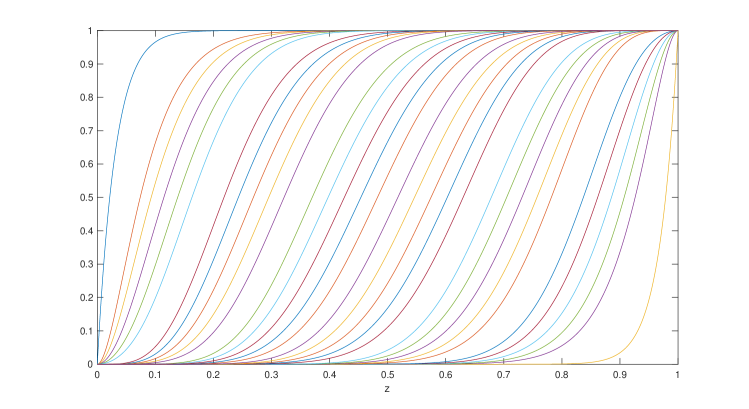
Figure 3: Polarization behavior of kernel $K_{32}$

4 Calculate the Polarization Behaviors

So far, we presented an algorithm to construct large binary kernels with intuitively good scaling exponents. In this section, we address the last challenge, which is to efficiently derive the polarization behavior of a given kernel. The NP hardness of this problem was previously established in [4]. In this section, we propose a few methods to reduce the computation complexity just enough so we can implement it. To this end, we present two trellis-based algorithms that can explicitly calculate the polarization behavior of $K_{32}$. Sadly, even these improved algorithms are beyond implementation for $K_{64}$. So, we present an alternative approach of “estimating” the polarization behavior of $K_{64}$ with high precision using a large but limited number of samples from the set of all erasure patterns. One can plug the estimated polarization behavior into the methods described in [5] and get $\mu(K_{64})\simeq 2.87$. We also provide a more careful analysis to show that $\mu(K_{64})\leqslant 2.9603$ rigorously.

4.1 Trellis Algorithms

A trellis is a graphical representation of a block code, in which every path represents a codeword. This representation allows us to do ML decoding with reduced complexity using the famous Viterbi algorithm. The Viterbi algorithm allows one to find the most likely path in a trellis. Besides decoding, it can also be generalized to find the weight distribution of the block code, given that the trellis is one-to-one. A trellis is called one-to-one if all of its paths are labeled distinctly. We refer the readers to [14] for the known facts about trellises we use in this section.

In this work, we develop new theory for trellis representation for the cover sets, which are both nonlinear and non-rectangular. We introduced two different algorithms that both can construct a one-to-one trellis for the cover set $\Delta(\mathcal{C}_{i-1}\backslash\mathcal{C}_{i})$. By efficiently representing the cover sets using trellises, we can use the Viterbi algorithm to calculate its weight distribution. A brief description of these algorithms together are given in the following. An example is also provided in Figure 5 for interested readers to track the steps in both algorithms.

1 for $i=0$ to $(\ell-1)$ do

2      for every vertex $v^{\ast}_{i}\in V^{\ast}_{i}$ do

3           for $a\in\{0,1\}$ do

4                calculate $s=$

5                $\{v_{i+1}\in V_{i+1}:\exists v_{i}\in L(v^{\ast}_{i}),(v_{i},v_{i+1},a)\in E\}$

6                if $\exists v^{\ast}_{i+1}\in V^{\ast}_{i+1}$ with $L(v^{\ast}_{i+1})=s$ then

7                     add an edge $(v^{\ast}_{i},v^{\ast}_{i+1},a)$ in $E^{\ast}$

8               else

9                     add a vertex $v^{\ast}_{i+1}\in V^{\ast}_{i+1}$ with $L(v^{\ast}_{i+1})=s$

10                     add an edge $(v^{\ast}_{i},v^{\ast}_{i+1},a)$ in $E^{\ast}$

11               

12          

13     

Algorithm 1 Construct a proper trellis $T^{\ast}$ from $T$

Proper Trellis Algorithm

A trellis is called proper if edges beginning at any given vertex are labeled distinctly. It is known that if a trellis is proper, then it is one-to-one. So, one way of constructing a one-to-one trellis for $\Delta(\mathcal{C}_{i-1}\backslash\mathcal{C}_{i})$ is to construct a proper trellis. The proper trellis algorithm has the following steps. Step 1: Construct a minimal trellis for the linear code $\mathcal{C}_{i}$. For every edges in $E_{i}$ where $i\in\mbox{supp}(g_{i})$, flip its label. We can then get a trellis for the coset $(\mathcal{C}_{i-1}\backslash\mathcal{C}_{i})$. Step 2. For every label-0 edges, add a parallel label-1 edge. Then we get a trellis representing the cover set $\Delta(\mathcal{C}_{i-1}\backslash\mathcal{C}_{i})$. But it is not a one-to-one trellis. Step 3. Let $T=(V,E,A)$ be the trellis we just constructed, use algorithm 1 to convert it into a proper trellis $T^{\ast}=(V^{\ast},E^{\ast},A)$, where for $i=0,1,2,\cdots,\ell$, vertices in $V^{\ast}_{i}$ are labeled uniquely by the subsets of $V_{i}$. $T^{\ast}$ will thus be a one-to-one trellis representing the same cover set $\Delta(\mathcal{C}_{i-1}\backslash\mathcal{C}_{i})$.

The proper trellis algorithm allows us to calculate the full polarization behavior of $K_{32}$, as shown in Figure 3. Unfortunately, the computational complexity is still too high for $K_{64}$, in which we were able to explicitly calculate the erasure probability polynomials associated with the last and first 15 rows in the kernel, as shown in Figure 4.

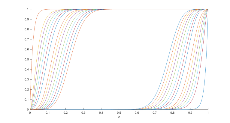
Figure 4: Polarization behavior of the first and the last 15 rows of kernel $K_{64}$

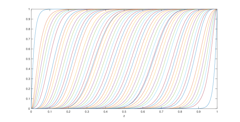
Figure 5: Polarization behavior of kernel $K_{64}$ by Monte Carlo interpolation method, where $1000$ values of $z$ are evaluated uniformly among $[0,1]$ with $N=10^{6}$.

Stitching Trellis Algorithm

The complexity of proper trellis algorithm depends on the number of vertices in the trellis. It’s difficult to predict the number of vertices for general kernels, which could be significantly large. Hence, we also propose an alternative approach which also constructs a one-to-one trellis for $\Delta(\mathcal{C}_{i-1}\backslash\mathcal{C}_{i})$, but has far less vertices. The stitching trellis algorithm differs from the proper trellis algorithm only by Step 3: Let $T=(V,E,A)$ be the trellis we just constructed, use algorithm 1 only for $i$ from 0 to $(\ell/2-1)$ to convert the first half of $T$ into a proper trellis $T_{1}$. Reverse algorithm 1 to convert the second half of $T$ into a co-proper trellis $T_{2}$. Let $V_{1},V_{2}$ be the vertex class of $T_{1},T_{2}$ at time $\ell/2$. Connect $T_{1}$ and $T_{2}$ by adding an edge $(v_{1},v_{2})$ with label 0 for every pair of vertices $v_{1}\in V_{1},v_{2}\in V_{2}$ where $L(v_{1})\cap L(v_{2})\neq 0$. Then the combined trellis, called stitching trellis, will be a one-to-one trellis representing the same cover set $\Delta(\mathcal{C}_{i-1}\backslash\mathcal{C}_{i})$.

The first and second half of the stitching trellis are proper and coproper respectively. Therefore, its number of vertices is bounded by $2^{\ell/2+1}$, which is far less than a proper trellis. Unfortunately, the naive way of stitching the middle segment requires a large amount of computation. We are still searching for a method to reduce its complexity and we believe this can be of independent interest to other researchers as well. Assuming such an efficient stitching is in place, the stitching trellis will be much more efficient than the proper trellis, which can also be used in other applications.

Figure 6: An example for the trellis algorithms. Top left: minimal trellis for $\mathcal{C}_{1}\backslash\mathcal{C}_{2}$ in $K_{4}=K_{2}^{\otimes 2}$; top right: step 2 of trellis algorithm; bottom left: step 3 of proper trellis algorithm; bottom right: step 3 of the stitching algorithm.

4.2 Monte Carlo Interpolation Method

As discussed earlier, the complexity of the trellis-based algorithms grow too high for the intermediate bit-channels of $K_{64}$. We present a Monte Carlo algorithm to estimate the values of polynomials $f_{i}(z)$ for any given $z\in(0,1)$. We recall again that $f_{i}(z)$ denotes the erasure probability of the $i$-th bit-channel $W_{i}$ given that the communication is taking place over a BEC$(z)$. A naive yet explicit approach to formulate $f_{i}(z)$ is to cross check all $2^{\ell}$ erasure patterns to discover the exact ratio of which become uncorrectable from $W_{i}$’s point of view. Instead, we propose to take $N$ samples of such erasure patterns and estimate the ratio accordingly. We recall that the computational complexity of determining “correctability” is no more than the complexity of a MAP decoder for the BEC, which is bounded by $O(\ell^{\omega})$, where $\omega$ is the exponent of matrix multiplication. Therefore, the overall complexity of the proposed approximation method can be bounded by $O(N\ell^{\omega})$. While this approach adds some uncertainty to our derivations, the numerical simulations suggest that $\hat{f}_{i}(z)$’s for $\forall i$ become visibly smooth and stable at $N=10^{6}$, as shown in Figure 5. The estimated value of $\mu(K_{64})\simeq 2.87$ is generated by invoking the recursive methods in [5] initialized with $\hat{f}_{i}(z)$’s for $\forall i$.

If the accurate values of $f_{i}(z)$ were known, one could use the bounding techniques in [5] to show that

$$\mu(K_{64})\leqslant-\bigg{(}{\log_{64}\bigg{(}\sup_{z\in(0,1)}\frac{\frac{1}{64}\sum_{i=1}^{64}g\big{(}f_{i}(z)\big{)}}{g(z)}\bigg{)}}\bigg{)}^{-1}$$ (6)

where $g(z)$ is a positive test function on $(0,1)$. However for kernel $K_{64}$, due to high computational complexity, 34 intermediate polarization bebavior polynomials are unknown. But we can still derive the strict upperbounds and lowerbounds for those unknown $f_{i}(z)$s’ to get the following theorem, with the proof in Appendix B.

Theorem 3.

$$\mu(K_{64})\leqslant 2.9603$$ (7)

Appendix A Kernels $K_{32}$ and $K_{64}$

$\left[\begin{array}[]{cccccccccccccccccccccccccccccccc}1&0&0&0&0&0&0&0&0&0&0&0&0&0&0&0&0&0&0&0&0&0&0&0&0&0&0&0&0&0&0&0\\ 1&0&0&0&0&0&0&0&0&0&0&0&0&0&0&0&0&0&0&0&0&0&0&0&0&0&0&0&0&0&1&0\\ 0&0&0&0&0&0&0&0&0&0&0&0&0&0&0&0&0&1&0&0&0&0&0&0&0&0&0&0&0&0&1&0\\ 0&0&0&0&0&0&0&0&0&0&0&0&0&0&0&0&0&0&0&0&0&0&0&0&1&0&0&0&0&0&1&0\\ 0&0&0&0&0&0&0&0&0&0&0&0&0&0&0&0&0&0&0&0&0&0&0&0&0&0&0&0&1&0&1&0\\ 1&0&0&1&0&0&0&0&0&0&0&0&0&0&0&0&0&0&0&0&0&0&0&0&0&0&0&0&1&0&1&0\\ 1&0&0&0&0&0&0&0&0&0&0&0&0&1&0&0&0&1&0&0&0&0&0&0&0&0&0&0&1&0&0&0\\ 1&0&0&0&0&0&1&0&0&0&0&0&0&0&0&0&0&0&0&0&0&0&0&0&1&0&0&0&0&0&1&0\\ 0&0&0&1&0&0&1&0&0&0&0&0&0&1&1&0&0&0&0&0&0&0&0&0&1&0&0&0&0&0&1&0\\ 1&0&0&1&0&0&1&0&0&0&0&0&0&1&0&0&0&1&0&0&0&0&0&0&0&0&0&1&1&0&1&0\\ 0&0&0&1&0&0&1&0&0&0&0&0&0&0&0&0&0&1&0&0&0&0&0&1&1&0&0&1&0&0&0&0\\ 1&0&0&1&0&0&1&0&0&0&0&0&0&0&1&0&0&0&0&0&0&1&0&0&0&0&0&0&0&0&1&0\\ 1&0&0&0&0&0&0&0&0&0&0&0&0&0&1&0&0&1&0&0&0&0&0&0&0&0&0&0&1&1&1&0\\ 1&0&0&1&0&0&0&0&0&0&0&0&0&0&0&0&0&0&0&0&0&0&0&0&1&0&1&0&1&1&0&0\\ 0&0&0&0&0&0&1&0&0&0&1&0&0&1&1&0&0&1&0&0&0&0&0&0&0&0&0&0&0&0&1&0\\ 1&0&0&0&0&0&1&0&0&0&0&0&0&1&1&0&0&0&0&0&1&1&0&0&0&0&0&1&1&1&1&0\\ 1&0&0&0&0&0&1&0&1&0&0&0&0&0&1&0&0&1&0&0&0&0&0&1&1&0&1&1&1&1&1&0\\ 1&0&0&1&0&0&0&0&0&0&0&0&0&1&1&0&1&1&0&0&0&1&0&1&1&0&1&0&1&1&0&0\\ 1&1&0&1&0&0&1&0&0&0&1&0&0&0&1&0&0&1&0&0&0&1&0&0&1&0&1&1&0&1&0&0\\ 1&0&1&1&0&0&1&0&0&0&1&0&0&1&0&0&0&1&0&0&1&1&0&1&0&0&1&0&0&1&0&0\\ 0&0&0&1&1&0&0&0&0&0&1&0&0&1&0&0&0&1&0&0&1&1&0&1&1&0&0&0&1&1&1&0\\ 1&1&1&1&0&0&0&0&0&1&1&0&0&1&1&0&0&0&0&0&0&0&0&0&1&0&0&1&0&1&1&0\\ 1&0&1&0&1&0&1&0&0&0&0&0&0&0&0&0&0&1&1&0&1&0&0&1&0&0&1&1&1&1&0&0\\ 0&1&1&0&1&1&0&0&1&0&1&0&0&0&0&0&0&0&0&0&0&1&0&1&0&0&1&1&0&1&1&0\\ 1&1&0&1&1&0&0&0&0&0&0&1&0&1&0&0&1&0&0&0&1&1&0&1&1&0&1&1&1&1&1&0\\ 0&0&0&1&0&0&1&0&1&0&0&0&0&1&0&0&0&1&0&0&0&1&1&1&0&0&1&0&1&1&1&0\\ 0&1&0&1&0&1&0&1&0&1&0&1&0&1&0&1&0&1&0&1&0&1&0&1&0&1&0&1&0&1&0&1\\ 0&0&1&1&0&0&1&1&0&0&1&1&0&0&1&1&0&0&1&1&0&0&1&1&0&0&1&1&0&0&1&1\\ 0&0&0&0&1&1&1&1&0&0&0&0&1&1&1&1&0&0&0&0&1&1&1&1&0&0&0&0&1&1&1&1\\ 0&0&0&0&0&0&0&0&1&1&1&1&1&1&1&1&0&0&0&0&0&0&0&0&1&1&1&1&1&1&1&1\\ 0&0&0&0&0&0&0&0&0&0&0&0&0&0&0&0&1&1&1&1&1&1&1&1&1&1&1&1&1&1&1&1\\ 1&1&1&1&1&1&1&1&1&1&1&1&1&1&1&1&1&1&1&1&1&1&1&1&1&1&1&1&1&1&1&1\\ \end{array}\right]$

Figure 7: Kernel $K_{32}$

$\left[\begin{array}[]{cccccccccccccccccccccccccccccccccccccccccccccccccccccccccccccccc}1&0&0&0&0&0&0&0&0&0&0&0&0&0&0&0&0&0&0&0&0&0&0&0&0&0&0&0&0&0&0&0&0&0&0&0&0&0&0&0&0&0&0&0&0&0&0&0&0&0&0&0&0&0&0&0&0&0&0&0&0&0&0&0\\ 1&0&0&0&0&0&0&0&0&0&0&0&0&0&0&0&0&0&0&0&0&0&0&0&0&0&0&0&0&0&0&0&1&0&0&0&0&0&0&0&0&0&0&0&0&0&0&0&0&0&0&0&0&0&0&0&0&0&0&0&0&0&0&0\\ 0&1&0&0&0&0&0&0&0&0&0&0&0&0&0&0&1&0&0&0&0&0&0&0&0&0&0&0&0&0&0&0&0&0&0&0&0&0&0&0&0&0&0&0&0&0&0&0&0&0&0&0&0&0&0&0&0&0&0&0&0&0&0&0\\ 0&0&1&0&0&0&0&0&1&0&0&0&0&0&0&0&0&0&0&0&0&0&0&0&0&0&0&0&0&0&0&0&0&0&0&0&0&0&0&0&0&0&0&0&0&0&0&0&0&0&0&0&0&0&0&0&0&0&0&0&0&0&0&0\\ 0&0&0&1&1&0&0&0&0&0&0&0&0&0&0&0&0&0&0&0&0&0&0&0&0&0&0&0&0&0&0&0&0&0&0&0&0&0&0&0&0&0&0&0&0&0&0&0&0&0&0&0&0&0&0&0&0&0&0&0&0&0&0&0\\ 0&0&0&0&1&0&1&0&0&0&0&0&0&0&0&0&0&0&0&0&0&0&0&0&0&0&0&0&0&0&0&0&0&0&0&0&0&0&0&0&0&0&0&0&0&0&0&0&0&0&0&0&0&0&0&0&0&0&0&0&0&0&0&0\\ 0&0&0&0&1&1&0&0&0&0&0&0&0&0&0&0&0&0&0&0&0&0&0&0&0&0&0&0&0&0&0&0&0&0&0&0&0&0&0&0&0&0&0&0&0&0&0&0&0&0&0&0&0&0&0&0&0&0&0&0&0&0&0&0\\ 0&1&0&1&1&0&1&0&0&0&0&0&0&0&0&0&0&0&0&0&0&0&0&0&0&0&0&0&0&0&0&0&0&0&0&0&0&0&0&0&0&0&0&0&0&0&0&0&0&0&0&0&0&0&0&0&0&0&0&0&0&0&0&0\\ 0&1&1&0&1&0&0&1&0&0&0&0&0&0&0&0&0&0&0&0&0&0&0&0&0&0&0&0&0&0&0&0&0&0&0&0&0&0&0&0&0&0&0&0&0&0&0&0&0&0&0&0&0&0&0&0&0&0&0&0&0&0&0&0\\ 0&1&0&1&1&1&0&0&1&0&0&1&0&0&0&0&0&0&0&0&0&0&0&0&0&0&0&0&0&0&0&0&0&0&0&0&0&0&0&0&0&0&0&0&0&0&0&0&0&0&0&0&0&0&0&0&0&0&0&0&0&0&0&0\\ 0&0&0&0&1&0&1&0&0&0&0&0&0&0&0&0&1&0&1&0&0&0&0&0&0&0&0&0&0&0&0&0&0&0&0&0&0&0&0&0&0&0&0&0&0&0&0&0&0&0&0&0&0&0&0&0&0&0&0&0&0&0&0&0\\ 0&1&0&1&0&0&0&0&1&0&1&0&0&0&0&0&0&0&0&0&0&0&0&0&0&0&0&0&0&0&0&0&0&0&0&0&0&0&0&0&0&0&0&0&0&0&0&0&0&0&0&0&0&0&0&0&0&0&0&0&0&0&0&0\\ 0&0&0&1&1&1&1&0&1&0&0&0&1&0&0&0&0&0&0&0&0&0&0&0&0&0&0&0&0&0&0&0&0&0&0&0&0&0&0&0&0&0&0&0&0&0&0&0&0&0&0&0&0&0&0&0&0&0&0&0&0&0&0&0\\ 0&1&0&0&0&1&0&0&0&1&0&0&1&0&0&0&1&1&0&0&0&0&0&0&0&0&0&0&0&0&0&0&0&0&0&0&0&0&0&0&0&0&0&0&0&0&0&0&0&0&0&0&0&0&0&0&0&0&0&0&0&0&0&0\\ 0&0&1&1&1&0&1&0&0&0&0&0&0&1&1&0&0&0&0&0&0&0&0&0&0&0&0&0&0&0&0&0&0&0&0&0&0&0&0&0&0&0&0&0&0&0&0&0&0&0&0&0&0&0&0&0&0&0&0&0&0&0&0&0\\ 0&0&0&1&1&1&0&0&0&0&1&0&0&0&0&0&1&0&0&0&0&0&0&0&1&0&0&0&0&0&0&0&0&0&0&0&0&0&0&0&0&0&0&0&0&0&0&0&0&0&0&0&0&0&0&0&0&0&0&0&0&0&0&0\\ 0&0&0&0&0&0&1&0&0&1&1&0&0&0&0&1&1&1&1&0&0&0&0&0&1&0&0&0&0&0&0&0&1&1&0&0&0&0&0&0&0&0&0&0&0&0&0&0&0&0&0&0&0&0&0&0&0&0&0&0&0&0&0&0\\ 0&0&1&0&1&1&1&0&0&0&1&0&1&0&0&0&1&1&0&0&0&0&0&0&0&0&0&0&0&0&0&0&1&0&1&0&0&0&0&0&0&0&0&0&0&0&0&0&0&0&0&0&0&0&0&0&0&0&0&0&0&0&0&0\\ 0&0&1&1&0&0&1&0&1&0&0&0&0&0&0&0&0&1&0&0&0&0&0&0&1&0&0&0&0&0&0&0&0&0&1&0&1&0&0&0&0&0&0&0&0&0&0&0&0&0&0&0&0&0&0&0&0&0&0&0&0&0&0&0\\ 0&0&0&1&1&1&1&0&1&1&1&0&0&0&0&0&0&0&0&0&0&0&0&0&1&0&0&0&0&0&0&0&0&1&1&0&1&0&0&0&0&0&0&0&0&0&0&0&1&0&0&0&0&0&0&0&0&0&0&0&0&0&0&0\\ 0&1&1&0&1&0&0&1&1&1&1&0&1&0&0&0&0&0&0&1&0&0&0&0&1&0&0&0&0&0&0&0&0&0&0&0&1&0&0&0&1&0&0&0&0&0&0&0&0&0&0&0&0&0&0&0&0&0&0&0&0&0&0&0\\ 0&0&1&1&1&0&1&0&0&1&0&0&1&0&0&0&1&1&1&0&0&1&0&0&0&0&0&0&0&0&0&0&0&0&0&0&0&0&0&0&0&0&0&0&0&0&0&0&0&0&0&0&0&0&0&0&0&0&0&0&0&0&0&0\\ 0&1&0&1&1&0&1&0&0&0&1&1&1&1&0&0&0&1&1&0&0&1&1&0&0&0&0&0&0&0&0&0&0&0&0&0&0&0&0&0&0&0&0&0&0&0&0&0&0&0&0&0&0&0&0&0&0&0&0&0&0&0&0&0\\ 0&1&0&1&1&0&1&0&1&1&0&0&1&1&0&0&0&1&1&0&1&0&0&1&0&0&0&0&0&0&0&0&0&0&0&0&0&0&0&0&0&0&0&0&0&0&0&0&0&0&0&0&0&0&0&0&0&0&0&0&0&0&0&0\\ 0&0&0&0&0&0&0&0&1&0&0&1&0&1&1&0&0&1&1&0&1&0&0&1&0&0&0&0&0&0&0&0&0&0&0&0&0&0&0&0&0&0&0&0&0&0&0&0&0&0&0&0&0&0&0&0&0&0&0&0&0&0&0&0\\ 1&1&0&0&0&0&0&0&1&1&0&0&0&0&0&0&1&1&0&0&0&0&0&0&1&1&0&0&0&0&0&0&0&0&0&0&0&0&0&0&0&0&0&0&0&0&0&0&0&0&0&0&0&0&0&0&0&0&0&0&0&0&0&0\\ 0&1&0&0&0&1&1&1&0&1&0&0&0&1&1&1&1&0&0&0&0&1&0&0&1&0&0&0&0&1&0&0&0&0&0&0&0&0&0&0&0&0&0&0&0&0&0&0&0&0&0&0&0&0&0&0&0&0&0&0&0&0&0&0\\ 0&0&1&0&1&1&1&0&0&1&0&0&1&0&0&0&1&1&1&0&0&0&1&0&1&0&0&0&0&1&0&0&0&0&0&0&0&0&0&0&0&0&0&0&0&0&0&0&0&0&0&0&0&0&0&0&0&0&0&0&0&0&0&0\\ 0&0&0&0&0&1&1&0&0&1&0&1&1&1&0&0&1&1&0&0&1&0&1&0&1&0&0&1&0&0&0&0&0&0&0&0&0&0&0&0&0&0&0&0&0&0&0&0&0&0&0&0&0&0&0&0&0&0&0&0&0&0&0&0\\ 0&1&1&0&0&1&1&0&1&0&0&1&0&1&1&0&0&0&1&1&1&1&0&0&1&1&0&0&1&1&0&0&0&0&0&0&0&0&0&0&0&0&0&0&0&0&0&0&0&0&0&0&0&0&0&0&0&0&0&0&0&0&0&0\\ 0&0&1&1&0&1&1&0&1&1&0&0&1&0&0&1&1&1&0&0&0&1&1&0&1&1&0&0&0&1&1&0&0&0&0&0&0&0&0&0&0&0&0&0&0&0&0&0&0&0&0&0&0&0&0&0&0&0&0&0&0&0&0&0\\ 0&1&0&1&1&1&0&0&1&0&0&1&0&0&0&0&0&1&0&1&1&1&0&0&0&1&1&0&0&0&0&0&1&1&1&1&0&0&0&0&0&0&0&0&0&0&0&0&0&0&0&0&0&0&0&0&0&0&0&0&0&0&0&0\\ 0&0&0&0&0&0&0&1&1&0&0&1&0&0&1&0&0&1&0&0&0&1&1&0&1&0&0&0&0&0&0&0&0&0&0&1&0&1&1&0&0&0&1&0&0&0&0&0&0&1&1&0&0&0&1&0&0&0&0&0&0&0&0&1\\ 0&1&1&0&1&1&0&0&0&0&1&1&0&0&0&0&0&0&1&1&0&0&0&0&0&1&0&1&0&0&0&0&0&0&1&1&1&1&0&0&0&1&1&0&0&0&0&0&0&1&1&0&0&0&0&0&0&0&0&0&0&0&0&0\\ 0&0&0&0&1&0&0&1&0&0&0&0&1&0&1&0&0&0&0&0&0&1&1&0&0&1&0&1&0&0&0&0&0&0&0&1&1&1&1&0&0&1&0&0&1&0&0&0&0&0&1&0&0&0&1&0&0&0&1&0&0&0&0&1\\ 0&0&1&0&0&1&0&0&1&0&0&1&0&0&0&0&0&0&1&1&1&1&0&0&0&1&0&0&0&1&0&0&0&0&0&1&0&1&0&0&0&1&1&0&1&1&0&0&0&1&1&0&1&0&1&0&0&0&1&0&0&0&0&1\\ 0&1&0&0&0&0&0&1&1&1&0&0&1&0&1&0&0&1&0&0&1&0&0&0&0&0&0&0&0&0&0&0&0&0&0&0&0&1&1&0&1&1&1&0&0&1&0&0&0&0&0&0&0&0&0&0&0&0&1&0&0&0&0&1\\ 0&0&1&0&0&0&0&0&0&0&0&1&1&0&1&0&1&1&1&1&1&0&0&0&0&1&0&1&0&1&0&0&0&0&1&0&0&0&0&0&0&1&0&0&0&0&0&0&0&0&0&0&1&0&0&0&0&0&0&0&0&0&0&1\\ 0&0&0&0&1&1&0&0&0&0&0&0&0&0&0&0&0&0&0&1&0&0&1&0&0&1&0&0&0&1&0&0&0&1&1&0&0&1&1&0&1&1&0&0&0&0&0&0&0&0&1&0&0&0&1&0&0&0&1&0&0&0&0&1\\ 0&0&0&1&1&0&0&0&0&1&1&1&1&0&0&0&1&0&0&1&0&0&0&0&0&0&0&0&0&0&0&0&0&0&0&0&1&0&1&0&0&0&0&0&1&1&0&0&0&0&1&0&1&0&0&0&0&0&1&0&0&0&0&1\\ 0&0&0&0&0&0&1&0&1&1&0&0&1&0&0&0&0&0&1&0&0&1&1&0&1&1&0&1&0&0&0&0&0&1&0&0&1&0&1&0&1&0&0&0&0&0&0&0&0&0&0&0&1&0&0&0&0&0&0&0&0&0&0&1\\ 0&0&0&1&0&0&0&0&1&0&0&0&1&1&0&0&1&1&1&0&0&0&0&0&0&1&0&0&0&0&0&0&0&0&0&0&0&1&0&0&1&0&1&0&0&1&0&0&0&1&1&0&0&0&1&0&0&0&0&0&0&0&0&1\\ 0&1&0&0&0&1&1&1&0&0&1&0&1&1&1&0&1&1&1&0&0&0&1&0&0&1&1&1&0&1&0&0&0&0&0&1&0&0&1&0&1&0&0&0&0&1&0&0&0&1&0&0&1&0&0&0&0&0&1&0&0&0&0&1\\ 0&0&1&0&0&0&0&1&0&0&1&0&1&1&1&0&1&0&0&0&0&1&0&0&0&1&1&1&0&1&0&0&0&1&1&1&0&1&0&0&1&0&0&0&0&1&0&0&0&0&1&0&1&1&1&0&0&0&1&0&0&0&0&1\\ 0&0&0&1&1&1&0&1&0&0&0&1&0&0&1&0&1&0&0&0&0&1&0&0&0&1&1&1&0&1&0&0&0&1&0&0&1&0&0&0&1&0&1&1&1&0&0&0&0&0&1&0&1&1&1&0&0&0&1&0&0&0&0&1\\ 0&0&0&1&0&0&1&0&1&1&1&0&0&0&1&0&1&0&0&0&1&0&1&1&1&0&0&0&0&1&0&0&0&1&0&0&1&0&0&0&1&0&1&1&1&0&0&0&0&0&1&0&1&1&1&0&0&0&1&0&0&0&0&1\\ 0&0&0&1&0&0&1&0&1&0&0&0&0&1&0&0&1&1&1&0&1&1&0&1&1&0&0&0&0&1&0&0&0&1&0&0&1&0&0&0&1&1&0&1&1&1&1&0&0&1&0&0&1&0&0&0&0&0&1&0&0&0&0&1\\ 0&0&0&1&0&0&1&0&1&0&0&0&0&1&0&0&1&1&0&1&0&0&0&1&1&0&1&1&1&0&0&0&0&1&1&1&0&1&0&0&1&1&1&0&0&0&1&0&0&1&0&0&1&0&0&0&0&0&1&0&0&0&0&1\\ 0&1&1&1&0&0&1&0&1&0&0&0&0&0&1&0&1&1&0&1&0&1&1&1&1&1&0&1&1&0&0&0&0&0&0&1&0&1&0&0&1&1&1&0&0&1&0&0&0&1&0&0&1&1&1&0&0&1&0&0&0&0&0&1\\ 0&0&1&0&0&1&1&1&0&0&0&1&0&1&0&0&1&1&0&1&1&0&0&0&0&0&0&1&0&1&0&0&0&1&1&1&0&0&1&0&1&0&1&1&1&1&1&0&0&1&1&1&0&0&1&0&0&1&0&0&0&0&0&1\\ 0&0&0&1&1&1&0&1&0&0&1&0&1&1&1&0&1&0&0&0&1&0&1&1&1&0&1&1&1&0&0&0&0&1&1&1&1&0&1&1&0&1&0&0&1&0&0&0&0&0&0&1&0&0&1&0&0&0&1&0&0&0&0&1\\ 0&0&0&1&1&0&1&1&1&1&1&0&1&0&1&1&0&0&0&1&0&1&0&0&1&1&1&0&0&1&0&0&0&1&0&0&0&0&0&1&0&1&0&0&1&1&1&0&0&1&0&0&1&1&1&0&0&1&0&0&0&0&0&1\\ 0&0&0&1&0&0&1&0&0&1&0&0&0&1&1&1&0&1&1&1&0&1&0&0&1&1&0&1&1&1&1&0&0&0&0&1&0&0&1&0&1&0&1&1&1&0&0&0&0&1&1&1&0&1&0&0&0&0&1&0&0&0&0&1\\ 0&0&0&0&0&0&1&1&0&0&0&0&1&1&0&0&1&0&1&0&1&0&0&1&1&0&1&0&0&1&1&0&0&0&1&1&1&1&1&1&0&0&1&1&0&0&0&0&0&1&1&0&1&0&1&0&0&1&1&0&0&1&0&1\\ 0&1&0&0&0&0&1&0&0&0&1&0&1&0&1&1&0&0&1&0&0&1&0&0&1&0&1&1&0&0&1&0&0&1&1&1&1&1&1&0&1&1&1&0&1&0&0&0&0&0&0&1&1&0&0&0&0&1&1&1&0&0&0&1\\ 0&0&1&1&1&0&0&1&1&0&0&1&1&1&0&0&1&0&0&1&1&1&0&0&1&1&0&0&0&1&1&0&0&0&0&0&0&1&0&1&1&0&1&0&0&0&0&0&0&1&0&1&1&1&1&1&0&0&0&0&0&1&0&1\\ 0&0&0&0&0&1&1&0&0&1&0&1&0&0&1&1&1&1&0&0&1&0&1&0&0&1&1&0&0&0&0&0&0&1&0&1&0&0&1&1&1&1&1&1&1&0&0&1&0&1&1&0&0&0&0&0&0&0&1&1&0&1&0&1\\ 0&1&0&1&0&1&0&1&0&1&0&1&0&1&0&1&0&1&0&1&0&1&0&1&0&1&0&1&0&1&0&1&0&1&0&1&0&1&0&1&0&1&0&1&0&1&0&1&0&1&0&1&0&1&0&1&0&1&0&1&0&1&0&1\\ 0&0&1&1&0&0&1&1&0&0&1&1&0&0&1&1&0&0&1&1&0&0&1&1&0&0&1&1&0&0&1&1&0&0&1&1&0&0&1&1&0&0&1&1&0&0&1&1&0&0&1&1&0&0&1&1&0&0&1&1&0&0&1&1\\ 0&0&0&0&1&1&1&1&0&0&0&0&1&1&1&1&0&0&0&0&1&1&1&1&0&0&0&0&1&1&1&1&0&0&0&0&1&1&1&1&0&0&0&0&1&1&1&1&0&0&0&0&1&1&1&1&0&0&0&0&1&1&1&1\\ 0&0&0&0&0&0&0&0&1&1&1&1&1&1&1&1&0&0&0&0&0&0&0&0&1&1&1&1&1&1&1&1&0&0&0&0&0&0&0&0&1&1&1&1&1&1&1&1&0&0&0&0&0&0&0&0&1&1&1&1&1&1&1&1\\ 0&0&0&0&0&0&0&0&0&0&0&0&0&0&0&0&1&1&1&1&1&1&1&1&1&1&1&1&1&1&1&1&0&0&0&0&0&0&0&0&0&0&0&0&0&0&0&0&1&1&1&1&1&1&1&1&1&1&1&1&1&1&1&1\\ 0&0&0&0&0&0&0&0&0&0&0&0&0&0&0&0&0&0&0&0&0&0&0&0&0&0&0&0&0&0&0&0&1&1&1&1&1&1&1&1&1&1&1&1&1&1&1&1&1&1&1&1&1&1&1&1&1&1&1&1&1&1&1&1\\ 1&1&1&1&1&1&1&1&1&1&1&1&1&1&1&1&1&1&1&1&1&1&1&1&1&1&1&1&1&1&1&1&1&1&1&1&1&1&1&1&1&1&1&1&1&1&1&1&1&1&1&1&1&1&1&1&1&1&1&1&1&1&1&1\end{array}\right]$

Figure 8: Kernel $K_{64}$

Appendix B Proof for Theorem 3

Given an $\ell\times\ell$ kernel with polarization behavior $\{f_{1},\cdots,f_{\ell}\}$, for a fixed $z\in[0,1]$, we can define the process

$$Z_{0}=z,\qquad Z_{n+1}=\begin{cases}f_{1}(Z_{n})&\text{w.p. }1/\ell\\ f_{2}(Z_{n})&\text{w.p. }1/\ell\\ \vdots&\vdots\\ f_{1}(Z_{n})&\text{w.p. }1/\ell\\ \end{cases}$$ (8)

First lets recall the scaling assumption

Assumption 1.

There exists $\mu\in(0,\infty)$ such that, for any $z,a,b\in(0,1)$ such that $a<b$, The limit $\lim_{n\rightarrow\infty}\ell^{\frac{n}{\mu}}\text{Pr}(Z_{n}\in[a,b])$ exists in $(0,\infty)$.

For a generic test function $g:[0,1]\rightarrow[0,1]$, define the sequence of functions $\{g_{n}\}_{n\in\mathbb{N}}$ as $g_{n}:[0,1]\rightarrow[0,1]$ that

$$g_{n}(z)=\mathbb{E}[g(Z_{n})\mid Z_{0}=z]$$ (9)

Then this sequence of functions satisfies the recursive relation

$$g_{0}(z)=g(z),\qquad g_{n+1}(z)=\frac{1}{\ell}\sum_{i=1}^{\ell}g_{n}(f_{i}(z))$$ (10)

Our approach of bounding $\mu(K_{64})$ has the following steps: (1) Find a suitable test function $g(z)$; (2) provide an upperbound on the polarizing speed of the sequence $\{g_{n}(z)\}_{n\in\mathbb{N}}$ and (3) turn this upperbound into bound for $\mu(K_{64})$. We here define the sequence $\{b_{n}\}_{n\in\mathbb{N}}$ to measure the polarizing speed of $\{g_{n}(z)\}_{n\in\mathbb{N}}$.

Definition 4.

$$b_{n}(z)=\frac{g_{n+1}(z)}{g_{n}(z)},\qquad b_{n}=\sup_{z\in(0,1)}b_{n}(z)$$

We can prove that $\{b_{n}\}_{n\in\mathbb{N}}$ is a decreasing sequence.

Lemma 2.

$\{b_{n}\}_{n\in\mathbb{N}}$ is a decreasing sequence.

Proof.

Since for any fixed $z$

$$g_{n+1}(z) =\frac{1}{\ell}\sum_{i=1}^{\ell}g_{n}(f_{i}(z))$$

$$\leqslant b_{n-1}\left(\frac{1}{\ell}\sum_{i=1}^{\ell}g_{n-1}(f_{i}(z))\right)$$

$$=b_{n-1}\cdot g_{n}(z)$$

We have $b_{n}(z)=\frac{g_{n+1}(z)}{g_{n}(z)}\leqslant b_{n-1}$ for any $z$. Therefore $b_{n}\leqslant b_{n-1}$ and $\{b_{n}\}_{n\in\mathbb{N}}$ is a decreasing sequence. ∎

From the above lemma we have:

$$g_{n}(z) \leqslant b_{n-1}g_{n-1}(z)$$

$$\leqslant b_{0}g_{n-1}(z)$$

$$\leqslant\cdots$$

$$\leqslant b^{n}_{0}g(z)$$

Next we use $b_{0}$ to give an upperbound for the scaling exponent of the kernel.

Lemma 3.

For $a,b\in(0,1)$ and $n\in\mathbb{N}$ we have:

$$\frac{1}{n}\log_{\ell}\text{Pr}(Z_{n}\in[a,b])\leqslant\log_{\ell}b_{0}+O\left(\frac{1}{n}\right)$$

Proof.

By Markov inequality

$$\text{Pr}(Z_{n}\in[a,b]) \leqslant\text{Pr}(g(Z_{n})\geqslant\min_{z\in[a,b]}g(z))$$

$$\leqslant\frac{\mathbb{E}[g(Z_{n})]}{\min_{z\in[a,b]}g(z)}$$

So

$$\frac{1}{n}\log_{\ell}\text{Pr}(Z_{n}\in[a,b]) \leqslant\frac{1}{n}\log_{\ell}\frac{(b_{0})^{n}g(z)}{\min_{z\in[a,b]}g(z)}$$

$$\leqslant\log_{\ell}b_{0}+\frac{1}{n}\left(\log_{\ell}\frac{g(z)}{\min_{z\in[a,b]}g(z)}\right)$$

∎

Since by scaling assumption

$$-\frac{1}{\mu}=\lim_{n\rightarrow\infty}\frac{1}{n}\log_{\ell}(\text{Pr}(Z_{n}\in[a,b]))$$

We have $\mu\leqslant-\frac{1}{\log_{\ell}b_{0}}$. We next pick the appropriate test function $g$ and use $b_{0}$ to obtain a valid upperbound for $\mu(K_{64})$. First we explain in detail how we construct this test function $g(z)$.

By the trellis algorithm, we get the explicit polynomials $f_{50},\cdots,f_{64}$. By the duality theorem, we also get to know the explicit formulas for $f_{1},\cdots,f_{15}$. And there are 34 polarization behavior polynomials left unknown. But for those unknown coefficients, we can calculate their upperbound as follows:

Lemma 4.

Let $A_{0},A_{1},\cdots,A_{\ell}$ be the weight enumerators for the coset $(C_{i-1}\backslash C_{i})$, then

$$E_{i,w}\leqslant\min\left(\sum_{j=1}^{i}\binom{\ell-i}{j-i}A_{i},\binom{\ell}{i}\right)$$

Proof.

By theorem 1 any erasure pattern is uncorrectable iff it covers a codeword in $(C_{i-1}\backslash C_{i})$. For each codeword in $(C_{i-1}\backslash C_{i})$ of weight $j$, there are $\binom{n-j}{w-j}$ erasure patterns with weight $w$ that covers it. So $E_{i,w}\leqslant\sum_{j=1}^{i}\binom{\ell-i}{j-i}A_{i}$. On the other hand, $E_{i,w}$ is at most $\binom{\ell}{i}$. ∎

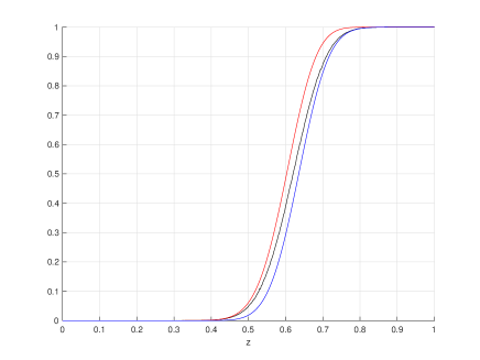
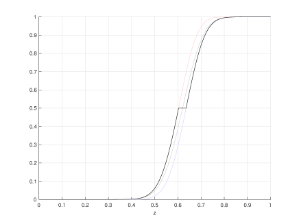
Figure 9: For kernel $K_{64}$, on the left, from left to right we have $\overline{f}_{40}(z)$, $f_{40}(z)$ simulated by Monte Carlo interpolation method and $\underline{f}_{40}(z)$. On the right we have, $\tilde{f}_{40}(z)$.

For $i=16,17,\cdots,49$ of $K_{64}$. Define

$$\overline{E}_{i,w}=\min\left(\sum_{j=1}^{i}\binom{\ell-i}{j-i}A_{i},\binom{\ell}{i}\right),\quad\underline{E}_{i,w}=\binom{\ell}{i}-\overline{E}_{\ell+1-i,\ell-w}$$

And define

$$\overline{f}_{i}(z)=\sum_{i=0}^{\ell}\overline{E}_{i,w}z^{i}(1-z)^{\ell-i},\qquad\underline{f}_{i}(z)=\sum_{i=0}^{\ell}\underline{E}_{i,w}z^{i}(1-z)^{\ell-i}$$

Then for $i=16,17,\cdots,49$ and any fixed $z$, $f_{i}(z)\in[\overline{f}_{i}(z),\underline{f}_{i}(z)]$. An example for $\overline{f}_{i}(z)$ and $\underline{f}_{i}(z)$ are shown in Fig 9.

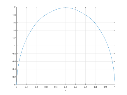
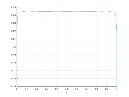
Figure 10: Left: test function $g(z)$. Right: upperbound $\overline{b}_{0}(z)$.

We define our test function $g$ as follows

$$g(z)=\frac{1}{64}\left(\sum_{i=1}^{15}g^{\ast}(f_{i}(z))+\sum_{i=50}^{64}g^{\ast}(f_{i}(z))+\sum_{i=16}^{49}g^{\ast}(\tilde{f}_{i}(z))\right),\qquad g^{\ast}(z)=z^{1/2}(1-z)^{1/2}$$

where

$$\tilde{f}_{i}(z)=\begin{cases}\overline{f}_{i}(z)&\overline{f}_{i}(z)\leqslant 0.5\\ 0.5&0.5\in(\overline{f}_{i}(z),\underline{f}_{i}(z))\\ \underline{f}_{i}(z)&\underline{f}_{i}(z)\geqslant 0.5\\ \end{cases}$$

An example of $\tilde{f}_{i}(z)$ is shown in Fig 9. And a plot of the test function is shown in Fig 10. Since $K_{64}$ is self-dual, by duality theorem we can shown that $g(z)$ increases on $[0,0.5]$, decreases on $[0.5,1]$, and reach its maximum when $z=0.5$. Therefore for $i=16,17,\cdots,49$:

$$g(f_{i}(z))\leqslant\begin{cases}g(\overline{f}_{i}(z))&\overline{f}_{i}(z)\leqslant 0.5\\ g(0.5)&0.5\in(\overline{f}_{i}(z),\underline{f}_{i}(z))\\ g(\underline{f}_{i}(z))&\underline{f}_{i}(z)\geqslant 0.5\\ \end{cases}$$

And this gives us a strict upper bound $\overline{g}_{1}(z)$ for $g_{1}(z)$:

$$g_{1}(z) =\frac{1}{64}\left(\sum_{i=1}^{64}g(f_{i}(z))\right)\quad\leqslant\quad\overline{g}_{1}(z)=\frac{1}{64}\left(\sum_{i=1}^{15}g(f_{i}(z))+\sum_{i=50}^{64}g(f_{i}(z))+\sum_{i=16}^{49}g(\tilde{f}_{i}(z))\right)$$

which provide a strict upper bound $\overline{b}_{0}(z)$ for $b_{0}(z)$, as shown in Fig 10

$$b_{0}(z)=\frac{g_{1}(z)}{g(z)}\quad\leqslant\quad\overline{b}_{0}(z)=\frac{\overline{g}_{1}(z)}{g(z)}$$

And the maximum value of $\overline{b}_{0}(z)$ can be calculated analytically up to any desired precision. Our calculation shows that:

$$b_{0}=\sup_{z\in(0,1)}b_{0}(z)\leqslant\max_{z\in(0,1)}\overline{b}_{0}(z)=0.2454$$

which provides an upperbound $\mu(K_{64})\leqslant-\frac{1}{\log_{64}0.2454}=2.9603$.

References

- [1] E. Arıkan, “Channel polarization: A method for constructing capacity achieving codes for symmetric binary-input memoryless channels,” IEEE Transactions on Information Theory, vol. 55, no. 7, pp. 3051–73, 2009.
- [2] S. Buzaglo, A. Fazeli, P. H. Siegel, V. Taranalli, and A. Vardy, “Permuted successive cancellation decoding for polar codes,” In Proc. of IEEE International Symposium on Information Theory, pp. 2618–22, 2017.
- [3] A. Fazeli, S. H. Hassani, M. Mondelli, and A. Vardy, “Binary linear codes with optimal scaling and quasi-linear complexity,” [Online] arXiv preprint arXiv:1711.01339. 2017.
- [4] A. Fazeli and A. Vardy. “On the scaling exponent of binary polarization kernels”, In Proceedings of Allerton Conference on Communication, Control, and Computing, pp. 797–804, 2014.
- [5] H. S. Hassani, K. Alishahi, and R. L. Urbanke, “Finite-length scaling of polar codes,” IEEE Transactions on Information Theory, vol. 60, no. 10, pp. 5875–98, 2014.
- [6] S. B. Korada, E. Şaşoğlu, and R. Urbanke, “Polar codes: Characterization of exponent, bounds, and constructions,” IEEE Transactions on Information Theory, vol. 56, no. 12, pp. 6253–64, 2010.
- [7] H. Mahdavifar, “Fast polarization and finite-length scaling for non-stationary channels,” [Online] arXiv preprint arXiv:1611.04203. 2016.
- [8] M. Mondelli, S. H. Hassani, and R. L. Urbanke, “Unified scaling of polar codes: Error exponent, scaling exponent, moderate deviations, and error floors,” IEEE Transactions on Information Theory, vol. 62, no. 12, pp. 6698-712, 2016.
- [9] V. Miloslavskaya and P. Trifonov, “Design of binary polar codes with arbitrary kernel,” In Proceedings of IEEE Information Theory Workshop, pp. 119–123, 2012.
- [10] H. D. Pfister and R. Urbanke, “Near-optimal finite-length scaling for polar codes over large alphabets,” In Proceedings of IEEE International Symposium on Information Theory (ISIT), pp. 215–219, 2016.
- [11] Y. Polyanskiy, H. V. Poor, and S. Verdu, “Channel coding rate in the finite blocklength regime,” IEEE Transactions on Information Theory, vol. 56, no. 5, pp. 2307–59, 2010.
- [12] V. Strassen, “Asymptotische Abschatzungen in Shannon’s Informationstheorie,” Prague Conference on Information Theory, Statistical Decision Functions, and Random Processes, pp. 689–723, 1962.
- [13] G. Trofimiuk, P. Trifonov, “Efficient decoding of polar codes with some kernels,” 2018 IEEE Information Theory Workshop (ITW). IEEE, 2018.
- [14] A. Vardy, “Trellis structure of codes,” in Handbook of Coding Theory, Elsevier, 1998.