Sitatapatra: Blocking the Transfer of Adversarial Samples

Abstract

Convolutional Neural Networks (CNNs) are widely used to solve classification tasks in computer vision. However, they can be tricked into misclassifying specially crafted “adversarial” samples – and samples built to trick one model often work alarmingly well against other models trained on the same task. In this paper we introduce Sitatapatra, a system designed to block the transfer of adversarial samples. We show how Sitatapatra has the potential to serve as a key and diversifies neural networks, as in cryptography, and provides a mechanism for detecting attacks. What’s more, when adversarial samples are detected they can typically be traced back to the individual device that was used to develop them. The run-time overheads are minimal permitting the use of Sitatapatra on constrained systems.

1 Introduction

Convolutional Neural Networks (CNNs) have achieved revolutionary performance in vision-related tasks such as segmentation [3], image classification [17], object detection [30] and visual question answering [2]. It is now inevitable that CNNs will be deployed widely for a broad range of applications including both safety-critical and security-critical tasks such as autonomous vehicles [7], face recognition [31] and action recognition [13].

However, researchers have discovered that small perturbations to input images can trick CNNs — with classifiers producing results surprisingly far from the correct answer in response to small perturbations that are not perceptible by humans. An attacker can thus create adversarial image inputs that cause a CNN to misbehave. The resulting attack scenarios are broad, ranging from breaking into smartphones through face-recognition systems [4] to misdirecting autonomous vehicles through perturbed road signs [6].

The attacks are also practical, because they are surprisingly portable. If devices are shipped with the same CNN classifier, the attacker only needs to analyze a single one of them to perform effective attacks on the others. Imagine a firm that deploys the same CNN on devices in very different environments. An attacker might not be able to experiment with a security camera in a bank vault, but if a cheaper range of security cameras are sold for home use and use the same CNN, he may buy one and generate transferable adversarial samples using it. What is more, making CNNs sufficiently different is not straightforward. Recent research teaches that different CNNs trained to solve similar problems are often vulnerable to the same adversarial samples [27, 37]. It is clear that we need an efficient way of limiting the transferability of adversarial samples. And given the complexity of the scenarios in which sensors operate, the protection mechanism should: a) work in computationally constrained environments; b) require minimal changes to the model architecture, and; c) offer a way of building complex security policies.

In this paper we propose Sitatapatra, a system designed and built to constrain the transferability of adversarial examples. Inspired by cryptography, we introduce a notion of key into CNNs that causes each network of the same architecture to be internally different enough to stop the transferability of adversarial attacks. We describe multiple ways of embedding the keys and evaluate them extensively on a range of computer vision benchmarks. Based on these data, we propose a scheme to pick keys. Finally, we discuss the scalability of the Sitatapatra defence and describe the trade-offs inherent in its design.

The contributions of this paper are:

• We introduce Sitatapatra, the first system designed to stop adversarial samples being transferable.

• We describe how to embed a secret key into CNNs.

• We show that Sitatapatra not only blocks sample transfer, but also allows detection and attack attribution.

• We measure performance and show that the run-time computational overhead is low enough (0.6–7%) for Sitatapatra to work on constrained devices.

The paper is structured as follows. Section 2 describes the related work. Section 3 introduces the methodology of Sitatapatra and presents the design choices. Section 4 evaluates the system against state-of-the-art attacks on three popular image classification benchmarks. Section 5 discusses the trade-offs in Sitatapatra, analyses key diversity and the costs of key change, and discusses how to deploy Sitatapatra effectively at scale.

2 Related Work

Since the invention of adversarial attacks against CNNs [33], there has been rapid co-evolution of attack and defense techniques in the deep learning community.

An adversarial sample is defined as a slightly perturbed image $\hat{\mathbf{x}}$ of the original $\mathbf{x}$, while $\hat{\mathbf{x}}$ and $\mathbf{x}$ are assigned different classes by a CNN classifier $F$. The $l^{p}$-norm of the perturbation is often constrained by a small constant $\epsilon$ such that ${\|\hat{\mathbf{x}}-\mathbf{x}\|}_{p}\leq\epsilon$ and $0\leq\hat{\mathbf{x}}\leq 1$, where $p$ can be 1, 2, or $\infty$.

The fast gradient sign method (FGSM) [9] is a simple and effective $L^{\infty}$ attack for finding such samples. FGSM generates $\hat{\mathbf{x}}$ by computing the gradient of the target class $y$ with respect to $\mathbf{x}$, and applies a distortion $\epsilon$ for all pixels against the sign of the gradient direction:

$$\hat{\mathbf{x}}=\mathrm{clip}\left(\mathbf{x}+\epsilon\cdot\mathrm{sign}\left(\nabla_{\mathbf{x}}\ell_{y}\left(F\left(x\right)\right)\right)\right),$$ (1)

where $\ell_{y}(F(\mathbf{x}))$ denotes the loss of the network output $F(\mathbf{x})$ for the target class $y$, $\nabla_{\mathbf{x}}(\mathbf{z})$ evaluates the gradient of $\mathbf{z}$ with respect to $\mathbf{x}$, the $\mathrm{sign}$ function returns the signs $\{\pm 1\}$ of the values in its input tensor, and finally $\mathrm{clip}(\mathbf{z})=\max(\min(\mathbf{z},1),0)$ constraints each value to the range of permissible pixel values, i.e. $[0,1]$. An iterative version of the attack, Projected Gradient Descent (PGD), was later proposed [18].

DeepFool [26] is an attack that iteratively linearizes misclassification boundaries of the network, and perturbs the image by moving along the direction that gives the nearest misclassification.

The Carlini & Wagner attack [5] formulates the following optimization problem, whose solution gives an adversarial sample:

$$\min_{\mathbf{x}^{\star}}{\left\|\mathbf{x}^{\star}-\mathbf{x}\right\|}^{2}_{2}+c\cdot G(\mathbf{x}^{\star}).$$ (2)

Here, the first term optimizes the $L^{2}$-distance, while the second term $G(\mathbf{x}^{\star})=\max(\{-\kappa\}\cup\{\ell_{y^{\prime}}(\mathbf{z})-\ell_{y}(\mathbf{z})\mid y^{\prime}\neq y,\mathbf{z}=F(\mathbf{x}^{\star})\})$ minimizes the loss of classes other than $y$, and $\kappa$ controls the confidence of misclassification.

Furthermore, it is well-known that adversarial samples demonstrate good transferability [33, 9, 23], i.e. such samples generated from a model $F$ tend to remain adversarial for models other than $F$. This is problematic as black-box attacks may generate strong adversarial inputs, without even requiring any prior knowledge of the architecture and training procedures of the model under attack [28]. Table 1 shows that exact scenario — adversarial samples generated from one model can effectively transfer to another with the same architecture trained only with different initializations.

Many researchers have proposed defences based on changes to the network architecture or the training procedure. Random self-ensemble [21] adds noise to computed features to simulate a random ensemble of models. Deep Defence [35] incorporates the perturbation required to generate adversarial samples as a regularization during training, thus making the trained model less susceptible to adversarial samples. Other methods such as adversarial training [9], defensive distillation [29] and Bayesian neural networks [22], also demonstrate good resistance against adversarial samples. The above methods can produce robust models with greater attack resistance, yet this is often at the cost of the original model’s accuracy [34]. For this reason, many other researchers extended the networks to detect adversarial attacks explicitly [25, 24, 32], but some of these detection methods can add considerable computational overhead.

LeNet5 MCifarNet ResNet18-Cifar10 Params $S_{\mathsf{Acc}}(\%)$ $T_{\mathsf{Acc}}(\%)$ $\Delta_{\mathsf{Acc}}(\%)$ $l_{2}$ $l_{\infty}$ $S_{\mathsf{Acc}}(\%)$ $T_{\mathsf{Acc}}(\%)$ $\Delta_{\mathsf{Acc}}(\%)$ $l_{2}$ $l_{\infty}$ $S_{\mathsf{Acc}}(\%)$ $T_{\mathsf{Acc}}(\%)$ $\Delta_{\mathsf{Acc}}(\%)$ $l_{2}$ $l_{\infty}$ Clean 99.13 99.25 - - - 89.51 90.14 - - - 91.12 93.58 - - - FGSM $\epsilon=0.02$ 98.20 98.91 0.70 0.42 0.02 17.03 24.22 7.19 0.98 0.02 18.05 50.16 32.11 0.99 0.02 $\epsilon=0.06$ 92.19 96.17 3.98 1.65 0.08 2.89 11.17 8.28 3.67 0.07 4.61 22.66 18.05 3.71 0.07 $\epsilon=0.6$ 0.55 3.59 3.05 11.91 0.59 1.02 7.81 6.80 20.98 0.48 0.00 8.59 8.59 22.07 0.50 DeepFool $i=50$ 14.92 92.03 77.11 1.86 0.44 1.02 27.34 26.33 0.20 0.03 1.02 88.20 87.19 0.16 0.02 $i=10$ 87.73 96.95 9.22 1.76 0.41 1.80 27.34 25.55 0.20 0.03 1.72 88.20 86.48 0.16 0.02 C&W $lr=0.5$ 3.75 86.56 82.81 3.09 0.71 2.03 10.47 8.44 9.86 0.24 0.55 15.00 14.45 10.02 0.24 $lr=1.0$ 1.02 60.86 59.84 4.25 0.76 5.00 11.02 6.02 17.28 0.44 0.62 12.81 12.19 17.75 0.45 C&W $lr=0.5$ 3.91 15.78 11.88 5.12 0.90 2.73 4.69 1.95 15.89 0.52 1.09 10.39 9.30 14.63 0.43 $c=0.999$ $lr=1.0$ 1.09 6.17 5.08 5.75 0.95 5.47 5.23 -0.23 24.27 0.77 1.48 8.83 7.34 25.35 0.81

Table 1: Transferability of two pretrained models with different initializations on various datasets. Source and Target are two models of the same topology but different initialization point. $S_{\mathsf{Acc}}$ and $T_{\mathsf{Acc}}$ are the accuracies on source and target models. $l_{2}$ and $l_{\infty}$ are the norm values of the adversarial noise, larger norm values mean larger perturbations. $\epsilon$ is a hyperparameter in FGSM, $i$ is the number of iterations and $lr$ is the learning rate. $c$ is the confidence, the adversarial sample has to cause the misclassified class to have a probability above this given threshold.

3 Method

3.1 High-Level View

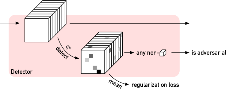
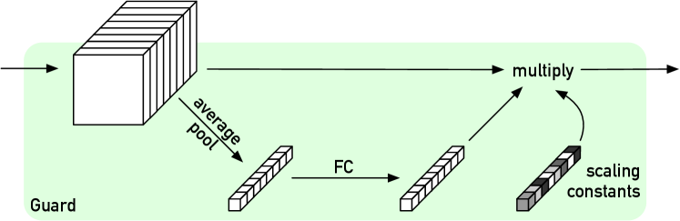
We start with a high-level description of our method. Each convolutional layer with ReLU activation is sequentially extended with a guard (Figure 1(b)) and a detector (Figure 1(a)) layer. Intuitively, the guard encourages the gradient to disperse among differently initialized models, limiting sample transferability. If this fails, the detector works as our second line of defence by raising an alarm at potentially adversarial samples. The rest of this section explains the design of the two modules, which work in tandem or individually to defend against and/or detect most instances of the adversarial attacks considered here.

(a) Detector.

(b) Guard.

Figure 1: High-level view of the module extensions we add to networks to stop and detect transferred adversarial samples.

3.2 Static Channel Manipulation

Where an attack sample is transferable, we hypothesize that by moving along the gradient direction of the input image that gave rise to the adversarial sample, some of the neurons of the network are likely to be highly excited. By monitoring abnormal excitation, we can detect many adversarial samples.

In Sitatapatra, we use a simple concept – we train neural networks using the original datasets, but with additional activation regularization, so that a certain set of outputs, and of intermediate activation values, are not generated by any of the training set inputs. If one of these ‘taboo’ activations is observed, this serves as a signal that the input may be adversarial. As different instances of the model can be trained with different taboo sets, we have a way to introduce diversity that is analogous to the keys used in cryptographic systems. This approach is much faster than, for example, adversarial training [9]. By regularizing the activation feature maps, clean samples yield well-bounded activation results, yet adversarial ones typically result in highly excited neuron outputs in activations [32]. Using this, we can design our detector (Figure 1(a)) so that uncompromised models can successfully block most adversarial samples transferred from compromised models, even under the strong assumption that the models share the same network architecture and dataset.

For simplicity, we consider a feed-forward CNN $F$ consisting of a sequence of $L$ convolutional layers, where the ${l}^{\mathrm{th}}$ layer computes output feature maps $\mathbf{x}_{l}\in\mathbb{R}^{C_{l}\times H_{l}\times W_{l}}$. Here, $\mathbf{x}_{l}$ is a collection of feature maps with $C_{l}$ channels of $H_{l}\times W_{l}$ images, where $H_{l}$ and $W_{l}$ respectively denote the width and height of the image.

The detector module additionally performs the following polynomial transformation $f_{k}$ to the features of each layer output, which can be derived from the key of the network:

$$f_{k}(\mathbf{x}_{l})=a_{n}\mathbf{x}_{l}^{n}+a_{n-1}\mathbf{x}^{n-1}+\cdots+a_{0},$$ (3)

and the transformation is then followed by the following criterion evaluation:

$$g_{k}(\mathbf{x}_{l})=f_{k}\left(\mathbf{x}_{l}\right)\cdot{\left(\mathrm{sign}\left(f_{k}\left(\mathbf{x}_{l}\right)-t\right)\right)}_{+}.$$ (4)

Here, $\cdot$ is element-wise multiplication, ${(\mathbf{z})}_{+}=\max(0,\mathbf{z})$ denotes the ReLU activation, the degrees of the polynomial $n$ and the constant values $a_{0}$, $a_{1}$, …, $a_{n}$ and $t>0$ can be identified as the key embedded into the network. During training with clean dataset samples, any values $f_{k}(\mathbf{x}_{l})>t$ are penalized, with the following regularization term:

$$\mathcal{R}(\mathbf{x})=\sum_{l\in L}{\left\|g_{k}\left(\mathbf{x}_{l}\right)\right\|}_{1}.$$ (5)

As we will examine closely in Section 4, the $g_{k}(\mathbf{x}_{l})$ evaluated from adversarial samples generally produce positive results, whereas clean validation samples usually do not trigger this criterion. Our detector uses this to identify adversarial samples. In addition, the polynomial can be evaluated efficiently with Horner’s method [15], requiring only $n$ multiply-accumulate operations per value, which is insignificant when compared to the computational cost of the convolutions. Finally, the non-linear nature of our regularization diversifies the weight distributions among models, which intuitively explains why adversarial samples become less likely to transfer.

3.3 Dynamic Channel Manipulation

In this section, we present the design of the guard module. It dynamically manipulates feature maps using per-channel attention, which is in turn inspired by the squeeze-excitation networks [11] and feature boosting [8]. As with the detector modules described earlier in Section 3.2, we extend existing networks by adding a guard module immediately after each convolutional layer and its detector module. The ${l}^{\mathrm{th}}$ module accepts $\mathbf{x}_{l}$ computed by the previous convolutional layer as its input, and introduces a small auxiliary network $h:\mathbb{R}^{C_{l}\times H_{l}\times W_{l}}\to\mathbb{R}^{C_{l}\times H_{l}\times W_{l}}$, which amplifies important channels and suppresses unimportant ones in feature maps, before feeding the results of $h(\mathbf{x}_{l})$ to the next convolutional layer. The auxiliary network is illustrated in Figure 1(b) and is defined as:

$$h(\mathbf{x}_{l})=\mathbf{x}_{l}\cdot\left(\bm{\gamma}_{l}\cdot\mathrm{pool}\left(\mathbf{x}_{l}\right)\bm{\phi}_{l}\right),$$ (6)

where $\mathrm{pool}:\mathbb{R}^{C_{l}\times H_{l}\times W_{l}}\to\mathbb{R}^{C_{l}}$ performs a global average pool on the feature maps $\mathbf{x}_{l}$ which reduces them to a vector of $C_{l}$ values, $\bm{\phi}\in\mathbb{R}^{C_{l}\times C_{l}}$ is a matrix of trainable parameters, and $\cdot$ denotes element-wise multiplication between tensors which broadcasts in a channel-wise manner. Finally, $\bm{\gamma}_{l}$ is a vector of $C_{l}$ scaling constants, where each value is randomly drawn from a uniform distribution between 0 and 1, using the crypto-key embedded within the model as the random seed. By doing so, each deployed model can have a different $\bm{\gamma}_{l}$ value, which diversifies the gradients among models and forces the fine-tuned models to adopt different local minima.

4 Evaluation

4.1 Networks, Datasets and Attacks

We evaluate Sitatapatra on two datasets: MNIST [19], CIFAR10 [16]. In MNIST, we use the LeNet5 architecture [20]. In CIFAR10, we use an efficient CNN architecture (MCifarNet) from Mayo [36] that achieved a high classification rate using only 1.3M parameters. ResNet18 is also considered on the CIFAR10 dataset [10].

We evaluated the performance of clean networks and Sitatapatra networks, using two clean models with different initializations as the baseline. For the Sitatapatra models we had two different keys applied on the source and target models. The keys used are $2x^{2}+3x+5<6$ and $0.1x^{2}-x+2<3$ respectively. Throughout the development of Sitatapatra we have tried using a large number of different keys and observed that the performance of the detector is largely dependant on the strictness of the regulariser. For evaluation purposes we have decided to report on the worst performance, practically showing the detection lower bound. The relative performance of other keys will be presented later in Section 5. We consider attacks listed in Section 2 in White and Black-box settings. For the latter, we estimate gradients using a simple coordinate-wise finite difference method [12].

4.2 Static and Dynamic Channel Manipulations

LeNet5 MCifarNet ResNet18-Cifar10 Params $S_{\mathsf{Acc}}(\%)$ $T_{\mathsf{Acc}}(\%)$ $\Delta_{\mathsf{Acc}}(\%)$ $T_{\mathsf{Det}}(\%)$ $l_{2}$ $l_{\infty}$ $S_{\mathsf{Acc}}(\%)$ $T_{\mathsf{Acc}}(\%)$ $\Delta_{\mathsf{Acc}}(\%)$ $T_{\mathsf{Det}}(\%)$ $l_{2}$ $l_{\infty}$ $S_{\mathsf{Acc}}(\%)$ $T_{\mathsf{Acc}}(\%)$ $\Delta_{\mathsf{Acc}}(\%)$ $T_{\mathsf{Det}}(\%)$ $l_{2}$ $l_{\infty}$ Clean 99.13 99.25 - - - - 89.51 90.14 - - - - 91.12 93.58 - - - - FGSM $\epsilon=0.02$ 97.30 98.44 1.14 0.00 0.43 0.02 26.42 38.64 12.22 1.85 1.00 0.02 39.29 59.41 20.12 1.15 1.03 0.02 $\epsilon=0.05$ 92.19 97.44 5.26 0.00 1.07 0.05 22.87 32.95 10.09 1.53 2.43 0.04 30.18 44.74 14.56 0.75 2.50 0.05 $\epsilon=0.1$ 80.11 95.45 15.34 0.00 2.13 0.10 16.48 25.00 8.52 3.17 4.63 0.09 19.28 30.41 11.13 20.10 4.84 0.09 $\epsilon=0.15$ 63.07 90.06 26.99 0.00 3.18 0.15 9.23 17.47 8.24 18.11 6.84 0.13 11.51 24.01 12.50 93.02 7.12 0.13 $\epsilon=0.35$ 6.68 30.54 23.86 0.00 7.31 0.35 1.14 14.20 13.07 86.29 14.61 0.29 3.51 13.57 10.06 91.69 15.21 0.30 FGSM /w GE $\epsilon=0.02$ 97.87 99.15 1.28 0.00 0.43 0.02 28.41 39.35 10.94 2.03 0.97 0.02 40.91 60.94 20.03 1.68 1.03 0.02 $\epsilon=0.05$ 95.31 98.44 3.12 0.00 1.07 0.05 25.28 35.65 10.37 2.09 2.38 0.04 29.69 44.32 14.63 0.25 2.50 0.05 $\epsilon=0.1$ 82.39 96.31 13.92 0.00 2.14 0.10 18.04 26.56 8.52 3.28 4.47 0.08 18.32 29.40 11.08 17.63 4.88 0.09 $\epsilon=0.15$ 62.93 92.61 29.69 0.00 3.19 0.15 11.22 19.32 8.10 17.24 6.54 0.12 9.94 23.44 13.49 93.85 7.17 0.13 $\epsilon=0.35$ 7.67 32.10 24.43 0.00 7.35 0.35 1.42 15.48 14.06 84.84 14.21 0.28 2.70 14.63 11.93 91.86 15.27 0.30 PGD $i=10$ 64.63 98.44 33.81 0.00 1.57 0.09 1.14 41.90 40.77 1.84 0.76 0.02 12.12 61.09 48.97 0.30 0.82 0.03 $i=20$ 0.85 98.44 97.59 0.00 1.96 0.12 0.28 41.90 41.62 1.84 0.76 0.02 10.40 61.09 50.69 0.30 0.90 0.04 $i=50$ 0.00 98.44 98.44 0.00 1.96 0.12 0.00 41.90 41.90 1.84 0.76 0.02 7.43 60.94 53.51 0.29 1.03 0.05 PGD /w GE $i=10$ 65.06 98.72 33.66 0.00 1.61 0.09 0.99 43.61 42.61 1.89 0.76 0.02 13.21 63.21 50.00 1.04 0.83 0.03 $i=20$ 0.85 98.72 97.87 0.00 1.99 0.12 0.28 43.61 43.32 1.89 0.76 0.02 11.22 63.21 51.99 1.04 0.92 0.04 $i=50$ 0.00 98.72 98.72 0.00 2.00 0.12 0.00 43.61 43.61 1.89 0.76 0.02 8.24 63.07 54.83 1.04 1.06 0.05 DeepFool $i=50$ 11.48 98.91 87.42 0.00 1.51 0.39 0.23 76.25 76.02 1.30 0.38 0.05 3.75 77.27 73.52 7.63 0.87 0.10 $i=10$ 89.61 99.22 9.61 0.00 1.44 0.37 2.97 76.17 73.20 1.30 0.38 0.05 6.33 77.50 71.17 6.95 0.81 0.10 C&W $lr=0.5$ 4.38 93.98 89.61 2.35 2.95 0.66 3.83 11.48 7.66 67.41 9.82 0.25 2.73 20.55 17.81 95.50 10.11 0.25 $lr=1.0$ 1.56 80.47 78.91 4.78 3.74 0.75 5.31 13.91 8.59 92.02 17.11 0.43 3.52 11.72 8.20 96.05 17.84 0.46 C&W $lr=0.5$ 4.61 29.92 25.31 16.02 5.22 0.94 4.53 4.77 0.23 99.10 17.37 0.61 3.05 15.70 12.66 98.60 12.63 0.38 $c=0.999$ $lr=1.0$ 1.88 14.53 12.66 24.07 5.92 0.98 7.19 7.58 0.39 100.00 23.58 0.80 5.55 8.67 3.12 98.72 22.20 0.72

Table 2: Transferability of different models on various datasets with the SDCM instrumentation (Guard and Detector). Source and Target are two models of the same topology but different SDCM instrumentations. We generate adversarial samples from source models and apply them on the target models. $S_{\mathsf{Acc}}$ and $T_{\mathsf{Acc}}$ are the accuracies on source and target models. $T_{\mathsf{Det}}$ is the detection ratio on the targeting model. $l_{2}$ and $l_{\infty}$ are the norm values of the adversarial noise, larger norm values mean larger perturbations. $\epsilon$ is a hyperparameter in FGSM, $i$ is the number of iterations and $lr$ is the learning rate. $c$ is the confidence, the adversarial sample has to cause the misclassified class to have a probability above this given threshold. ‘w/ GE’ indicates attacks that use numerical gradient estimation, and they are only reported on MCifarNet because of their long run-time nature.

Table 2 shows the performance of combined static and dynamic channels manipulation (SDCM) method. During the training phase we tune each model to have less than $1\%$ false positive detection rate on the clean evaluation dataset. The results show good performance on large models, since large models have more channels available for the proposed instrumentations. For ResNet18 on CIFAR10, we can achieve above $95\%$ detection of all adversarial samples. Similarly, we believe that the performance increase, in comparison to both LeNet5 and MCifarNet, comes from an increased number of channels of the ResNet18 model. Furthermore, we observe a trade-off between the accuracy difference ($\Delta_{\mathsf{acc}}$) and the detection rate ($T_{\mathsf{det}}$). When attacks achieve low classification accuracies on the target model, the detector, acting as a second line of defence, usually identifies the adversarial examples.

Further, it can be noticed that the samples that actually transfer well usually result in relatively larger distortions — e.g. C&W with high confidence and FGSM $0.6$. Although large distortions allow attacks to trick the models, they inevitably trigger the alarm and thus get detected. Meanwhile, attacks with more fine-grained perturbations fail to transfer and the accuracy $T_{\mathsf{acc}}$ remains high. For example, DeepFool consistently shows high $T_{\mathsf{acc}}$ and high $\Delta_{\mathsf{acc}}$.

Pretrained Static Only Combined $\Delta_{\mathsf{Acc}}(\%)$ $\Delta_{\mathsf{Acc}}(\%)$ $T_{\mathsf{Det}}(\%)$ $\Delta_{\mathsf{Acc}}(\%)$ $T_{\mathsf{Det}}(\%)$ FGSM $\epsilon=0.02$ 0.70 1.87 0.00 0.94 0.00 $\epsilon=0.08$ 3.98 15.78 0.00 9.14 0.00 $\epsilon=0.6$ 3.05 10.78 0.19 11.02 22.28 DeepFool $i=50$ 77.11 78.20 0.00 87.42 0.00 $i=10$ 9.22 1.02 0.00 9.61 0.00 C&W $lr=0.5$ 82.81 91.02 0.00 89.61 2.35 $lr=1.0$ 59.84 90.39 0.95 78.91 4.78 $c=0.999$ $lr=0.5$ 11.88 57.50 2.38 25.31 16.02 $lr=1.0$ 5.08 45.00 6.47 12.66 24.07

Table 3: Transferability of LeNet5 on MNIST with different instrumentations. $\Delta_{\mathsf{acc}}$ is the difference in accuracies and $T_{\mathsf{det}}$ is the detection rate. $l_{2}$ and $l_{\infty}$ are the averaged $l_{2}$ and $l_{\infty}$ norms of the distortions on all input images. $\epsilon$ is a hyperparameter in FGSM, $i$ is the number of steps and $lr$ is learning rate. $c$ is the confidence, the adversarial sample has to cause the misclassified class to have a probability above this given threshold. We use $20$ steps on C&W.

Finally, to demonstrate the overall performance of Sitatapatra, we present a comparison between the baseline, SCM and SDCM in Table 3. Both of the proposed methods perform relatively worse for LeNet5 , as mentioned before, we believe that this due to the small number of channels at its disposal. Having said that, the proposed methods still greatly outperforms the baseline in terms of $\Delta_{\mathsf{acc}}$. The results of DeepFool are very similar across all three methods. DeepFool was not designed with transferability in mind. In contrast, C&W was previously shown to generate highly transferable adversarial samples. The combined method manages to successfully classify the transferred samples and shows sensible detection rates.

5 Discussion

5.1 Accuracy, Detection and Computation Overheads

In this section we discuss the trade-offs facing the Sitatapatra user. First and foremost, the choice of keys has an impact on transferability.

(a) Change in Accuracies ($\Delta_{\mathsf{acc}}$).

(b) Detection rates on the target model ($T_{\mathsf{det}}$)

Figure 2: Changes in accuracies and detection rates of LeNet5 with various SDCM instrumentations

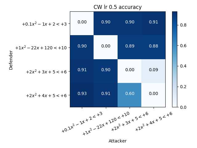
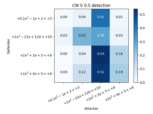
In Figure 2, we present a confusion matrix with differently instrumented LeNet5 networks attacking each other with C&W attack for $20$ steps and a learning rate of $0.5$. The chosen instrumentations are all second-order polynomials, but with different coefficients. It is apparent that Sitatapatra improves the accuracies reported in Figure 2(a). However, for the two polynomials, $2x^{2}+3x+5<6$ and $2x^{2}+4x+5<6$, the behavior is different. When using the adversarial samples from $2x^{2}+4x+5<6$ to attack $2x^{2}+3x+5<6$, there is almost zero change in accuracy between the source and the target model, but this relationship does not hold in reverse. The above phenomenon indicates that the adversarial samples generated from one polynomial are transferable to the other when the polynomials are too similar. The same effect is observed in the detector shown in Figure 2(b): it is easier to detect adversarial samples from $2x^{2}+4x+5<6$ to attack $2x^{2}+3x+5<6$.

This indicates that, when the models get regularized to polynomials that are similar, the attacks between them end up being transferable. Fortunately, the detection rates remain relatively high even in this case. Different polynomials restrict the activation value range in different ways. In practice, we found that the smaller the range that is available , i.e. the unpenalized space for activations, the harder it is to train the network. Intuitively, if the regularization applies too strict a constraint to activation values, the stochastic gradient descent process struggles to converge in a space full of local minima. However, a strong restriction on activation values caused detection rates to improve. Thus, when deploying models with Sitatapatra, the choice of polynomials affects base accuracies, detection rates and training time.

Key choice brings efficiency considerations to the table as well. Although training time for individual devices may be a bearable cost in many applications, a substantial increase in run-time computational cost will often be unacceptable. Figure 4 reflects the total additional costs incurred by using Sitatapatra in our evaluation models. The $<7.5\%$ overhead we add to the base network is small, given that the models demonstrate good defence and detection rates against adversarial samples. It is notable that during inference, a detector module requires for each value $n$ fused multiply-add operations to evaluate a $n$-degree $f_{k}$ polynomial using Horner’s method [15], and $1$ additional operation for threshold comparison, and thus utilize $(n+1)C_{l}H_{l}W_{l}$ operations in total for the ${l}^{\mathrm{th}}$ convolutional layer. In our evaluation, we set $n=2$ by using second-order polynomials. Additionally, a guard module of the ${l}^{\mathrm{th}}$ layer uses channel-wise averaging, a fully connected layer, a channel-wise scaling, and element-wise multiplications for all activations, which respectively require $C_{l}H_{l}W_{l}$, $C_{l}^{2}$, $C_{l}$, and $C_{l}H_{l}W_{l}$ operations.

5.2 Key attribution

While exploring which activations ended up triggering an alarm with different Sitatapatra parameters, we noticed that we could often attribute the adversarial samples to the models used to generate them. In practice, this is a huge benefit, known as traitor tracing in the crypto research community: if somebody notices an attack, she can identify the compromised device and take appropriate action. We conducted a simple experiment to evaluate how to identify the source of a different adversarial sample. We first produced models instrumented with different polynomials using Sitatapatra and then generated the adversarial examples.

In this simple experiment, we use a support vector machine (SVM) to classify the adversarial images based on the models generated them. The SVM gets trained on the 5000 adversarial samples and gets tested on a set of 10000 unseen adversarial images. The training and test sets are disjoint.

Model #FLOPs original detector guard total overhead LeNet5 480,500 28,160 7,660 516,320 7.45% ResNet18 37,016,576 152,094 1,847,106 39,015,776 5.40% MCifarNet 174,301,824 715,422 646,082 175,663,328 0.64%

Figure 3: The computational costs, measured in the number of FLOPs, added by the detector and guard modules to the original network.

FGSM FGSM+DeepFool+C&W Polynomial Precision Recall F1 Precision Recall F1 $0.1x^{2}-1x+2<3$ 0.90 0.90 0.90 0.81 0.29 0.43 $x^{2}-22x+120<10$ 0.90 0.89 0.90 0.85 0.28 0.42 $2x^{2}+3x+5<6$ 0.53 0.72 0.61 0.34 0.33 0.33 $2x^{2}+4x+5<6$ 0.56 0.35 0.43 0.30 0.69 0.41 Micro F1 0.72 0.72 0.72 0.40 0.40 0.40 Macro F1 0.72 0.72 0.71 0.57 0.40 0.40

Figure 4: Key attribution based on the adversarial sample produced.

Figure 4 shows the classification results for FGSM-generated samples and all attacks combined. Precision, Recall and F1 scores are reported. In addition, we report the micro and macro aggregate values of F1 scores – micro counts the total true positive, false negatives and false positives globally, whereas macro takes label imbalance into account.

For both scenarios, we get a performance that is much better than random guessing. First, it is easier to attribute adversarial samples generated by the large coarse-grained attacks. Second, for polynomials that are different enough, the classification precision is high – for just FGSM we get a $90\%$ recognition rate, while with more attacks it falls to $81\%$ and $85\%$. For similar polynomials, we get worse performance, of around $50\%$ for FGSM and around $30\%$ for all combined.

This bring an additional trade-off – training a lot of different polynomials is hard, but it allows easier identification of adversarial samples. This then raises the question of scalability of the Sitatapatra model instrumentation.

5.3 Key size

In 1883, the cryptographer Auguste Kerckhoffs enunciated a design principle that is used today: a system should withstand enemy capture, and in particular it should remain secure if everything about it, except the value of a key, becomes public knowledge [14]. Sitatapatra follows this principle – as long as the key is secured, it will, at a minimal cost, provide an efficient way to protect against low-cost attacks at scale. The only difference is that if an opponent secures access to a system protected with Sitatapatra, then by observing its inputs and outputs he can use standard optimisation methods to construct adversarial samples. However these samples will no longer transfer to a system with a different key. One of the reasons why sample transferability is an unsolved problem is because it has so far been hard to generate a wide enough variety of models with enough difference between them at scale.

Sitatapatra is the first attempt at this problem, and it shows possibilities to embed different polynomial functions as keys to CNNs to block transfer of adversarial samples. Modern networks have hundreds of layers and channels, and thus can embed different keys at various parts improving key diversity. The potential implication of having a key is important. In the case where a camera vendor wants to sell the same vision system to banks as in the mass market, it may be sufficient to have a completely independent key for the cameras sold to each bank. It will also be sensible for a mass-market vendor wants to train its devices in perhaps several dozen different families, in order to stop attacks scaling (a technique adopted by some makers of pay-TV smartcards [1]). However it would not be practical to have an individual key for each unit sold for a few dollars in a mass market. The fact that adding keys to neural networks can improve its diversity solves the problem of training multiple individual neural networks on the same dataset, which is also known as a model ensemble. In fact, our key instrumentation and the model identification from a model ensemble together can be seen as a stream of deployment, which also sufficiently increases the key space.

6 Conclusion

In this paper we presented Sitatapatra, a new way to use both static and dynamic channel manipulations to stop adversarial sample transfer. We show how to equip models with guards that diffuse gradients and detectors that restrict their ranges, and demonstrate the performance of this combination on CNNs of varying sizes. The detectors enable us to introduce key material as in cryptography so that adversarial samples generated on a network with one key will not transfer to a network with a different one, as activations will exceed the ranges ranges permitted by the detectors and set off an alarm. We described the trade-offs in terms of accuracy, detection rate, and the computational overhead both for training and at run-time. The latter is about five percent, enabling Sitatapatra to work on constrained devices. The real additional cost is in training but in many applications this is perfectly acceptable. Finally, with a proper choice of transfer functions, Sitatapatra also allows adversarial sample attribution, or ‘traitor tracing’ as cryptographers call it – so that a compromised device can be identified and dealt with.

References

- [1] R. Anderson. Security engineering: a guide to building dependable distributed systems. 2008.
- [2] S. Antol, A. Agrawal, J. Lu, M. Mitchell, D. Batra, C. Lawrence Zitnick, and D. Parikh. Vqa: Visual question answering. In Proceedings of the IEEE international conference on computer vision, pages 2425–2433, 2015.
- [3] V. Badrinarayanan, A. Kendall, and R. Cipolla. Segnet: A deep convolutional encoder-decoder architecture for image segmentation. arXiv preprint arXiv:1511.00561, 2015.
- [4] N. Carlini, P. Mishra, T. Vaidya, Y. Zhang, M. Sherr, C. Shields, D. Wagner, and W. Zhou. Hidden Voice Commands. In 25th USENIX Security Symposium (USENIX Security 16). USENIX Association, 2016.
- [5] N. Carlini and D. Wagner. Towards Evaluating the Robustness of Neural Networks. In 2017 IEEE Symposium on Security and Privacy (SP), pages 39–57. IEEE, 2017.
- [6] K. Eykholt, I. Evtimov, E. Fernandes, B. Li, A. Rahmati, C. Xiao, A. Prakash, T. Kohno, and D. Song. Robust Physical-World Attacks on Deep Learning Visual Classification. In Proceedings of the IEEE Conference on Computer Vision and Pattern Recognition, pages 1625–1634, 2018.
- [7] C.-Y. Fang, S.-W. Chen, and C.-S. Fuh. Road-sign detection and tracking. IEEE transactions on vehicular technology, 52(5):1329–1341, 2003.
- [8] X. Gao, Y. Zhao, L. Dudziak, R. Mullins, and C. zhong Xu. Dynamic channel pruning: Feature boosting and suppression. In International Conference on Learning Representations, 2019.
- [9] I. J. Goodfellow, J. Shlens, and C. Szegedy. Explaining and harnessing adversarial examples. International Conference on Learning Representations (ICLR), 2015.
- [10] K. He, X. Zhang, S. Ren, and J. Sun. Deep residual learning for image recognition. In Proceedings of the IEEE conference on computer vision and pattern recognition, pages 770–778, 2016.
- [11] J. Hu, L. Shen, and G. Sun. Squeeze-and-excitation networks. arXiv preprint arXiv:1709.01507, 7, 2017.
- [12] A. Ilyas, A. Jalal, E. Asteri, C. Daskalakis, and A. G. Dimakis. The robust manifold defense: Adversarial training using generative models.
- [13] S. Ji, W. Xu, M. Yang, and K. Yu. 3d convolutional neural networks for human action recognition. IEEE transactions on pattern analysis and machine intelligence, 35(1):221–231, 2013.
- [14] A. Kerckhoffs. La cryptographie militaire. pages 161–191, 1883.
- [15] D. E. Knuth. Evaluation of polynomials by computer. Communications of the ACM, 5(12):595–599, 1962.
- [16] A. Krizhevsky, V. Nair, and G. Hinton. The CIFAR-10 dataset. 2014.
- [17] A. Krizhevsky, I. Sutskever, and G. E. Hinton. ImageNet classification with deep convolutional neural networks. In Advances in neural information processing systems, pages 1097–1105, 2012.
- [18] A. Kurakin, I. Goodfellow, and S. Bengio. Adversarial examples in the physical world. arXiv preprint arXiv:1607.02533, 2016.
- [19] Y. LeCun, C. Cortes, and C. Burges. MNIST handwritten digit database. 2, 2010.
- [20] Y. LeCun et al. LeNet-5, convolutional neural networks. page 20, 2015.
- [21] X. Liu, M. Cheng, H. Zhang, and C.-J. Hsieh. Towards robust neural networks via random self-ensemble. In European Conference on Computer Vision, pages 381–397, 2018.
- [22] X. Liu, Y. Li, C. Wu, and C.-J. Hsieh. Adv-BNN: Improved Adversarial Defense through Robust Bayesian Neural Network. In International Conference on Learning Representations, 2019.
- [23] Y. Liu, X. Chen, C. Liu, and D. Song. Delving into transferable adversarial examples and black-box attacks. In International Conference on Learning Representations (ICLR), 2017.
- [24] D. Meng and H. Chen. Magnet: A two-pronged defense against adversarial examples. In Proceedings of the 2017 ACM SIGSAC Conference on Computer and Communications Security, CCS ’17, pages 135–147, New York, NY, USA, 2017. ACM.
- [25] J. H. Metzen, T. Genewein, V. Fischer, and B. Bischoff. On detecting adversarial perturbations. In Proceedings of 5th International Conference on Learning Representations (ICLR), 2017.
- [26] S. Moosavi-Dezfooli, A. Fawzi, and P. Frossard. DeepFool: a simple and accurate method to fool deep neural networks. 2016.
- [27] N. Papernot, P. McDaniel, and I. Goodfellow. Transferability in machine learning: from phenomena to black-box attacks using adversarial samples. arXiv preprint, 2016.
- [28] N. Papernot, P. McDaniel, I. Goodfellow, S. Jha, Z. B. Celik, and A. Swami. Practical black-box attacks against machine learning. pages 506–519, 2017.
- [29] N. Papernot, P. McDaniel, X. Wu, S. Jha, and A. Swami. Distillation as a defense to adversarial perturbations against deep neural networks. 2016 IEEE Symposium on Security and Privacy (SP), May 2016.
- [30] S. Ren, K. He, R. Girshick, and J. Sun. Faster R-CNN: Towards real-time object detection with region proposal networks. In Advances in neural information processing systems, pages 91–99, 2015.
- [31] F. Schroff, D. Kalenichenko, and J. Philbin. Facenet: A unified embedding for face recognition and clustering. In Proceedings of the IEEE conference on computer vision and pattern recognition, pages 815–823, 2015.
- [32] I. Shumailov, Y. Zhao, R. Mullins, and R. Anderson. The taboo trap: Behavioural detection of adversarial samples. arXiv preprint arXiv:1811.07375, 2018.
- [33] C. Szegedy, W. Zaremba, I. Sutskever, J. Bruna, D. Erhan, I. J. Goodfellow, and R. Fergus. Intriguing properties of neural networks. CoRR, abs/1312.6199, 2013.
- [34] D. Tsipras, S. Santurkar, L. Engstrom, A. Turner, and A. Madry. Robustness may be at odds with accuracy. In International Conference on Learning Representations, 2019.
- [35] Z. Yan, Y. Guo, and C. Zhang. Deep defense: Training dnns with improved adversarial robustness. In S. Bengio, H. Wallach, H. Larochelle, K. Grauman, N. Cesa-Bianchi, and R. Garnett, editors, Advances in Neural Information Processing Systems 31, pages 417–426. 2018.
- [36] Y. Zhao, X. Gao, R. Mullins, and C. Xu. Mayo: A framework for auto-generating hardware friendly deep neural networks. 2018.
- [37] Y. Zhao, I. Shumailov, R. Mullins, and R. Anderson. To compress or not to compress: Understanding the interactions between adversarial attacks and neural network compression. arXiv preprint arXiv:1810.00208, 2018.