A discontinuity in the $T_{\rm eff}$-radius relation of M-dwarfs

Abstract

We report on 13 new high-precision measurements of stellar diameters for low-mass dwarfs obtained by means of near-infrared  long-baseline interferometry with PIONIER at the Very Large Telescope Interferometer. Together with accurate parallaxes from Gaia DR2, these measurements provide precise estimates for their linear radii, effective temperatures, masses, and luminosities. This allows us to refine the effective temperature scale, in particular towards the coolest M-dwarfs. We measure for late-type stars with enhanced metallicity slightly inflated radii, whereas for stars with decreased metallicity we measure smaller radii. We further show that Gaia DR2 effective temperatures for M-dwarfs are underestimated by $\sim$ 8.2% and give an empirical $M_{G}$-$T_{\rm eff}$ relation which is better suited for M-dwarfs with $T_{\rm eff}$ between 2600 and 4000 K. Most importantly, we are able to observationally identify a discontinuity in the $T_{\rm eff}$-radius plane, which is likely due to the transition from partially convective M-dwarfs  to the fully convective regime. We found this transition to happen between 3200 K and 3340 K, or equivalently for stars with masses $\approx 0.23\,M_{\sun}$. We find that in this transition region the stellar radii are in the range from 0.18 to 0.42 $R_{\sun}$ for similar stellar effective temperatures.

1 Introduction

Low-mass dwarfs are the most numerous stars in the Universe, and understanding them is thus clearly an important endeavour. Beyond their own interest, investigations by Bonfils et al. (2013), Dressing & Charbonneau (2013) and Kopparapu (2013) have shown that M-dwarfs  may be the most abundant planet hosts in the Milky Way as well. The estimation of parameters and properties of an exoplanet are intimately connected to the stellar host, e.g. the stellar mass determines the measured semi-amplitude for radial velocity observations and hence influences the mass estimate of the planet. In the case of transiting extrasolar planets (TEPs), their physical radii can be measured from the transit shape if the radii of the stellar hosts are known. In addition, the stellar radius and effective temperature are linked to the planet’s surface temperature and the location of the habitable zone. All of these examples illustrate how important stellar astrophysical properties are for the characterization of exoplanets in general. M-dwarfs are attractive targets to search for transiting exoplanets not only due to their numbers, but also due to the fact that for a given planetary size the transit depth is deeper around low-mass stars due to their smaller sizes. Also, the habitable zone around these stars is closer, resulting in shorter periods that make detection easier. Indeed, one of the main drivers for the upcoming TESS mission (Ricker et al., 2014) is to detect transiting exoplanets around low-mass stars.

A fundamental stellar property is the radius, and for low-mass stars its estimation has been done mostly through stellar models. Fortunately, considerable improvements in interferometric observation techniques allow us now to obtain stellar parameters such as the stellar radius directly. However, these measurements become more difficult as we go to cooler dwarf stars due to their inherently lower luminosity and smaller radii. Measured angular diameters of M-dwarfs are generally close to the current baseline limit of available interferometers. Up to now, extensive interferometric observations on M-dwarf stars have been done mainly from the Northern Hemisphere with the CHARA array (Berger et al., 2006; von Braun et al., 2011; Boyajian et al., 2012a; von Braun et al., 2014) and a few with the VLT-Interferometer (VLTI) from the South (Ségransan et al., 2003; Demory et al., 2009). These interferometric direct measurements showed a discrepancy with the parameters measured indirectly (Boyajian et al., 2012b). The work of Boyajian et al. (2012b) found in particular large disagreements for low-mass stars, where the radii measured by interferometers were more than 10% larger than the ones based on models from Chabrier & Baraffe (1997). Likewise, Kesseli et al. (2018) found that this inflation of the M-dwarf radii extends down to the fully convective regime with a discrepancy of 13% – 18%.

This discrepancy affects in turn other stellar parameters like surface temperature ($T_{\rm eff}$), gravities ($\log{g}$), masses, luminosities, and eventually also possible planetary parameters. Therefore, it is important to observe and re-evaluate the properties of more M-dwarf  stars with interferometric observations, particularly towards the later spectral types which have not been extensively studied at all.

Theoretical stellar evolution models for low-mass stars predict a transition into the fully convective regime to occur somewhere between 0.2 $M_{\sun}$ (Dorman et al., 1989) and 0.35 $M_{\sun}$ (Chabrier & Baraffe, 1997), depending on the underlying stellar model. For partially convective stars, the stellar structure is Sun-like, having a radiative zone and a convective envelope. The only previous observational indications for this transition in late-type stars are based on observations of magnetic fields and measurements of stellar rotational periods. Browning (2008) showed that stars whose convective region extends to the core have strong large-scale magnetic fields and, in fact, we have observational evidence that the fraction of M-dwarfs with strong magnetic fields on a large scale is higher for mid- to late-type M-dwarfs than for early type ones (Donati et al., 2008). On the other hand, Wright & Drake (2016) showed that rotation-dependent dynamos are very similar in both partially and fully convective stars. Irwin et al. (2011) and Newton et al. (2016) measured rotational spin-velocities of M-stars. The authors found two divergent populations of faster and slower rotators in the fully convective mass regime, which makes rotation measurements difficult to use in the determination of whether a late-type star is fully convective. Moreover, the rotation of fully convective stars depends on both age and mass. All former indications of fully convective stars have been done indirectly and are not unambiguous.

In this work we present directly measured physical parameters for a sample of 13 low-mass stars using observations with the VLT-Interferometer (VLTI). These observations are used to probe the transition between the partially and fully convective regimes and to identify the dependence of the stellar radii on other stellar properties. The paper is structured as follows. In §2 we lay out the observational details. In §3 we detail how we estimated the stellar physical parameters. Finally, we discuss the implication of the measured stellar parameters on stellar evolution and structure models in §4 and we conclude in §5.

2 Observations and Data Reduction

2.1 PIONIER observations

Our target sample is compiled from a list of M-dwarfs within $\sim 15$ pc (so the stars are resolved within the given VLTI baseline) and with H-band magnitudes $<7$ (so that fringes will be easily visible and we can obtain a good signal-to-noise ratio).

In order to measure the angular diameter of our sample stars, we used the VLTI/PIONIER interferometer (Le Bouquin et al., 2011). PIONIER is an integrated optics four-beam combiner operating at the near-infrared wavelength range. We used the auxiliary telescopes (ATs) in a A1-G1-K0-J3 quadruplet configuration. This configuration gave us the longest VLTI baseline available (from 57 meters between the stations K0 and J3, up to 140 metres between A1 and J3) and we used the Earth’s rotation to further fill the $(u,v)$ plane.

We observed our sample with a three-channel spectral dispersion (SMALL mode), whenever possible. In cases where this was not possible, due to low coherence time on a given night or the relative faintness of the target, we observed without spectral dispersion (FREE mode). Similarly, the number of scan steps were adjusted according to the objects’ brightness and atmospheric conditions. As our sample stars were not too bright we were able to use the fast Fowler readout mode for all of our observations.

Our observing strategy was to bracket each science frame (SCI) with a calibrator star (CAL), observed with the same setup as the science object. The calibrators are chosen to be mostly point-like nearly unresolved stars (van Belle & van Belle, 2005), so the uncertainties in their diameter will not influence our targets, but we also included calibrators with known diameter for verification proposes. We also made sure that the visibility precision of our calibrators was below 1%. In order to search for suitable calibrators, we used the ASPRO2-tool and SearchCal. For each science target we repeated around 11 times a CAL-SCI-CAL block, and in each block we used different calibrator stars. The same target was also observed on different nights. This strategy helped us to beat down the systematic noise from the instrument and atmosphere. We reduced our observed raw fringes to calibrated visibilities and closure phases with a modified version of the PIONIER data reduction software (pndrs, described in Lachaume et al., 2019).

2.2 Calibrated Visibilities and Angular diameters

Our modified data reduction with pndrs is fully described in detail in a publication by Lachaume et al. (2019), where we also show a rigorous analysis of the interferometric measurement errors. Here we will give only a brief summary of the data reduction process and we refer interested readers to Lachaume et al. (2019), for more details on the data analysis. In the first step we calibrate the detector frames. This was done by dark correcting the detector data and from the kappa-matrix we calibrated the transmission of the respective baseline. Finally, we used frames illuminated by an internal light source to calibrate the wavelength. Basically, these calibrated frames will allow us to obtain the raw visibilities, which are in turn the product of true visibilities and the system transfer function. The system transfer function characterizes the response of the interferometer as a function of spatial frequency and in order to get the true visibilities it needs to be estimated by using calibrator stars. Assuming that all our calibrator stars have well known true visibilities, i.e. an unresolved calibrator has a known visibility of unity and a resolved star has a known diameter, either measured or from spectral typing. By further assuming a smooth transfer function, in theory this would allow us to calibrate our raw visibilities. Nevertheless, uncertainties in the assumed calibrators’ diameters can impact all observations in a sequence due to systematic errors in the transfer function estimate (Lachaume et al., 2019, and references therein). Further errors can be introduced through systematic uncertainties in the absolute wavelength calibration (Gallenne et al., 2018) and by several other random effects which will affect the different spectral channels in a similar or imbalanced manner, like e.g. atmospheric jitter or flux variations between the arms of the interferometer. In order to account for the correlation effects in our observations we apply a bootstrap method as described in Lachaume et al. (2019); Lachaume et al. (2014).

Generally, in a bootstrap one resamples several times new data sets from the empirical data itself by replacing parts of the original data. For each candidate, we started by picking randomly interferograms out of the parent population of $\sim 10^{2}$ interferograms. These interferograms are reduced and averaged to a single data set, which corresponds to the raw visibility. As mentioned before, uncertainties in the calibrators’ diameter can cause correlated errors. Therefore, we choose arbitrarily a calibrator with a diameter, drawn randomly from a Gaussian distribution centered on the catalogued diameter and with a width corresponding to the error bars. We used 6 to 18 data sets and calibrators to replace the original data and to calculate the system transfer function and calibrated visibilities. We repeat this procedure to obtain 5,000 bootstrap realizations. These calibrated visibilities were fitted with a uniform disk ($\theta_{\rm UD}$) model to obtain a distribution of angular diameters for each star observed. In Fig. 1 we compare some of our measured $\theta_{\rm UD}$ with the ones available in the literature. We find a good agreement between our measurements and the literature values.

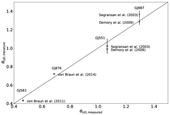
Figure 1: Our angular diameters $\theta_{\rm UD}$  compared to literature values. We find good agreement between our measurements and the literature.

3 Estimating the Physical Parameters from Interferometry

3.1 Calculation of the stellar radius

The limb darkened disk $\theta_{\rm LD}$ is usually obtained by fitting directly a limb darkened disk model to the squared visibilities, assuming a certain limb darkening law and coefficient. Generally, a linear limb darkening law is assumed and tabulated values are used for the coefficients, see e.g. Boyajian et al. (2012b), von Braun et al. (2014), and von Braun et al. (2011). We note, that while $\theta_{\rm UD}$s are independent of stellar models, photospheric diameters, $\theta_{\rm LD}$s depend on stellar models as the limb-darkening coefficient are derived from them. However, the impact on the radius estimate by the limb-darkening in the near-infrared is small (2–4%) and it is mostly dominated by the angular diameter measurement uncertainties and systematics.

In order to estimate the $\theta_{\rm LD}$, we used the $\theta_{\rm UD}$–$\theta_{\rm LD}$ relation from Hanbury Brown et al. (1974):

$$\theta_{\rm LD}(\lambda)=\theta_{\rm UD}\,\sqrt[]{\frac{1-\frac{1}{3}\mu(\lambda,T_{\rm eff},\log{g})}{1-\frac{7}{15}\mu(\lambda,T_{\rm eff},\log{g})}},$$ (1)

where $\theta_{\rm UD}$ is the angular diameter we obtained from the calibrated visibilities and $\mu_{\lambda}$ is the linear limb darkening coefficient as function of wavelength, $T_{\rm eff}$ and $\log{g}$. Rather than using tabulated coefficient, we calculated a grid of limb darkening coefficients following Espinoza & Jordán (2015) corresponding to the atmosphere grid with $T_{\rm eff}$ in range 2300–4500 K, $\log{g}$ in range 4.0–6.0 and a fixed metallicity of 0.0. This allows us to have a conformity with the grid which will be used in Sect. 3.3. As filter transmission function of PIONIER, we used a top hat function between 1.5$\mu{\rm m}$ and 1.8$\mu{\rm m}$.

3.2 $T_{\rm eff}$ estimate

The measured diameters can be related to the effective temperature by

$$T_{\rm eff}=\sqrt[4]{\frac{4F_{\rm bol}}{\sigma\theta_{\rm LD}}},$$ (2)

where $F_{\rm bol}$ is the bolometric flux (obtained by e.g. fitting the spectral energy distribution with literature photometry to spectral templates), $\theta_{\rm LD}$ is the limb darkened angular diameter and $\sigma$ is the Stefan-Boltzmann constant.

3.3 Bolometric flux estimate

In order to estimate the bolometric flux we started by using the PHOENIX atmosphere models from Husser et al. (2013) to create a grid of synthetic photometric points for filters with available photometric observations of our sample stars. Their models are defined in the wavelength range from 0.05 to 5.5$\mu{\rm m}$. Our flux model grid runs $T_{\rm eff}$ from 2300 K to 4500 K, $\log{g}$ between 4.0 and 6.0 dex, and for a fixed metallicity of 0.0 dex. The flux was integrated over the respective band and convolved with the filter profiles from Mann & von Braun (2015). We linearly interpolated this grid of synthetic flux in-between. The bolometric flux $F_{\rm bol}$  of a given star is then defined as:

$$F_{\rm bol}=\int_{0}^{+\infty}F_{\mathrm{model}}(\lambda,T_{\rm eff},\log{g})\frac{R_{\star}^{2}}{d^{2}}\mathrm{d}\lambda,$$ (3)

where $R_{\star}$ is the stellar radius and $d$ is the distance.

3.4 Multinest fitting for $T_{\rm eff}$, $R_{\star}$, and $L_{\star}$

We first collected observed fluxes for our stars using the VizieR photometric query. To these observed fluxes we fitted the model grid using the pymultinest code (Buchner et al., 2014). This program is a python code for multimodal nested sampling technique (Skilling, 2004; Feroz & Hobson, 2008). Our log-likelihood function is

$$\mathcal{\log L}=-\sum_{i=1}^{N_{\mathrm{phot}}}\left[\frac{(F_{i,\mathrm{obs}}-F_{i,\mathrm{mod}})^{2}}{2\sigma_{i}^{2}}-\log{\frac{1}{\sigma_{i}\sqrt{2\pi}}}\right],$$ (4)

where $F_{i,\mathrm{obs}}$ is the observed flux in a given filter $i$, $F_{i,\mathrm{mod}}$ is the synthetic flux in that filter obtained from the atmosphere models, and $\sigma_{i}$ is the corresponding measurement error of the observed flux. The sum goes over the $N_{\mathrm{phot}}$ photometric measurements of a given star.

Our priors are $T_{\rm eff}$, $\log{g}$, distance, and angular diameter $\theta_{\rm UD}$. All our priors were drawn from a normal distribution centered at the literature value and with a dispersion corresponding to the respective error. We further repeated this process using M-dwarfs with measured diameters from von Braun et al. (2012), Boyajian et al. (2012a) and von Braun et al. (2014). Our final parameter estimates are shown in Table 1. We compare our values with the ones from Mann et al. (2015) in Figure 2 and find good agreement with a mean difference of 3% for all three parameters (from top to bottom: radius, $F_{\rm bol}$, $T_{\rm eff}$). In the same Figure 2 (bottom plot), we further compare our effective temperatures with the ones obtained by Neves et al. (2014) through spectral type classification using optical spectroscopy and from Gaia DR2 using Apsis (Andrae et al., 2018). In the latter cases the relative difference for $T_{\rm eff}$ is generally higher, with a mean difference of 5.4% and $-8.2\%$ respectively. Therefore, spectral typing of M-dwarfs in the optical wavelength range generally overestimates $T_{\rm eff}$s, whereas Gaia DR2 $T_{\rm eff}$s are considerably underestimated.

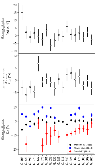
Figure 2: We compare our calculated radius, $F_{\rm bol}$, and $T_{\rm eff}$ with the ones from Mann et al. (2015). Stars are ordered according to our calculated $T_{\rm eff}$ from low (left) to high (right) temperature. The difference between the estimates is small, the mean difference for the radius is 2.9%, $F_{\rm bol}$ is 2.5% and $T_{\rm eff}$ is 1.4%. However, by comparing our $T_{\rm eff}$ with the ones from optical spectroscopy (Neves et al., 2014), we find an higher mean difference of 5.4% and -8.2% for Gaia DR2 $T_{\rm eff}$. However, single $T_{\rm eff}$s from Gaia DR2 can have differences of up to $\sim 15\%$. (See Sect. 3.4 for details)

Table 1: Final parameter estimates obtained through multi-modal nested sampling technique. (See Sect. 3.4 for details)

star	$\theta_{\rm UD}$	$\theta_{\rm LD}$	$\mu_{\lambda}$	$F_{\rm bol}$	$R_{\star}$	parallax	calculated
name	[mas]	[mas]		[$10^{-8}$ $\rm erg\,s^{-1}\,cm^{-2}$]	[$R_{\sun}$]	[mas]	$T_{\rm eff}$[K]
GJ 1	$0.794\pm 0.005$	$0.812\pm 0.005$	0.290	$3.751\pm 0.072$	$0.379\pm 0.002$	$230.133\pm 0.059$	$3616\pm 14$
GJ 273	$0.763\pm 0.010$	$0.783\pm 0.010$	0.335	$2.288\pm 0.118$	$0.320\pm 0.005$	$262.961\pm 1.387$	$3253\pm 39$
GJ 406	$0.562\pm 0.020$	$0.582\pm 0.020$	0.449	$0.563\pm 0.044$	$0.159\pm 0.006$	$394.867\pm 7.893$	$2657\pm 20$
GJ 447	$0.524\pm 0.029$	$0.540\pm 0.029$	0.365	$1.103\pm 0.091$	$0.196\pm 0.010$	$296.309\pm 0.069$	$3264\pm 24$
GJ 551	$1.066\pm 0.007$	$1.103\pm 0.007$	0.422	$2.866\pm 0.210$	$0.154\pm 0.001$	$768.500\pm 0.203$	$2901\pm 68$
GJ 581	$0.464\pm 0.007$	$0.476\pm 0.007$	0.324	$0.967\pm 0.039$	$0.322\pm 0.005$	$158.747\pm 0.051$	$3366\pm 28$
GJ 628	$0.644\pm 0.014$	$0.661\pm 0.014$	0.335	$1.882\pm 0.068$	$0.306\pm 0.007$	$232.209\pm 0.063$	$3372\pm 12$
GJ 674	$0.720\pm 0.037$	$0.737\pm 0.037$	0.318	$2.443\pm 0.232$	$0.360\pm 0.018$	$219.800\pm 0.047$	$3409\pm 25$
GJ 729	$0.625\pm 0.020$	$0.642\pm 0.020$	0.345	$1.370\pm 0.096$	$0.205\pm 0.006$	$336.121\pm 0.064$	$3162\pm 30$
GJ 832	$0.794\pm 0.010$	$0.814\pm 0.010$	0.325	$3.359\pm 0.113$	$0.435\pm 0.005$	$201.407\pm 0.043$	$3512\pm 23$
GJ 876	$0.686\pm 0.009$	$0.705\pm 0.009$	0.342	$1.902\pm 0.058$	$0.354\pm 0.005$	$213.866\pm 0.078$	$3275\pm 18$
GJ 887	$1.297\pm 0.005$	$1.328\pm 0.004$	0.323	$10.916\pm 0.657$	$0.470\pm 0.001$	$304.219\pm 0.044$	$3692\pm 57$
Literature stars
GJ 176	$0.442\pm 0.020$	$0.452\pm 0.020$	0.306	$1.274\pm 0.099$	$0.460\pm 0.020$	$105.565\pm 0.069$	$3700\pm 45$
GJ 205	$0.904\pm 0.003$	$0.924\pm 0.003$	0.283	$6.140\pm 0.400$	$0.566\pm 0.002$	$175.430\pm 0.069$	$3835\pm 69$
GJ 411	$1.380\pm 0.013$	$1.412\pm 0.013$	0.301	$10.514\pm 0.515$	$0.387\pm 0.004$	$392.630\pm 0.675$	$3547\pm 40$
GJ 436	$0.405\pm 0.013$	$0.415\pm 0.013$	0.321	$0.800\pm 0.053$	$0.436\pm 0.013$	$102.497\pm 0.093$	$3436\pm 33$
GJ 526	$0.807\pm 0.013$	$0.824\pm 0.013$	0.287	$4.134\pm 0.183$	$0.482\pm 0.008$	$183.983\pm 0.051$	$3677\pm 30$
GJ 649	$0.472\pm 0.012$	$0.483\pm 0.012$	0.294	$1.329\pm 0.072$	$0.539\pm 0.013$	$96.314\pm 0.031$	$3619\pm 25$
GJ 687	$0.830\pm 0.013$	$0.850\pm 0.013$	0.317	$3.380\pm 0.145$	$0.416\pm 0.007$	$219.781\pm 0.033$	$3443\pm 29$
GJ 699	$0.917\pm 0.005$	$0.941\pm 0.005$	0.342	$3.176\pm 0.120$	$0.185\pm 0.001$	$548.358\pm 1.513$	$3221\pm 32$
GJ 809	$0.698\pm 0.008$	$0.715\pm 0.008$	0.314	$3.341\pm 0.148$	$0.541\pm 0.006$	$142.033\pm 0.030$	$3743\pm 39$
GJ 880	$0.716\pm 0.004$	$0.736\pm 0.004$	0.357	$3.468\pm 0.084$	$0.544\pm 0.003$	$145.610\pm 0.038$	$3724\pm 23$

3.5 Mass estimates

The mass cannot be measured directly from interferometry. Therefore, we make use of a fully empirical model-independent mass-luminosity relation (MLR) from Benedict et al. (2016) and Mann et al. (2018). In both cases we use their calibration relations in K-band, therefore for all our stars we collected SAAO K-band magnitudes from Koen et al. (2010) and Ks-band magnitudes from Mann et al. (2015) and Cutri et al. (2003). The corresponding magnitudes are given in Table 2. The SAAO K-band magnitudes were transformed to 2MASS Ks using the transformation ${\rm Ks_{2MASS}}={\rm K_{SAAO}}-(0.024\pm 0.003)+(0.017\pm 0.006){\rm(J-K)}_{SAAO}$.

We converted the Ks-band magnitudes to absolute magnitudes using the respective parallax given in Table 1 and estimated the mass for a given star. From the mass and radius, we were also able to calculate the surface gravity ($\log{g}$):

$$g_{\star}=\frac{GM_{\star}}{R_{\star}^{2}},$$ (5)

where $G$ is the gravitational constant. Table 2 shows a summary of the calculated mass, luminosity and $\log{g}$  for our sample.

Table 2: Calculated other distance-dependent stellar parameters. (See Sect. 3.5)

star    name	Ks [mag.]	MKs [mag.]	$M_{\star}$[$M_{\sun}$]	$L_{\star}$[$L_{\sun}$]	$\log{g}$[dex]
GJ1	4.53$\pm$0.01	6.33$\pm$0.01	0.390$\pm$0.010	0.0220$\pm$0.0004	4.87
GJ176	5.63$\pm$0.01	5.74$\pm$0.01	0.486$\pm$0.011	0.0356$\pm$0.0028	4.80
GJ205	3.86$\pm$0.02	5.08$\pm$0.02	0.590$\pm$0.015	0.0621$\pm$0.0041	4.70
GJ273	4.87$\pm$0.01	6.97$\pm$0.02	0.293$\pm$0.007	0.0103$\pm$0.0005	4.89
GJ406	6.15$\pm$0.02	9.13$\pm$0.05	0.110$\pm$0.003	0.0011$\pm$0.0001	5.08
GJ411	3.36$\pm$0.02	6.33$\pm$0.02	0.390$\pm$0.010	0.0212$\pm$0.0010	4.85
GJ436	6.04$\pm$0.02	6.09$\pm$0.02	0.429$\pm$0.010	0.0237$\pm$0.0016	4.79
GJ447	5.68$\pm$0.02	8.04$\pm$0.02	0.174$\pm$0.004	0.0039$\pm$0.0003	5.09
GJ526	4.56$\pm$0.02	5.89$\pm$0.02	0.463$\pm$0.011	0.0380$\pm$0.0017	4.74
GJ551	4.38$\pm$0.03	8.81$\pm$0.03	0.124$\pm$0.003	0.0015$\pm$0.0001	5.16
GJ581	5.85$\pm$0.01	6.85$\pm$0.01	0.310$\pm$0.007	0.0119$\pm$0.0005	4.91
GJ628	5.09$\pm$0.01	6.92$\pm$0.01	0.300$\pm$0.007	0.0109$\pm$0.0004	4.94
GJ649	5.63$\pm$0.02	5.55$\pm$0.02	0.517$\pm$0.013	0.0446$\pm$0.0024	4.69
GJ674	4.86$\pm$0.01	6.57$\pm$0.01	0.352$\pm$0.008	0.0157$\pm$0.0015	4.87
GJ687	4.50$\pm$0.02	6.21$\pm$0.02	0.409$\pm$0.010	0.0218$\pm$0.0009	4.81
GJ699	4.53$\pm$0.02	8.23$\pm$0.02	0.160$\pm$0.004	0.0033$\pm$0.0001	5.11
GJ729	5.39$\pm$0.02	8.03$\pm$0.02	0.175$\pm$0.004	0.0038$\pm$0.0003	5.06
GJ809	4.58$\pm$0.02	5.34$\pm$0.02	0.551$\pm$0.014	0.0515$\pm$0.0023	4.71
GJ832	4.46$\pm$0.01	5.98$\pm$0.01	0.447$\pm$0.011	0.0258$\pm$0.0009	4.81
GJ876	5.04$\pm$0.01	6.69$\pm$0.01	0.334$\pm$0.008	0.0129$\pm$0.0004	4.86
GJ880	4.54$\pm$0.02	5.36$\pm$0.02	0.547$\pm$0.014	0.0509$\pm$0.0012	4.71
GJ887	3.33$\pm$0.02	5.74$\pm$0.02	0.486$\pm$0.012	0.0367$\pm$0.0022	4.78

4 Discussion

In order to discuss the behaviour of our sample stars we investigate some relations between the available parameters. In the following analysis we also added stars from Mann et al. (2015) which have measured Gaia DR2 parallaxes (Gaia Collaboration et al., 2018). In order to avoid contamination, the population from Mann et al. (2015) has further been cleaned by removing double stars and variable stars (as, e.g., BY-Dra type). We start by constructing a relation between the stellar radius and stellar mass (MR-relation), shown in Figure 3. As pointed out by Mann et al. (2018), comparing their MLR to the one from Benedict et al. (2016) resulted in a discrepancy of more than 10% for stars with masses $>$0.3$M_{\sun}$. This discrepancy is also visible in Figure 3, where the black dots represents the masses calculated using the MLR relation from Mann et al. (2018) and the grey dots using Benedict et al. (2016). Above 0.3$M_{\sun}$ we get higher masses for the same star using Benedict et al. (2016), compared to Mann et al. (2018). We also fitted polynomials of different degrees to each relation using the Levenberg-Marquardt algorithm. For each polynomial, we calculated the Akaike information criterion (Akaike, 1974, AIC) and the Bayesian Information criterion (Schwarz, 1978, BIC). We found, that by using the MLR relation from Mann et al. (2018), the best-fit polynomial for the MR relation is of 3rd order, whereas by using Benedict et al. (2016), it is a 5th order polynomial. The high order structure caused by the MLR from Benedict et al. (2016) is also visible in Figure 3. Since Mann et al. (2018) has been calibrated using accurate Gaia DR2 parallaxes, we continue to use their relation. We find that in this case the mass-radius relation is best characterized by a cubic order polynomial of the form:

$$\begin{split}\frac{R_{\star}}{R_{\sun}}=&0.013(\pm 0.010)+1.238(\pm 0.117)\,\frac{M_{\star}}{M_{\sun}}\\ &-1.13(\pm 0.40)\,\left(\frac{M_{\star}}{M_{\sun}}\right)^{2}+1.21(\pm 0.42)\,\left(\frac{M_{\star}}{M_{\sun}}\right)^{3}\\ \end{split}$$ (6)

The standard deviation of the residuals is $0.016\,R_{\sun}$ and the median absolute deviation (MAD) $0.008\,R_{\sun}$. The errors of the polynomial coefficients (closed brackets) are estimated from the covariance matrix.

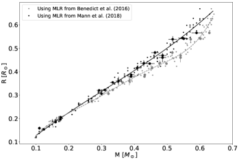
Figure 3: Radius-mass relation for our sample (large dots) and a subset of data from Mann et al. (2015, small dots), selected as described in the text. Black dots are based on mass estimates using the MLR from Mann et al. (2018), whereas grey dots are based on the one from Benedict et al. (2016). The lines show best-fit polynomial, as resulted from the respective MLR. (Details are discussed in Sect. 4)

We also establish a relation between the stellar radius and its effective temperature, see Figure 4. Interestingly, in Figure 4 we identified a discontinuous behaviour between 3200 and 3340 K (gray shaded area), where the radius spans a range from 0.18 to 0.42 $R_{\sun}$  for similar effective temperatures. Considering that our mean measurement error for the radius is $\sim 0.006\,R_{\sun}$, this corresponds to a 40-$\sigma$ difference. We also note that we have done a detailed error analysis of our diameter measurements in Lachaume et al. (2019). We further find that this discontinuity corresponds to a mass of 0.23 $M_{\sun}$, see filled and empty dots in Figure 4.

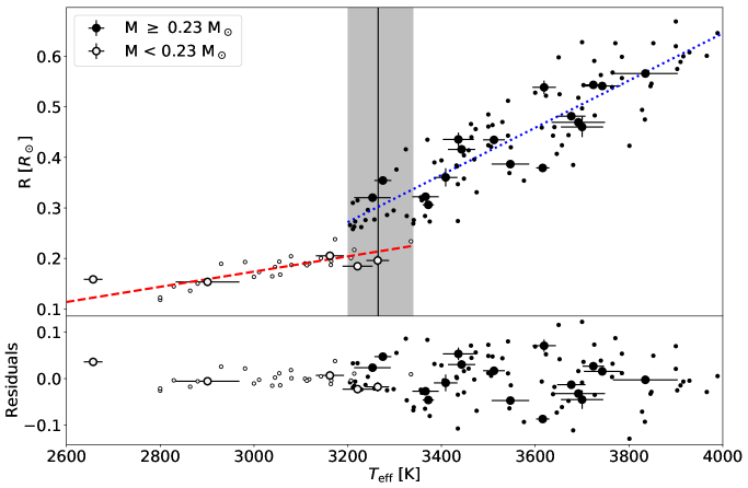
Figure 4: $T_{\rm eff}$ versus radius plot with the stellar mass coded as filled and empty circles, respectively. The lines show fitted polynomials for the two different mass populations (red dashed line for stars with masses $<0.23\,M_{\sun}$ and blue dotted line for stars with masses $\geq 0.23\,M_{\sun}$). Grey shaded area shows the region where we find a possible discontinuity and which we attribute to the transition between partially and fully convective stars. We also added M-dwarfs from Mann et al. (2015) (small dots), see text for details. The lower plot shows the residual after subtracting the polynomials in Eq. 7 from the radius measurements. (Details are discussed in Sect. 4)

To the $T_{\rm eff}$-$R_{\star}$ data we fitted two linear polynomials depending on the mass range, namely for stars with $M_{\star}\geq 0.23\,M_{\sun}$ and $M_{\star}<0.23\,M_{\sun}$. We also tried higher order polynomials, but found in both cases that the higher order coefficients were consistent with zero. We conclude therefore, that for the two cases, the data are best described with two linear polynomials of the form

$$\frac{R_{\star}}{R_{\sun}}=\begin{cases}-1.223(\pm 0.085)+2.700(\pm 0.138)\,\frac{T_{\rm eff}}{T_{\mathrm{eff},\sun}}\\ \qquad\text{for $M_{\star}\geq 0.23\,M_{\sun}$},\\ -0.277(\pm 0.060)+0.869(\pm 0.113)\,\frac{T_{\rm eff}}{T_{\mathrm{eff},\sun}}\\ \qquad\text{for $M_{\star}<0.23\,M_{\sun}$}.\end{cases}$$ (7)

The standard deviation of the residuals are $0.051\,R_{\sun}$ for $M_{\star}\geq 0.23\,M_{\sun}$ and $0.016\,R_{\sun}$ for $M_{\star}<0.23\,M_{\sun}$ and the respective MADs are $0.033\,R_{\sun}$ and $0.0107\,R_{\sun}$. In Figure 5 we show the residuals after subtracting Equation 7 as a function of metallicity. The slope in the data indicates a correlation between metallicity and radius, hence, we calculated the Pearson’s correlation coefficient ($r$). For stars with $M_{\sun}\geq 0.23$ we get $r=0.69$ and for $M_{\sun}<0.23$ $r=0.51$, respectively. We found that stars with higher metallicity have slightly lager radii, and sub-solar metallicity stars lower radii. This correlation is strong for partially convective stars and moderate for fully convective ones. Burrows et al. (2007) proposed that enhanced opacity in atmospheres due to enhanced metallicity could cause inflated radii in giant planets. Given that we find a correlation between metallicity and radius, it is possible to have a similar effect in M-dwarfs. The metallicity effect on the radius can be best described by two linear polynomials of the form:

$$\frac{\Delta R_{\star}}{R_{\star}}=\begin{cases}-0.0060(\pm 0.0093)+0.4166(\pm 0.0462)\,\rm[Fe/H]\\ \qquad\text{ for $M_{\star}\geq 0.23\,M_{\sun}$},\\ 0.0187(\pm 0.0176)+0.2504(\pm 0.0778)\,\rm[Fe/H]\\ \qquad\text{ for $M_{\star}<0.23\,M_{\sun}$}.\end{cases}$$ (8)

In Fig. 6 we show $T_{\rm eff}$-$R_{\star}$, where we corrected the stellar radius for possible metallicity effects using Eq. 8. The best-fit polynomials in this case are:

$$\frac{R_{\star}}{R_{\sun}}=\begin{cases}-1.169(\pm 0.063)+2.620(\pm 0.103)\,\frac{T_{\rm eff}}{T_{\mathrm{eff},\sun}}\\ \qquad\text{for $M_{\star}\geq 0.23\,M_{\sun}$},\\ -0.367(\pm 0.050)+1.041(\pm 0.094)\,\frac{T_{\rm eff}}{T_{\mathrm{eff},\sun}}\\ \qquad\text{for $M_{\star}<0.23\,M_{\sun}$}.\end{cases}$$ (9)

The standard deviation of the residuals are $0.038\,R_{\sun}$ and $0.013\,R_{\sun}$ respectively, which is slightly lower compared to neglecting the influence of metallicity on the radius. The median absolute deviations of the residuals are $0.029\,R_{\sun}$ and $0.008\,R_{\sun}$.

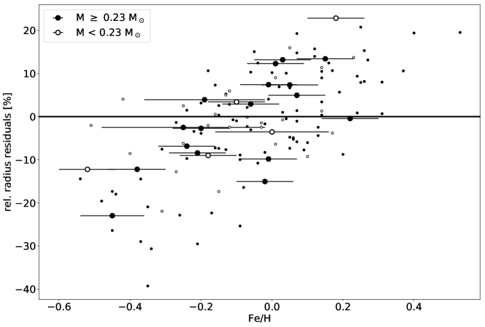
Figure 5: Residuals after subtracting Eq. 7 from the radius measurement as function of stellar metallicity. The Pearson correlation coefficient is $r=0.69$ for $M_{\star}\geq 0.23\,M_{\sun}$ and $r=0.51$ for $M_{\star}<0.23\,M_{\sun}$. Horizontal line represents the case of zero residuals. (Details are discussed in Sect. 4)

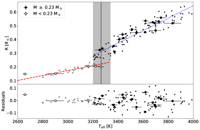
Figure 6: Same as Fig. 4, but correcting the radius for possible metallicity effects. (Details are discussed in Sect. 4)

Based on our observations and our inferred physical parameters, we further show in Figure 7 the empirical HR-diagram for the two different mass populations. We also can identify a transition region in the HR-diagram. We establish the following linear ($\log$ $L_{\star}$)-$T_{\rm eff}$-relation for the two different populations

$$\log L_{\star}=\begin{cases}-6.710(\pm 0.179)+8.318(\pm 0.290)\,\frac{T_{\rm eff}}{T_{\mathrm{eff},\sun}}\\ \qquad\text{for $M_{\star}\geq 0.23\,M_{\sun}$},\\ -6.856(\pm 0.345)+8.099(\pm 0.653)\,\frac{T_{\rm eff}}{T_{\mathrm{eff},\sun}}\\ \qquad\text{for $M_{\star}<0.23\,M_{\sun}$}.\\ \end{cases}$$ (10)

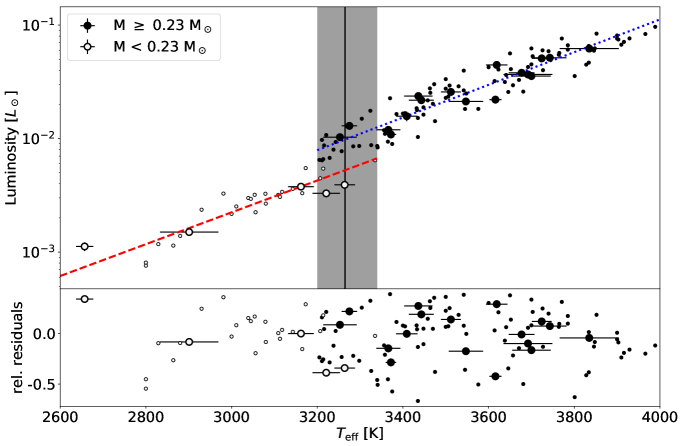
Figure 7: Empirical HR diagram for two different stellar mass populations (filled and empty circles respectively). The red dashed line shows our fitted polynomials for stars with masses $<0.23\,M_{\sun}$ and blue dotted one for masses $\geq 0.23\,M_{\sun}$). We identify a discontinuity (grey shaded area) reflecting the transition region between partially and fully convective stars. Our sample is depicted by the large dots. The sample from Mann et al. (2015) is represented by the smaller dots, which also have their error bars suppressed. Lower plot shows the relative residuals after subtracting Eq. 10 from the luminosity value ($\frac{\rm calc.~{}luminosity-polynomial}{\rm calc.~{}luminosity}$). (Details are discussed in Sect. 4)

4.1 Transition into the fully convective regime

Theoretical stellar evolution predict a transition from partially convective stars into the fully convective stellar regime to occur at stellar mass somewhere between 0.2 $M_{\sun}$ (Dorman et al., 1989) and 0.35 $M_{\sun}$ (Chabrier & Baraffe, 1997), depending on the underlying stellar model. While a partially convective star still resembles a sun-like structure, having a radiative zone and a convective envelope, fully convective stars have no such zone. Our observations indicate that the limit between partially and fully convective regime is around $\approx 0.23\,M_{\sun}$ and between 3200 and 3340 K. The lack of a detection of this transition in previous works can be explained mainly by the fact that very few single M-dwarfs with temperatures below 3270 K have interferometrically measured radii. In fact, Boyajian et al. (2012a) shows only two M-dwarfs with temperatures below this value. Moreover, they include in their work mostly one of the stars (GJ 699) which is in the fully convective regime, as GJ 551 was excluded from most of their analyses. Another reason is that previous radius measurements of fully convective stars relied on eclipsing M-dwarf binaries, where the disentanglement of the respective components is not straightforward. Finally, most radius estimates rely on stellar evolution models rather than direct measurements, i.e. in many cases the radius has not been measured directly.

Furthermore, we find that the linear term of the polynomial in Equation 7 shows a steeper slope for stars with $M_{\star}\geq 0.23\,M_{\sun}$, than for $M_{\star}<0.23\,M_{\sun}$. This is possibly due the fact that stars with $M_{\star}\geq 0.23\,M_{\sun}$ still have a radiative zone which decreases with shrinking $T_{\rm eff}$. For M-dwarfs with $M_{\star}<0.23\,M_{\sun}$ the stars are fully convective, i.e. the convective zone extents towards the core. Therefore, the linear term for M-dwarfs with masses below 0.23 $M_{\sun}$ indicates a more flattened slope. The gentle slope for masses below 0.23 $M_{\sun}$ is consistent with the fact that fully convective stars have similar spectral types due to $\mathrm{H}_{2}$ formation, which also flattens the radius-temperature relation (Chabrier & Baraffe, 2000).

4.2 M-dwarfs in the context of Gaia

In Sect. 3.4 we noticed a considerable difference between $T_{\rm eff}$ for M-dwarfs inferred from Gaia three band photometry (Andrae et al., 2018) and estimates found here and in the literature (Neves et al., 2014; Mann et al., 2015) . Therefore, we establish an empirical calibration relation for stars with very well measured G magnitudes and parallaxes from Gaia. We use these two measurements to calculate the absolute G magnitude $M_{G}$, which we relate to the $T_{\rm eff}$. In Fig. 8 we show $T_{\rm eff}$ as a function of $M_{G}$. The empty circles show the stellar $T_{\rm eff}$ as estimated by Gaia Apsis, whereas the filled circles show our $T_{\rm eff}$ measurements and the ones from Mann et al. (2015). The previously shown discrepancy is also visible in Fig. 8. We determine an empirical relation to obtain $T_{\rm eff}$ from $M_{G}$. In our attempt to find the best relation, we fitted polynomials of different degrees and we calculated their respective AIC and BIC, see Fig. 8. The best relation is described by a cubic polynomial of the form:

$$T_{\rm eff}=10171.7(\pm 1449.6)-1493.4(\pm 410.8)M_{G}\\ +114.1(\pm 38.3)M_{G}^{2}-3.2(\pm 1.2)M_{G}^{3}\\$$ (11)

The standard deviation of the residuals is $53\,T_{\rm eff}$ and the median absolute deviation (MAD) $36\,T_{\rm eff}$. The errors of the polynomial coefficients (closed brackets) are estimated from the covariance matrix.

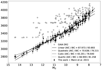
Figure 8: Effective temperature as function of absolute Gaia G magnitude. Empty circles show $T_{\rm eff}$ estimated by Gaia DR2 Apsis. Filled dots show our measurements and the ones from Mann et al. (2015). Lines show polynomial fits of different orders. Their respective AIC and BIC values are given in the legend. (Details are discussed in Sect. 4.2)

Recently, Jao et al. (2018) presented an investigation showing a $\sim$0.05 mag gap in the HR diagram constructed from M-dwarfs using the Gaia DR2. The authors attributed this gap to a possible transition from partially to fully convective low-mass stars. However, recent simulations by MacDonald & Gizis (2018) argued that this gap can be explained by ³He instabilities of low-mass stars rather than the before mentioned transition region. This ³He instabilities are caused by stars with a thin radiative zone, slightly above the transition to fully convective stars. These instabilities can produce energy fluctuations and a dip in the luminosity function (van Saders & Pinsonneault, 2012; MacDonald & Gizis, 2018). In Fig. 9 we show $M_{G}$ over $G_{BP}-G_{RP}$ and mark the region where Jao et al. (2018) found their discontinuity (grey shaded area). The locus of our discovered discontinuity is slightly below the one from Jao et al. (2018). This increases the likelihood of the finding from MacDonald & Gizis (2018) and our claim having observed the transition region between fully and partially convective stars, which should occur slightly below the ³He instability region.

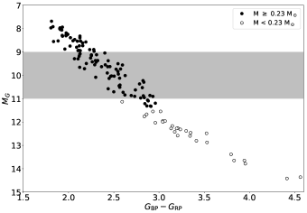
Figure 9: Absolute Gaia G magnitude versus $G_{\rm BP}-G_{\rm RP}$ for M-dwarfs with different masses. Gray shaded area shows the region, where Jao et al. (2018) found a gap in their HR-diagram. (Details are discussed in Sect. 4.2)

5 Conclusion

We have measured physical parameters of 13 M-stars covering the partially and fully convective regime using interferometric measurements from the VLTI and parallaxes from Gaia DR2. Our measurements extend to lower $T_{\rm eff}$ than previous interferometric studies, and we use them augmented with literature data to present improved empirical relations between stellar radius and mass, and between stellar radius and luminosity as a function of $T_{\rm eff}$. Analysing residuals to our relations, we identified a general trend that late-type stars with higher metallicity are slightly inflated, whereas for stars with lower metallicity we measure predominantly smaller radii. We find this correlation to be strong for stars with $M_{\star}\geq 0.23\,M_{\sun}$ and moderate for $M_{\star}<0.23\,M_{\sun}$, respectively. We also found that Gaia $T_{\rm eff}$ values are significantly underestimated ($\approx 8\%$) for M-dwarfs.

The most striking feature we identified in our data is a sharp transition in the relation between $R_{\star}$ and $T_{\rm eff}$, as well as in the empirical HR diagram, which we identify as reflecting the transition between partially and fully convective stars. While previously only a hint for this change had been inferred indirectly, we now have a possible direct observation. We showed that this change happens at $\sim 0.23\,M_{\sun}$ and between 3200 and 3340 K. In this region we measure radii in the range from 0.18 to 0.42 $R_{\sun}$. Thus, our findings put strong constraints on the stellar evolution and interior structure models.

References

- Akaike (1974) Akaike H., 1974, IEEE Transactions on Automatic Control, 19, 716
- Andrae et al. (2018) Andrae R., et al., 2018, A&A, 616, A8
- Benedict et al. (2016) Benedict G. F., et al., 2016, AJ, 152, 141
- Berger et al. (2006) Berger D. H., et al., 2006, ApJ, 644, 475
- Bonfils et al. (2013) Bonfils X., et al., 2013, A&A, 549, A109
- Boyajian et al. (2012a) Boyajian T. S., et al., 2012a, ApJ, 757, 112
- Boyajian et al. (2012b) Boyajian T. S., et al., 2012b, ApJ, 757, 112
- Browning (2008) Browning M. K., 2008, ApJ, 676, 1262
- Buchner et al. (2014) Buchner J., et al., 2014, A&A, 564, A125
- Burrows et al. (2007) Burrows A., Hubeny I., Budaj J., Hubbard W. B., 2007, ApJ, 661, 502
- Chabrier & Baraffe (1997) Chabrier G., Baraffe I., 1997, A&A, 327, 1039
- Chabrier & Baraffe (2000) Chabrier G., Baraffe I., 2000, ARA&A, 38, 337
- Cutri et al. (2003) Cutri R. M., et al., 2003, 2MASS All Sky Catalog of point sources.
- Demory et al. (2009) Demory B.-O., et al., 2009, A&A, 505, 205
- Donati et al. (2008) Donati J.-F., et al., 2008, MNRAS, 390, 545
- Dorman et al. (1989) Dorman B., Nelson L. A., Chau W. Y., 1989, ApJ, 342, 1003
- Dressing & Charbonneau (2013) Dressing C. D., Charbonneau D., 2013, ApJ, 767, 95
- Espinoza & Jordán (2015) Espinoza N., Jordán A., 2015, MNRAS, 450, 1879
- Feroz & Hobson (2008) Feroz F., Hobson M. P., 2008, MNRAS, 384, 449
- Gaia Collaboration et al. (2018) Gaia Collaboration et al., 2018, A&A, 616, A1
- Gallenne et al. (2018) Gallenne A., et al., 2018, A&A, 616, A68
- Hanbury Brown et al. (1974) Hanbury Brown R., Davis J., Lake R. J. W., Thompson R. J., 1974, MNRAS, 167, 475
- Husser et al. (2013) Husser T.-O., Wende-von Berg S., Dreizler S., Homeier D., Reiners A., Barman T., Hauschildt P. H., 2013, A&A, 553, A6
- Irwin et al. (2011) Irwin J., Berta Z. K., Burke C. J., Charbonneau D., Nutzman P., West A. A., Falco E. E., 2011, ApJ, 727, 56
- Jao et al. (2018) Jao W.-C., Henry T. J., Gies D. R., Hambly N. C., 2018, ApJ, 861, L11
- Kesseli et al. (2018) Kesseli A. Y., Muirhead P. S., Mann A. W., Mace G., 2018, AJ, 155, 225
- Koen et al. (2010) Koen C., Kilkenny D., van Wyk F., Marang F., 2010, MNRAS, 403, 1949
- Kopparapu (2013) Kopparapu R. K., 2013, ApJ, 767, L8
- Lachaume et al. (2014) Lachaume R., Rabus M., Jordán A., 2014, in Optical and Infrared Interferometry IV. p. 914631, doi:10.1117/12.2057447
- Lachaume et al. (2019) Lachaume R., Rabus M., Jordán A., Brahm R., Boyajian T., von Braun K., Berger J.-P., 2019, MNRAS,
- Le Bouquin et al. (2011) Le Bouquin J.-B., et al., 2011, A&A, 535, A67
- MacDonald & Gizis (2018) MacDonald J., Gizis J., 2018, MNRAS, 480, 1711
- Mann & von Braun (2015) Mann A. W., von Braun K., 2015, PASP, 127, 102
- Mann et al. (2015) Mann A. W., Feiden G. A., Gaidos E., Boyajian T., von Braun K., 2015, ApJ, 804, 64
- Mann et al. (2018) Mann A. W., et al., 2018, preprint, (arXiv:1811.06938)
- Neves et al. (2014) Neves V., Bonfils X., Santos N. C., Delfosse X., Forveille T., Allard F., Udry S., 2014, A&A, 568, A121
- Newton et al. (2016) Newton E. R., Irwin J., Charbonneau D., Berta-Thompson Z. K., Dittmann J. A., West A. A., 2016, ApJ, 821, 93
- Ricker et al. (2014) Ricker G. R., et al., 2014, in Space Telescopes and Instrumentation 2014: Optical, Infrared, and Millimeter Wave. p. 914320 (arXiv:1406.0151), doi:10.1117/12.2063489
- Schwarz (1978) Schwarz G., 1978, The Annals of Statistics, 6, 461
- Ségransan et al. (2003) Ségransan D., Kervella P., Forveille T., Queloz D., 2003, A&A, 397, L5
- Skilling (2004) Skilling J., 2004, in Fischer R., Preuss R., Toussaint U. V., eds, American Institute of Physics Conference Series Vol. 735, American Institute of Physics Conference Series. pp 395–405, doi:10.1063/1.1835238
- Wright & Drake (2016) Wright N. J., Drake J. J., 2016, Nature, 535, 526
- van Belle & van Belle (2005) van Belle G. T., van Belle G., 2005, PASP, 117, 1263
- van Saders & Pinsonneault (2012) van Saders J. L., Pinsonneault M. H., 2012, ApJ, 751, 98
- von Braun et al. (2011) von Braun K., et al., 2011, ApJ, 729, L26
- von Braun et al. (2012) von Braun K., et al., 2012, ApJ, 753, 171
- von Braun et al. (2014) von Braun K., et al., 2014, MNRAS, 438, 2413