Globular cluster number density profiles using Gaia DR2

Abstract

Using data from Gaia DR2, we study the radial number density profiles of the Galactic globular cluster sample. Proper motions are used for accurate membership selection, especially crucial in the cluster outskirts. Due to the severe crowding in the centres, the Gaia data is supplemented by literature data from HST and surface brightness measurements, where available. This results in 81 clusters with a complete density profile covering the full tidal radius (and beyond) for each cluster. We model the density profiles using a set of single-mass models ranging from King and Wilson models to generalised lowered isothermal limepy models and the recently introduced spes models, which allow for the inclusion of potential escapers. We find that both King and Wilson models are too simple to fully reproduce the density profiles, with King (Wilson) models on average underestimating(overestimating) the radial extent of the clusters. The truncation radii derived from the limepy models are similar to estimates for the Jacobi radii based on the cluster masses and their orbits. We show clear correlations between structural and environmental parameters, as a function of Galactocentric radius and integrated luminosity. Notably, the recovered fraction of potential escapers correlates with cluster pericentre radius, luminosity and cluster concentration. The ratio of half mass over Jacobi radius also correlates with both truncation parameter and PE fraction, showing the effect of Roche lobe filling.

1 Introduction

Globular clusters (GCs) are amongst the oldest known structures in the Universe, believed to have been formed between redshifts of $z\sim 5-10$ (e.g. Kravtsov & Gnedin, 2005). They have long been used as the principal stellar population calibration source against which to compare other systems, or as simple tracer particles to probe the gravitational potential of the systems they inhabit. Through their use, they have contributed to invaluable progress in e.g. early Universe cosmology (Peebles & Dicke, 1968), the formation and evolution of the Milky Way (MW) disc (Freeman & Bland-Hawthorn, 2002) and halo (Searle & Zinn, 1978), and external galaxies (Brodie & Strader, 2006). The present day spatial distribution and motions of GCs provide a dynamical probe of the MW dark matter (DM) potential, the hierarchical assembly of the Milky Way (Moore et al., 2006) and a constraint on the re-ionisation of the Universe (Couchman & Rees, 1986; Spitler et al., 2012).

During the last two decades, the field of GC formation has been reinvigorated due to the discovery that GCs are not simple, spherical, non-rotating stellar systems. An ever increasing number of studies has shown that their stellar populations are anything but simple, with clear evidence for multiple populations due to light element abundance variations and discrete sequences in colour-magnitude space (e.g. Carretta et al., 2009; Gratton, Carretta & Bragaglia, 2012; Bastian & Lardo, 2018). Dynamical studies of GCs have shown the presence of kinematic signatures, concluding that rotation is common in these systems (e.g. Mackey et al., 2013; Fabricius et al., 2014; Ferraro et al., 2018; Kamann et al., 2018; Bianchini et al., 2018). Studies of the dynamical mass-to-light ratios conclude there is no signature of DM in the inner parts of GCs (e.g. Watkins et al., 2015; Kimmig et al., 2015; Baumgardt, 2017), with the discovery of tidal tails around GCs further arguing against significant fractions of DM in at least some GCs (Moore, 1996; Odenkirchen et al., 2001; Shipp et al., 2018).

Nonetheless, the mechanism of GC formation in a DM halo is by no means ruled out, since collisional relaxation pushes the DM to the peripheries where tidal interaction with the MW can effectively strip the entire DM content (Mashchenko & Sills, 2005; Baumgardt & Mieske, 2008). Furthermore, the discovery of extended, spherical stellar halos around some GCs (Carballo-Bello et al., 2012; Kuzma, Da Costa & Mackey, 2018) are in good agreement with models of GC evolution within their own DM halo, in which stars are scattered to large radii and move on long radial orbits as their escape is prevented by their DM halo (Peñarrubia et al., 2017). This has highlighted the need for a comprehensive kinematic study of the outer regions of GCs, which remain largely unexplored.

The spatial structure of GCs has been extensively studied within the Local Group, leading to the discovery of numerous scaling relations (Trager, King & Djorgovski, 1995; Harris, 1996) and the constraining of the GC fundamental plane (Djorgovski & Meylan, 1994; McLaughlin, 2000). Traditionally, the density distribution of GCs has been analysed in the context of isotropic, isothermal sphere models, such as King models (King, 1966). More recent studies found that the outer regions of GCs are more extended than allowed by King models (Elson, Fall & Freeman, 1987; Larsen, 2004) and models with a power law distribution provide a better fit to the outer parts of GCs due to their shallower density fall-off (McLaughlin & van der Marel, 2005; Carballo-Bello et al., 2012; Williams, Barnes & Hjorth, 2012; Kuzma, Da Costa & Mackey, 2018). Once again, studying the outer regions of the GCs is the only way to distinguish between the different models.

King models are isotropic, lowered isothermal models, which are described by a distribution function (DF): $f(E)\propto\exp(-E/s^{2})-1$, for $E<0$ and $f(E)=0$ otherwise. Here $E$ is the specific energy, ‘lowered’ by a truncation energy $\phi_{\rm t}$ (i.e. $E=0.5v^{2}+\phi(r)-\phi_{\rm t}$, where $\phi(r)$ is the specific potential at radius $r$) and $s$ is a velocity scale, which combined with the constant of proportionality in the DF sets the physical scales of the model. This model is fully specified by the dimensionless central potential $W_{0}$, which controls the central concentration (high $W_{0}$ implies more concentrated models). For concentrated models ($W_{0}\gtrsim 5$), $s$ is approximately equal to the central 1-dimensional velocity dispersion. The DF of (isotropic and non-rotating) Wilson models is $f(E)\propto\exp(-E/s^{2})-1+E/s^{2}$, and has a more gradual decline in the density near the tidal radius. Davoust (1977) showed that the King and Wilson models are members of a general family of models in which leading order terms of the exponential are subtracted from the isothemal model. Gomez-Leyton & Velazquez (2014) showed that this can be extended to non-integer terms, leading to a more general class of (isotropic) lowered isothermal model, which has an additional model parameter $g$ (with King and Wilson models recovered for $g=1$ and $g=2$, respectively). Because this additional parameter describes the sharpness of the truncation in energy, it affects mostly the mass and velocity profile at large distances. Gieles & Zocchi (2015) further expanded these models by introducing radial velocity anisotropy as in Eddington (1915) and Michie (1963), multiple mass components as in Da Costa & Freeman (1976) and Gunn & Griffin (1979), and introduced the lowered isothermal model explorer in python (limepy).

The limepy models allow for a more elaborate description of stars near the escape energy, but do not include the effect of the Galactic tidal potential, unlike other models by (e.g. Heggie & Ramamani, 1995; Varri & Bertin, 2009). The tidal field makes the potential in which the stars move anisotropic and it slows down the escape of stars (Fukushige & Heggie, 2000; Baumgardt, 2001), because escape is limited to narrow apertures around the Lagrangian points. As a result, a GC builds up a population of so-called potential escapers (PEs) during its evolution. These are stars that are energetically unbound, but have not yet escaped because their orbits have not come near the Lagrangian points (e.g., Daniel, Heggie & Varri, 2017). These PEs give rise to an elevation of the density and velocity dispersion near the Jacobi radius (Küpper et al., 2010; Claydon, Gieles & Zocchi, 2017). The fraction of PEs in a GC is dependent on the mass of the cluster (approximately) as $M^{1/4}$ (Baumgardt, 2001) and the shape of the Jacobi surface (Claydon, Gieles & Zocchi, 2017), which in turns depends on the Galactic potential and GC orbit (Tanikawa & Fukushige, 2010; Renaud & Gieles, 2015) and for GCs we expect typical fractions of a few per cent (Claydon, Gieles & Zocchi, 2017). The presence of PEs in GCs has been proposed as a way to explain peculiarities in GC outskirts not consistent with the expected behaviour of bound stars even in a generalised lowered isothermal model, such as unusual surface density profiles (e.g. Côté et al., 2002; Küpper, Mieske & Kroupa, 2011), extended structures (Kuzma et al., 2016) and stars with velocities above the escape speed (Meylan, Dubath & Mayor, 1991; Lützgendorf et al., 2012).

In this work, we will make use of data from Gaia DR2 (Gaia Collaboration et al., 2018) to study the outskirts of the sample of Galactic GCs presented in Harris (1996, 2010 version). The use of Gaia proper motions allows us to perform a membership selection which is far more accurate than any other study of GCs on this scale (e.g. Pancino et al., 2017). The density of stars in the outer regions will be combined with existing literature data to obtain a full sampling of GC densities covering the entire system. The resulting density profiles will be modelled using the different types of single-mass models described above to probe for the presence of tidal disturbances and PEs. Importantly, the density profiles will be constructed from a homogeneous dataset, while previous comprehensive works (e.g., Trager, King & Djorgovski, 1995) have been based on a heterogeneous mix of star counts and integrated photometry, and other homogeneous works have been composed of only a few GCs (Carballo-Bello et al., 2012; Miocchi et al., 2013).

This paper is organised as follows: in Section 2 we discuss the use of Gaia data, adopted queries and initial processing. Following this, in Sections 3 and 4 we determine the GC membership selection as well as the construction of density profiles extending from the centre out to $\sim$2 tidal radii. The profiles are then fit using a variety of different single-mass models in Section 5, followed by an analysis of the resulting parameters and their correlations (in Section 6). Finally, Section 7 discusses the results and their implications for the study of initial conditions of GC formation.

2 Data

To study the density profiles of GCs we will make use of data from the Gaia mission (Gaia Collaboration et al., 2016a, b; Lindegren et al., 2018), which contains exquisite data for about 1.6 billion sources covering the full sky. In particular, we make use of the recently released Data Release 2 (DR2) data, which includes spectro-photometry in the $G$, $G_{\rm BP}$ and $G_{\rm RP}$ bands as well as accurate parallaxes and proper motions for stars down to $G=21$ (Riello et al., 2018; Evans et al., 2018; Lindegren et al., 2018). Furthermore, for all bright stars ($G_{\rm RVS}<12$), Gaia measures radial velocities from the Gaia Radial Velocity Spectrometer (RVS) spectrograph (Cropper et al., 2018; Sartoretti et al., 2018). The availability of proper motions on large spatial scales represents a key improvement for the study of GCs, allowing us to study the density in their heavily contaminated outskirts. The use of photometric membership selection followed by spectroscopic confirmation is very inefficient in these regions, leading to low (a few percent) success rates. This impedes a thorough study of GC outskirts, which is where many interesting dynamical processes linked to cluster formation and evolution can be constrained.

We make use of the extensive catalog of GCs from Harris (1996, 2010 version) for our input list of targets. To avoid regions of excessive crowding where Gaia measurements become less reliable, we limit our sample to $|b|>$5 deg, leaving 113 GCs. Each of these targets is queried in the Gaia data archive (https://gea.esac.esa.int/archive/) using a cone search out to a radius of 2.5 times the Jacobi radius ($r_{\rm J}$) determined by Balbinot & Gieles (2018). The dataset is further processed to include tangent plane projection coordinates and extinction values using dust maps from Schlegel, Finkbeiner & Davis (1998) with coefficients from Schlafly & Finkbeiner (2011), on a star by star basis. In heavily extincted regions ($E(B-V)>0.3$) the Schlegel, Finkbeiner & Davis (1998) maps become unreliable, and literature extinction values from Harris (1996, 2010 version) are used instead.

In the determination of cluster-centric coordinates, position angles and ellipticities are assumed to be zero. These parameters are available in the literature, but different studies find different mean values which vary with radius, and often do not probe the cluster outskirts (Harris, 1996; Chen & Chen, 2010). Therefore, we assume each cluster is perfectly spherical, and conduct a detailed study of GC shape in a future work.

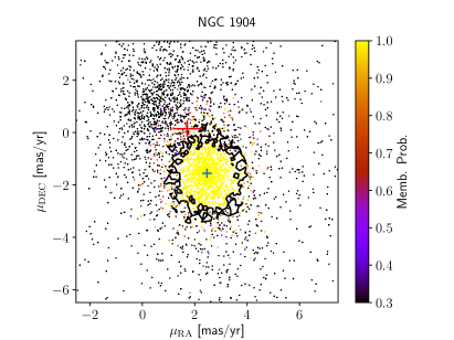
Figure 1: The proper motion distribution of stars in our NGC1904 sample, coloured with the computed membership probability. The sample shown has already been cleaned using CMD isochrone cuts and parallax selections. The blue marker indicates the peak of the GC PM distribution, while the red marker indicates the peak of the background distribution. A contour is drawn for membership probability of 0.9 for reference.

3 Membership selection

A crucial step in the study of GC density profiles is a reliable membership selection. In this work, we first employ a fixed parallax cut to remove nearby stars, followed by a selection in colour-magnitude space and proper motion space. To remove nearby stars we apply a cut to parallax $|\varpi-\varpi_{0}|<2\times\delta\varpi$ with $\varpi_{0}$ the mean parallax of the GC and $\delta\varpi$ the parallax uncertainty. No attempt is made to fit the distribution of parallaxes due to the ongoing characterisation of parallax systematics (Luri et al., 2018).

Colour-magnitude filtering is performed by making use of isochrones with Gaia bandpasses from the Padova library (Marigo et al., 2017), as queried from http://stev.oapd.inaf.it/cmd. For the stellar population parameters of the GCs we make use of metallicities and distances from Harris (2010) and ages taken from (Marín-Franch et al., 2009; VandenBerg et al., 2013). If no age is available, a cluster is assumed to have an age of 13.5 Gyr. For each cluster, we selected member stars in a conservative region around the isochrone with $|(G_{\rm BP}-G_{\rm RP})-(G_{\rm BP}-G_{\rm RP})_{0}|<2\times\delta(G_{\rm BP}-G_{\rm RP})$ at each $G$ magnitude. For this procedure, a minimum colour error of 0.03 is adopted to avoid having an arbitrarily small selection window for bright stars with small photometric errors. We include only stars up to the tip of the Red Giant Branch (RGB) and forego selecting stars on horizontal branch (HB), to avoid including the potentially heavily contaminated regions corresponding to red HBs for metal-rich GCs. A magnitude limit of $G$=20 is adopted to avoid stars with proper motions of poor quality. Furthermore, we do not include a sample cleaning using the phot_bp_rp_excess_factor variable as suggested in Evans et al. (2018). The cleaning of well-behaved single sources will make little difference in halo GCs with good PM separation, but reject a large fraction of sources in crowded regions like the Galactic bulge. Since this is expected to have a large impact on the radial density profiles, we choose to forego selections which are not homogeneous across the cluster field of view.

Following these selections, we use the Gaia proper motions to compute the membership probability of each star. The proper motion cloud is fit using a Gaussian mixture model consisting of one Gaussian for the cluster distribution and another for the Milky Way foreground distribution. Initial guesses for the cluster Gaussian centres are taken from Helmi et al. (2018) where available and using a simple mean within half the Jacobi radius otherwise. Distributions are fit using the emcee python MCMC package, after which membership probabilities for each star in our sample are computed (Foreman-Mackey et al., 2013). The final adopted member samples are selected using a probability cut of 0.5, and made available at https://github.com/tdboer/GC_profiles.

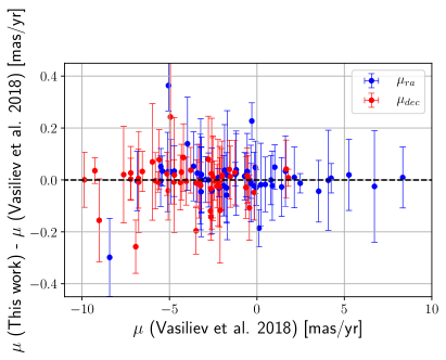
Figure 2: Proper motion comparison between the GCs in common between this work and Vasiliev (2019).

Figure 1 shows the proper motion distribution for an example cluster, NGC1904. The best-fit GC PM peaks are shown as blue and red markers for GC and background sample respectively, while the contours shows the 0.9 member probability. The MCMC fit cleanly separates the cluster and foreground distributions, resulting in a secure sample of member stars with a cut at prob$>$0.5. The GC peak values of ($\mu_{\mathrm{ra}}$,$\mu_{\mathrm{dec}}$) = (2.51$\pm$0.08,-1.51$\pm$0.09) are consistent with values from Helmi et al. (2018).

Figure 2 compares the determined mean proper motions in RA and Dec for GCs in common with the sample from Vasiliev (2019). The errorbars display the uncertainties on the proper motion based on the 16th, 50th, and 84th percentiles from the MCMC runs. There is good agreement between both samples, with overall little scatter in both $\mu_{\mathrm{ra}}$ and $\mu_{\mathrm{dec}}$. Some GCs show large ($>$0.25 mas/yr) uncertainties in our sample, although the peak values are in good agreement with Vasiliev (2019). These are bulge GCs such as NGC6284 and NGC6388 which are low mass, but suffer from excessive ($>$75%) foreground contamination. Given that we determine our PM values using the entire sample within 2.5 times the Jacobi radius, our uncertainties are naturally larger than the values in Vasiliev (2019), where a much smaller spatial area is utilised.

Figure 3 shows the fraction of remaining member stars for each cluster, after successive stages of membership cleaning, as a function of absolute Galactic latitude $|$b$|$. Filled squares show the membership fraction after applying the colour-magnitude filtering using isochrones, relative to the total number of sources within 2.5 times the Jacobi radius. Open circles show the membership fraction after applying the additional proper motion selection described above. The figure shows that the reduction in member stars using a simple CMD cut is roughly a factor of 5 (the mean fraction if 0.18$\pm$0.06), but that the cleaning is least efficient for clusters closest to the MW disk. The filtering using proper motions leads to a further reduction of a factor of two on average (the mean fraction is 0.08$\pm$0.06). However, the reduction is clearly larger for clusters close to the disk (with reductions of a factor $>$5), due to a better separation of cluster and disk stars in proper motion space.

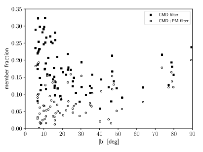
Figure 3: The fraction of member stars in each cluster compared to the total number of stars within 2.5 Jacobi radii, as a function of absolute Galactic latitude $|$b$|$. Member fraction is shown after applying the colour-magnitude isochrone filter, as well as after applying the additional proper motion filter described in Section 3. The mean membership fraction after CMD filtering is 0.18 (a reduction of roughly a factor 5), while the mean membership fraction after CMD+PM filtering is 0.08 constituting a further factor 2 reduction.

4 Number density profiles

With membership probability for our GC sample in place, we construct the radial number density profiles by binning the radial data as a function of distance from the cluster centre. We adopt a fixed number of 50 radial bins, with an equal number of stars in each bin. For ill-sampled or low density GCs, a fixed bin occupation of 10 stars per bin is used instead. We reiterate that sphericity is assumed when computing the radial distance from the cluster centre.

The number density profiles constructed in this way provide a homogeneous coverage of the GC outskirts that is unmatched in other surveys. However, due to the increasing crowding toward the cluster centres, the inner parts of the profiles are incomplete for all but the lowest density clusters (Arenou et al., 2018). To obtain a complete profile for each GC, we complement the Gaia profiles with literature profiles from the Hubble Space Telescope (HST) (Miocchi et al., 2013) and the compilation of ground-based surface brightness profile compilation of Trager, King & Djorgovski (1995). When both are available, Miocchi et al. (2013) profiles are preferred over Trager, King & Djorgovski (1995) profiles since they are more recent. These profiles are stitched to the inner regions of the Gaia profiles to provide a full coverage out and beyond the Jacobi radius. To stitch the profiles, we first need to determine out to which radius the Gaia data is reliable and complete. We make use of the comparison between Gaia and HST data for 26 clusters performed in Arenou et al. (2018), which shows that densities of 10⁵ stars/deg² are roughly 80% complete at $G=20$ mag. Therefore, we assume the Gaia is free from radius dependent completeness effects outside this radius and adopt this density threshold as the cutoff for the Gaia profiles. Figure 4 displays a zoom of the spatial distribution of our NGC1904 sample after membership selection, clearly showing the incompleteness of the data in the central regions due to crowding. Using the density criterium from Arenou et al. (2018), we compute an innermost usable radius of 2.9^′ for this cluster, which is shown in the figure as a red circle. Given that the completeness depends on more than just a simple function of local stellar density (e.g. scanning law coverage, extinction, foreground contamination), we adopt a default inner radius of 2 arcmin for GCs of low density, inside of which we will not use the Gaia data. The adopted innermost usable radii are presented in Table LABEL:GCpars for each GC.

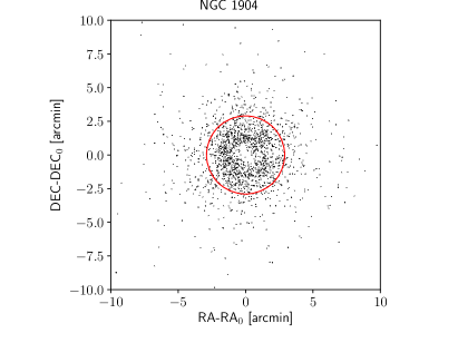
Figure 4: Zoom of the inner regions of the spatial coverage of our NGC 1904 sample, after membership selection. A hole due to incompleteness is clearly visible in the cluster centre. The red circle indicates the innermost usable Gaia radius of 2.9^′, computed following the density prescription from Arenou et al. (2018).

Following this, the Gaia profiles are then tied together with literature profiles by using the overlapping region of both datasets (outside the inner usable Gaia radius) to calibrate the heterogeneous literature data to the homogeneous Gaia system. Within the overlap region, the literature profile data is interpolated to the same radial values as the Gaia profile, allowing us to compute a scaling fraction for each radial bin. The adopted scaling fraction is taken to be the average of all the individual fractions, after which the entire literature profile is scaled. Following this, the two profiles are combined, taking the scaled literature values within the innermost usable radius and the Gaia profile outside, taking care to rescale the number densities in overlapping bins straddling the adopted radius. Figure 5 shows the density profile of NGC1904 as determined from Gaia data (in blue triangles), along with the existing literature profile from Miocchi et al. (2013) as red squares. The Gaia profile clearly becomes incomplete in the inner regions, as evidenced by the drop in density at a radius of $\sim 1^{\prime}$. The green circles show the combined density profile adopted for the cluster, to which mass models will be fit. From Figure 5 it is clear that using the Gaia membership allows us to make use of reliable stellar density data almost 1.5 order of magnitude below the background of the HST data, showing the added value of proper motion information.

In tying the two profiles together, we are making the implicit assumption that both profiles follow the same underlying number density distribution. While not necessarily true, we believe this to be a reasonable assumption, given that the Gaia profile is calculated from bright stars and the attached luminosity profiles are also dominated by bright stars. Furthermore, the effects of mass segregation should not be significant as the stars in both datasets have a small range of stellar mass. For these reasons, we believe the difference between the two profiles are small and our approach is justified.

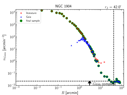
Figure 5: The number density profile of NGC1904. Blue triangles show the profile as obtained from Gaia DR2 after the selections for parallax, proper motion and colours described in section 3. Red squares show the HST number density profile from (Miocchi et al., 2013), scaled to the Gaia profile using all points in the overlapping region outside the Gaia inner usable radius (shown in Figure 4, and indicated by the solid black arrow). Finally, the green circles shows the combination of both profiles, which will be used to fit mass models. For reference, the vertical dashed line shows the Jacobi radius from Balbinot & Gieles (2018) while the dashed horizontal line shows the background level estimated using stars between 1.5 and 2 Jacobi radii.

5 Dynamical model fits

We will consider different types of single-mass models to fit the number density profiles of our GC sample. First off, we consider the King and the isotropic and non-rotating Wilson models, which are often used to fit the spatial distributions of both GCs and dwarf galaxies (King, 1966; Wilson, 1975). King and Wilson models provide a fairly simple description of GC morphology, with their shape entirely determined by the dimensionless central potential $W_{0}$ (high $W_{0}$ implies more concentrated models). For some GCs, Wilson models have been shown to fit the outer parts of GCs better than King models, due to their shallower density fall-off (McLaughlin & van der Marel, 2005). King models have been fitted to Galactic GCs by numerous previous works (e.g. Djorgovski, 1993), while Wilson models have been fitted to the entire Trager, King & Djorgovski (1995) data set by McLaughlin & van der Marel (2005). However, given the updated profiles for the GCs presented here, we have refit for the parameters of the King and Wilson models. We will also fit the isotropic, single-mass limepy models to the data and simultaneously fit on $W_{0}$ and the truncation parameter $g$.

The second class of models we fit to the data are models with the inclusion of Potential Escapers (PEs), as recently presented in Claydon et al. (2019). These models allow for a more elaborate description of stars near the escape energy including the effect of marginally unbound stars. These spherical potential escapers stitched models (hereafter spes models) have an energy truncation similar to the models discussed above, with the fundamental difference that the density of stars at the truncation energy can be non-zero. More importantly, the models include stars above the escape energy, with an isothermal DF that continuously and smoothly connects to the bound stars. Apart from $W_{0}$, the model has two additional parameters $B$ and $\eta$. The value of $B$ can be $0\leq B\leq 1$, where for $B=1$ there are no PEs (i.e. the DF is the same as the King model) and for $0\leq B<1$, the model contains PEs. The parameter $\eta$ is the ratio of the velocity dispersion of the PEs over the velocity scale $s$ (see above) and it can have values $0\leq\eta\leq 1$. For $\eta=0$ there are no PEs, and (for fixed $B$) the fraction of PEs correlates with $\eta$. For a fixed $\eta$, the fraction of PEs anticorrelates with $B$ for $B$ close to 1. For smaller $B$, the fraction of PEs is approximately constant or correlates slightly with $B$ (for constant $\eta$). Finally, in the presence of PEs the spes models are not continuous at $r_{\rm t}$, but the models have the ability to be solved (continuously and smoothly) beyond $r_{\rm t}$ to mimic the effect of escaping stars (see Claydon et al., 2019, for details). We solve the models out to 25 times the Jacobi radii determined by Balbinot & Gieles (2018) to take into account the projected density in front of the cluster and allow a smooth transition between cluster and background counts.

The models are fit to the combined number density profiles using the emcee python MCMC package (Foreman-Mackey et al., 2013), fitting for the model parameters (one for the King/Wilson models, two for limepy and three for spes models), the radial scale (we use the tidal radius as a fitting parameter) and the vertical scaling of the profile. A constant contamination level is defined by taking the average stellar density between 1.5 and 2 Jacobi radii, where we expect the GC contribution to be negligible. Computed background levels are presented in Table LABEL:GCpars. In the case of the spes models, we also directly fit for the cluster tidal radius, without making any a priori assumption about the Jacobi radius.

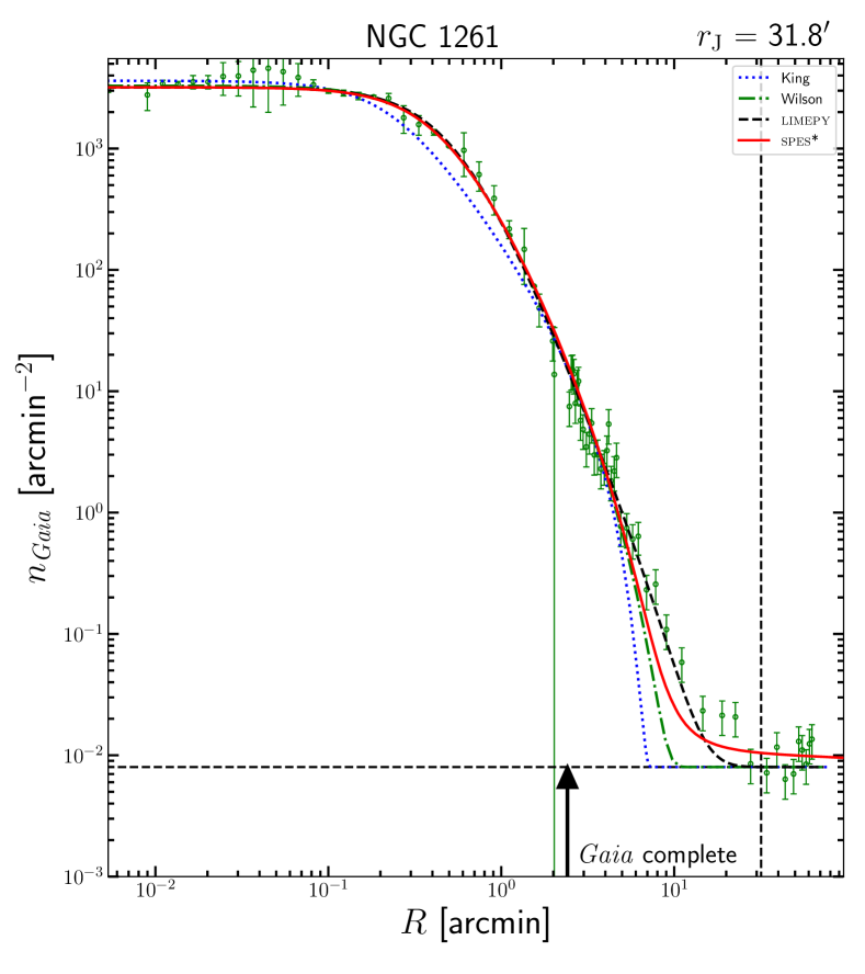
Figure 6: The number density profile of NGC 1261 with best-fit dynamical models. Blue and green dashed lines indicate King and Wilson models respectively, with parameters taken from McLaughlin & van der Marel (2005). The solid black line shows the best-fit limepy model, while the red solid line shows the spes model fit. The model indicated by an * is the one with the lowest reduced $\chi^{2}$ value. In this case, the best-fit Limepy model has a $W_{0}$ of $3.63\pm 0.41$ while the Wilson model has $W_{0}$=5.09$\pm$0.03). The best-fit spes model has $W_{0}=4.99\pm 0.10$, $\eta=0.23\pm 0.01$ and $\log_{10}(1-B)=-2.59\pm 0.23$. This results in a PE fraction of 0.25$\pm$0.09 per cent of the total mass. Finally, the derived tidal radius is $r_{\rm t}=51.51\pm 4.52^{\prime}$, which is slightly larger than the estimated Jacobi radius of $r_{\rm J}=31.80^{\prime}$ from Balbinot & Gieles (2018).

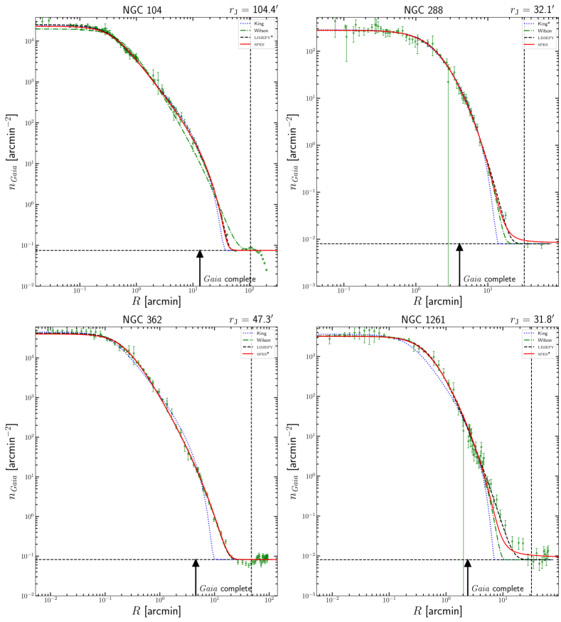
Figure 18: The number density profiles of all GCs with converged fit parameters, along with best-fit dynamical models overlaid. The errorbars on individual data points are Poisson uncertainties for each radial bin. The blue and green dashed lines indicate King and Wilson models respectively, while the solid black line shows the best-fit limepy model and the red solid line shows the spes model fit. The model indicated by an * is the one with the lowest reduced $\chi^{2}$ value. The parameters used for the models are given in Table LABEL:GCpars, along with the derived innermost reliable radius and tidal radius.

Figure 6 shows an example number density profile fit for NGC 1261 with best fitting models overlaid. The errorbars on individual data points are Poisson uncertainties for each radial bin. King and Wilson models with parameters taken from McLaughlin & van der Marel (2005) are shown as blue and green dashed lines respectively, while the limepy model is shown as the solid black line. The red line shows the best-fit spes model including PEs. It is clear from Figure 6 that King and Wilson models do not manage to fit the outermost density profile, truncating at radii of $\approx$5 and 9^′ respectively, which falls far short of the 31.8^′ Jacobi radius from Balbinot & Gieles (2018). Even the limepy model does not manage to reproduce the outer slope of the number density profile completely. However, the spes model does provide a good fit of the GC profile, both in the very centre and in the outskirts. The best-fit parameters of the spes model are $W_{0}=4.99\pm$0.10, $\eta=0.23\pm$0.01 and $\log_{10}(1-B)=-2.59\pm 0.23$, resulting in a fraction of PEs of $0.25\pm 0.09\%$ of the total mass. The derived tidal radius of the model is $r_{\rm t}=51.51\pm 4.52^{\prime}$, indicating this cluster is much more extended (factor of 5-10 larger $r_{\rm t}$) than can be inferred from simple single-mass models like King and Wilson. The number density profiles and model fits are shown for all GCs in Figure 18 in Appendix A.

6 results

Our analysis of all GCs in the Harris catalogue with $|b|>5$ deg (113 clusters) resulted in PMs and number density profiles for 81 clusters. The remaining GCs are rejected from our final sample due to a variety of reasons, including being too distant to contain enough stars in Gaia DR2, suffering from poor scanning law coverage or sampling incompleteness resulting in profiles that could not be tied to literature values. The remaining GCs have been fit using single-mass models, with model fits shown in Figure 18. The best-fit parameters of the models are given in Table LABEL:GCpars in Appendix B.

Analysis of the fits in Figure 18 shows that King and Wilson models are typically not a good fit to our GC density profiles, especially in the outskirts. In almost all cases, a limepy or spes model results in a better or equally good fit. Nonetheless, there are some GCs for which a King or Wilson model results in the lowest $\chi^{2}$ value (indicated by the * in the plot legend). In those cases, the profiles of all fitted models are very similar, but the simpler model is preferred due to the lower number of model parameters. Figure 7 shows the reduced $\chi^{2}$ values for the different model fits as a function of the reduced $\chi^{2}$ value computed from the comparison between the Wilson model with McLaughlin & van der Marel (2005) parameters and our profile. The King models provide worse fits for the majority of GCs (as found already by McLaughlin & van der Marel, 2005), although a subsample of our clusters are fit much better by King than Wilson models. The fits for limepy and spes models result in fits better than Wilson profiles for all but 2 GCs. Furthermore, for the majority of GCs, a spes model shows a smaller reduced $\chi^{2}$ value than a limepy model, indicating the outer GC structure is better matched with the inclusion of PEs. Therefore, we can conclude that both King and Wilson models are too simplistic, and limepy or spes models are needed to explain the distribution of GC stars simultaneously in the inner and outer regions.

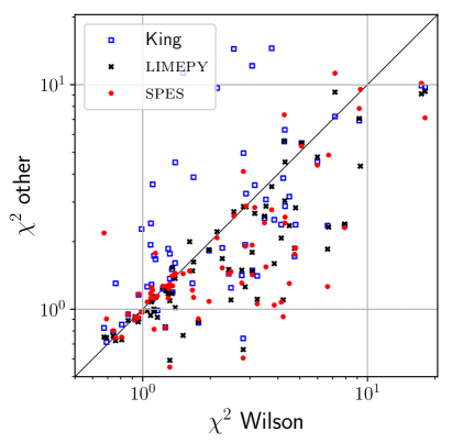
Figure 7: Comparison between the reduced $\chi^{2}$ values of the Wilson fits and those for the other model fits. Points below the line indicate a fit better than Wilson, while points above indicate a fit worse than Wilson. For the majority of GCs, spes models result in a better $\chi^{2}$ than limepy models.

6.1 Model comparisons

We can compare the structural parameters of the different model fits, and correlate them with literature values. First off, Figure 8 shows the comparison between the $W_{0}$ parameter as presented in Table LABEL:GCpars as derived from the fits to our new profiles and the literature values from McLaughlin & van der Marel (2005). The recovered values are in good agreement to the literature values for most of the GCs, with a few notable outliers at low $W_{0}$ such as NGC 6101 and NGC 6496 which were notably incompletely sampled in McLaughlin & van der Marel (2005).

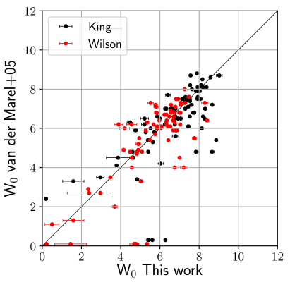
Figure 8: Comparison between the $W_{0}$ parameter for King and Wilson as derived from our fits and the values from McLaughlin & van der Marel (2005). The solid line indicates the one to one correlation.

Next, Figure 9 shows the values of the 3D half mass radius for each of the different model fits, in comparison to effective half mass radii from Harris (1996, 2010 version) (which are mostly from McLaughlin & van der Marel (2005)), multiplied by a factor of 4/3 to correct for the radius projection. We note that we are neglecting any possible effect due to mass segregation. Our models all fall along the one-to-one correlation line, indicating good agreement between the literature and our models.

Given the large radial extent of the Gaia DR2 data, it is insightful to look at the tidal radii as derived from our fits. In Figure 10 we show the tidal radius of each model in comparison to the values of the Jacobi radius as determined by Balbinot & Gieles (2018). For reference, the Jacobi radii are computed following R_J = [G M_cluster / 2* 220²]^1/3 R${}_{GC}^{2/3}$, in which M_cluster is the present day mass of the GC and R_GC is the Galactocentric radius. The top panel of Figure 10 indicates the truncation radii of King fits is too small, owing to the intrinsic shape of the model. Values derived from Wilson fits are more diverse, with roughly half showing larger truncation radii than Jacobi radii. Comparison of model fits in Figure 18 makes it clear that McLaughlin & van der Marel (2005) parameters are simply not a good representation of the outskirts of many of these GCs, such as NGC6121.

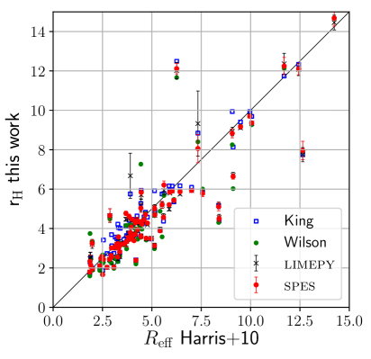
Figure 9: Comparison between half mass radius R_half as derived from our fits and the values from Harris (1996, 2010 version). The solid line indicates the one to one correlation.

The bottom panel of Figure 10 shows that tidal radii from limepy fits are mostly in agreement with the Jacobi radii estimates from Balbinot & Gieles (2018). The spes fits result in tidal radii which are mostly below the Jacobi radii but with a clear subset with values above or in agreement with the estimates based on the mass and orbit. The difference between the two groups is related to fraction of PEs ($f_{\rm PE}$) recovered in the best-fit. As expected, a larger $f_{\rm PE}$ leads to a decrease in the fitted tidal radius. This can be understood by considering that the PEs can have an energy greater than the binding energy and can therefore reside at distances greater than the tidal radius. Conversely, for limepy fits, the tidal radius will be larger to model the PEs as if they were bound stars. Fitting the density of these stars as bound objects therefore leads to an overestimate of the tidal radius when using limepy models. Models with $\log_{10}(f_{\rm PE})>-3$ (i.e. more than 0.1 per cent) are shown as full red symbols, and consistently show tidal radii smaller than Jacobi radii.

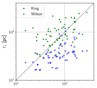
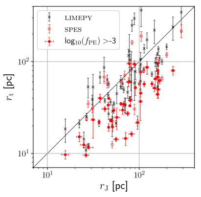
Figure 10: Comparison between $r_{\rm t}$ as derived from our fits and the R_J values from Balbinot & Gieles (2018). GCs with large ($>$0.1 percent) fractions of PEs are shown as solid red symbols. We note that King and Wilson models are not fits, but simply use parameters as given in McLaughlin & van der Marel (2005).

6.2 Structural parameters

We will now focus on the results from the limepy and spes fits, and analyse them further to look for trends of GC structural parameters as a function of environment or initial parameters.

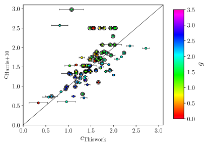
Figure 11: Comparison between the concentration parameter $c$ as defined by log₁₀($r_{\rm t}$/$r_{\mathrm{core}}$) for our spes models and those from Harris (1996, 2010 version). Higher values of $c$ indicate a higher concentration, with $c=2.5$ typically classified as core collapse GCs. Colours indicate the truncation parameter $g$ from limepy fits. GCs with large ($>$0.1 percent) fractions of PEs are shown as points with an additional circle around them.

First off, in Fig. 11 we compare the recovered concentration $c$ of our spes models to those derived by Harris (1996, 2010 version). Concentration $c$ is defined as log₁₀($r_{\rm t}$/$r_{\mathrm{core}}$) with $r_{\mathrm{core}}$ being the core radius (the distance from the cluster centre at which the surface brightness drops by a factor of two from the central value). In the definition of $c$ employed in McLaughlin & van der Marel (2005) the King core radius is used, but the difference between the two quantities is negligible for all but the lowest $W_{0}$ GCs. There is good agreement between the two concentration parameters, indicating the concentration is largely consistent in between King and spes models. Nonetheless, there is noticeable scatter around the 1:1 line due to the different tidal radii used, which are in some cases off by a factor of 2 or more. The colours of points in Fig. 11 represents the limepy truncation parameter $g$, which is a measure of the extent of the cluster halo. The figure shows that more concentrated GCs typically show a lower value of $g$ (i.e. are for instance more King-like than Wilson-like), but there is clear variation in $c$ between GCs with the same truncation parameter $g$. This indicates that $g$ alone does not provide a unique measure of cluster concentration, but does anti-correlate with increased concentration.

Next, we discuss the parameters derived for the limepy and spes model fits, as shown in Figure 12 in both scatter plots and histograms. The truncation parameter $g$ correlates with the tidal radius, as expected, while $W_{0}$ weakly correlates with both half-mass and tidal radius. The best-fit limepy fit parameters result in half mass radii which peak at $\approx$5 pc and tidal radii covering a range in between 30$-$130 pc. The GC sample from Harris (1996, 2010 version) covers a variety of morphologies, with a wide range in both dimensionless potential $W_{0}$ and $g$. Strikingly, there is a clear correlation between the two parameters, with GCs with high $W_{0}$ having lower truncation parameter $g$ on average. The single GC showing both low $W_{0}$ and $g$ is Pal 11, for which the available data is low quality due to its distance and location close to the Galactic bulge.

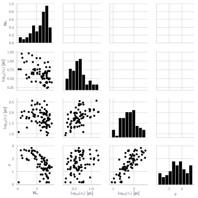
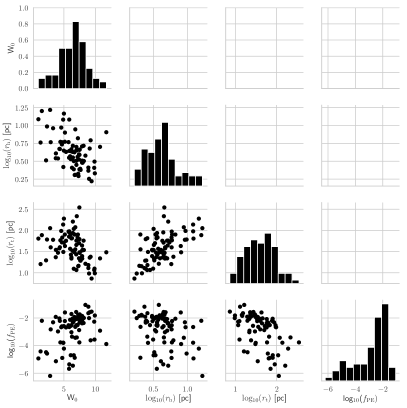
Figure 12: Scatter matrix plots of limepy and spes fit parameters.

The spes fit parameters are shown in the bottom panels of Figure 12. Once again, half mass radii peak around values of 5 pc, while tidal radii peak at values around 30-50 pc, consistent with results from Figures 9 and 10. The fraction of PEs in the spes fits shows a peak at $\log_{10}(f_{\rm PE})=-2$ with a long tail towards negligible PE fractions. The fraction of PEs does not strongly correlate with $W_{0}$ like the $g$ parameter of the limepy fits, although higher values of $f_{\rm PE}$ tend to be found for GCs with a higher value of $W_{0}$.

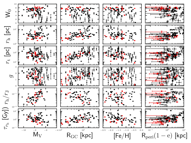
Figure 13: Correlation plots showing structural values from the limepy fits ($W_{0}$, half mass radius $r_{\mathrm{h}}$, tidal radius, $g$, fractional $r_{\mathrm{h}}$ and half mass relaxation time $\tau_{\mathrm{r_{h}}}$) versus global values (integrated $V$-band luminosity, Galactocentric radius, metallicity and pericentre distance). The red points show core-collapse clusters, according to Harris (1996, 2010 version).

Besides structural parameters, we can also compare the best-fit model values to environmental and global parameters. To that end, we have compiled a list of parameters from Harris (1996, 2010 version) including integrated $V$-band luminosity, Galactocentric radius and metallicity. Furthermore, we also consider orbital information from Vasiliev (2019) and compute GC pericentre radii. Figure 13 displays the limepy parameters as a function of the environmental parameters, while Figure 14 displays the spes parameters. Besides basic structural parameters, we also included the half mass relaxation time, following the prescription by McLaughlin & van der Marel (2005) who in turn followed Binney & Tremaine (1987) ($\tau_{\mathrm{r_{h}}}/{\rm yr}$ = $\left[2.06\times 10^{6}/\ln(0.4M_{\rm tot}/m_{\star})\right]m_{\star}^{-1}M_{\rm tot}^{1/2}\mathrm{r_{h}}^{3/2}$ with m_⋆ = 0.5M_⊙).

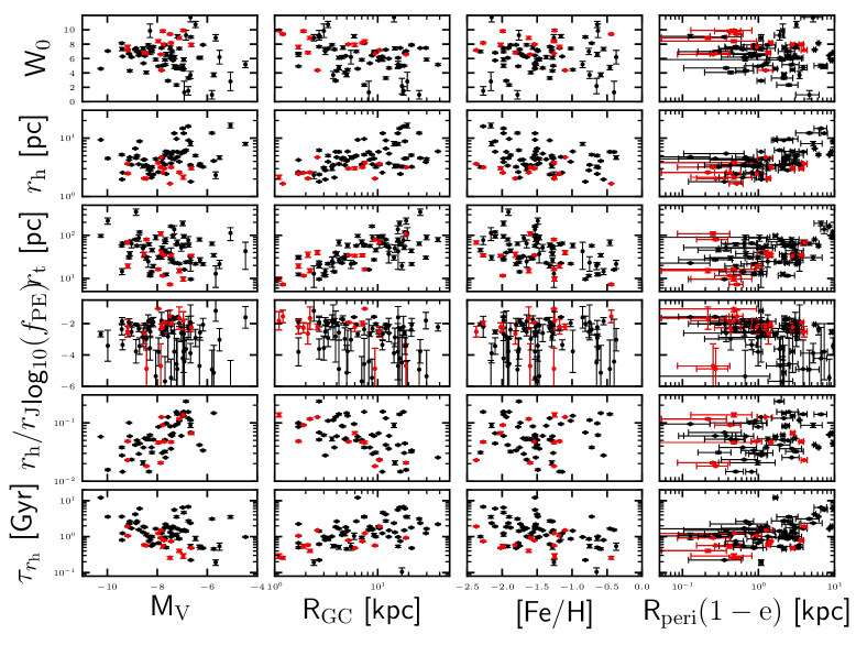
Figure 14: Correlation plots showing structural values from the spes fits ($W_{0}$, half mass radius $r_{\mathrm{h}}$, tidal radius, f_PE, fractional $r_{\mathrm{h}}$ and half mass relaxation time $\tau_{\mathrm{r_{h}}}$) versus global values (integrated $V$-band luminosity, Galactocentric radius, metallicity and pericentre distance). Black points show all GCs, while red points show core-collapse clusters.

It is clear once again that the sample of 81 GCs displays a wide variety of morphologies and covers a range in both luminosity, metallicity and Galactocentric radius. There are a number of clear correlations in Figure 13, some of which are obvious. For instance, $r_{\rm t}$ correlates with R_GC given the weaker tidal field at large Galactocentric radius(von Hoerner, 1957). Additionally, we also see that metallicity correlates with half mass and tidal radii, which is likely a manifestation of the underlying correlation between Galactocentric radius and metallicity (van den Bergh, 2011). GCs with brighter integrated $V$-band luminosity typically display higher values of truncation parameter $g$ and lower values of $r_{\mathrm{h}}$/$r_{\mathrm{J}}$, due to their smaller half-mass radii leading to bright cores.

There are several other correlating parameters among the best-fit limepy parameters. The dimensionless potential $W_{0}$ correlates weakly with $V$-band luminosity, and GC pericentre radius. The concentration sensitive limepy $g$ parameter clearly correlates with Galactocentric radius $R_{\mathrm{GC}}$ showing that outer MW GCs are less concentrated than those more inward, similar to results from Djorgovski & Meylan (1994); van den Bergh (2011). The $r_{\mathrm{h}}$/$r_{\mathrm{J}}$ parameter also correlates with R_GC, with lower values found at larger Galactocentric radius. Similar to Baumgardt et al. (2010) we see a group of GCs with both a large Galactocentric radius and high $r_{\mathrm{h}}$/$r_{\mathrm{J}}$. The GCs found in this branch preferentially display lower $W_{0}$ and $g$ than the bulk of the clusters. Unfortunately, our sample does not include as many GCs in this group as in Baumgardt et al. (2010) due to their large distance pushing them out of the observable window of Gaia. Finally, the limepy truncation parameter $g$ also correlates with Galactocentric radius, with more King-like GCs found preferentially at smaller radii.

Figure 14 shows that some of the same correlations are present in the best-fit spes parameters. The correlations with tidal radius are more pronounced in the spes fits, given the results of Figure 10. The fraction of PEs correlates weakly with the $V$-band luminosity in the sense that higher luminosity GCs have less PEs. The fraction $f_{\mathrm{PE}}$ also correlates with both the Galactocentric radius and pericentre distance, with larger distance leading to a lower fraction of PEs, likely due to experiencing weaker gravitational fields. The pericentre distance also correlates with half-mass radius $r_{\mathrm{h}}$ and W₀, showing a higher W₀ and smaller $r_{\mathrm{h}}$ for GCs with small pericentres. Therefore, the Galactic tidal field exerts an influence not just on the very outskirts of GCs but also further into the cluster centre.

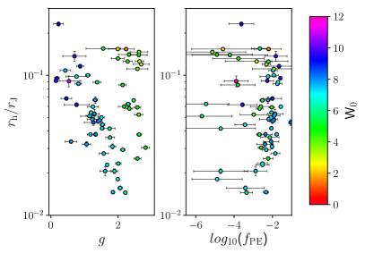
Figure 15: Comparison between the ratio $r_{\mathrm{h}}$/$r_{\mathrm{J}}$ and $g$ or $f_{\mathrm{PE}}$ for the limepy and spes models respectively. The colour of individual points indicates the value of $W_{0}$.

To investigate the parameters in more detail, Figure 15 shows $r_{\mathrm{h}}$/$r_{\mathrm{J}}$ as a function of the limepy truncation parameter $g$ and the spes fraction of PEs. In the figure, points are coloured according to the dimensionless potential $W_{0}$ for each model fit. The left panel shows that truncation parameter and $r_{\mathrm{h}}$/$r_{\mathrm{J}}$ are clearly correlated for GCs with similar $W_{0}$, with for instance a diagonal sequence for systems with $W_{0}=7-8$. There is also a correlation with $W_{0}$ at fixed truncation parameter. The right panel of Figure 15 shows the correlation between $r_{\mathrm{h}}$/$r_{\mathrm{J}}$ and the fraction of PEs. Looking just at GCs with a fraction of PEs higher than 0.1% we see a weak correlation with $r_{\mathrm{h}}$/$r_{\mathrm{J}}$. GCs with higher $r_{\mathrm{h}}$/$r_{\mathrm{J}}$ are more likely to be Roche filling, in which case a higher fraction of PEs is expected, and inferred.

Furthermore, Figure 16 shows the limepy truncation parameter $g$ as a function of the cluster remaining mass fraction of Balbinot & Gieles (2018), which is an indication of how evolved the cluster is. Simulations by Zocchi et al. (2016) indicate that the cluster truncation changes over time, with $g$ being smaller for more evolved clusters. Clusters start of with high $g$, which decreases to King-like values as they fill their Roche volume. This is indeed what we see in Figure 16, with more unevolved clusters showing Wilson-like profiles and evolved cluster with $\mu<$0.3 displaying King-like $g$. The 3 GCs with high g at low $\mu$ are pal$\_$1, NGC 6366 and ic 1276, which suffer from high background contamination or poor sampling in Gaia, which may affect the recovered $g$. A more thorough study of these GCs with Gaia DR3 would be beneficial to obtain a more accurate inner profile shape.

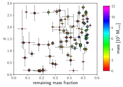
Figure 16: Comparison between the remaining mass fraction $\mu$ from Balbinot & Gieles (2018) and the limepy truncation parameter $g$. Lower values of $\mu$ indicate a larger fraction of the cluster has been lost, consistent with a more evolved cluster. Colours indicate the cluster mass from Harris (1996, 2010 version). GCs with large ($>$0.1 percent) fractions of PEs are shown as points with an additional circle around them.

Figure 17 shows a comparison between the integrated cluster mass from Harris (1996, 2010 version) and the ratio $r_{\mathrm{h}}$/$r_{\mathrm{J}}$ from the limepy models. A clear correlation is visible, with only little dependence on $f_{\mathrm{PE}}$, indicating that the $r_{\mathrm{h}}$/$r_{\mathrm{J}}$ fraction is driven primarily by mass. We see that cluster with lower mass are more Roche filling than the high mass clusters, or alternatively that massive clusters are under-filling their tidal radius. This could be linked to the effects of 2-body relaxation, with which larger masses have a longer relaxation time, which leads to a lower Roche lobe filling.

7 Conclusions and discussion

In this work, we have utilised data from Gaia DR2 to study the number density profile of GCs from the sample of Harris (1996, 2010 version). The proper motion selected samples of GC members are combined with literature data from Trager, King & Djorgovski (1995) and Miocchi et al. (2013) to obtain a full sampling of the density profile (see Section 4). This is the first time that GC profiles are investigated using data covering both the inner regions and outskirts simultaneously.

We have fit the combined density profiles using a variety of single-mass models, including often-used King and Wilson models, as well as the recently introduced limepy models. Finally, we also utilise the recently developed spes models (see Section 5), which include a prescription for the presence of PE stars, essential for reproducing the outskirts of GCs.

The individual cluster fits in Appendix A show that the King and Wilson model fits of McLaughlin & van der Marel (2005) are not sufficient to explain the density profile in the outskirts of GCs. The limepy and spes models fare better at reproducing the full density profile of our sample of GCs, with the spes models in particular providing a better fit to low mass clusters like NGC 1261 (see also Figure 7). It is clear that including PEs in mass models is crucial for fully modelling GCs with a high Roche filling factor (see also Hénault-Brunet et al., 2019). In section 6 we have compared the structural parameters of the different model fits to look for correlations with environmental parameters. Comparison of recovered tidal radii (Fig. 10) makes it clear the fraction of PEs has a strong influence on the GC tidal radius, with fractions of 0.1 percent (by mass) leading to significantly smaller tidal radii. Comparison of best-fit parameters with environmental parameters also reveals correlations between some parameters, some of which are known and some of which are new (see Section 6.2).

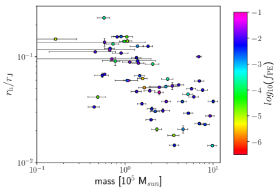
Figure 17: Comparison between the mass of the clusters from Harris (1996, 2010 version) and the ratio $r_{\mathrm{h}}$/$r_{\mathrm{J}}$ from the limepy models. The colour of individual points indicates the value of $f_{\mathrm{PE}}$ from spes models.

For instance, the comparison between limepy dimensionless potential $W_{0}$ and truncation parameter $g$ in Figure 12 shows that the expected correlation is not linear but levels out on both ends. Furthermore, it is clear that the sample of GCs cannot be described well by models using a single truncation parameter, such as King ($g=1$) or Wilson ($g=2$) models. The truncation parameter itself depends on both integrated $V$-band luminosity (probing the GC mass) and position within the Galaxy.

Figure 14 shows that the fraction of PEs in a GC depends on both environment (pericentre distance) and structure (integrated brightness). As expected, closer pericentres result in stronger tidal fields and therefore a higher PE fraction. Finally, Figure 15 shows us that high PE fractions are found in GCs with high $r_{\mathrm{h}}$/$r_{\mathrm{J}}$, but that this is also dependant on $W_{0}$.

The analysis of structural and environmental parameters shows clear effects of current location and experienced tidal field on the properties of the cluster outskirts, such as tidal radius and fraction of PEs. The correlation between truncation parameter $g$ and Galactocentric radius shows that more King-like GCs are found preferentially at smaller radii, while more Wilson-like GCs are found further out. Figures 13 and 14 also show that more distant GCs are typically less concentrated than those more inward, similar to results from van den Bergh (2011). Similarly, the fraction of PEs correlates with environment, with larger distance leading to a lower fraction of PEs. This can be understood by taking into account the weaker Galactic tidal field at large distance.

Strikingly, the pericentre distance correlates with both half-mass radius and $W_{0}$, with low pericentre distance leading to a higher $W_{0}$ and smaller $r_{\mathrm{h}}$. This indicates that the Galactic tidal field has an effect on both the cluster outskirts as well as further into the centre. Figure 16 shows that the structural parameters are influenced by its evolutionary state, with more evolved clusters becoming progressively more King-like, as predicted by simulations (Zocchi et al., 2016). We also find that the fraction $r_{\mathrm{h}}$/$r_{\mathrm{J}}$ correlates strongly with cluster mass (Figure 17) and weakly with $f_{\mathrm{PE}}$ for clusters with a PE fraction greater than 0.1% (Figure 15). Clusters which are more Roche filling have a lower mass and display a slightly higher fraction of PEs.

Finally, similar to van den Bergh (2011) we see little correlation between metallicity and structural parameters, apart from the correlation with tidal radius that seems more driven by Galactocentric radius. This is striking, given that samples of MW GCs are typically divided between birth environment on the basis of metallicity.

Analysis of GCs in different environments has shown that the distinct groups of systems display different properties, among the MW, LMC and Fornax clusters. In this work, we only study GCs well within the confines of the MW, with the most distant objects reaching a Galactocentric radius of $\approx$40 kpc. Therefore, we cannot study the effect of environment on structural parameters with this sample. Reaching distant external cluster with accurate proper motions is outside the reach of Gaia, although the LMC and Fornax can be probed with limited number of stars per cluster.

It is clear that the structural properties of GCs are diverse and not simply modelled using a rigid set of distribution functions. The use of a generalised lowered isothermal model such as generated by limepy is a first important step in fully describing their structure. However, in the future it is desirable to move away from single-mass models and employ multi-mass models with realistic mass functions for both the stars and stellar remnants to describe GCs, as done by e.g. Sollima & Baumgardt (2017); Gieles et al. (2018). This will fully allow us to explore the structure and dynamics of GCs both in our local sample as well as in extra-Galactic environments.

Appendix A GC number density profile fits

In this appendix, we present the full set of GC number density profiles, along with the best-fit dynamical models discussed in section 5. For each GC, we show the final cluster number density profile, after tying together Gaia profiles with Trager, King & Djorgovski (1995) or Miocchi et al. (2013) profiles where available. The innermost reliable radius of the Gaia profile used to connect the profiles is shown as the solid vertical line, while the dashed vertical line indicates the Jacobi radius (Balbinot & Gieles, 2018). The background level estimated from the outer regions of the Gaia data is indicated with the horizontal dashed line. Parameters used for the models are given in Table LABEL:GCpars.

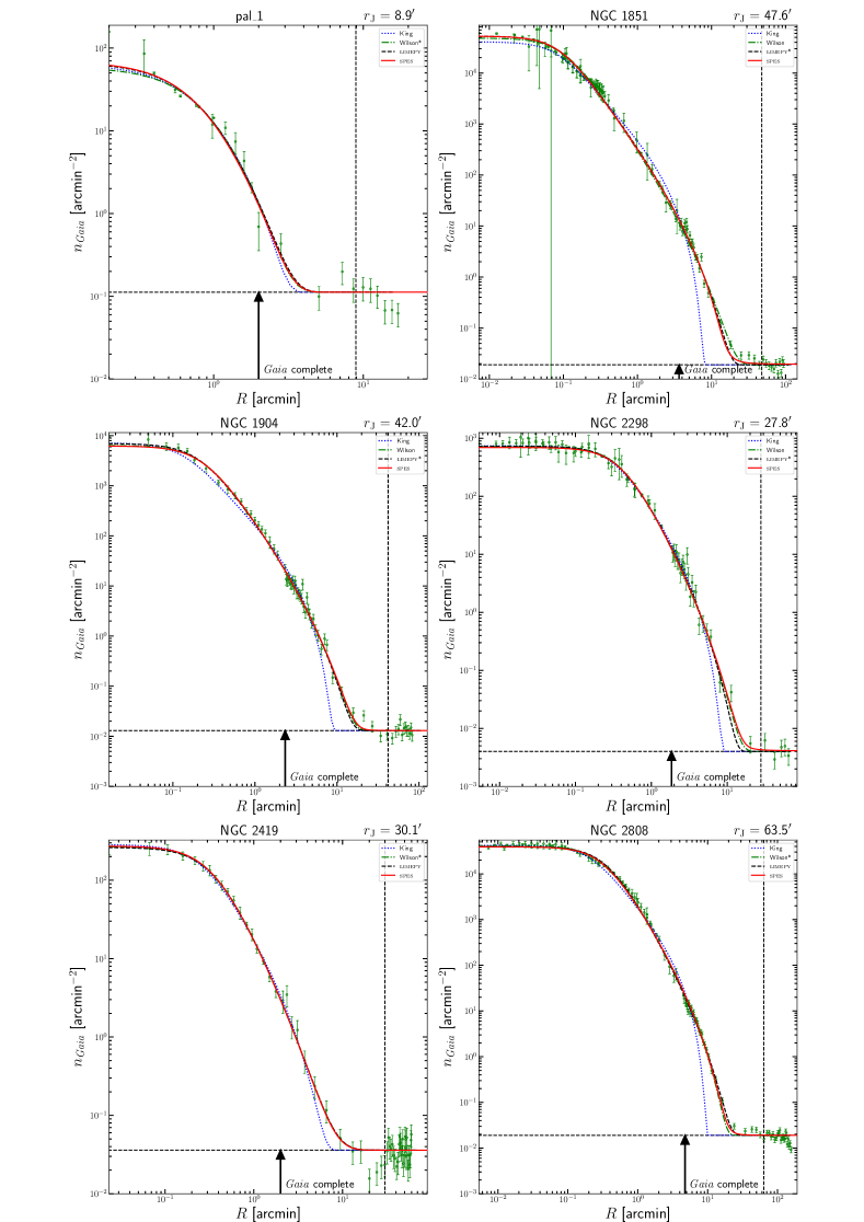
Figure 19: Figure 18 continued.

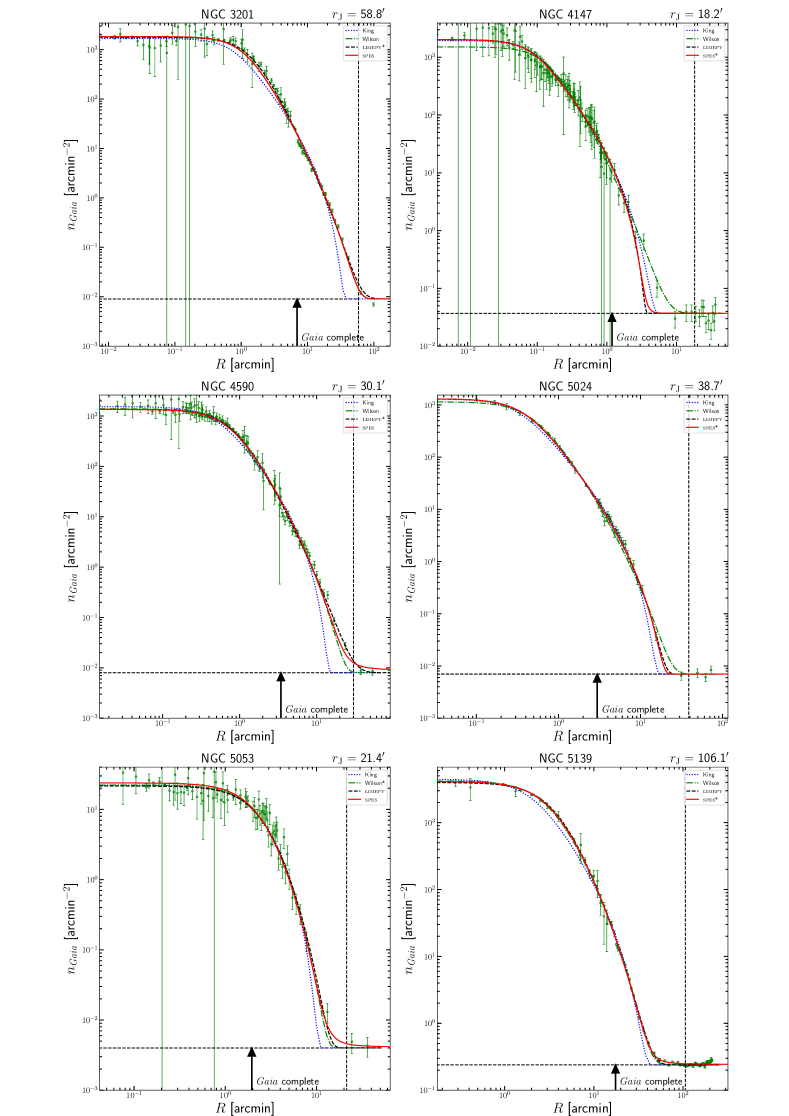
Figure 20: Figure 18 continued.

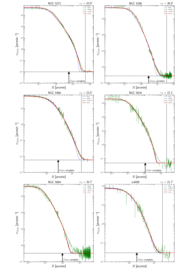
Figure 21: Figure 18 continued.

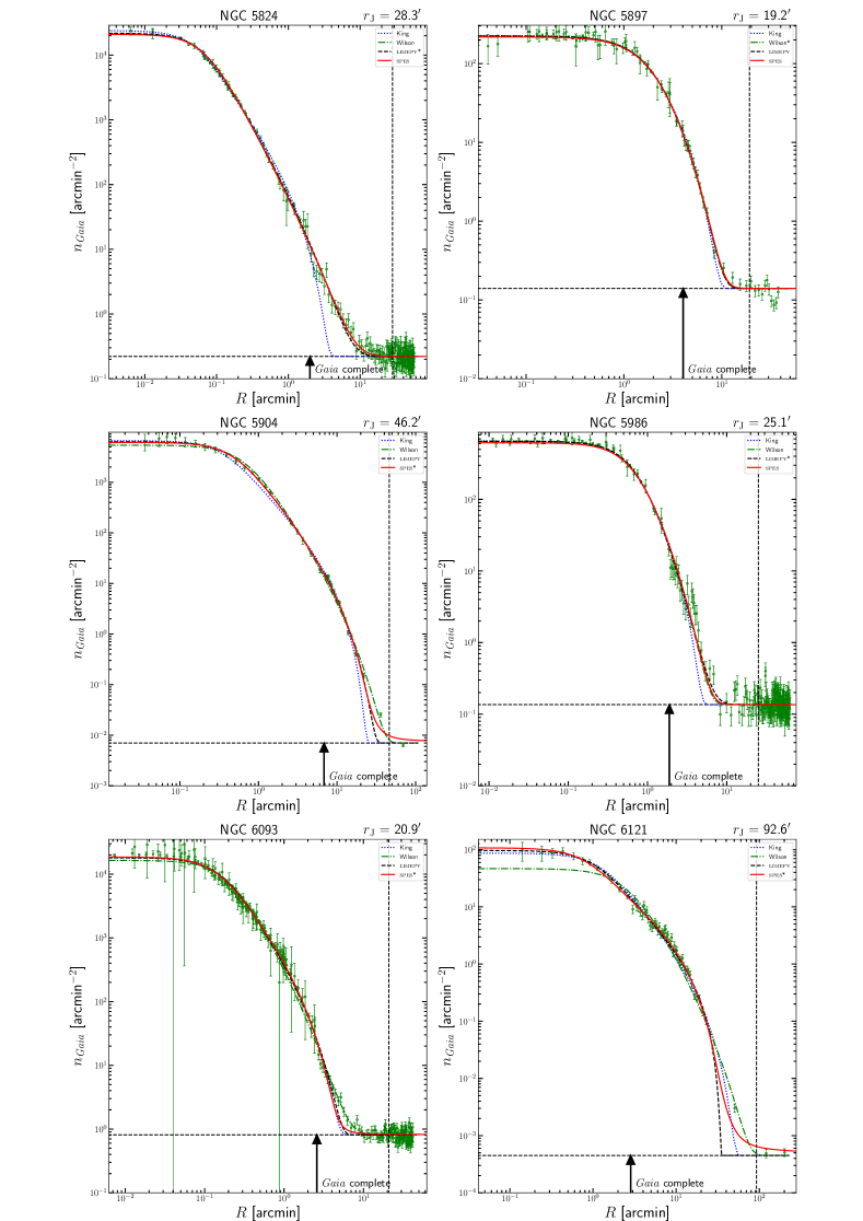
Figure 22: Figure 18 continued.

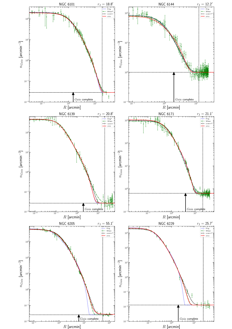
Figure 23: Figure 18 continued.

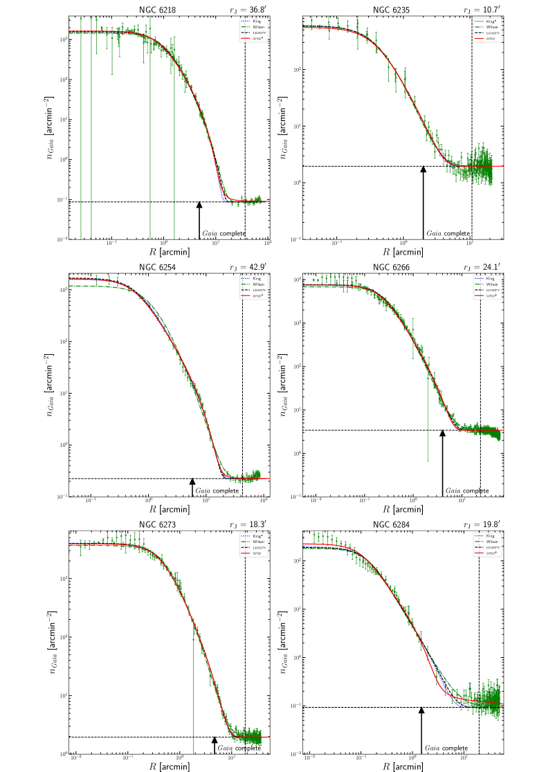
Figure 24: Figure 18 continued.

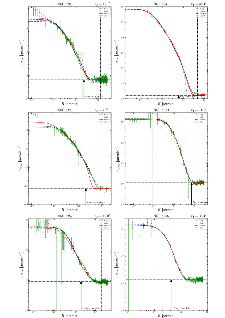
Figure 25: Figure 18 continued.

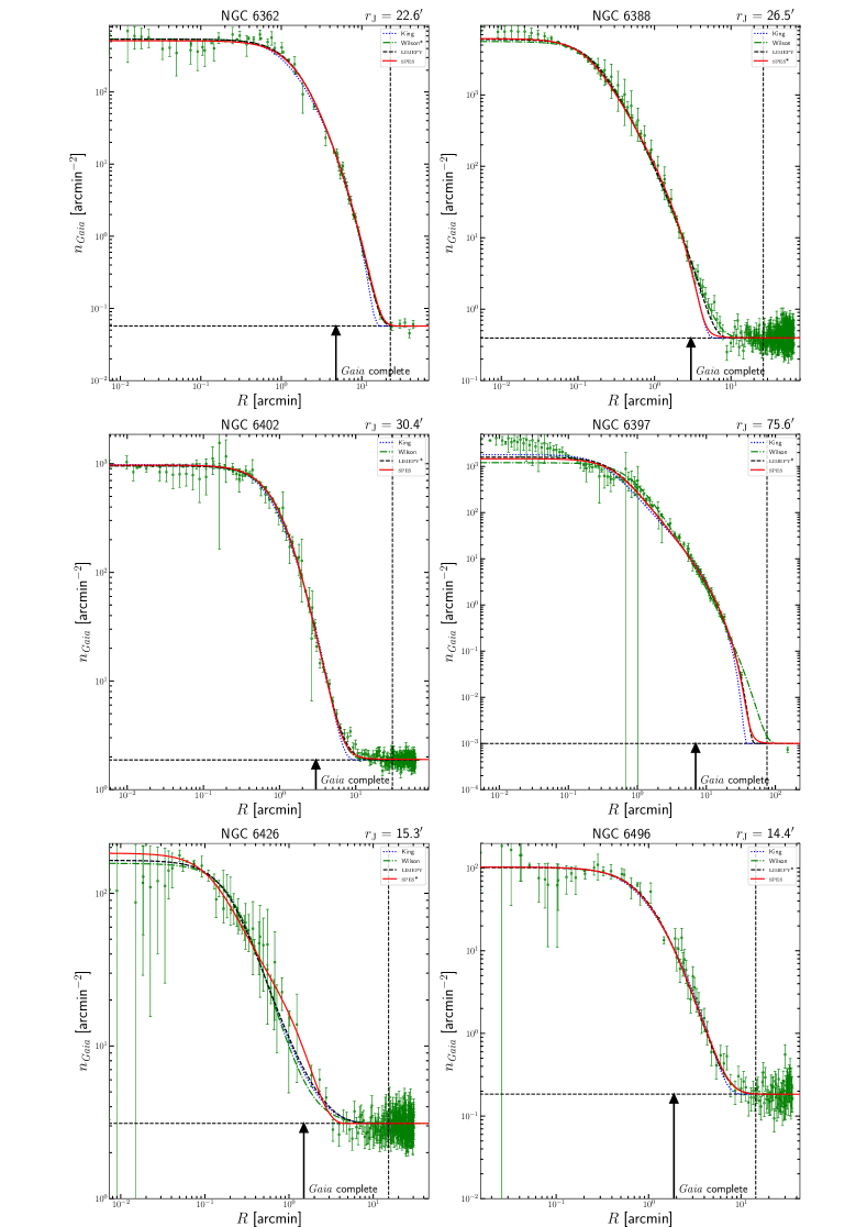
Figure 26: Figure 18 continued.

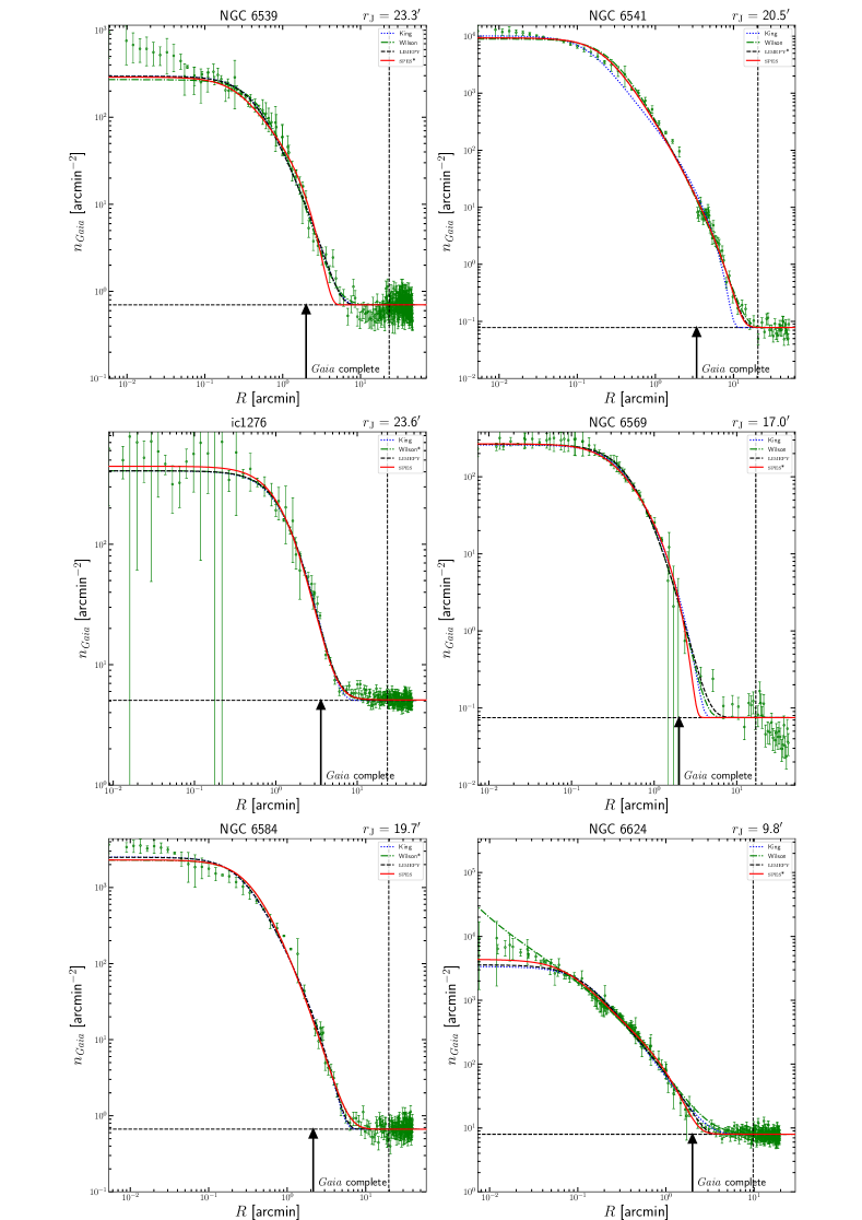
Figure 27: Figure 18 continued.

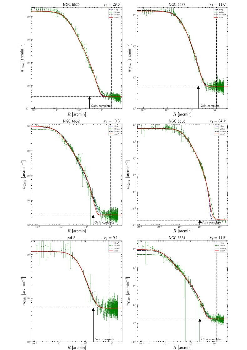
Figure 28: Figure 18 continued.

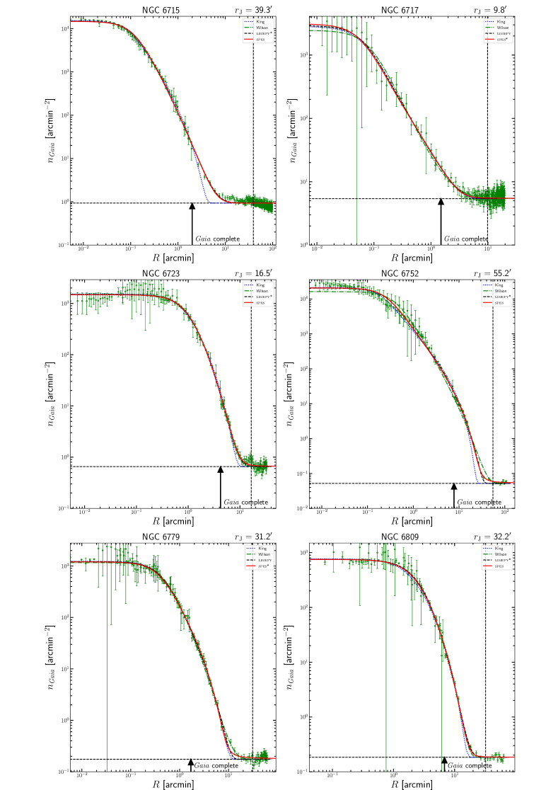
Figure 29: Figure 18 continued.

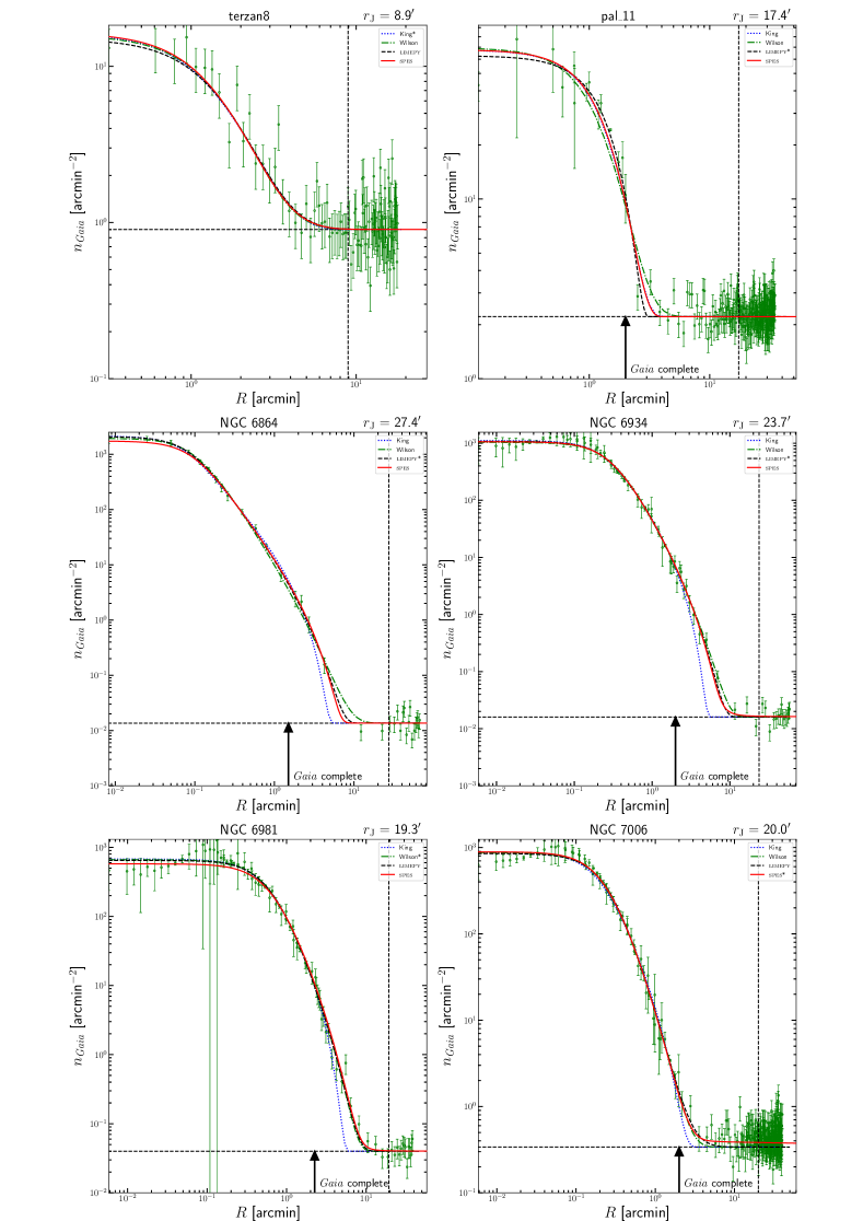
Figure 30: Figure 18 continued.

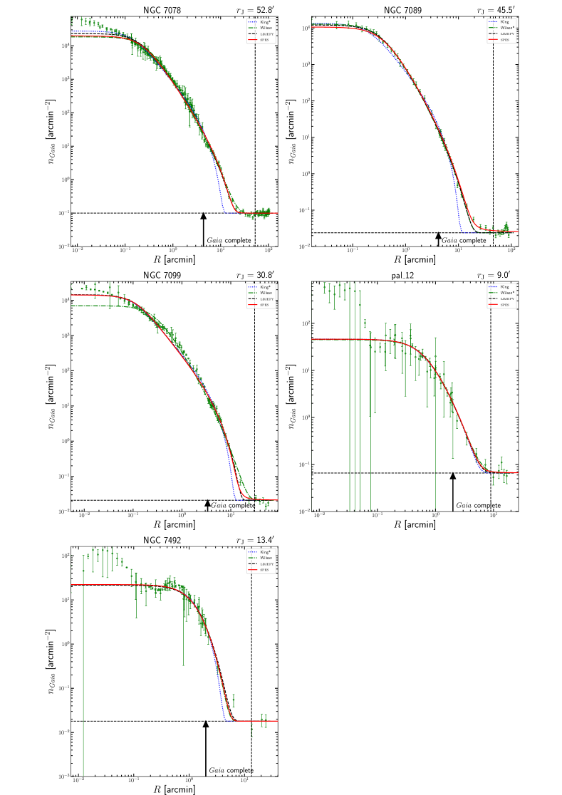
Figure 31: Figure 18 continued.

Appendix B GC profile fit parameters

Table 1: Best-fit parameters of limepy and spes models fit to 81 GCs following the procedure outlined in section 5.

	King		Wilson		limepy				spes
id	$W$	$r_{\mathrm{t}}$	$W$	$r_{\mathrm{t}}$	$W$	$g$	$r_{\mathrm{h}}$	$r_{\mathrm{t}}$	$W$	$\eta$	log10(1-B)	$r_{\mathrm{h}}$	$r_{\mathrm{t}}$	log10($f_{\mathrm{PE}}$)	$r_{\mathrm{tie}}$	BG lev	Mlow
		(pc)		(pc)			(pc)	(pc)				(pc)	(pc)		(arcmin)	(arcmin-2)	(M⊙)
ngc104	8.58$\pm$0.02	52.49$\pm$0.48	7.05$\pm$0.03	200.91$\pm$6.70	8.30$\pm$0.08	1.33$\pm$0.05	5.18$\pm$0.16	72.96$\pm$4.25	8.12$\pm$0.10	0.15$\pm$0.02	-1.82$\pm$0.18	5.20$\pm$0.17	57.33$\pm$3.24	-2.36$\pm$0.36	13.28	0.08	0.60
ngc288	4.60$\pm$0.04	46.31$\pm$0.47	3.47$\pm$0.07	74.14$\pm$1.54	1.73$\pm$0.89	2.69$\pm$0.23	9.11$\pm$0.07	116.40$\pm$19.83	3.28$\pm$0.17	0.24$\pm$0.01	-2.43$\pm$0.31	9.16$\pm$0.10	60.04$\pm$6.43	-2.31$\pm$0.22	4.05	0.01	0.74
ngc362	7.93$\pm$0.03	26.08$\pm$0.42	6.72$\pm$0.01	82.59$\pm$0.98	6.73$\pm$0.06	1.99$\pm$0.03	2.03$\pm$0.03	81.68$\pm$5.78	6.71$\pm$0.02	0.10$\pm$0.06	-4.31$\pm$1.55	2.03$\pm$0.02	80.02$\pm$4.44	-4.88$\pm$1.31	4.54	0.08	0.70
ngc1261	6.80$\pm$0.17	37.81$\pm$1.81	5.09$\pm$0.03	61.86$\pm$1.22	3.63$\pm$0.41	2.82$\pm$0.12	4.33$\pm$0.07	220.34$\pm$62.94	4.99$\pm$0.10	0.23$\pm$0.01	-2.59$\pm$0.22	4.45$\pm$0.04	51.51$\pm$4.51	-2.59$\pm$0.15	2.41	0.01	0.81
pal_1	3.36$\pm$0.67	12.97$\pm$1.13	1.44$\pm$0.80	18.67$\pm$1.83	2.42$\pm$1.80	1.92$\pm$0.78	3.21$\pm$0.22	19.67$\pm$10.55	2.17$\pm$1.07	0.18$\pm$0.13	-7.60$\pm$1.83	3.25$\pm$0.18	19.59$\pm$3.66	-4.48$\pm$1.75	2.00	0.11	0.76
ngc1851	8.37$\pm$0.07	31.92$\pm$0.64	7.28$\pm$0.01	161.34$\pm$2.94	7.64$\pm$0.06	1.85$\pm$0.02	2.51$\pm$0.05	109.26$\pm$7.53	7.46$\pm$0.05	0.13$\pm$0.01	-2.64$\pm$0.13	2.43$\pm$0.06	62.13$\pm$5.11	-2.33$\pm$0.13	3.64	0.02	0.78
ngc1904	7.93$\pm$0.11	38.32$\pm$1.01	6.56$\pm$0.03	112.90$\pm$2.82	6.79$\pm$0.20	1.89$\pm$0.09	3.20$\pm$0.10	97.22$\pm$13.76	6.57$\pm$0.07	0.13$\pm$0.08	-3.94$\pm$1.69	3.17$\pm$0.12	108.73$\pm$10.38	-4.70$\pm$1.40	2.33	0.01	0.74
ngc2298	6.76$\pm$0.04	30.05$\pm$0.62	6.08$\pm$0.04	82.20$\pm$3.04	6.35$\pm$0.17	1.75$\pm$0.16	3.49$\pm$0.08	60.05$\pm$11.80	6.08$\pm$0.08	0.19$\pm$0.11	-3.56$\pm$1.74	3.38$\pm$0.06	80.41$\pm$6.89	-4.69$\pm$1.81	1.84	0.01	0.71
ngc2419	6.82$\pm$0.10	209.46$\pm$10.30	6.24$\pm$0.08	671.82$\pm$50.93	6.15$\pm$0.31	2.04$\pm$0.18	24.50$\pm$1.13	704.85$\pm$236.03	6.22$\pm$0.16	0.17$\pm$0.13	-4.36$\pm$1.53	24.81$\pm$1.00	644.64$\pm$107.45	-5.46$\pm$1.56	2.00	0.04	0.77
ngc2808	7.44$\pm$0.04	28.91$\pm$0.43	6.32$\pm$0.01	74.66$\pm$0.84	5.89$\pm$0.08	2.22$\pm$0.03	2.48$\pm$0.02	100.06$\pm$6.57	6.28$\pm$0.03	0.13$\pm$0.01	-3.43$\pm$0.28	2.56$\pm$0.02	65.42$\pm$4.09	-3.35$\pm$0.31	4.75	0.02	0.73
ngc3201	7.45$\pm$0.08	57.10$\pm$1.97	6.42$\pm$0.02	163.67$\pm$3.88	5.75$\pm$0.19	2.30$\pm$0.07	4.98$\pm$0.08	249.11$\pm$34.88	6.42$\pm$0.05	0.16$\pm$0.12	-5.42$\pm$1.30	5.20$\pm$0.09	161.62$\pm$8.25	-5.45$\pm$1.18	6.95	0.01	0.60
ngc4147	7.63$\pm$0.03	32.56$\pm$0.63	6.71$\pm$0.05	127.58$\pm$8.21	7.60$\pm$0.08	0.60$\pm$0.17	3.25$\pm$0.10	21.93$\pm$3.58	7.90$\pm$0.09	0.23$\pm$0.05	-0.97$\pm$0.20	3.22$\pm$0.08	21.60$\pm$1.65	-2.07$\pm$0.40	1.18	0.03	0.78
ngc4590	6.79$\pm$0.04	50.77$\pm$1.15	5.84$\pm$0.03	122.02$\pm$2.90	5.17$\pm$0.08	2.46$\pm$0.04	5.74$\pm$0.05	295.80$\pm$42.45	5.74$\pm$0.06	0.22$\pm$0.01	-2.63$\pm$0.17	5.86$\pm$0.06	94.03$\pm$7.56	-2.53$\pm$0.12	3.44	0.01	0.72
ngc5024	7.53$\pm$0.05	92.82$\pm$1.84	6.34$\pm$0.03	242.61$\pm$5.56	7.04$\pm$0.10	1.53$\pm$0.07	8.92$\pm$0.21	145.10$\pm$10.60	6.81$\pm$0.10	0.09$\pm$0.04	-2.49$\pm$0.30	8.83$\pm$0.22	118.76$\pm$7.27	-3.43$\pm$0.52	2.96	0.01	0.77
ngc5053	2.96$\pm$0.19	59.38$\pm$2.03	1.58$\pm$0.53	91.51$\pm$7.37	1.07$\pm$0.71	2.24$\pm$0.24	16.11$\pm$0.29	106.30$\pm$19.69	1.50$\pm$0.59	0.20$\pm$0.05	-2.99$\pm$0.67	15.95$\pm$0.39	77.32$\pm$16.51	-2.20$\pm$0.66	1.95	0.01	0.77
ngc5139	6.25$\pm$0.02	70.25$\pm$0.56	4.82$\pm$0.01	114.30$\pm$0.85	3.97$\pm$0.26	2.33$\pm$0.09	9.34$\pm$0.07	137.30$\pm$8.62	4.57$\pm$0.07	0.25$\pm$0.01	-2.83$\pm$0.27	9.36$\pm$0.06	97.07$\pm$7.23	-2.67$\pm$0.17	17.51	0.24	0.60
ngc5272	8.10$\pm$0.07	77.55$\pm$1.06	6.48$\pm$0.02	197.84$\pm$5.01	7.46$\pm$0.08	1.53$\pm$0.04	6.71$\pm$0.14	121.27$\pm$4.54	7.22$\pm$0.09	0.20$\pm$0.01	-1.75$\pm$0.07	6.64$\pm$0.13	79.92$\pm$2.97	-2.06$\pm$0.06	5.71	0.01	0.72
ngc5286	7.52$\pm$0.04	37.78$\pm$0.79	6.53$\pm$0.02	123.14$\pm$3.24	6.33$\pm$0.12	2.14$\pm$0.07	3.52$\pm$0.05	172.84$\pm$33.08	6.42$\pm$0.05	0.20$\pm$0.01	-2.80$\pm$0.33	3.57$\pm$0.04	86.73$\pm$14.06	-2.32$\pm$0.19	2.80	0.28	0.73
ngc5466	6.01$\pm$0.16	103.67$\pm$5.27	5.03$\pm$0.10	197.77$\pm$9.20	3.78$\pm$0.73	2.62$\pm$0.25	14.45$\pm$0.37	363.35$\pm$123.16	5.00$\pm$0.22	0.24$\pm$0.12	-2.98$\pm$1.83	14.68$\pm$0.40	189.98$\pm$23.10	-4.21$\pm$1.97	2.85	0.01	0.76
ngc5634	7.88$\pm$0.04	49.30$\pm$0.94	6.82$\pm$0.05	192.08$\pm$11.31	7.86$\pm$0.08	1.06$\pm$0.12	5.17$\pm$0.17	52.80$\pm$7.25	7.88$\pm$0.12	0.17$\pm$0.04	-1.45$\pm$0.24	5.11$\pm$0.21	43.99$\pm$4.21	-2.38$\pm$0.42	1.09	0.05	0.76
ngc5694	7.54$\pm$0.02	36.49$\pm$0.25	7.28$\pm$0.03	344.18$\pm$21.19	7.55$\pm$0.05	1.07$\pm$0.19	3.95$\pm$0.11	39.80$\pm$9.69	7.47$\pm$0.10	0.26$\pm$0.05	-1.13$\pm$0.29	3.88$\pm$0.05	30.37$\pm$2.44	-1.81$\pm$0.52	0.95	0.34	0.76
ic4499	5.71$\pm$0.10	78.08$\pm$2.77	4.90$\pm$0.12	154.70$\pm$9.10	4.93$\pm$0.54	1.93$\pm$0.35	12.07$\pm$0.31	142.30$\pm$45.01	4.88$\pm$0.28	0.19$\pm$0.09	-2.78$\pm$1.56	12.09$\pm$0.29	137.66$\pm$28.96	-3.79$\pm$1.79	2.01	0.03	0.76
ngc5824	8.17$\pm$0.02	41.55$\pm$0.49	7.46$\pm$0.02	381.98$\pm$11.92	7.63$\pm$0.07	1.88$\pm$0.04	4.61$\pm$0.14	230.01$\pm$43.68	7.45$\pm$0.03	0.07$\pm$0.02	-4.72$\pm$0.76	4.56$\pm$0.11	348.56$\pm$58.23	-3.76$\pm$0.75	2.00	0.22	0.76
ngc5897	3.79$\pm$0.04	41.94$\pm$0.45	2.34$\pm$0.05	62.22$\pm$0.79	2.36$\pm$0.68	1.99$\pm$0.27	9.72$\pm$0.09	62.44$\pm$8.28	2.32$\pm$0.16	0.19$\pm$0.10	-3.48$\pm$1.74	9.69$\pm$0.08	60.95$\pm$2.75	-4.57$\pm$1.63	4.03	0.14	0.73
ngc5904	7.93$\pm$0.05	56.56$\pm$0.91	6.40$\pm$0.03	143.70$\pm$3.69	7.23$\pm$0.17	1.50$\pm$0.09	5.06$\pm$0.15	82.84$\pm$7.04	6.98$\pm$0.15	0.21$\pm$0.01	-1.70$\pm$0.09	5.01$\pm$0.14	57.36$\pm$2.69	-2.07$\pm$0.07	6.82	0.01	0.68
ngc5986	4.75$\pm$0.09	17.62$\pm$0.48	4.14$\pm$0.07	33.77$\pm$1.02	3.01$\pm$0.42	2.61$\pm$0.12	3.42$\pm$0.05	57.49$\pm$7.16	4.06$\pm$0.18	0.20$\pm$0.04	-2.68$\pm$0.54	3.46$\pm$0.04	29.69$\pm$3.17	-2.97$\pm$0.70	1.88	0.14	0.72
ngc6093	7.13$\pm$0.01	18.40$\pm$0.11	6.33$\pm$0.02	54.29$\pm$1.14	7.07$\pm$0.05	1.18$\pm$0.09	2.04$\pm$0.02	21.32$\pm$1.71	7.26$\pm$0.12	0.28$\pm$0.02	-0.94$\pm$0.11	2.11$\pm$0.02	14.25$\pm$0.76	-1.77$\pm$0.10	2.59	0.81	0.70
ngc6121	7.29$\pm$0.10	37.50$\pm$0.88	5.80$\pm$0.11	83.58$\pm$3.96	7.64$\pm$0.13	0.18$\pm$0.07	4.47$\pm$0.09	22.75$\pm$0.80	9.09$\pm$0.23	0.34$\pm$0.01	-0.22$\pm$0.09	4.77$\pm$0.10	22.70$\pm$0.66	-1.58$\pm$0.03	2.83	0.00	0.50
ngc6101	6.28$\pm$0.04	91.06$\pm$1.72	5.34$\pm$0.05	181.73$\pm$5.63	5.85$\pm$0.63	1.56$\pm$0.51	12.01$\pm$0.42	129.88$\pm$67.62	5.84$\pm$0.24	0.17$\pm$0.05	-1.72$\pm$0.33	12.11$\pm$0.27	95.13$\pm$8.75	-2.65$\pm$0.42	3.29	0.03	0.76
ngc6144	5.61$\pm$0.12	35.76$\pm$1.56	4.69$\pm$0.22	66.49$\pm$6.31	5.78$\pm$0.20	0.22$\pm$0.14	5.92$\pm$0.22	25.12$\pm$2.28	9.24$\pm$0.68	0.13$\pm$0.04	-0.15$\pm$0.17	6.20$\pm$0.20	23.85$\pm$1.31	-3.62$\pm$0.64	2.00	1.01	0.70
ngc6139	7.92$\pm$0.04	29.31$\pm$0.76	7.26$\pm$0.05	214.83$\pm$19.61	7.92$\pm$0.09	1.30$\pm$0.14	3.24$\pm$0.18	44.81$\pm$10.06	7.89$\pm$0.16	0.24$\pm$0.06	-1.20$\pm$0.33	3.02$\pm$0.23	24.69$\pm$6.54	-1.85$\pm$0.41	2.00	0.03	0.76
ngc6171	6.63$\pm$0.02	29.54$\pm$0.33	5.83$\pm$0.05	71.03$\pm$2.61	6.76$\pm$0.05	0.43$\pm$0.15	3.88$\pm$0.06	21.39$\pm$1.77	7.39$\pm$0.14	0.27$\pm$0.04	-0.73$\pm$0.14	3.95$\pm$0.06	21.97$\pm$0.98	-1.96$\pm$0.22	3.92	0.64	0.65
ngc6205	6.55$\pm$0.06	35.69$\pm$0.69	5.49$\pm$0.03	71.99$\pm$1.14	4.11$\pm$0.18	2.63$\pm$0.06	4.18$\pm$0.03	138.92$\pm$14.71	5.34$\pm$0.06	0.21$\pm$0.01	-2.67$\pm$0.17	4.27$\pm$0.04	56.90$\pm$3.74	-2.68$\pm$0.13	6.12	0.03	0.67
ngc6229	6.59$\pm$0.09	36.49$\pm$0.87	5.86$\pm$0.08	92.57$\pm$5.32	5.08$\pm$0.42	2.51$\pm$0.15	4.36$\pm$0.17	255.37$\pm$111.96	5.85$\pm$0.18	0.19$\pm$0.13	-7.94$\pm$1.68	4.40$\pm$0.16	89.84$\pm$10.94	-5.35$\pm$1.65	2.00	0.01	0.77
ngc6218	6.00$\pm$0.02	29.35$\pm$0.23	4.90$\pm$0.03	52.95$\pm$0.81	5.73$\pm$0.13	1.37$\pm$0.12	4.24$\pm$0.04	36.28$\pm$2.65	6.20$\pm$0.22	0.32$\pm$0.01	-0.78$\pm$0.13	4.34$\pm$0.04	22.94$\pm$0.94	-1.71$\pm$0.05	4.83	0.09	0.64
ngc6235	6.27$\pm$0.07	26.27$\pm$0.93	5.78$\pm$0.09	70.73$\pm$5.49	6.22$\pm$0.17	1.25$\pm$0.25	3.61$\pm$0.12	32.18$\pm$6.79	6.11$\pm$0.20	0.18$\pm$0.05	-1.53$\pm$0.29	3.60$\pm$0.12	26.59$\pm$3.64	-2.56$\pm$0.48	1.99	1.96	0.73
ngc6254	7.06$\pm$0.02	38.47$\pm$0.41	5.75$\pm$0.07	81.66$\pm$2.70	7.27$\pm$0.14	0.82$\pm$0.10	4.53$\pm$0.12	34.80$\pm$1.87	7.51$\pm$0.23	0.30$\pm$0.04	-0.82$\pm$0.18	4.61$\pm$0.12	29.50$\pm$2.09	-1.74$\pm$0.24	5.78	0.23	0.60
ngc6266	7.48$\pm$0.05	22.87$\pm$0.40	6.78$\pm$0.04	102.01$\pm$5.82	7.39$\pm$0.12	1.24$\pm$0.15	2.43$\pm$0.06	28.81$\pm$4.93	7.58$\pm$0.26	0.21$\pm$0.05	-1.24$\pm$0.28	2.48$\pm$0.08	19.47$\pm$2.13	-2.20$\pm$0.47	4.00	3.40	0.70
ngc6273	6.80$\pm$0.01	35.04$\pm$0.27	5.97$\pm$0.03	88.89$\pm$2.10	6.75$\pm$0.05	1.10$\pm$0.07	4.22$\pm$0.04	37.70$\pm$2.11	6.66$\pm$0.09	0.26$\pm$0.03	-1.15$\pm$0.15	4.22$\pm$0.03	30.51$\pm$1.89	-1.92$\pm$0.24	4.70	1.95	0.68
ngc6284	8.31$\pm$0.09	54.13$\pm$2.30	8.40$\pm$0.09	1397.22$\pm$41.25	8.37$\pm$0.20	1.26$\pm$0.27	6.68$\pm$1.14	83.73$\pm$44.86	8.41$\pm$0.20	0.49$\pm$0.01	-0.12$\pm$0.06	3.79$\pm$0.18	16.28$\pm$0.93	-1.05$\pm$0.02	1.50	0.09	0.76
ngc6293	7.29$\pm$0.07	21.19$\pm$0.57	6.67$\pm$0.08	90.04$\pm$9.38	7.51$\pm$0.12	0.15$\pm$0.05	2.44$\pm$0.08	12.30$\pm$0.56	9.81$\pm$0.15	0.24$\pm$0.04	-0.16$\pm$0.16	2.55$\pm$0.05	11.60$\pm$0.42	-2.26$\pm$0.32	2.20	6.53	0.71
ngc6341	7.47$\pm$0.12	23.29$\pm$1.40	6.80$\pm$0.13	107.11$\pm$19.23	6.99$\pm$0.20	1.83$\pm$0.10	3.16$\pm$0.12	93.01$\pm$13.28	6.97$\pm$0.16	0.20$\pm$0.01	-1.90$\pm$0.15	3.21$\pm$0.13	45.36$\pm$4.00	-2.02$\pm$0.07	6.00	0.02	0.67
ngc6325	5.53$\pm$0.03	16.22$\pm$0.19	4.94$\pm$0.04	34.21$\pm$0.74	7.54$\pm$0.29	0.70$\pm$0.34	2.54$\pm$0.25	18.48$\pm$5.27	9.91$\pm$0.15	0.30$\pm$0.08	-0.01$\pm$0.23	2.14$\pm$0.17	9.69$\pm$1.02	-1.82$\pm$0.58	2.00	0.07	0.77
ngc6333	8.05$\pm$0.10	40.27$\pm$0.79	6.68$\pm$0.03	118.47$\pm$3.31	4.75$\pm$0.16	2.13$\pm$0.10	2.62$\pm$0.02	38.76$\pm$4.37	4.91$\pm$0.09	0.14$\pm$0.05	-2.99$\pm$0.77	2.62$\pm$0.02	30.94$\pm$3.13	-3.80$\pm$0.89	7.02	11.56	0.68
ngc6352	8.13$\pm$0.07	50.21$\pm$1.90	7.76$\pm$0.10	741.42$\pm$116.58	8.15$\pm$0.12	0.16$\pm$0.06	5.19$\pm$0.31	25.57$\pm$1.74	10.73$\pm$0.43	0.17$\pm$0.05	-0.25$\pm$0.24	5.03$\pm$0.21	21.82$\pm$1.32	-2.92$\pm$0.55	2.00	9.23	0.66
ngc6366	4.83$\pm$0.09	21.00$\pm$0.51	3.70$\pm$0.12	34.80$\pm$1.31	2.24$\pm$0.96	2.62$\pm$0.26	4.07$\pm$0.06	53.13$\pm$13.01	3.73$\pm$0.27	0.24$\pm$0.14	-4.07$\pm$1.61	4.07$\pm$0.07	34.68$\pm$3.01	-5.13$\pm$1.74	4.24	1.38	0.65
ngc6362	5.64$\pm$0.06	38.31$\pm$0.61	4.47$\pm$0.06	63.86$\pm$1.32	4.45$\pm$0.38	1.99$\pm$0.19	5.91$\pm$0.07	63.34$\pm$8.01	4.44$\pm$0.13	0.16$\pm$0.07	-2.95$\pm$1.28	5.90$\pm$0.07	58.36$\pm$6.76	-3.77$\pm$1.35	4.77	0.06	0.68
ngc6388	7.30$\pm$0.03	17.98$\pm$0.18	6.58$\pm$0.03	67.62$\pm$2.27	7.04$\pm$0.12	1.57$\pm$0.14	1.93$\pm$0.03	33.53$\pm$6.53	7.32$\pm$0.22	0.26$\pm$0.03	-1.06$\pm$0.27	1.96$\pm$0.04	14.56$\pm$2.33	-1.84$\pm$0.22	2.00	0.39	0.79
ngc6402	5.41$\pm$0.07	28.40$\pm$0.72	4.57$\pm$0.07	53.35$\pm$1.65	3.74$\pm$0.23	2.58$\pm$0.09	4.74$\pm$0.04	103.90$\pm$16.50	4.29$\pm$0.14	0.30$\pm$0.01	-2.13$\pm$0.19	4.70$\pm$0.05	37.73$\pm$4.03	-2.03$\pm$0.14	3.00	1.88	0.74
ngc6397	8.65$\pm$0.10	32.16$\pm$0.45	6.75$\pm$0.03	103.67$\pm$3.87	8.06$\pm$0.18	1.32$\pm$0.07	3.06$\pm$0.15	43.00$\pm$3.08	7.90$\pm$0.23	0.17$\pm$0.03	-1.72$\pm$0.23	3.06$\pm$0.16	33.61$\pm$2.45	-2.22$\pm$0.26	7.00	0.01	0.50
ngc6426	7.84$\pm$0.14	84.37$\pm$7.36	7.21$\pm$0.16	553.74$\pm$168.71	7.91$\pm$0.29	0.53$\pm$0.35	9.32$\pm$1.65	58.48$\pm$20.72	11.73$\pm$0.64	0.11$\pm$0.04	-0.06$\pm$0.17	8.06$\pm$0.71	30.42$\pm$3.91	-3.88$\pm$0.62	1.50	3.11	0.75
ngc6496	5.43$\pm$0.13	35.15$\pm$1.54	4.78$\pm$0.14	71.00$\pm$5.08	4.09$\pm$0.85	2.32$\pm$0.31	5.70$\pm$0.22	86.35$\pm$25.43	4.74$\pm$0.30	0.23$\pm$0.13	-3.56$\pm$1.75	5.83$\pm$0.19	67.95$\pm$10.05	-4.89$\pm$1.84	1.87	0.18	0.82
ngc6539	6.40$\pm$0.12	23.28$\pm$1.05	5.52$\pm$0.13	51.01$\pm$4.43	6.47$\pm$0.25	0.76$\pm$0.37	3.12$\pm$0.13	20.25$\pm$4.99	9.85$\pm$0.94	0.13$\pm$0.05	-0.15$\pm$0.20	3.12$\pm$0.10	12.49$\pm$1.06	-3.56$\pm$0.76	2.00	0.70	0.82
ngc6541	8.20$\pm$0.10	25.98$\pm$0.51	6.55$\pm$0.03	69.03$\pm$1.94	7.06$\pm$0.19	1.73$\pm$0.09	2.09$\pm$0.07	50.09$\pm$5.82	6.80$\pm$0.16	0.14$\pm$0.03	-2.40$\pm$0.41	2.04$\pm$0.05	35.68$\pm$5.10	-2.64$\pm$0.66	3.36	0.08	0.66
ic1276	4.47$\pm$0.15	16.63$\pm$0.50	3.89$\pm$0.22	31.41$\pm$1.93	2.93$\pm$0.84	2.58$\pm$0.31	3.51$\pm$0.08	52.86$\pm$19.89	3.71$\pm$0.49	0.32$\pm$0.07	-2.16$\pm$1.40	3.48$\pm$0.07	23.28$\pm$8.61	-1.92$\pm$1.11	3.57	5.06	0.78
ngc6569	5.21$\pm$0.14	15.72$\pm$0.84	4.20$\pm$0.24	25.62$\pm$2.33	3.64$\pm$0.91	2.43$\pm$0.33	2.58$\pm$0.11	39.43$\pm$14.56	6.98$\pm$0.44	0.21$\pm$0.05	-0.49$\pm$0.28	2.81$\pm$0.06	11.59$\pm$0.75	-2.52$\pm$0.37	2.00	0.08	0.81
ngc6584	6.75$\pm$0.06	30.82$\pm$0.66	5.80$\pm$0.07	71.48$\pm$3.40	6.66$\pm$0.24	1.15$\pm$0.26	3.75$\pm$0.11	33.95$\pm$6.27	5.81$\pm$0.16	0.21$\pm$0.14	-5.81$\pm$1.45	3.54$\pm$0.07	71.08$\pm$7.44	-5.68$\pm$1.57	2.14	0.67	0.76
ngc6624	7.75$\pm$0.03	17.73$\pm$0.34	15.43$\pm$0.11	85.41$\pm$2.11	7.66$\pm$0.09	0.16$\pm$0.14	1.72$\pm$0.07	8.63$\pm$1.07	9.39$\pm$0.12	0.37$\pm$0.06	-0.00$\pm$0.22	1.66$\pm$0.01	7.29$\pm$0.33	-1.54$\pm$0.39	2.00	7.97	0.80
ngc6626	7.70$\pm$0.02	22.81$\pm$0.30	6.98$\pm$0.03	115.62$\pm$6.25	7.65$\pm$0.07	1.17$\pm$0.12	2.38$\pm$0.06	26.99$\pm$3.60	7.65$\pm$0.13	0.24$\pm$0.03	-1.20$\pm$0.20	2.39$\pm$0.06	19.26$\pm$1.80	-1.91$\pm$0.29	3.00	0.33	0.69
ngc6637	5.99$\pm$0.04	16.47$\pm$0.34	5.36$\pm$0.08	36.87$\pm$1.82	6.02$\pm$0.11	0.76$\pm$0.31	2.43$\pm$0.05	14.30$\pm$2.76	6.56$\pm$0.28	0.25$\pm$0.05	-0.75$\pm$0.25	2.44$\pm$0.04	12.41$\pm$0.93	-2.22$\pm$0.42	2.00	5.28	0.75
ngc6652	7.83$\pm$0.04	16.72$\pm$0.25	6.92$\pm$0.04	78.74$\pm$4.94	7.92$\pm$0.06	0.46$\pm$0.16	1.78$\pm$0.03	10.86$\pm$1.25	8.99$\pm$0.14	0.25$\pm$0.03	-0.55$\pm$0.22	1.79$\pm$0.03	9.58$\pm$0.44	-2.01$\pm$0.48	1.93	2.58	0.75
ngc6656	6.74$\pm$0.01	36.07$\pm$0.21	5.67$\pm$0.03	74.49$\pm$1.34	6.57$\pm$0.05	1.19$\pm$0.05	4.31$\pm$0.03	40.12$\pm$1.42	6.36$\pm$0.06	0.24$\pm$0.01	-1.34$\pm$0.06	4.28$\pm$0.04	33.03$\pm$0.83	-2.05$\pm$0.05	10.00	0.01	0.50
pal_8	5.21$\pm$0.20	26.13$\pm$2.19	4.56$\pm$0.26	50.01$\pm$6.80	5.12$\pm$0.47	1.34$\pm$0.42	4.65$\pm$0.34	32.50$\pm$9.03	6.19$\pm$0.95	0.16$\pm$0.07	-1.07$\pm$0.59	4.66$\pm$0.33	21.62$\pm$4.68	-3.03$\pm$0.71	2.00	5.96	0.86
ngc6681	8.27$\pm$0.04	23.77$\pm$0.37	7.03$\pm$0.05	121.76$\pm$8.02	8.33$\pm$0.12	0.87$\pm$0.10	2.53$\pm$0.07	21.09$\pm$2.14	8.88$\pm$0.21	0.28$\pm$0.07	-0.77$\pm$0.36	2.58$\pm$0.08	15.17$\pm$1.74	-1.65$\pm$0.71	2.44	1.75	0.69
ngc6715	7.56$\pm$0.07	41.06$\pm$1.33	7.06$\pm$0.03	255.76$\pm$12.88	6.99$\pm$0.10	2.06$\pm$0.06	4.54$\pm$0.16	345.99$\pm$137.41	7.04$\pm$0.06	0.09$\pm$0.04	-3.98$\pm$1.35	4.50$\pm$0.14	216.86$\pm$35.60	-3.41$\pm$0.98	2.00	0.93	0.80
ngc6717	9.02$\pm$0.15	19.50$\pm$0.88	8.29$\pm$0.16	358.05$\pm$28.63	8.88$\pm$0.35	1.34$\pm$0.26	2.47$\pm$0.32	30.60$\pm$14.39	8.88$\pm$0.44	0.34$\pm$0.11	-0.90$\pm$0.61	2.33$\pm$0.31	12.88$\pm$6.70	-1.18$\pm$0.66	1.50	5.41	0.70
ngc6723	5.39$\pm$0.05	28.69$\pm$0.37	4.56$\pm$0.03	52.76$\pm$0.79	4.14$\pm$0.21	2.28$\pm$0.13	4.68$\pm$0.04	67.66$\pm$9.50	4.35$\pm$0.09	0.27$\pm$0.01	-2.24$\pm$0.23	4.69$\pm$0.03	39.97$\pm$4.19	-2.21$\pm$0.17	4.20	0.65	0.70
ngc6752	8.87$\pm$0.04	32.19$\pm$0.31	7.00$\pm$0.02	119.23$\pm$3.16	8.20$\pm$0.08	1.46$\pm$0.03	3.03$\pm$0.06	52.37$\pm$2.14	7.97$\pm$0.09	0.19$\pm$0.01	-1.74$\pm$0.06	3.01$\pm$0.08	34.72$\pm$1.27	-1.93$\pm$0.05	7.78	0.05	0.55
ngc6779	6.92$\pm$0.03	37.86$\pm$0.47	6.22$\pm$0.03	112.33$\pm$3.75	6.82$\pm$0.10	1.25$\pm$0.16	4.41$\pm$0.07	46.46$\pm$6.73	6.95$\pm$0.15	0.34$\pm$0.01	-0.77$\pm$0.10	4.46$\pm$0.08	27.20$\pm$1.51	-1.56$\pm$0.04	1.70	0.18	0.70
ngc6809	4.64$\pm$0.05	29.55$\pm$0.32	2.96$\pm$0.04	42.10$\pm$0.37	0.82$\pm$0.59	2.64$\pm$0.12	5.79$\pm$0.03	56.51$\pm$3.73	2.90$\pm$0.10	0.23$\pm$0.12	-3.15$\pm$1.49	5.84$\pm$0.03	39.80$\pm$0.99	-2.82$\pm$1.63	6.83	0.18	0.60
terzan8	3.86$\pm$0.59	69.69$\pm$9.10	2.38$\pm$1.11	104.29$\pm$23.18	2.89$\pm$1.62	1.88$\pm$0.80	16.49$\pm$1.46	107.51$\pm$68.34	2.81$\pm$1.28	0.33$\pm$0.14	-6.98$\pm$2.12	16.53$\pm$1.52	112.97$\pm$37.24	-6.19$\pm$1.84	0.00	0.90	0.77
pal_11	0.18$\pm$0.08	16.38$\pm$0.29	0.21$\pm$0.10	29.34$\pm$0.72	0.27$\pm$0.18	0.16$\pm$0.07	5.83$\pm$0.13	12.10$\pm$0.41	1.29$\pm$1.53	0.04$\pm$0.05	-0.06$\pm$0.87	5.78$\pm$0.16	16.00$\pm$0.57	-4.42$\pm$2.69	2.00	2.22	0.83
ngc6864	8.02$\pm$0.08	34.77$\pm$1.36	7.05$\pm$0.04	165.56$\pm$11.52	7.60$\pm$0.21	1.61$\pm$0.15	3.34$\pm$0.22	74.72$\pm$20.26	7.41$\pm$0.21	0.12$\pm$0.04	-2.22$\pm$0.39	3.33$\pm$0.26	49.88$\pm$9.89	-2.87$\pm$0.59	1.02	0.16	0.77
ngc6934	6.33$\pm$0.03	26.12$\pm$0.32	6.03$\pm$0.03	88.01$\pm$2.66	6.22$\pm$0.09	1.76$\pm$0.13	3.71$\pm$0.06	61.21$\pm$12.27	5.98$\pm$0.07	0.23$\pm$0.04	-1.75$\pm$0.52	3.71$\pm$0.06	36.83$\pm$14.03	-2.13$\pm$0.47	2.00	0.02	0.78
ngc6981	5.27$\pm$0.06	30.55$\pm$0.61	4.83$\pm$0.05	67.95$\pm$1.59	4.52$\pm$0.28	2.18$\pm$0.17	5.40$\pm$0.08	77.95$\pm$14.00	4.68$\pm$0.13	0.23$\pm$0.04	-2.25$\pm$0.56	5.43$\pm$0.05	52.06$\pm$9.26	-2.60$\pm$0.54	2.25	0.04	0.79
ngc7006	5.87$\pm$0.09	40.10$\pm$1.01	5.27$\pm$0.04	89.69$\pm$2.46	4.52$\pm$0.23	2.58$\pm$0.10	5.92$\pm$0.08	238.71$\pm$67.80	5.15$\pm$0.12	0.38$\pm$0.05	-3.06$\pm$0.51	5.93$\pm$0.07	79.97$\pm$8.63	-2.22$\pm$0.25	2.00	0.34	0.77
ngc7078	8.19$\pm$0.03	39.57$\pm$0.40	6.87$\pm$0.01	163.72$\pm$3.08	7.53$\pm$0.08	1.67$\pm$0.04	3.75$\pm$0.06	93.65$\pm$6.12	7.16$\pm$0.08	0.14$\pm$0.02	-2.35$\pm$0.24	3.63$\pm$0.06	68.13$\pm$5.90	-2.51$\pm$0.34	4.37	0.10	0.71
ngc7089	7.60$\pm$0.09	40.18$\pm$0.75	6.32$\pm$0.02	98.82$\pm$1.76	6.26$\pm$0.18	2.01$\pm$0.08	3.47$\pm$0.08	98.56$\pm$10.28	6.19$\pm$0.08	0.19$\pm$0.01	-2.48$\pm$0.44	3.50$\pm$0.08	64.86$\pm$13.64	-2.52$\pm$0.26	4.19	0.02	0.74
ngc7099	8.67$\pm$0.07	31.35$\pm$0.33	6.75$\pm$0.04	107.86$\pm$4.27	8.36$\pm$0.12	1.40$\pm$0.05	3.19$\pm$0.11	49.46$\pm$3.58	8.17$\pm$0.14	0.18$\pm$0.02	-1.71$\pm$0.15	3.18$\pm$0.11	34.42$\pm$2.58	-2.00$\pm$0.14	3.36	0.02	0.67
pal_12	5.57$\pm$0.19	47.46$\pm$3.51	5.14$\pm$0.23	112.12$\pm$16.13	5.32$\pm$0.45	1.55$\pm$0.36	7.74$\pm$0.36	68.39$\pm$20.44	5.16$\pm$0.44	0.34$\pm$0.08	-1.09$\pm$0.72	7.96$\pm$0.46	42.74$\pm$26.53	-1.60$\pm$0.68	2.00	0.07	0.88
ngc7492	1.58$\pm$0.54	37.05$\pm$2.54	0.49$\pm$0.36	60.89$\pm$2.79	1.24$\pm$0.86	2.03$\pm$0.49	12.36$\pm$0.53	70.47$\pm$29.93	0.95$\pm$0.59	0.18$\pm$0.13	-7.94$\pm$1.26	12.24$\pm$0.43	64.14$\pm$5.86	-4.93$\pm$1.23	2.00	0.02	0.76

References

- Arenou et al. (2018) Arenou F. et al., 2018, A&A, 616, A17
- Balbinot & Gieles (2018) Balbinot E., Gieles M., 2018, MNRAS, 474, 2479
- Bastian & Lardo (2018) Bastian N., Lardo C., 2018, ARA&A, 56, 83
- Baumgardt (2001) Baumgardt H., 2001, MNRAS, 325, 1323
- Baumgardt (2017) Baumgardt H., 2017, MNRAS, 464, 2174
- Baumgardt & Mieske (2008) Baumgardt H., Mieske S., 2008, MNRAS, 391, 942
- Baumgardt et al. (2010) Baumgardt H., Parmentier G., Gieles M., Vesperini E., 2010, MNRAS, 401, 1832
- Bianchini et al. (2018) Bianchini P., van der Marel R. P., del Pino A., Watkins L. L., Bellini A., Fardal M. A., Libralato M., Sills A., 2018, MNRAS
- Binney & Tremaine (1987) Binney J., Tremaine S., 1987, Galactic dynamics
- Brodie & Strader (2006) Brodie J. P., Strader J., 2006, ARA&A, 44, 193
- Carballo-Bello et al. (2012) Carballo-Bello J. A., Gieles M., Sollima A., Koposov S., Martínez-Delgado D., Peñarrubia J., 2012, MNRAS, 419, 14
- Carretta et al. (2009) Carretta E. et al., 2009, A&A, 505, 117
- Chen & Chen (2010) Chen C. W., Chen W. P., 2010, ApJ, 721, 1790
- Claydon et al. (2019) Claydon I., Gieles M., Varri A. L., Heggie D. C., Zocchi A., 2019, MNRAS, to be submitted
- Claydon, Gieles & Zocchi (2017) Claydon I., Gieles M., Zocchi A., 2017, MNRAS, 466, 3937
- Côté et al. (2002) Côté P., Djorgovski S. G., Meylan G., Castro S., McCarthy J. K., 2002, ApJ, 574, 783
- Couchman & Rees (1986) Couchman H. M. P., Rees M. J., 1986, MNRAS, 221, 53
- Cropper et al. (2018) Cropper M. et al., 2018, A&A, 616, A5
- Da Costa & Freeman (1976) Da Costa G. S., Freeman K. C., 1976, ApJ, 206, 128
- Daniel, Heggie & Varri (2017) Daniel K. J., Heggie D. C., Varri A. L., 2017, MNRAS, 468, 1453
- Davoust (1977) Davoust E., 1977, A&A, 61, 391
- Djorgovski (1993) Djorgovski S., 1993, in Astronomical Society of the Pacific Conference Series, Vol. 50, Structure and Dynamics of Globular Clusters, Djorgovski S. G., Meylan G., eds., p. 373
- Djorgovski & Meylan (1994) Djorgovski S., Meylan G., 1994, AJ, 108, 1292
- Eddington (1915) Eddington A. S., 1915, MNRAS, 75, 366
- Elson, Fall & Freeman (1987) Elson R. A. W., Fall S. M., Freeman K. C., 1987, ApJ, 323, 54
- Evans et al. (2018) Evans D. W. et al., 2018, A&A, 616, A4
- Fabricius et al. (2014) Fabricius M. H. et al., 2014, ApJ, 787, L26
- Ferraro et al. (2018) Ferraro F. R. et al., 2018, ApJ, 860, 50
- Foreman-Mackey et al. (2013) Foreman-Mackey D., Hogg D. W., Lang D., Goodman J., 2013, PASP, 125, 306
- Freeman & Bland-Hawthorn (2002) Freeman K., Bland-Hawthorn J., 2002, ARA&A, 40, 487
- Fukushige & Heggie (2000) Fukushige T., Heggie D. C., 2000, MNRAS, 318, 753
- Gaia Collaboration et al. (2018) Gaia Collaboration et al., 2018, A&A, 616, A1
- Gaia Collaboration et al. (2016a) Gaia Collaboration et al., 2016a, A&A, 595, A2
- Gaia Collaboration et al. (2016b) Gaia Collaboration et al., 2016b, A&A, 595, A1
- Gieles et al. (2018) Gieles M., Balbinot E., Yaaqib R. I. S. M., Hénault-Brunet V., Zocchi A., Peuten M., Jonker P. G., 2018, MNRAS, 473, 4832
- Gieles & Zocchi (2015) Gieles M., Zocchi A., 2015, MNRAS, 454, 576
- Gomez-Leyton & Velazquez (2014) Gomez-Leyton Y. J., Velazquez L., 2014, J. Stat. Mech.: Theory Exp., 4, 6
- Gratton, Carretta & Bragaglia (2012) Gratton R. G., Carretta E., Bragaglia A., 2012, Astronomy and Astrophysics Review, 20, 50
- Gunn & Griffin (1979) Gunn J. E., Griffin R. F., 1979, AJ, 84, 752
- Harris (1996) Harris W. E., 1996, AJ, 112, 1487
- Harris (2010) Harris W. E., 2010, ArXiv e-prints
- Heggie & Ramamani (1995) Heggie D. C., Ramamani N., 1995, MNRAS, 272, 317
- Helmi et al. (2018) Helmi A. et al., 2018, A&A, 616, A12
- Hénault-Brunet et al. (2019) Hénault-Brunet V., Gieles M., Sollima A., Watkins L. L., Zocchi A., Claydon I., Pancino E., Baumgardt H., 2019, MNRAS, 483, 1400
- Kamann et al. (2018) Kamann S. et al., 2018, MNRAS, 473, 5591
- Kimmig et al. (2015) Kimmig B., Seth A., Ivans I. I., Strader J., Caldwell N., Anderton T., Gregersen D., 2015, AJ, 149, 53
- King (1966) King I. R., 1966, AJ, 71, 64
- Kravtsov & Gnedin (2005) Kravtsov A. V., Gnedin O. Y., 2005, ApJ, 623, 650
- Küpper et al. (2010) Küpper A. H. W., Kroupa P., Baumgardt H., Heggie D. C., 2010, MNRAS, 407, 2241
- Küpper, Mieske & Kroupa (2011) Küpper A. H. W., Mieske S., Kroupa P., 2011, MNRAS, 413, 863
- Kuzma, Da Costa & Mackey (2018) Kuzma P. B., Da Costa G. S., Mackey A. D., 2018, MNRAS, 473, 2881
- Kuzma et al. (2016) Kuzma P. B., Da Costa G. S., Mackey A. D., Roderick T. A., 2016, MNRAS, 461, 3639
- Larsen (2004) Larsen S. S., 2004, A&A, 416, 537
- Lindegren et al. (2018) Lindegren L. et al., 2018, A&A, 616, A2
- Luri et al. (2018) Luri X. et al., 2018, A&A, 616, A9
- Lützgendorf et al. (2012) Lützgendorf N. et al., 2012, A&A, 543, A82
- Mackey et al. (2013) Mackey A. D., Da Costa G. S., Ferguson A. M. N., Yong D., 2013, ApJ, 762, 65
- Marigo et al. (2017) Marigo P. et al., 2017, ApJ, 835, 77
- Marín-Franch et al. (2009) Marín-Franch A. et al., 2009, ApJ, 694, 1498
- Mashchenko & Sills (2005) Mashchenko S., Sills A., 2005, ApJ, 619, 258
- McLaughlin (2000) McLaughlin D. E., 2000, ApJ, 539, 618
- McLaughlin & van der Marel (2005) McLaughlin D. E., van der Marel R. P., 2005, ApJS, 161, 304
- Meylan, Dubath & Mayor (1991) Meylan G., Dubath P., Mayor M., 1991, ApJ, 383, 587
- Michie (1963) Michie R. W., 1963, MNRAS, 125, 127
- Miocchi et al. (2013) Miocchi P. et al., 2013, ApJ, 774, 151
- Moore (1996) Moore B., 1996, ApJ, 461, L13
- Moore et al. (2006) Moore B., Diemand J., Madau P., Zemp M., Stadel J., 2006, MNRAS, 368, 563
- Odenkirchen et al. (2001) Odenkirchen M. et al., 2001, ApJ, 548, L165
- Pancino et al. (2017) Pancino E., Bellazzini M., Giuffrida G., Marinoni S., 2017, MNRAS, 467, 412
- Peñarrubia et al. (2017) Peñarrubia J., Varri A. L., Breen P. G., Ferguson A. M. N., Sánchez-Janssen R., 2017, MNRAS, 471, L31
- Peebles & Dicke (1968) Peebles P. J. E., Dicke R. H., 1968, ApJ, 154, 891
- Renaud & Gieles (2015) Renaud F., Gieles M., 2015, MNRAS, 448, 3416
- Riello et al. (2018) Riello M. et al., 2018, A&A, 616, A3
- Sartoretti et al. (2018) Sartoretti P. et al., 2018, A&A, 616, A6
- Schlafly & Finkbeiner (2011) Schlafly E. F., Finkbeiner D. P., 2011, ApJ, 737, 103
- Schlegel, Finkbeiner & Davis (1998) Schlegel D. J., Finkbeiner D. P., Davis M., 1998, ApJ, 500, 525
- Searle & Zinn (1978) Searle L., Zinn R., 1978, ApJ, 225, 357
- Shipp et al. (2018) Shipp N. et al., 2018, ApJ, 862, 114
- Sollima & Baumgardt (2017) Sollima A., Baumgardt H., 2017, MNRAS, 471, 3668
- Spitler et al. (2012) Spitler L. R., Romanowsky A. J., Diemand J., Strader J., Forbes D. A., Moore B., Brodie J. P., 2012, MNRAS, 423, 2177
- Tanikawa & Fukushige (2010) Tanikawa A., Fukushige T., 2010, PASJ, 62, 1215
- Trager, King & Djorgovski (1995) Trager S. C., King I. R., Djorgovski S., 1995, AJ, 109, 218
- van den Bergh (2011) van den Bergh S., 2011, PASP, 123, 1044
- VandenBerg et al. (2013) VandenBerg D. A., Brogaard K., Leaman R., Casagrande L., 2013, ApJ, 775, 134
- Varri & Bertin (2009) Varri A. L., Bertin G., 2009, ApJ, 703, 1911
- Vasiliev (2019) Vasiliev E., 2019, MNRAS, 484, 2832
- von Hoerner (1957) von Hoerner S., 1957, ApJ, 125, 451
- Watkins et al. (2015) Watkins L. L., van der Marel R. P., Bellini A., Anderson J., 2015, ApJ, 812, 149
- Williams, Barnes & Hjorth (2012) Williams L. L. R., Barnes E. I., Hjorth J., 2012, MNRAS, 423, 3589
- Wilson (1975) Wilson C. P., 1975, AJ, 80, 175
- Zocchi et al. (2016) Zocchi A., Gieles M., Hénault-Brunet V., Varri A. L., 2016, MNRAS, 462, 696