Robust Implementation of Generative Modeling with Parametrized Quantum Circuits

Abstract

Although the performance of hybrid quantum-classical algorithms is highly dependent on the selection of the classical optimizer and the circuit ansatz Benedetti et al. (2018); Hamilton et al. (2018); Zhu et al. (2018); Perdomo et al. (2019a), a robust and thorough assessment on-hardware of such features has been missing to date. From the optimizer perspective, the primary challenge lies in the solver’s stochastic nature, and their significant variance over the random initialization. Therefore, a robust comparison requires that one perform several training curves for each solver before one can reach conclusions about their typical performance. Since each of the training curves requires the execution of thousands of quantum circuits in the quantum computer, such a robust study remained a steep challenge for most hybrid platforms available today. Here, we leverage on Rigetti’s Quantum Cloud Services (QCS™) to overcome this implementation barrier, and we study the on-hardware performance of the data-driven quantum circuit learning (DDQCL) for three different state-of-the-art classical solvers, and on two-different circuit ansätze associated to different entangling connectivity graphs for the same task. Additionally, we assess the gains in performance from varying circuit depths. To evaluate the typical performance associated with each of these settings in this benchmark study, we use at least five independent runs of DDQCL towards the generation of quantum generative models capable of capturing the patterns of the canonical Bars and Stripes data set.

I Introduction

With the advent of several quantum computing technologies available to date, a significant effort is devoted to finding algorithmic strategies to cope with the noise is such early hardware architectures. In this domain, hybrid quantum-classical (HQC) algorithms, such as the variational quantum eigensolver (VQE) Peruzzo et al. (2014); McClean et al. (2016) and the quantum approximate optimization algorithm (QAOA) Edward Farhi (2014), provide ways to use quantum computing hardware for practical applications. On the other hand, characterization of these so-called noisy-intermediate scale quantum (NISQ) devices is also one of the significant endeavors, since it paves the way to realizing the power of these devices. Covering both of these aspects, the data-driven quantum circuit learning (DDQCL)Benedetti et al. (2018) algorithm was proposed to provide not only a framework to probe the power of NISQ devices on a useful machine learning setting (i.e., the case of generative modeling in unsupervised machine learning) but also providing a way to measure the power of HQC variants. Some of these might include but not be limited to the choice of the circuit ansatz where the entangling connectivity layout and type of gates need to be specified, as well as the selection among different optimizers to be used in the classical processing side.

Although used for different tasks, DDQCL and other variational algorithms approaches have in common components that need to be fine-tuned towards a successful experimental implementation (see Fig. 1). The quantum processing side is represented by a parametrized quantum circuit (PQC) whose parameters are updated via an optimizer running on a classical processing unit. Fine tuning of both of these components is essential to the performance of the overall HQC implementation.

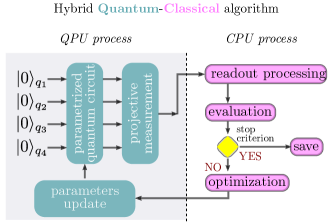
Figure 1: Hybrid quantum-classical algorithm for data-driven quantum circuit learning (DDQCL). Sketch for a simple case of four qubit setup, in which, the probability distribution of the resulting quantum state is used as the generative model for the ML task. Training of the quantum circuit towards the generation of such quantum model is achieved by a continuous update of the quantum circuit parameters by a classical optimizer. The quantum model distribution is obtained from simple projective measurements in the computational basis, which, after readout processing, it is compared with the target distribution dictated by the data set. The optimizer updates the quantum circuit parameters until a stop criterion is met, e.g., a maximum number of iterations or a desired value of the optimization cost function is reached.

Experimental implementations of DDQCL where the entire learning process performed on-hardware have been recently demonstrated in both, superconducting qubits Hamilton et al. (2018) and ion-trap quantum computers Zhu et al. (2018). In the superconducting qubits implementation emphasis was given to the exploration of different circuit ansätze, while in the ion-trap experiments, in addition to consideration of different proposals for the quantum processing unit (QPU) side of the pipeline, emphasis was given as well to the importance of the optimizer used.

Each of the independent training curves of DDQCL and any HQC algorithm requires several iterations which correspond to the updates of the PQC. This procedure, in turn, represents typically thousands of circuits that need to be executed in hardware, per training curve. As seen in any of the aforementioned experimental implementation of DDQCL on-hardware, usually only one learning curve is performed, for each of the components to be optimized, e.g., circuit ansatz or optimizer. As shown in this work and elsewhere Benedetti et al. (2018), for most of the optimizers previously considered in the literature, the variance from the solver’s random initialization is one of the most significant sources of uncertainty when reporting the performance of the HQC algorithm. Thus, one successful run does not necessarily correlates with the typical performance of the solver; none of the studies to date seem to afford multiple runs per each of the settings studied. To assess the impact of any choice within the HQC algorithm and to draw robust conclusions about the impact of several entangling connectivities or the performance of any optimizer against another, several runs per setting need to be performed.

In this work we present the first experimentally robust comparison of each of the aspects of HQC algorithms, using DDQCL as the working framework since it provides figure merit for the performance of each of the knobs explored. To achieve this systematic and robust study, we leverage on Rigetti’s Quantum Cloud Services (QCS™) and its enhanced framework for handling the requirements of HQC algorithms efficiently. Some unique features of this platform include pre-compilation of the PQC programming cycles, active reset allowing for faster repetition rates, and low-latency due to co-location of the quantum and classical hosts.

II DDQCL execution on Rigetti’s QPU

As in previous on-hardware implementations of DDQCL Hamilton et al. (2018); Zhu et al. (2018), for the machine learning task we consider a small artificial classical dataset, Bars and Stripes (BAS), which consists of patterns of $n\times m$ binary images of bars or stripes, and denoted here as $(n,m)$BAS. As shown in Fig. 2, the $(2,2)$BAS dataset contains six different binary images. We encode the binary imagines into bitstrings, associating dark pixels to “1” and white pixels to “0”, i.e. $\blacksquare=1$ and $\Box=0$. In Figure 2, we present the patterns for $(2,2)$BAS and the label convention to use for binary image encoding. Following that convention the $(2,2)$BAS dataset contains $\{0000,1010,0101,0011,1100,1111\}$ that leads to a simple distribution $P_{\cal X}(\bm{x})=1/6$ for $\bm{x}\in$ $(2,2)$BAS. The goal for the circuit learning approach is to prepare a state $|\psi\rangle=\sum_{\bm{x}\in\{0,1\}^{4}}\alpha_{\bm{x}}|\bm{x}\rangle$ with $|\alpha_{\bm{x}}|^{2}=1/6$ for $\bm{x}\in(2,2)$BAS and $|\alpha_{\bm{x}}|^{2}=0$ otherwise.

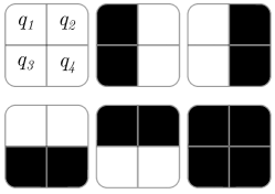
Figure 2: $(2,2)$ BAS classical data set. The patterns that belong to $(2\times 2)$ Bars and Stripes dataset are shown. In the first pattern (on the top left corner), the label convention is depicted to encode the patterns into classical bitstrings, e.g., for the second binary image (from the top left corner to the right), $(q_{1},q_{2},q_{3},q_{4})=(\blacksquare,\Box,\blacksquare,\Box)=(1,0,1,0)\rightarrow 1010$.

For the experimental implementation of DDQCL, we consider a four-qubit subunit connected in star and line entangling topology, according to the connectivity constraints in the 16-qubit Aspen™quantum computer (see insets in Fig 3). The main building blocks for the construction of the quantum circuit ansatz (see, e.g. top right in Fig. 3) relies on two observations. (i) The use of CZ entangling gates is native to the Rigetti QPU. This sets our preference towards these gates over either CNOTs or Mølmer-Sørensen gates which were used in previous DDQCL implementations Hamilton et al. (2018); Zhu et al. (2018) on either the IBM Tokyo or ion-trap quantum computer, respectively. (ii) Instead of using arbitrary single-qubit gates intersperse or alternating with two-qubits gates, we used here just $R_{y}(\theta)$ rotations. Given that all the entries of the $R_{y}(\theta)$ are real, along with the CZ gates produces quantum states with real amplitudes only. Note this is a not limitation towards the quantum model used in the generative task since it is enough to consider $\alpha_{\bm{x}}\in{\rm I\!R}$. In Appendix B.1, we provide more intuition of the layout for this circuit ansatz. This last choice of going from single-arbitrary rotations to just $R_{y}$ rotations is desirable since it reduces the number of parameter in the quantum model, therefore helping the classical optimizer in this high-dimensional search space.

The progress of this machine learning task is evaluated by the Jensen-Shannon divergence cost function (details in Appendix A), that compares the probabilistic distribution of the circuit output with the target distribution. With the learning score record, the quantum circuit parameters are updated by an optimizer running on a classical processor; this optimization in pursuit of a minimum score is the classical part of the generative model approach.

III results

For our experimental and numerical benchmarking study we used three solvers: the Zeroth-Order Optimization package (ZOOPT) Liu et al. (2017), the Stochastic Variation of Hill-Climbing type algorithm (SVHC) Perdomo et al. (2019a), and a classical stochastic gradient descent based solver (ADAM) Kingma and Ba (2014) (for configuration details, see Appendix B.2).

We consider a specific region of the QPU to run the experiments (see QPU layout inside Figure  3). For each of the settings to be explored, i.e. the choice of solver or the entangling connectivity topology or the varying depth of the circuit, we performed five independent DDQCL from random initializations of the parameters. In each DDQCL, 2000 different realizations of the PQC were evaluated, and from each of them, 3000 shots were taken as readouts in the computational basis. Before every batch of these five independent runs, we performed the characterization of the matrix to be used for readout correction and use it to post-process the experimental histograms built from every 3000 shots (see Appendix  B.3 for details). In Figure 3, we present the main results, where the best learned probabilistic model is depicted with $D_{KL}$ values 0.44 and 0.14 for line and star topology, respectively. Those values were reached using the ZOOPT optimizer. $D_{KL}$ corresponds to the Kullback-Leibler divergence and it is the gold standard when comparing the closeness between two probability distributions, with $D_{KL}=0.0$ meaning that the quantum model and the target distribution match. Estimation of $D_{KL}$ from the experimental histogram also allow us to compare to previous experimental realizations Hamilton et al. (2018); Zhu et al. (2018). From these it can be seeing that our DDQCL implementation on the Rigetti QPU ($D_{KL}=0.14$) is better than the best model obtained in the IBM Tokyo quantum processor ($D_{KL}=0.36$), and comparable to the best results obtained in the trapped-ion quantum computer ($D_{KL}=0.09$)

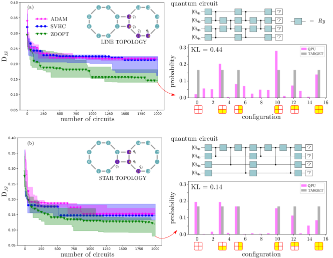
Figure 3: DDQCL on the $(2,2)$BAS and Stripes dataset, using different solvers and topologies. In the upper/lower panel (a/b) is depicted the learning progress for two layers of entangling circuits with a line/star topology connectivity using ADAM, SVHC, and ZOOPT classical optimizers. Besides, in the panels are shown the quantum circuit model and the comparison between the probability distribution corresponding to the lowest cost and the target distribution. In that comparison, it is shown the Kullback-Leibler divergence cost to get to the target distribution from the QPU best result.

In addition to testing the performance of different types of optimizers, we consider different circuits depths. For these experiments, we consider a circuit with one round of entangling gates with 3 CZ’s and 10 local rotations, and the circuit used for the optimizers comparison corresponding to two rounds of entangling gates with 16 local rotations and 6 CZ’s (see ${\cal L}_{1}$ and ${\cal L}_{2}$ in Figure 4, respectively). In star topology configuration, a significant improvement is observed with the addition of a second entangling round, while for the line topology configuration, there is significantly less improvement (or at least slower convergence) from the addition of a second entangling round. To understand this apparent faster convergence and better results from the star entangling topology compared to its line analog, we performed in-silico simulations with the same optimizers. From these simulations on noiseless qubits (see Appendix C), it is hard to advocate for a clear advantage of the star connectivity over the line entangling ansatz. Therefore, this discrepancy in results between in-silico simulations and the on-hardware ones is not to the topology itself, but most likely it is due to the quality of the qubits used for each experiment, with better quality for the subset used for the star experiments.

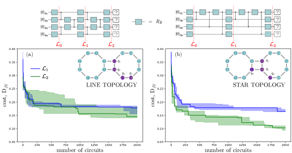
Figure 4: Learning improvement with circuit depth. In this Figure, we show the learning improvement with the circuit depth on the line and star topology. We define an entangling layer as a set of entangling gates ${\cal U}_{2}$ overall qubits according to the topology. For line topology, after simplification, a layer for 4 qubits consists of 6 rotations $R_{y}$ and 3 CZs, see the quantum circuit over panel (a). The same amount of rotations $R_{y}$ and CZ’s stands for the star topology, see the quantum circuit over panel (b). A relative improvement due to circuit depth is presented using star topology against the line topology, in which the variance of the learning curve for 1 layer overlaps the variance of the learning curve for 2 layers. In the experiments we consider qubits in similar regions of the device (see layouts inside) according to the topologies.

For completeness, in Table 1 we report the values for the qBAS score, calculated as detailed in Ref. Benedetti et al. (2018).

Table 1: Performance figures of merit from main experimental features explored in this work related to different optimizers and circuit ansätze (star versus line).

IV Summary and outlook

We performed a robust implementation and a comparison on-hardware of several components of primal importance affecting the performance of hybrid quantum-classical algorithms. The factors tested include the circuit entangling layout and its depth, the selection of the classical optimizer, and the impact of post-processing strategies such as readout correction.

Although results here show that the choice of each of these components affects the performance significantly, the study presented here is far from exhaustive. It is known that optimizing each of the classical solvers in its own is a hard task, and it would be left to future work to address this selection, for example, by using an automatic routine for hyperparameter setting (see, e.g., Snoek et al. (2012)).

Another interesting direction would be to try some recent extensions of DDQCL experimentally, proposing a gradient-based training approach Liu and Wang (2018) or by adding ancillary qubits to enhance the power of the quantum generative model Du et al. (2018).

We hope hybrid approaches on concrete data sets and real-world applications, such as the generative modeling task highlighted here, become a more significant way to benchmark and measure the power of quantum devices. The qBAS score described in Ref. Benedetti et al. (2018) and measured here for our experimental results represents a way to measure the power of these NISQ devices, beyond values reported for the fidelity of single and two-qubit gates. To move to a quantum ready stage, it is essential we move towards evaluating the capacity and performance of the device as a whole. We believe developing the infrastructure to develop robust benchmarking studies like the one presented here is an essential step towards a meaningful comparison among different algorithmic and hardware proposals.

Appendix A DDQCL pipeline

In this work we implement a hybrid quantum-classical algorithm for unsupervised machine learning tasks introduced in Benedetti et al. (2018) at Rigetti’s superconducting quantum computer (QPU). In the following we present a short introduction of the approach, for a complete discussion see Benedetti et al. (2018). The algorithm generates a probability distribution model for a given classical dataset ${\cal X}=\{\bm{x}^{(1)},\bm{x}^{(2)},\cdots,\bm{x}^{(D)}\}$ with distribution $P_{\cal X}$. Without lost of generality, the elements of ${\cal X}$ can be considered as $N$-dimensional binary vectors $\bm{x}^{(i)}\in\{0,1\}^{N}$ for $i=1,....,D$, allowing a direct connection with the basis of an $N$-qubit quantum state, i.e., $\bm{x}^{(i)}\rightarrow|\bm{x}^{(i)}\rangle=|x_{1}^{(i)},...,x_{N}^{(i)}\rangle$ for $i=1,...,D$. The goal is to prepare a quantum state $|\psi\rangle=\sum_{\bm{x}\in\{0,1\}^{N}}\alpha_{\bm{x}}\,|\bm{x}\rangle$, with a probability distribution that mimics the dataset distribution, $|\langle\bm{x}|\psi\rangle|^{2}=|\alpha_{\bm{x}}|^{2}=P_{\cal X}(\bm{x})$ for $\bm{x}\in\{0,1\}^{N}$.

The required quantum state $|\psi\rangle$ is prepared by tuning a PQC composed of single rotations and entangling gates with fixed depth and gate layout. In general, the circuit parameters of amount $L$ can be written in a vector form ${\bm{\theta}}=\{\theta_{1},...,\theta_{L}\}$, that prepares a state $|\psi_{\bm{\theta}}\rangle$ with distribution $P_{\bm{\theta}}$. The algorithm varies $\bm{\theta}$ to get a minimal loss from $P_{\bm{\theta}}$ to $P_{\cal X}$. Here, we consider the Jensen-Shannon divergence ($D_{\rm JS}$) to measure the loss, and determine how to update $\bm{\theta}$ using a classical optimizer.

The $D_{\rm JS}$ divergence is a symmetrized and smoothed version of the Kullback-Leibler divergence ($D_{\rm KL}$), defined as

$$D_{\rm JS}(P|Q)=\frac{1}{2}D_{\rm KL}(P|M)+\frac{1}{2}D_{\rm KL}(Q|M),$$ (1)

where $P$ and $Q$ are distributions, and $M=(P+Q)/2$ their average. The Kullback-Leibler divergence is defined as

$$D_{\rm KL}(X|M)=\sum_{s\ \in\ \{0,1\}^{N}}X(s)\,{\rm ln}\left(X(s)\right)-\sum_{s\ \in\ \{0,1\}^{N}}X(s)\,{\rm ln}\left(M(s)\right),$$ (2)

for $X\in\{P,Q\}$.

After the algorithm evaluates the cost from $P_{\bm{\theta}}$ to $P_{\cal X}$, it follows a quantum circuit parameters update in pursuit to a minimal cost. This procedure is done by an optimizer that runs on a classical processor unit (CPU). In summary, the algorithm chooses a random set of parameters $\bm{\theta}$, evaluates the cost from $P_{\bm{\theta}}$ to the target $P_{\cal X}$ through the Jensen-Shannon divergence $D_{\rm JS}(P_{\bm{\theta}}|P_{\cal X})$, and updates $\bm{\theta}$ minimizing the cost. This procedure is repeated several times (iterations) until a convergence criterium is met, for instance, a maximum number of iterations.

Appendix B Experimental details

B.1 Quantum circuit model design

Since the quantum state probabilistic distribution does not depend on local quantum state phases, we chose a layout of the model circuit that prepares real amplitude quantum states. We consider the following two-qubit ansatz as the base to design $N$-qubit the circuit layout for DDQCL,

$${\cal U}_{2}(\theta,\gamma,\beta)|00\rangle = R_{1}^{\beta}\,R_{0}^{\gamma}\,{\rm CZ}_{01}\,R_{0}^{\theta}\,|00\rangle$$ (3)

$$= \sum_{s\in\{0,1\}^{2}}\!\!\!\alpha_{s}|s\rangle$$

therein $R_{k}^{\theta}=\exp[-i\,\theta\,\sigma^{y}_{k}/2]$ is a local rotation around $y$-axis in the Bloch sphere on the $k$th qubit and ${\rm CZ}_{kl}$ the control phase shift gate between $k$th and $l$th qubits. The gate ${\cal U}_{2}$ defines a one-to-one map $[0,2\pi)^{3}\leftrightarrow S^{3}$, that ensures the preparation of any 2 qubit state with real probability amplitudes Perdomo et al. (2019b), i.e. $\alpha_{s}\in{\rm I\!R}$ for $s\in\{0,1\}^{2}$. For setups with more than 2 qubits, we use ${\cal U}_{2}$ to entangle different pairs of qubits depending on their connectivity, until getting a fully controlled entangled state. In this study, we consider four qubits with different connections (topologies) according to the Rigetti’s quantum computer architecture. We designed several circuits for line and star topologies using up to $L=16$ local rotations and 6 CZ’s (see Figure 3).

In-silico simulations on noiseless qubits show that this circuit layout can learn a quantum model capable of successfully reproducing the target probability from the $(2,2)$BAS (see Appendix C).

As pointed in the main text, one of the advantages of this circuit layout compared to the one considering arbitrary single-qubit rotations is the reduction in the number of parameters. On the other hand, it is important to note that having the additional parameters could in principle help the search since these open more paths in the Hilbert space, resulting in an increased number of states that could lead to a perfect $P_{\cal X}$ (see e.g., the discussion in the “Entanglement entropy of BAS(2,2)” section in the Supp. Material of Ref. Benedetti et al. (2018)). This trade-off between flexibility in the quantum model and difficulty in optimization is beyond the scope of this work, and it would be an interesting research direction to explore.

B.2 Classical optimizers

For our experimental and numerical benchmarking study we used three solvers: the Zeroth-Order Optimization package (ZOOPT) Liu et al. (2017), the Stochastic Variation of Hill-Climbing type algorithm (SVHC) Perdomo et al. (2019a), and a classical stochastic gradient descent based solver (ADAM) Kingma and Ba (2014). For the case of ZOOPT and SVHC, we handle the stochastic nature of the cost function via the ”value suppression” setting. Additionally, a set of $N_{\rm ini}=3L$ randomly chosen initial circuits are evaluated to get a searching starting point. For ADAM, we consider the setup used in Ref. Hamilton et al. (2018), with learning rate $\alpha=0.2$, decay rates $\beta_{1}=0.9$, and $\beta_{2}=0.999$.

B.3 Improvement via readout correction

DDQCL is based on the probability distribution of the $N$ qubit quantum state, which is in turn transformed into resulting bitstrings $\{0,1\}^{N}$, denoted as shots in the main text. Unfortuantely, no device is 100% free of errors in this transformation from quantum state to bitstring output. Next we describe a simple model to cope with this classical readout channel. Although there have been other procedures which are scalable Kandala et al. (2017); Dumitrescu et al. (2018); Magnard et al. (2018), here we exploit our small number of qubits to make the least number of assumptions on the channel and perform an exponential number of experiments, which need to be done once to characterize the channel.

The simple error readout correction implemented here consist of the measurement characterization of all the $2^{N}$ projectors $\Pi_{x}=|x\rangle\langle x|$, with $x\in\{0,1\}^{4}$ for the (2,2)BAS realization here. Suppose you trivially prepare any of the $2^{4}$ states of the computational basis, e.g., $x=0010$. In a noiseless scenario that measurement should yield a bitstring $x=0010$ in the classical register for every single shot, allowing the computation of the $P_{x}=1.0$, as expected from preparation. However, in the experiment the readouts correspond to different elements $y\in\{0,1\}^{4}$ with a distribution $p(y|x)$ due to assignment errors. In our procedure, we use a large number of readouts (set to 10000 shots) to compute the distribution $p(y|x)$, after trivial preparation of each $x\in\{0,1\}^{4}$ . Each of the $p(y|x)$ is used as the $x$-th column of the transition matrix $M$. Thus, any quantum state with population $P_{x}$ is related with actual observed output distribution $P_{y}$ as $P_{y}=MP_{x}$. To recover the original distribution from the quantum state, we invert the relation between $P_{x}$ and $P_{y}$, i.e. $P_{x}=M^{-1}P_{y}$. Before each batch of five of learning curves, we calculate the inverse transformation $M^{-1}$ and apply this to the readout distribution; this defines a post-measurement process before the score and optimization steps.

To test the efficacy of this procedure, in Figure 5, we present the training with the bare and the readout corrected training. The latter shows significant improvement with a minimal score of KL $\sim 0.13$ from $\sim 1.0$ obtained using bare readouts. Therefore, we adopted the readout correction for all the experiments reported in the main text.

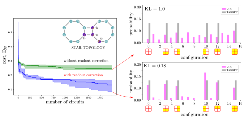
Figure 5: Comparison of DDQCL with and without readout correction. Full learning curve is shown (left) with and without readout correction (blue and green line, respectively). Without error correction, the minimal value reached for the KL divergence is $\sim 1.0$, which is closer to a random distribution, and far from the target one (see histograms on the upper right). On the other hand, the training curve with readout correction reached a value of $KL\sim 0.13$, which is a significant improvement in the DDQCL.

Appendix C In-silico simulations

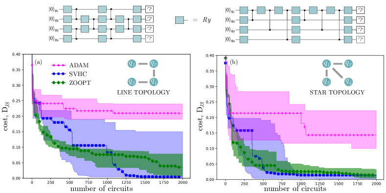
Figure 6: DDQCL simulations in-silico, and under the assumption of noiseless qubits, but taking into account the stochasticity from finite readouts. In this simulations we used 3000 shots per circuit.

Table 2: Performance figures of merit from in-silico simulations of the different HQC features explored in this work.