Compact Feature-Aware Hermite-Style
High-Order Surface Reconstruction

Abstract

High-order surface reconstruction is an important technique for CAD-free, mesh-based geometric and physical modeling, and for high-order numerical methods for solving partial differential equations (PDEs) in engineering applications. In this paper, we introduce a novel method for accurate and robust reconstructions of piecewise smooth surfaces from a triangulated surface. Our proposed method extends the Continuous Moving Frames (CMF) and the Weighted Averaging of Local Fittings (WALF) methods (Engrg. Comput. 28 (2012)) in two main aspects. First, it utilizes a Hermite-style least squares approximation to achieve fourth and higher-order accuracy with compact support, even if the input mesh is relatively coarse. Second, it introduces an iterative feature-aware parameterization to ensure high-order accurate, $G^{0}$ continuous reconstructions near sharp features. We present the theoretical framework of the method and compare it against CMF and WALF in terms of accuracy and stability. We also demonstrate that the use of the Hermite-style reconstruction in the solutions of PDEs using finite element methods (FEM), and show that quartic and sextic FEMs using the high-order reconstructed surfaces produce nearly identical results as using exact geometry while providing additional flexibility.
Keywords: high-order methods; surface reconstruction; weighted least squares; Hermite approximations; geometric discontinuities; finite element methods

1 Introduction

Surface meshes and their manipulations are critical for geometric modeling, meshing, numerical simulations, and other related problems. Some example problems that involve manipulating surface meshes include mesh generation and mesh enhancement for high-order finite element methods [5], mesh smoothing in ALE methods [1], mesh adaptation in moving boundary problems [11], and geometric modeling and meshing in computer graphics [4, 20]. In these settings, it is often critical to have a high-order accurate representation of the surface to support the mesh manipulations. The high-order surfaces are also important for modern numerical discretization methods, such as quadratic, quartic, and even sextic finite element methods and higher-order spectral element methods, which have become increasingly in recent years. However, a continuous CAD model is often not available. Instead, only a surface mesh, typically with piecewise linear or bilinear faces, is available.

In this paper, we consider the problem of reconstructing a high-order accurate, continuous surface from a surface triangulation. We refer to this problem as high-order surface reconstruction (or simply high-order reconstruction). By “high order,” we mean that the method should be able to deliver more than second-order accuracy, and preferably fourth or higher order, compared to just first or second order accuracy of traditional techniques. The high-order accuracy is important for accurate treatment of boundary conditions along curved boundaries, especially with high-order finite element methods.

In [12], four requirements were posed for high-order reconstruction:

Geometric accuracy:

The reconstruction should be accurate and asymptotically convergent to the exact surface to high order under mesh refinement.

Continuity:

The reconstructed surface should be continuous to some degree (e.g., $G^{0}$, $G^{1}$, or $G^{2}$ continuous, depending on applications).

Feature preservation:

The reconstruction should preserve sharp features (such as ridges and corners) in the geometry.

Numerical stability:

The reconstruction should be numerically stable and must not be oscillatory under noise.

Different applications may have different emphases on the requirements. For example, in computer graphics and geometric design, the visual effect may be the ultimate goal, so smoothness and feature preservation may be more important. Our focus in this paper is on numerical solutions of partial differential equations (PDEs), for which the numerical accuracy and stability are critical. Indeed, if the geometry is low-order accurate, the numerical solutions of a high-order finite element method will most likely be limited to low-order accuracy. An unstable surface approximation with excessive oscillations can have even more devastating effect on the numerical simulations. Some efforts, such as isogeometric analysis [9], aim to improve accuracy by using continuous CAD models directly in numerical simulations, but CAD models are often not available, such as in moving boundary problems, or they may be impractical to be used directly, such as on large-scale supercomputers. When only a mesh is given, a high-order reconstruction may sometimes be the best option, in that they provide additional flexibility and can deliver the same accuracy as using exact geometry.

Two methods, called Continuous Moving Frames (CMF) and Weighted Averaging of Local Fittings (WALF), were proposed in [12], for reconstructing a piecewise smooth surfaces. Both methods were based on weighted least squares (WSL) approximations using local polynomial fittings with the assumption that the vertices of the mesh accurately sample the surface, and the connectivity of the mesh correctly represent the topology of the surface. These methods can achieve fourth- and even higher order accuracy, and WALF guarantees $G^{0}$ continuity for smooth surfaces. In contrast, most other methods could achieve only first- or second-order accuracy. Between CMF and WALF, the former tends to be more accurate whereas the latter tends to be more efficient. However, both CMF and WALF had two key limitations. First, if the input mesh is relatively coarse, then there may be a lack of points in the stencil, so the methods are forced to use low-order approximations to avoid instability [12]. This loss of accuracy tends to happy more pronounced near boundaries or sharp features (i.e., ridges and corners), where the stencils tend to be one-sided. Second, $G^{0}$ continuity may be lost near sharp features, so the reconstructed surface may not be “watertight.” As a result, when used to generate high-order finite element meshes, the parameterization of the surface elements incident on sharp features may suffer from a loss of smoothness and in turn loss of precision in the numerical solutions.

In this paper, we address these limitations of CMF and WALF to achieve high-order accuracy and $G^{0}$ continuity near sharp features. To this end, we extend these methods in two main aspects. First, we introduce a Hermite-style weighted least squares approximation, to take into account both point locations as well as normals in surface reconstruction. We assume that the point coordinates and normals are high-order accurate, which, for example, may be obtained from the original CAD models or obtained from solutions of differential equations. A key advantage of this Hermite-style reconstruction is that it allows much more compact stencils, so high-order accuracy can be achieved even with relatively coarse input meshes. Second, we introduce an iterative feature-aware parameterization for constructing high-order surface elements, so that these surface elements can define a $G^{0}$ continuous surface with smooth parameterizations and uniform high-order accuracy.

Using both point and normal for numerical approximation on discrete surfaces is not a new idea. It is analogous to Hermite interpolation in numerical analysis. For surface modeling, Walton [20] defined an approach to reconstruct $G^{1}$ continuous surfaces. Another example is the curved PN-triangles [19]. Other related work includes [7], in which points and normals are used together for estimating curvatures. However, to the best of our knowledge, our proposed technique is among the first that leverage both points and normals to deliver guaranteed high-order accuracy in surface reconstructions with sharp features. As a result, it provides a valuable alternative to the traditional CAD models, such as NURBS [3] and T-splines [17] for engineering applications. In particular, it provides a flexible approach for high-order methods for solving PDEs, for which we will demonstrate that high-order reconstructed surfaces enable nearly identical PDE solutions as using exact geometry during mesh generation.

Besides the Hermite-style reconstruction, another contribution of this work is to identify the significance of the smoothness of parameterizations near features. Traditionally, smoothness in surface reconstruction had focused on high-order (e.g., $G^{1}$, $G^{2}$, and even $G^{\infty}$) continuity. For example, the reconstruction in [20] aimed for $G^{1}$ continuity, and the moving least squares (MLS) [15, 4] aimed for $G^{\infty}$ continuity. However, such high-order continuity does not have direct correlation with the accuracy of the reconstructed surface or numerical PDEs. In particular, the $G^{1}$ reconstruction of Walton [20] is no more accurate than the piecewise linear surface [12]. The MLS reconstruction was conjectured in [15], but in practice it is non-convergent even for simple geometries such as a torus [12]. These higher-order continuities introduce additional difficulties in resolving sharp features. In contrast, our method aims for only $G^{0}$ continuity, but we emphasize the smoothness of the parameterization of high-order surface elements near sharp features, and we show that it has a direct correlation with the accuracy of the high-order surface reconstruction and the numerical solutions of FEM.

The remainder of the paper is organized as follows. Section 2 presents some background knowledge, including local polynomial fittings and the method of weighted least squares. Sections 3 and 4 introduce the algorithms of Hermite-style weighted least squares for high-order surface and curve reconstructions, respectively. Section 5 describes the construction of a $G^{0}$ continuous surface using high-order parametric elements with an iterative feature-aware parameterization. Section 6 assesses the proposed method in terms of geometric accuracy and feature preservation, compares it against CMF and WALF, and demonstrates its effectiveness as an alternative of exact geometry in PDE discretizations. Section 7 concludes the paper with some discussions on the future work.

2 Background

In this section, we review some basic concepts related to surfaces and space curves, followed by a brief review of weighted least squares (WLS) approximations and WLS-based surface reconstructions using CMF and WALF. These techniques are the foundations of the feature-aware Hermite-style reconstruction proposed in this paper.

2.1 Surfaces and Space Curves

2.1.1 Smooth Surfaces.

Consider a smooth surface $\Gamma$ defined in the global $xyz$ coordinate system. Given a point $\boldsymbol{x_{0}}=[x_{0},y_{0},z_{0}]^{T}$ on the surface (note that for convenience we treat points as column vectors), let the origin of the local frame be at $\boldsymbol{x}_{0}$. Let $\boldsymbol{m}_{0}$ be an approximate normal vector with unit length at $\boldsymbol{x_{0}}$. Let $\boldsymbol{s}_{0}$ and $\boldsymbol{t}_{0}$ denote a pair of orthonormal basis vectors perpendicular to $\boldsymbol{m}_{0}$. The vectors $\boldsymbol{s}_{0}$, $\boldsymbol{t}_{0}$, and $\boldsymbol{m}_{0}$ form the axes of a local $uvw$ coordinate system at $\boldsymbol{x}_{0}$. Let $\boldsymbol{Q}_{0}$ be the matrix composed of column vectors $\boldsymbol{s}_{0}$, $\boldsymbol{t}_{0}$, and $\boldsymbol{m}_{0}$, i.e., $\boldsymbol{Q}_{0}=\left[\boldsymbol{s}_{0},\,\boldsymbol{t}_{0},\,\boldsymbol{m}_{0}\right]$. Any point $\boldsymbol{x}$ in the global coordinate system can be then transformed to the point

$$\boldsymbol{p}(\boldsymbol{u})=\left[u,v,w(\boldsymbol{u})\right]^{T}=\boldsymbol{Q}_{0}^{T}(\boldsymbol{x}-\boldsymbol{x}_{0})$$ (1)

in the local frame, where $\boldsymbol{u}=\left[u,v\right]^{T}$. Since $\boldsymbol{m}_{0}$ is an approximate normal vector, $w(\boldsymbol{u})$ is expected to be one-to-one in a neighborhood of $\boldsymbol{x}_{0}$. We refer to $f(\boldsymbol{u})=w(\boldsymbol{u})$ as the local height function about $\boldsymbol{x}_{0}$. This transformation is important for high-order surface reconstruction, since it allows reducing the problem to high-order approximations to the local height function. The vectors $\boldsymbol{p}_{u}$ and $\boldsymbol{p}_{v}$ are tangent to the surface in the local frame. Let $\ell=\left\|\boldsymbol{p}_{u}\times\boldsymbol{p}_{v}\right\|=\sqrt{1+\left\|\boldsymbol{\nabla}f\right\|^{2}}$, which is the area measure. The unit normal to the surface in the local frame is then given by

$$\hat{\boldsymbol{n}}=\frac{\boldsymbol{p}_{u}\times\boldsymbol{p}_{v}}{\ell}=\frac{1}{\ell}\left[\begin{array}[]{c}-\boldsymbol{\nabla}f\\ 1\end{array}\right].$$ (2)

This connection between the normal $\hat{\boldsymbol{n}}$ and the gradient of local height functions will be important for Hermite-style surface reconstruction.

2.1.2 Space Curves.

For piecewise smooth surfaces, there can be ridge curves (or feature curves). These curves are space curves, in that they are embedded in $\mathbb{R}^{3}$ and they may not be coplanar. Similarly, for an open surface, its boundary curve is a space curve, and it can be treated in the same fashion as feature curves.

Given a point $\boldsymbol{x}_{0}$ on a space curve $\gamma$ in $\mathbb{R}^{3}$, let $\boldsymbol{s}_{0}$ be an approximate tangent vector of unit length. Let $\boldsymbol{m}_{0}$ and $\boldsymbol{b}_{0}$ denote a pair of orthonormal basis functions perpendicular to $\boldsymbol{s}_{0}$. The vectors $\boldsymbol{s}_{0}$, $\boldsymbol{m}_{0}$, and $\boldsymbol{b}_{0}$ form the axes of a local $uvw$ coordinate system at $\boldsymbol{x}_{0}$. Let $\boldsymbol{Q}_{0}=\left[\boldsymbol{s}_{0},\,\boldsymbol{m}_{0},\,\boldsymbol{b}_{0}\right]$. Then, any point $\boldsymbol{x}$ in the global coordinate system can be transformed to

$$\boldsymbol{p}(u)=\left[u,v(u),w(u)\right]^{T}=\boldsymbol{Q}_{0}^{T}(\boldsymbol{x}-\boldsymbol{x}_{0})$$ (3)

in the local frame. We refer to $\boldsymbol{f}(u)=[v(u),w(u)]^{T}$ as a vector-valued local height function, of which each component is one-to-one in a neighborhood of $\boldsymbol{x}_{0}$. The length measure is $\ell=\|\boldsymbol{p}(u)\|=\sqrt{1+\left\|\boldsymbol{f}^{\prime}(u)\right\|^{2}}$. The unit tangent to the curve in the local frame is then

$$\hat{\boldsymbol{t}}=\frac{\boldsymbol{p}}{\ell}=\frac{1}{\ell}\left[\begin{array}[]{c}1\\ \boldsymbol{f}^{\prime}(u)\end{array}\right],$$ (4)

which will be important for Hermite-style curve reconstruction.

2.2 Local Weighted Least Squares Fittings.

Weighted least squares is a powerful method for constructing high-order polynomial fitting of a smooth function. Let us first derive it for a function $f(\boldsymbol{u}):\mathbb{R}^{2}\rightarrow\mathbb{R}$ at a given point $\boldsymbol{u}_{0}=\left[0,0\right]^{T}$, where $f$ is the local height function in surface reconstruction. Suppose $f$ is smooth and its value is known only at a sample of $m$ points $\boldsymbol{u}_{i}$ near $\boldsymbol{u}_{0}$, where $1\leq i\leq m$. We refer to these points as the stencil for the fitting. The 2D Taylor series of $f(\boldsymbol{u})$ about $\boldsymbol{u}_{0}$ is given by

$$f(\boldsymbol{u})=\sum_{q=0}^{\infty}\sum_{j,k\geq 0}^{j+k=q}c_{jk}u^{j}v^{k},$$ (5)

where $c_{jk}=\dfrac{1}{j!k!}\dfrac{\partial^{j+k}}{\partial u^{j}\partial v^{k}}f(\boldsymbol{0})$. Suppose $f$ is continuously differentiable to $(p+1)$st order for some $p>1$. $f(\boldsymbol{u})$ can be approximated to ($p+1$)st order accuracy about $\boldsymbol{u}_{0}$ as

$$f(\boldsymbol{u})=\sum_{q=0}^{p}\sum_{j,k\geq 0}^{j+k=q}c_{jk}u^{j}v^{k}+\mathcal{O}\left(\|\boldsymbol{u}\|^{p+1}\right).$$ (6)

The first term in (6) is the degree-$p$ Taylor polynomial about the origin, which has $n=(p+1)(p+2)/2$ coefficients, namely $c_{jk}$ with $0\leq j+k\leq p$. Assume $m\geq n$, and let $f_{i}$ denote $f(\boldsymbol{u}_{i})$. We then obtain a system of $m$ equations

$$\sum_{q=0}^{p}\sum_{j,k\geq 0}^{j+k=q}c_{jk}u_{i}^{j}v_{i}^{k}\approx f_{i}$$ (7)

for $1\leq i\leq m$. The equation can be written in matrix form as $\boldsymbol{A}\boldsymbol{x}\approx\boldsymbol{b}$, where $\boldsymbol{A}$ is a generalized Vandermonde matrix, $\boldsymbol{x}$ is composed of $c_{jk}$, and $\boldsymbol{b}$ is composed of $f_{i}$.

The generalized Vandermonde system obtained from (7) is rectangular. In general, it can be solved by posing as a minimization of the weighted norm of the residual vector $\boldsymbol{r}=\boldsymbol{b}-\boldsymbol{A}\boldsymbol{x}$, i.e.,

$$\min_{\boldsymbol{x}}\|\boldsymbol{r}\|_{\boldsymbol{W}}\equiv\min_{\boldsymbol{x}}\|\boldsymbol{W}(\boldsymbol{A}\boldsymbol{x}-\boldsymbol{b})\|_{2},$$ (8)

where $\boldsymbol{W}=\mbox{diag}\{\omega_{1},\omega_{2},\dots,\omega_{m}\}$ is diagonal and is referred to as the weighting matrix. The weights in $\boldsymbol{W}$ assign priorities to different rows in the generalized Vandermonde system, where each row corresponds to a different point in the stencil. If both $\boldsymbol{A}$ and $\boldsymbol{W}$ are nonsingular matrices, then $\boldsymbol{W}$ has no effect on the solution. However, if $m\neq n$ or $\boldsymbol{A}$ is singular, then different $\boldsymbol{W}$ would lead to different solutions. Let $\boldsymbol{T}\in\mathbb{R}^{n\times n}$ be a scaling matrix, and we arrive at the least squares problem

$$\boldsymbol{W}\boldsymbol{A}\boldsymbol{T}\boldsymbol{y}\approx\boldsymbol{W}\boldsymbol{b},$$ (9)

and then $\boldsymbol{x}=\boldsymbol{T}\boldsymbol{y}$. In general, given a weighting matrix $\boldsymbol{W}$, let $\boldsymbol{v}_{i}$ denote the $i$th column vector of $\boldsymbol{W}\boldsymbol{A}$. We choose

$$\boldsymbol{T}=\text{diag}\{1/\|\boldsymbol{v}_{1}\|_{2},\dots,1/\|\boldsymbol{v}_{n}\|_{2}\},$$ (10)

which approximately minimizes the condition number; see [8, p. 265] and [18]. We refer to this as algebraic column scaling. Alternatively, let $h$ be a length measure of the stencil, and one can scale the coordinates of $u_{i}$ and $v_{i}$ by dividing them by $h$. We refer to this as geometric scaling, which is equivalent to the algebraic scaling with $\boldsymbol{T}$ equal to the diagonal matrix composed of $h^{-j-k}$, where $j$ and $k$ are the corresponding indices of $c_{jk}$ in (7).

The matrix $\boldsymbol{W}\boldsymbol{A}\boldsymbol{T}$ may still be ill-conditioned even after scaling. For efficiency and robustness, (9) can be solved using a truncated QR factorization with column pivoting (QRCP). Specifically, let $\tilde{\boldsymbol{A}}=\boldsymbol{W}\boldsymbol{A}\boldsymbol{T}$. The QRCP is

$$\tilde{\boldsymbol{A}}\boldsymbol{P}=\boldsymbol{Q}\boldsymbol{R},$$ (11)

where $\boldsymbol{Q}$ is $m\times n$ with orthonormal column vectors, $\boldsymbol{R}$ is an $n\times n$ upper-triangular matrix, $\boldsymbol{P}$ is a permutation matrix, and the diagonal entries in $\boldsymbol{R}$ are in descending order [8]. For ill-conditioned systems, the condition number of $\boldsymbol{R}$ can be estimated incrementally; if a column results in a large condition number, its corresponding monomial should be truncated, so do the other monomials that contain it as a factor. Let $\tilde{\boldsymbol{Q}}$ and $\tilde{\boldsymbol{R}}$ denote the truncated matrices. The final solution of $\boldsymbol{x}$ is then given by

$$\boldsymbol{x}=\boldsymbol{T}\boldsymbol{P}\tilde{\boldsymbol{R}}^{-1}\tilde{\boldsymbol{Q}}^{T}\boldsymbol{W}\boldsymbol{b},$$ (12)

where $\tilde{\boldsymbol{R}}^{-1}$ denotes a back substitution step.

The solution vector $\boldsymbol{x}$ contains the coefficients $c_{ij}$, from which we obtain a polynomial $\tilde{f}(\boldsymbol{u})=\sum_{q=0}^{p}\sum_{j,k\geq 0}^{j+k=q}c_{jk}u^{j}v^{k}$. We refer to this approach for estimating the Taylor polynomial as local WLS fitting. Note that if $\boldsymbol{u}_{0}$ is a point in the stencil, we can force $\tilde{f}$ to be interpolatory at $\boldsymbol{u}_{0}$, i.e., $\tilde{f}(\boldsymbol{u}_{0})=f(\boldsymbol{u}_{0})$, by setting $c_{00}=0$ and removing the equation corresponding to $\boldsymbol{u}_{0}$. This reduces the problem to an $(m-1)\times(n-1)$ linear system, and it tends to be more accurate if the function $f$ is known to be accurate at $\boldsymbol{u}_{0}$.

2.3 Local Fittings on Triangulated Surfaces.

The local WLS fittings can be used in local high-order reconstructions of a triangulated surface, on which a feature curve is composed of a collection of edges. This requires three key components: 1) construct a local frame, 2) select a proper stencil about the vertex, and 3) define the weighting scheme.

To define the local frame at a point $\boldsymbol{x}_{0}$ on a surface, we need an approximate surface normal $\boldsymbol{m}_{0}$ at the point, which can be obtained by averaging the normals to its adjacent faces. Such an averaging is in general first-order accurate, which suffices for this purpose. Similarly, for a curve, we need an approximate tangent vector $\boldsymbol{s}_{0}$ at a point, which can be obtained by averaging the tangents to its adjacent edges.

For the stencil selection, it is simple and efficient to use mesh connectivity. For curves, as long as the points are distinct, it suffices to make the number of points to be equal to the number of coefficients, but $m>n$ may lead to better error cancellation for even-degree polynomials with nearly symmetric stencils. For a triangular mesh, we define $\mathit{k}$-ring neighborhoods, with half-ring increments, as follows:

• The 1-ring neighbor faces of a vertex $v$ are the faces incident on $v$, and the 1-ring neighbor vertices are the vertices of these faces.

• The 1.5-ring neighbor faces are the faces that share an edge with a 1-ring neighbor face, and the 1.5-ring neighbor vertices are the vertices of these faces.

• For an integer $k\geq 1$, the $(k+1)$-ring neighborhood of a vertex is the union of the 1-ring neighbors of its $k$-ring neighbor vertices, and the $(k+1.5)$-ring neighborhood is the union of the $1.5$-ring neighbors of the $k$-ring neighbor vertices.

Figure 1 illustrates this definition up to 2.5 rings. In general, for degree-$p$ fitting, we use the $(p+1)/2$-ring for accurate input. For a curve, the $\mathit{k}$-ring neighborhood can be defined similarly for an integer $k$, and we use $\left\lceil(p+1)/2\right\rceil$-ring for degree-$p$ fitting. We adaptively enlarge the ring size if there are too few points or the input is relatively noisy. This approach is efficient since it takes constant-time per vertex with a proper data structure, such as the half-facet (or the half-edge) data structure [2]. However, if the mesh is poor shared, the stencil may be highly skewed, which can be mitigated with a proper weighting scheme.

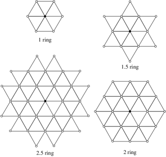
Figure 1: Illustration of $k$-ring and $k.5$-ring neighborhoods for stencil selections.

There are many options to define the weighting matrix $\boldsymbol{W}$ in (8). A commonly used weighting scheme is the so-called inverse distance weighting and its variants. The standard inverse-distance weighting assigns $\omega_{i}=1/\|\boldsymbol{x}_{i}-\boldsymbol{x}_{0}\|^{q}$ to some $q$th power. This weighting scheme assigns smaller weights for points that are farther away from the origin. However, the inverse distance has a singularity if $\boldsymbol{x}_{i}$ is too close to $\boldsymbol{x}_{0}$. This singularity can be resolved by safeguarding the denominator with some small $\epsilon$. For coarse meshes or surfaces with sharp features, it is desirable to use a small and even zero weight for $\boldsymbol{x}_{i}$ if its (approximate) normal $\boldsymbol{m}_{i}$ deviates too much from $\boldsymbol{m}_{0}$. Let $\theta_{i}^{+}\equiv\textrm{max}(0,\boldsymbol{m}_{i}^{T}\boldsymbol{m}_{0})$. We then arrive at the weight

$$\omega_{i}=\theta_{i}^{+}\left/\left(\sqrt{\|\boldsymbol{u}_{i}-\boldsymbol{u}_{0}\|^{2}+\epsilon}\right)^{q}\right.,$$ (13)

where $q=p/2$ and $\epsilon=0.1$ in [13]. The factor $\theta_{i}^{+}$ serves as a safeguard for discontinuous surface or very coarse meshes. Similarly, given a piecewise linear curve, let $\theta_{i}^{+}\equiv\textrm{max}(0,\boldsymbol{s}_{i}^{T}\boldsymbol{s}_{0})$, where $\boldsymbol{s}_{i}$ denote the approximate unit tangent at $\boldsymbol{x}_{i}$, and the same weighting scheme applies.

The inverse-distance-weighting scheme tends to give much higher weights to points closest to $\boldsymbol{x}_{0}$, especially if $\epsilon$ is close to zero. If $\boldsymbol{x}_{0}$ is not at a vertex, the vertices closest to $\boldsymbol{x}_{0}$ tend to be highly asymmetric about $\boldsymbol{x}_{0}$. In this case, it is desirable to use a weighting scheme that is flatter about the origin while being smooth and compact. A class of such functions is due to Wendland [21]. We shall consider three of these functions:

$$\psi_{3,1}(r) =(1-r)_{+}^{4}(4r+1),$$ (14)

$$\psi_{4,2}(r) =(1-r)_{+}^{6}(35r^{2}+18r+3),$$ (15)

$$\psi_{5,3}(r) =(1-r)_{+}^{8}(32r^{3}+25r^{2}+8r+1),$$ (16)

where $(1-r)_{+}\equiv\max\{0,1-r\}$. In Figure 2, the left panel shows these functions, while the right panel shows the scaled functions so that their maximum values are all ones. In this paper, we will combine these Wendland functions with $\theta_{i}^{+}$ as weighting functions for both surfaces and curves; see Sections 3.1.4 and 4.1 for more detail.

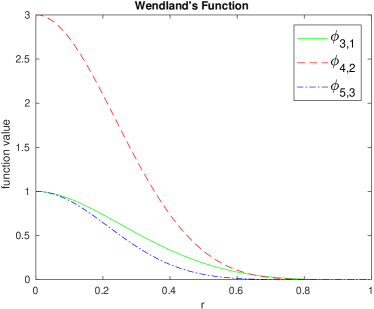
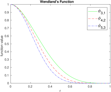
Figure 2: Wendland’s functions before and after scaling.

With these three components, we can apply local WLS fittings to construct a local surface patch at an arbitrary point of a triangulated surface or a piecewise linear curve. More specifically, consider a point $\boldsymbol{p}$ on a triangle $\boldsymbol{x}_{1}\boldsymbol{x}_{2}\boldsymbol{x}_{3}$. For each vertex $\boldsymbol{x}_{j}$, we find its $k$-ring neighborhood $S_{j}$. If $\boldsymbol{p}$ is on the edge $\boldsymbol{x}_{j_{1}}\boldsymbol{x}_{j_{2}}$, we use $S_{j_{1}}\bigcup S_{j_{2}}$ as the stencil; if $\boldsymbol{x}_{0}$ is in the interior of the triangle, we use $\bigcup_{j=1}^{3}S_{j}$ as the stencil. To build the local frame, we take $\sum_{j=1}^{3}\xi_{j}\boldsymbol{m}_{j}$ as an approximate normal, where $\boldsymbol{m}_{j}$ is the approximate normal at $\boldsymbol{x}_{j}$ and $\xi_{j}$ is the barycentric coordinates of $\boldsymbol{p}$ in the triangle. This construction ensures the local frames change continuously from point to point, and hence it is referred to as the Continuous Moving Frames (CMF) method [12]. If the input vertices approximate a smooth surface $\Gamma$ with an error of $\mathcal{O}(h^{p+1})$, it can be shown that the CMF reconstruction with degree-$p$ polynomials can achieve $\mathcal{O}(h^{p+1})$ accuracy, where $h$ is proportional to the radius of the stencil. For even-degree polynomials, the error may be $\mathcal{O}(h^{p+2})$ for symmetric stencils due to error cancellation. For this reason, it is in general advantageous to use even-degree polynomials.

2.4 Weighted Averaging of Local Fittings

The local WLS fittings and CMF do not necessarily produce a $G^{0}$ continuous surface. One approach to recover $G^{0}$ continuity is Weighted Averaging of Local Fittings (WALF) [12], which computes a weighted average of the local fittings at the vertices, where the weights are the barycentric coordinates. For example, consider a triangle with vertices $\boldsymbol{x}_{j}$, $j=1,2,3$, and an arbitrary point $\boldsymbol{p}$ in the triangle. For each vertex $\boldsymbol{x}_{j}$, a point $\boldsymbol{q}_{j}$ is obtained for $\boldsymbol{p}$ from the corresponding local fitting within its own local coordinate system. Let $\xi_{j}$, $j=1,2,3$ denote the barycentric coordinates of $\boldsymbol{p}$ within the triangle. Then, $\boldsymbol{q}=\sum_{j=1}^{3}\xi_{j}\boldsymbol{q}_{j}$ is the WALF reconstruction for $\boldsymbol{p}$. A similar construction also applies to curves. Figure 3 shows a 2-D illustration of this construction. For a smooth surface, WALF constructs a $G^{0}$ continuous surface, due to the $C^{0}$ continuity of finite-element interpolation. It can be shown that if the input vertices approximate a smooth surface $\Gamma$ with an error of $\mathcal{O}(h^{p+1})$, then WALF reconstruction with degree-$p$ polynomials can achieve $\mathcal{O}(h^{p+1}+h^{6})$ accuracy for $p\leq 6$ in terms of the shortest distance to the true surface [12].

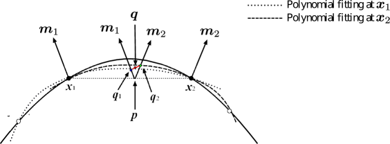
Figure 3: 2-D illustration of WALF. The solid curve indicates the exact curve. The dashed and dotted curves indicate the fittings at $\boldsymbol{x}_{1}$ and $\boldsymbol{x}_{2}$, respectively. $\boldsymbol{q}$ is the WALF reconstruction for point $\boldsymbol{p}$, computed as a weighted average of $\boldsymbol{q}_{1}$ and $\boldsymbol{q}_{2}$ from the fittings at $\boldsymbol{x}_{1}$ and $\boldsymbol{x}_{2}$, respectively.

2.5 High-Order Parametric Surface Elements

Besides WALF, another approach to obtain a $G^{0}$ continuous surface is to use high-degree piecewise polynomial interpolation, as in high-order finite-element methods. Specifically, for each triangle in the input mesh, one can construct a degree-$p$ surface patch from $n=(p+1)(p+2)/2$ points, including the three corner nodes in the original triangle, along with additional mid-edge nodes and mid-face nodes. Let $\{\boldsymbol{\xi}_{i}\}$ denote the natural coordinates of $\boldsymbol{x}_{i}$ in the reference space, which is typically chose as the right triangle with vertices $\boldsymbol{\xi}_{1}=[0,0]$, $\boldsymbol{\xi}_{2}=[1,0]$, and $\boldsymbol{\xi}_{3}=[0,1]$. Let $\boldsymbol{x}_{i}$ denote the coordinate of the $i$th node of the element. The degree-$p$ surface patch is then defined by

$$\boldsymbol{x}(\boldsymbol{\xi})=\sum_{i=1}^{n}N_{i}(\boldsymbol{\xi})\boldsymbol{x}_{i},$$ (17)

where the $N_{i}(\boldsymbol{\xi})$ are the Lagrange polynomial basis of degree-$p$ interpolation within the reference space, also know as the shape function of the degree-$p$ element. We refer to such a degree-$p$ triangular patch as a parametric surface element. It is commonly used in defining the geometry in high-order finite element methods, where $\boldsymbol{x}_{i}$ are sampling points on the exact geometry if a CAD is given. In the context of high-order reconstructions, the $\boldsymbol{x}_{i}$ corresponding to the mid-edge and mid-face nodes can be obtained from degree-$p$ CMF or WALF [12].

A key question in constructing a parametric surface element is the placement of the mid-edge and mid-face nodes. This includes two aspects: the selection of $\boldsymbol{\xi}_{i}$ for the mid-edge and mid-face nodes, and the placement of $\boldsymbol{x}_{i}$ based on $\boldsymbol{\xi}_{i}$. Traditionally, the $\boldsymbol{\xi}_{i}$ are equally spaced in the reference space, as illustrated in Figure 4 for degree-2, 4, and 6 triangles. For high-degree interpolation, such equally space points lead to ill-conditioned Vandermonde matrices and hence unstable Lagrange basis functions. For very high-degree interpolation, it is desirable to use nonuniform nodes that resemble the distributions of the Chebyshev points in 1-D for better stability. There are various choices for such points; see e.g. [16]. Among them, the Lebesgue-Gauss-Lobatto symmetric (LEBGLS) points, because they approximately minimize the condition number of the interpolation (a.k.a., the Lebesgue constant in the polynomial interpolation theory), and the points have a three-way symmetry. Hence, they are well suited for high-order surface reconstruction over triangular meshes. Figure 5 shows the LEBGLS points for degree-2, 4, and 6 triangles. Note that the degree-2 LEBGLS points are equally spaced, but those of higher-degrees tend to be more clustered toward the edges and corners. Given the points $\boldsymbol{\xi}_{i}$, the positioning of $\boldsymbol{x}_{i}$ requires special attention, especially near features, so that the derivatives of $\boldsymbol{x}(\boldsymbol{\xi})$ defined by (17) are uniformally bounded up to order $p+1$. We will address it in Section 5.

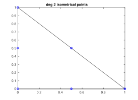
(a) degree 2

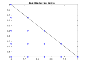
(b) degree 4

(c) degree 6

Figure 4: Parametric triangular elements with equally-spaced points in the reference space.

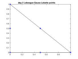
(a) degree 2

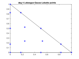
(b) degree 4

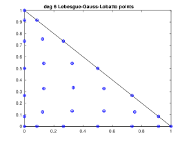
(c) degree 6

Figure 5: Parametric triangular elements with Lebesgue-Gauss-Lobatto points.

3 Hermite-Style High-Order Surface Reconstruction

The CMF and WALF methods in [12] had two main limitations. First, the methods may be inaccurate for relatively coarse meshes, for which the stencils may not have sufficient points and the safeguards would likely reduce the degree of the basis functions. Second, they do not guarantee $G^{0}$ continuity near sharp features (such as ridges and corners), which might be present in piecewise smooth surfaces. In this section, we address the first issue by extending CMF and WALF to include normal-based information, similar to Hermite interpolation. We refer to this as the Hermite-style reconstruction, and refer to its integrations with CMF and WALF as Hermite-style CMF (or H-CMF) and Hermite-style WALF (or H-WALF), respectively. We will describe these methods, including the selection of stencils and weighting schemes as well as the analysis of their accuracy.

3.1 Hermite-Style Polynomial Fittings

3.1.1 Local Polynomial Fittings.

Given a point $\boldsymbol{x}_{i}$ on a smooth surface $\Gamma$, let $\boldsymbol{n}_{i}$ denote an accurate normal to $\Gamma$ at $\boldsymbol{x}_{i}$. Note that unlike $\boldsymbol{m}_{i}$ in Section 2, which only needed to be first order, $\boldsymbol{n_{i}}$ should be at least $p$th order accurate for degree-$p$ fittings, as we will show in Section 3.3. Let $\boldsymbol{Q}_{0}^{T}\boldsymbol{n}=\left[\alpha_{i},\,\beta_{i},\,\gamma_{i}\right]^{T}$, where $\boldsymbol{Q}_{0}$ was defined in Section 2.1.1. From (2), we have

$$\gamma_{i}f_{u}(\boldsymbol{u}_{i}) =-\alpha_{i},$$ (18)

$$\gamma_{i}f_{v}(\boldsymbol{u}_{i}) =-\beta_{i}.$$ (19)

From the Taylor series expansion of $f(\boldsymbol{u})$ in (6), we have

$$f_{u}(\boldsymbol{u}_{i}) \approx\sum_{q=0}^{p}\sum_{j,k\geq 0}^{j+k=q}c_{jk}ju_{i}^{j-1}v_{i}^{k}\approx-\frac{\alpha_{i}}{\gamma_{i}},$$ (20)

$$f_{v}(\boldsymbol{u}_{i}) \approx\sum_{q=0}^{p}\sum_{j,k\geq 0}^{j+k=q}c_{jk}ku_{i}^{j}v_{i}^{k-1}\approx-\frac{\beta_{i}}{\gamma_{i}}.$$ (21)

These two equations along with the point-based approximation in (7) lead to the following linear system

$$\boldsymbol{U}\boldsymbol{c}\approx\boldsymbol{f},$$ (22)

where $\boldsymbol{c}$ is an $n$-vector composed of $c_{jk}$, $\boldsymbol{U}$ is a $3m\times n$ matrix, and $\boldsymbol{f}$ is a $3m$-vector. For example, a degree-2 fitting with $m$ points in the stencil results in the following $\boldsymbol{U}$ and $\boldsymbol{f}$:

$$\boldsymbol{U}=\left[\begin{array}[]{cccccc}1&u_{1}&v_{1}&u_{1}^{2}&u_{1}v_{1}&v_{1}^{2}\\ 1&u_{2}&v_{2}&u_{2}^{2}&u_{2}v_{2}&v_{2}^{2}\\ &\cdots&&&\cdots\\ 1&u_{m}&v_{m}&u_{m}^{2}&u_{m}v_{m}&v_{m}^{2}\\ 0&1&0&2u_{1}&v_{1}&0\\ 0&1&0&2u_{2}&v_{2}&0\\ &\cdots&&&\cdots\\ 0&1&0&2u_{m}&v_{m}&0\\ 0&0&1&0&u_{1}&2v_{1}\\ 0&0&1&0&u_{2}&2v_{2}\\ &\cdots&&&\cdots\\ 0&0&1&0&u_{m}&2v_{m}\end{array}\right]\quad\text{and}\quad\boldsymbol{f}=\left[\begin{array}[]{c}f_{1}\\ f_{2}\\ \vdots\\ f_{m}\\ -\alpha_{1}/\gamma_{1}\\ -\alpha_{2}/\gamma_{2}\\ \vdots\\ -\alpha_{m}/\gamma_{m}\\ -\beta_{1}/\gamma_{1}\\ -\beta_{2}/\gamma_{2}\\ \vdots\\ -\beta_{m}/\gamma_{m}\end{array}\right].$$ (23)

Like the regular fitting, the Hermite-style fitting is interpolatory at $\boldsymbol{x}_{0}$ if the local polynomial passes through the origin of fittings, i.e.,$f(\boldsymbol{u}_{0})=0$.

Note that if $\gamma_{i}\leq 0$, the local height function $f(\boldsymbol{u})$ would have foldings about $\boldsymbol{x}_{i}$, which can lead to non-convergence. This issue could be avoided by settings the weights for the folded vertices to zero so that they will be eliminated from the linear system; see Section 3.1.4. Also note that for surfaces with sharp features, the normals along ridges and at corners are not well-defined. In these cases, we can either use one-sided normals at each vertex on sharp features or do not include the normal information for those vertices. In the following, we shall assume the surface is smooth unless otherwise noted, so that the normal is well-defined at all the vertices in the stencil; we will address the reconstruction of feature curves in Section 4.

3.1.2 Coordinate Transformation Based on Geometric Scaling.

Due to the inclusion of normals into the Hermite-style fittings, the rows in (22) now have mixed-degree terms. To normalize the entries in matrix $\boldsymbol{U}$, we apply geometric scaling similar to that described in Section 2.2. Specifically, let $\mu=\dfrac{u}{h}$ and $\nu=\dfrac{v}{h}$, where $h$ is a measure of local edge length. From the chain rule, we have

$$\dfrac{\partial f^{j+k}}{\partial\mu^{j}\partial\nu^{k}}=\dfrac{\partial f^{j+k}}{\partial u^{j}\partial v^{k}}h^{j+k}.$$ (24)

Let $x_{jk}=h^{j+k}c_{ij}=\dfrac{1}{j!k!}\dfrac{\partial f^{j+k}(\boldsymbol{u}_{0})}{\partial\mu^{j}\partial\nu^{k}}$, $\mu_{i}=\dfrac{u_{i}}{h}$, and $\nu_{i}=\dfrac{v_{i}}{h}$ for $0\leq i\leq m$. From the Taylor series expansion of $f_{u}$ and $f_{v}$ in (20) and (21) , we obtain

$$\sum_{q=0}^{p}\sum_{j,k\geq 0}^{j+k=q}x_{jk}\mu_{i}^{j}\nu_{i}^{k} \approx f_{i},$$ (25)

$$\sum_{q=0}^{p}\sum_{j,k\geq 0}^{j+k=q}x_{jk}j\mu_{i}^{j-1}\nu_{i}^{k} \approx-\frac{\alpha_{i}}{\gamma_{i}}h,$$ (26)

$$\sum_{q=0}^{p}\sum_{j,k\geq 0}^{j+k=q}x_{jk}k\mu_{i}^{j}\nu_{i}^{k-1} \approx-\frac{\beta_{i}}{\gamma_{i}}h.$$ (27)

This results in a rescaled linear system

$$\boldsymbol{V}\boldsymbol{x}\approx\boldsymbol{g},$$ (28)

where $\boldsymbol{x}$ is an $n$-vector composed of $x_{jk}$, $\boldsymbol{V}$ is a $3m\times n$ matrix, and $\boldsymbol{g}$ is a $3m$-vector. For example, a degree-2 fitting results in the following $\boldsymbol{V}$ and $\boldsymbol{g}$:

$$\boldsymbol{V}=\left[\begin{array}[]{cccccc}1&\mu_{1}&\nu_{1}&\mu_{1}^{2}&\mu_{1}\nu_{1}&\nu_{1}^{2}\\ 1&\mu_{2}&\nu_{2}&\mu_{2}^{2}&\mu_{2}\nu_{2}&\nu_{2}^{2}\\ &\cdots&&&\cdots\\ 1&\mu_{m}&\nu_{m}&\mu_{m}^{2}&\mu_{m}\nu_{m}&\nu_{m}^{2}\\ 0&1&0&2\mu_{1}&\nu_{1}&0\\ 0&1&0&2\mu_{2}&\nu_{2}&0\\ &\cdots&&&\cdots\\ 0&1&0&2\mu_{m}&\nu_{m}&0\\ 0&0&1&0&\mu_{1}&2\nu_{1}\\ 0&0&1&0&\mu_{2}&2\nu_{2}\\ &\cdots&&&\cdots\\ 0&0&1&0&\mu_{m}&2\nu_{m}\end{array}\right]\quad\text{and}\quad\boldsymbol{g}=\left[\begin{array}[]{c}f_{1}\\ f_{2}\\ \vdots\\ f_{m}\\ -h\alpha_{1}/\gamma_{1}\\ -h\alpha_{2}/\gamma_{2}\\ \vdots\\ -h\alpha_{m}/\gamma_{m}\\ -h\beta_{1}/\gamma_{1}\\ -h\beta_{2}/\gamma_{2}\\ \vdots\\ -h\beta_{m}/\gamma_{m}\end{array}\right].$$ (29)

Mathematically, this geometric scaling is equivalent to multiplying the last $2m$ rows of (22) by $h$. In other words, $\boldsymbol{V}=\boldsymbol{D}\boldsymbol{U}\boldsymbol{T}$, where

$$\boldsymbol{D}=\left[\begin{array}[]{ccc}\boldsymbol{I}\\ &h\boldsymbol{I}\\ &&h\boldsymbol{I}\end{array}\right],$$ (30)

and $\boldsymbol{T}$ is the diagonal matrix composed of $h^{-j-k}$, where $j$ and $k$ are the powers in $\mu^{j}\nu^{k}$.

3.1.3 Stencil Selection.

The stencil selection is important for the accuracy and efficiency of the local polynomial fittings, since too large a stencil tends to cause overfitting, while too small a stencil leads to low order accuracy. A degree-$p$ polynomial fitting has $n=(p+1)(p+2)/2$ coefficients to determine, so it requires at least $n$ points in the stencil for point-based fittings. However, for Hermite-style fittings, there are three equations for each point: one from the vertex position, and two from the normal vector. Hence, Hermite-style fittings require much fewer points in the stencil. As described in Section 2.3, we choose the stencil of a vertex based on its $k$-ring neighborhood in $1/2$ increments. Table 1 shows a typical choice of ring size of point-based and Hermite-style fittings. In addition, the table also shows the average numbers of vertices in the rings for an example triangulation of a torus with 336 triangles. It can be seen that for the Hermite-style fittings, it typically suffices to use only a 1-ring neighborhood for degree-4 fittings, and only a 2-ring neighborhood for degree-6 fittings. These are much more compact than the typical 2.5-ring and 3.5-ring neighborhoods for the corresponding point-based fittings. Note that similar to the point-based fittings, if there are insufficient vertices in a stencil, our stencil selection procedure adaptively enlarges the ring sizes.

Table 1: Comparison of average stencil sizes for point-based and Hermite-style fittings.

	degree 2		degree 3		degree 4		degree 5		degree 6
#unknowns	6		10		15		21		28
	#ring	#vert	#ring	#vert	#ring	#vert	#ring	#vert	#ring	#vert
point-based	1.5	12.6	2	18.4	2.5	29.6	3	37.5	3.5	52.7
Hermite-style	1	6.8	1	6.8	1	6.8	1.5	12.6	2	18.4

Note that for points near sharp features, we must make sure not to cross a ridge curve when building the stencil. To this end, we virtually split the surface into smooth patches along the feature curves, and reconstruct each smooth patch independently. This is more robust, if the feature curves can be identified a priori from the CAD model or using some robust algorithms, such as that in [10]. For ridge curves with very large dihedral angles, one could also use the safeguard $\theta^{+}$ in the weighting scheme to filter out points for simplicity.

3.1.4 Weighting Scheme.

Similar to the point-based fittings, (28) can be solved under the framework of weighted linear least squares to minimize the weighted norm,

$$\min_{\boldsymbol{x}}\left\|\boldsymbol{\Omega}(\boldsymbol{Vx}-\boldsymbol{g})\right\|_{2}=\min_{\boldsymbol{c}}\left\|\boldsymbol{\Omega D}(\boldsymbol{Uc}-\boldsymbol{f})\right\|_{2},$$ (31)

where $\boldsymbol{\Omega}=\text{diag}(\omega_{1},\dots,\omega_{3m})$ is a $3m\times 3m$ weighting matrix, and $\boldsymbol{c}=\boldsymbol{T}\boldsymbol{x}$ for $\boldsymbol{c}$ and $\boldsymbol{T}$ defined in (22) and (30), respectively.

A key question is the selection of the weights. Let us first consider the first $m$ weights $\omega_{1},\dots,\omega_{m}$ corresponding to the equations (7). As described in Section 2.3, we construct the weights based on a combination of Wendland’s functions [21] and normal-based safeguards, Specifically, let

$$\omega_{i}=\theta_{i}^{+}\psi(\|\boldsymbol{u}_{i}\|/\rho),$$ (32)

where $\theta_{i}^{+}=\textrm{max}(0,\boldsymbol{m}_{i}^{T}\boldsymbol{m}_{0})$, $\rho$ is a measure of the radius of the stencil, and $\psi$ is a Wendland’s function. For even degrees $2,$ 4, and $6$, we use $\psi=\psi_{3,1}$, $\psi_{4,2}$, and $\psi_{5,3}$ as defined in (14)–(16), respectively; for odd degrees $p=2q-1$, we use the same weighting schemes as for degree $2q$. To compute $\rho$, we find the $k$th nearest neighbors of $\boldsymbol{x}_{0}$ in $uv$-plane within the stencil, where $k$ is chosen to be the ceiling of $1.5$ times the number of unknowns, i.e., $k=\left\lceil 0.75(p+1)(p+2)\right\rceil$, and then

$$\rho=c\|\boldsymbol{u}_{k}\|,$$ (33)

where $c>1$ depends on the degree of fitting. In particular, we choose $c=1.15$, $1.2$, and $1.25$ for degrees $2,$ 4, and $6$, respectively, which we obtained via numerical experimentation. For the equations corresponding to $f_{u}$ and $f_{v}$, since we have applied geometric scalings in (28), we apply the same weights $\omega_{i}$ to all the equations associated with points $\boldsymbol{u}_{i}$. In other words,

$$\boldsymbol{\Omega}=\begin{bmatrix}\boldsymbol{W}\\ &\boldsymbol{W}\\ &&\boldsymbol{W}\end{bmatrix}\quad\text{and}\quad\boldsymbol{\Omega}\boldsymbol{D}=\begin{bmatrix}\boldsymbol{W}\\ &h\boldsymbol{W}\\ &&h\boldsymbol{W}\end{bmatrix},$$ (34)

where $\boldsymbol{W}$ is composed of $\omega_{i}$ in (32). The resulting weighted Vandermonde system can then be solved using truncated QR with column pivoting as described in Section 2.2.

3.2 H-CMF and H-WALF

The Hermite-style polynomial fittings described above can be integrated into CMF and WALF, which refer to as H-CMF and H-WALF, correspondingly. H-CMF works similarly to CMF, as described in Section 2.3. In particular, it first constructs the local coordinate frame at point $\boldsymbol{p}$ in triangle $\boldsymbol{x}_{1}\boldsymbol{x}_{2}\boldsymbol{x}_{3}$ by averaging the approximate nodal normals $\boldsymbol{m}_{j}$ using the barycentric coordinates $\xi_{j}$. Then, the stencil for $\boldsymbol{p}$ is taken to be the union of the stencils of the three nodes. H-CMF does not guarantee $G^{0}$ continuity, because the weighting scheme may be discontinuous and there may be truncation when solving the least squares problems.

H-WALF works similarly to WALF, as described in Section 2.4. More specifically, consider a triangle composed of vertices $\boldsymbol{x}_{j}$, $j=1,2,3$. For any point $\boldsymbol{p}$ in the triangle, we first obtain a point $\boldsymbol{q}_{j}$ from the Hermite-style fitting in the local coordinate frame at $\boldsymbol{x}_{j}$. Let $\xi_{j}$, $j=1,2,3$ be the barycentric coordinates of $\boldsymbol{p}$ within the triangle. Then, the H-WALF reconstruction of $\boldsymbol{p}$ is given by $\boldsymbol{q}=\sum_{j=1}^{3}\xi_{j}\boldsymbol{q}_{j}$. For smooth surfaces, H-WALF constructs a $G^{0}$ continuous surface.

3.3 Accuracy of Hermite-Style Fittings

To analyze the accuracy of H-CMF and H-WALF, we must first understand the convergence of the Hermite-style polynomial fittings. This analysis is similar to the point-based fittings in [14], but the inclusion of the normals requires some special care. Hence, we include the analysis here for completeness. Assuming the mesh is relatively uniform, let h denote a measure of average edge length of the mesh. We obtain the following lemma.

Lemma 1.

Given a set of points $[u_{i},v_{i},\tilde{f}_{i}]$ that interpolate a smooth height function $f$ or approximate f with an error of $\mathcal{O}(h^{p+1})$, along with the gradients $[f_{u}(\boldsymbol{u}_{i}),f_{v}(\boldsymbol{u}_{i})]$, which are approximated to $\mathcal{O}(h^{p})$, assume that the point distribution and the weights are independent of $h$, and the condition number in any $p$-norm of the scaled matrix $\boldsymbol{\varOmega V}$ is bounded by some constant. Then, the degree-d weighted least squares fitting approximates $c_{jk}$ in (22) to $\mathcal{O}(h^{p-j-k+1})$.

Proof.

Consider the least squares problem (22). Let $\boldsymbol{A}=\boldsymbol{\Omega}\boldsymbol{V}=\boldsymbol{\varOmega DUT}$ and $\boldsymbol{b}=\boldsymbol{\Omega}\boldsymbol{g}$. Let $\hat{\boldsymbol{c}}$ denote the exact coefficients in the Taylor polynomial (5). Let $\hat{\boldsymbol{x}}=\boldsymbol{T}\hat{\boldsymbol{c}}$, $\hat{\boldsymbol{b}}=\boldsymbol{\Omega}\boldsymbol{V}\boldsymbol{x}$, $\delta\boldsymbol{x}=\boldsymbol{x}-\hat{\boldsymbol{x}}$, and $\boldsymbol{r}=\boldsymbol{b}-\hat{\boldsymbol{b}}$. Then, $\boldsymbol{A}\hat{\boldsymbol{x}}=\hat{\boldsymbol{b}}$, and $\delta\boldsymbol{x}$ is the least squares solution to

$$\boldsymbol{A}\delta\boldsymbol{x}\approx\boldsymbol{r}.$$ (35)

Hence,

$$\left\|\delta\boldsymbol{x}\right\|_{\infty}\leq\left\|\boldsymbol{A}^{+}\right\|_{\infty}\left\|\boldsymbol{r}\right\|_{\infty}.$$ (36)

Note that $\boldsymbol{r}=\boldsymbol{b}-\hat{\boldsymbol{b}}=\boldsymbol{\Omega}\boldsymbol{D}(\boldsymbol{f}-\boldsymbol{U}\hat{\boldsymbol{c}})$. Under the assumption that $f(\boldsymbol{u}_{i})$ is approximated to at least $\mathcal{O}(h^{p+1})$ and the derivatives $f_{u}(\boldsymbol{u}_{i})$ and $f_{v}(\boldsymbol{u}_{i})$ are approximated to $\mathcal{O}(h^{p})$, each entry in $\boldsymbol{D}(\boldsymbol{f}-\boldsymbol{U}\hat{\boldsymbol{c}})$ is $\mathcal{O}(h^{p+1})$, so is each entry in $\boldsymbol{r}$ since $\omega_{i}=\Theta(1)$. Under the assumptions of the theorem, $\kappa_{\infty}(\boldsymbol{A})=\left\|\boldsymbol{A}\right\|_{\infty}\left\|\boldsymbol{A}^{+}\right\|_{\infty}=\Theta(1)$ and $\left\|\boldsymbol{A}\right\|_{\infty}=\Theta(1)$. Hence, $\left\|\boldsymbol{A}^{+}\right\|_{\infty}=\Theta(1)$ and $\left\|\delta\boldsymbol{x}\right\|_{\infty}=\mathcal{O}(h^{p+1})$. Therefore, each entry in $\delta\boldsymbol{c}=\boldsymbol{T}\delta\boldsymbol{x}$ corresponding to $c_{ij}$ is $\mathcal{O}(h^{p-j-k+1})$. ∎

The accuracy of H-CMF directly follows from Lemma 1.

Proposition 2.

Given a mesh whose vertices approximate a smooth surface $\Gamma$ with an error of $\mathcal{O}(h^{p+1})$ and the normal vectors are also approximated to $\mathcal{O}(h^{p})$, assuming the rescaled Vandermonde systems are well conditioned, the distance between each point on the H-CMF reconstructed surface and its closest point on $\Gamma$ is $\mathcal{O}(h^{p+1})$.

Proof.

In H-CMF, the gradients to the local height function $f$ are $[-\alpha_{i}/\gamma_{i},-\beta_{i}/\gamma_{i}]$, where $\boldsymbol{Q}_{0}^{T}\boldsymbol{n}_{i}=[\alpha_{i},\beta_{i},\gamma_{i}]^{T}$. Since the normals are $p$th order accurate, so is the approximation to $f_{u}$ and $f_{v}$ as long as $\gamma_{i}$ is bounded away from 0. It then follows from Lemma 1 that the local height function is approximated to $\mathcal{O}(h^{p+1})$, so is the distance from the reconstructed point to the closest point on $\Gamma$. ∎

In Proposition 2, the well-conditioning of the Vandermonde system is typically achieved by the adaptive stencil selection. If the Vandermonde system is ill-conditioned, then some higher-order terms may be truncated by QRCP, and and the convergence rate may be lower. In the proof, it is important that $\gamma_{i}$ is bounded away from 0, which can be ensured by the normal-based safeguards in the weighting schemes.

The accuracy of H-WALF is more complicated, in that like WALF, its error has a lower bound $\mathcal{O}(h^{6})$. We summarize its convergence rate as follows.

Proposition 3.

Under the same assumption as Proposition 2, the distance between each point on the H-WALF reconstructed surface and its closest point on $\Gamma$ is $\mathcal{O}(h^{p+1}+h^{6})$.

The lower bound of $\mathcal{O}(h^{6})$ error is due to the discrepancies of the local coordinate frames at the vertices of a triangle. Figure 6 illustrates the origin of this error bound. Let $\boldsymbol{q}$ denote the H-WALF reconstruction of a point $\boldsymbol{p}$ in the triangle $\boldsymbol{x}_{1}\boldsymbol{x}_{2}\boldsymbol{x}_{2}$. Let $\bar{\boldsymbol{q}}^{*}$ be the closest point of $\boldsymbol{q}$ on $\Gamma$. Let $\boldsymbol{q}_{j}^{*}$ be projection of $\boldsymbol{p}$ onto the exact surface $\Gamma$ along $\boldsymbol{m}_{j}$, and $\boldsymbol{q}^{*}=\sum_{j=1}^{3}\xi_{j}\boldsymbol{q}_{j}^{*}$. Then

$$\text{dist}(\boldsymbol{q},\Gamma)\leq\parallel\boldsymbol{q}-\bar{\boldsymbol{q}}^{*}\parallel\leq\parallel\boldsymbol{q}-\boldsymbol{q}^{*}\parallel+\parallel\boldsymbol{q}^{*}-\bar{\boldsymbol{q}}^{*}\parallel.$$ (37)

The error $\parallel\boldsymbol{q}-\boldsymbol{q}^{*}\parallel=\mathcal{O}(h^{p+1})$ is due to Lemma 1. It can be shown that $\|\boldsymbol{q}_{i}^{*}-\boldsymbol{q}_{j}^{*}\|=\mathcal{O}(h^{3})$ for $1\leq i,j\leq 3$ and $\parallel\boldsymbol{q}^{*}-\bar{\boldsymbol{q}}^{*}\parallel=\mathcal{O}(\max\|\boldsymbol{q}_{i}^{*}-\boldsymbol{q}_{j}^{*}\|)^{2}=\mathcal{O}(h^{6})$; see [12] for a complete proof.

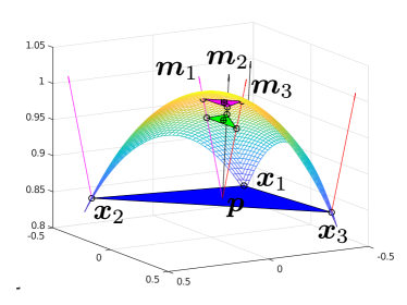
(a) An element and exact surface.

(b) Enlarged local view.

Figure 6: 3-D illustration of error analysis in H-WALF.

Finally, we note that in Lemma 1, for even-degree polynomials, the leading-error terms are odd-degree polynomials, which may result in error cancellation if the stencils are perfectly symmetric, analogous to the error cancellation in center-difference schemes. In practice, error cancellation also occurs for nearly symmetric stencils. Therefore, we may observe similar convergence rates for polynomial fittings of degrees $2q$ and $2q+1$. Furthermore, since degree-2$q$ fittings require smaller stencils, they may have even smaller errors than degree-($2q+1$) fittings. Hence, it is desirable to use even-degree polynomials for high-order reconstructions for nearly symmetric stencils, as we will demonstrate in Section 6. Furthermore, Propositions 2 and 3 imply that H-WALF is less accurate than H-CMF for high-degree polynomials. In practice, H-WALF is well suited for degree-2 or degree-4 reconstructions for its better efficiency, and H-CMF is better suited for degree-6 or higher-order reconstructions. In addition, we note that H-CMF tends to deliver better stability than H-WALF if the stencil is one-sided, and hence for open surfaces or piecewise smooth surfaces, H-CMF is preferred near boundaries or sharp features.

4 Hermite-Style High-Order Curve Reconstruction

In this section, we present a procedure for high-order reconstruction of space curves, such as feature curves on a piecewise smooth surface or the boundary curve of an open surface. We focus on Hermite-style reconstruction using points and tangents, which can be simplified to point-based reconstruction if one omits the equations associated with tangents. We assume the curve is piecewise smooth, and its end-points or corners are accurate and do not need reconstruction.

4.1 H-CMF and H-WALF Curve Reconstructions

Consider a point $\boldsymbol{x}_{0}$ and a collection of points $\{\boldsymbol{x}_{i}\mid 1\leq i\leq m\}$ in its neighborhood on a curve. Let $\boldsymbol{t}_{i}$ denote an accurate tangent vector to the curve at $\boldsymbol{x}_{i}$. Let $u_{i}$ denote the local coordinate of $\boldsymbol{x}_{i}$ in the local $uvw$ frame centered $\boldsymbol{x}_{0}$ as defined in Section 2.1.2, and let $\boldsymbol{Q}_{0}^{T}(\boldsymbol{x}_{i}-\boldsymbol{x}_{0})=\left[u_{i},v_{i},w_{i}\right]^{T}$. Let $\boldsymbol{f}$ denote the vector-valued local height function. The Taylor series of $\boldsymbol{f}$ about $u_{0}=0$ is given by

$$\boldsymbol{f}(u)\approx\stackrel{{\scriptstyle[}}{{q}}=0]{p}{\sum}\boldsymbol{c}_{q}u^{q}$$ (38)

where $\boldsymbol{c}_{q}=\dfrac{1}{q!}\dfrac{d^{q}}{du^{k}}\boldsymbol{f}(u_{0})$. Let $c_{q}$ and $d_{q}$ denote the two entries in $\boldsymbol{c}_{q}$, respectively. For each point $\boldsymbol{x}_{i}$, we then have two equations

$$\stackrel{{\scriptstyle[}}{{q}}=0]{p}{\sum}c_{q}u_{i}^{q}\approx u_{i},$$ (39)

$$\stackrel{{\scriptstyle[}}{{q}}=0]{p}{\sum}d_{q}u_{i}^{q}\approx w_{i}.$$ (40)

This amounts to a $2m\times n$ linear system for point-based curve reconstruction, where $n=p+1$.

For Hermite-style reconstruction, let $\boldsymbol{Q}_{0}^{T}\boldsymbol{t}_{i}=\left[\alpha_{i},\beta_{i},\gamma_{i}\right]^{T}$, and then $\boldsymbol{f}^{\prime}(u_{i})=\left[\dfrac{\beta_{i}}{\alpha_{i}},\dfrac{\gamma_{i}}{\alpha_{i}}\right]^{T}$. The Taylor series of $\boldsymbol{f}^{\prime}$ about $u_{0}=0$ is given by

$$\boldsymbol{f}^{\prime}(u) \approx\stackrel{{\scriptstyle[}}{{q}}=1]{p}{\sum}q\boldsymbol{c}_{q}u^{q-1}.$$ (41)

For the given tangent vector at vertex $\boldsymbol{x}_{i}$, we then have two additional equations

$$\stackrel{{\scriptstyle[}}{{q}}=1]{p}{\sum}qc_{q}u_{i}^{q-1}\approx\dfrac{\beta_{i}}{\alpha_{i}},$$ (42)

$$\stackrel{{\scriptstyle[}}{{q}}=1]{p}{\sum}qc_{q}u_{i}^{q-1}\approx\dfrac{\gamma_{i}}{\alpha_{i}}.$$ (43)

Assuming a tangent vector is given for each point $\boldsymbol{x}_{i}$, we obtain a $4m\times n$ linear system for Hermite-style curve reconstruction. For curves with corners, the tangent direction at a corner may not be well-defined. In this case, we can either use one-sided tangent at a corner, or do not include the equations associated with the tangents at corners.

On a triangulated surface, a feature curve is composed of edges. In general, we choose the stencil to be the $\left\lceil(p+1)/2\right\rceil$ and $\left\lceil(p+1)/4\right\rceil$ rings for the point-based and Hermite-style reconstructions, respectively, and we adaptively enlarge the ring sizes if there are insufficient number of points. We use the Wendland weights with safeguards, as described in Section 3.1, except that safeguard $\theta_{i}^{+}$ are now defined based on tangents instead of normals. The resulting weighted least squares problem is then rescaled geometrically and solved robustly using QRCP.

By defining a $C^{0}$ continuous tangent vector field on a feature curve, we obtain the CMF and H-CMF local reconstructions. To recover a $G^{0}$ continuous curve, we can utilize the weighted averaging of the local reconstructions at the vertices to obtain WALF and H-WALF reconstructions. Alternatively, we can use high-order parametric elements to define a $G^{0}$ continuous curve. These constructions are similar to their counterparts for surfaces as described in Section 3, and hence we omit their details.

4.2 Accuracy of Curve Reconstructions

Let h denote the average edge length of the mesh. Then, the following lemma can be established:

Lemma 4.

Given a set of points $[u_{i},v_{i},w_{i}]$ that interpolate a smooth curve or approximate the curve with an error of $\mathcal{O}(h^{p+1})$, along withe the derivatives $v^{\prime}(u_{i})$ and $w^{\prime}(u_{i})$, which are approximated to $\mathcal{O}(h^{p})$, assume the point distribution and the weights are independent of $h$, and the condition number of the scaled matrix $\boldsymbol{\varOmega V}$ is bounded by some constant. The degree-d weighted least squares fitting approximates $c_{q}$ and $d_{q}$ to $\mathcal{O}(h^{p-q+1})$.

The proof of this lemma is similar to that of Lemma 1. The key in the proof is that after geometric scaling, the component in the residual vector is $\Theta(1)$, so is the perturbation to the solution vector. Undoing the geometric scaling, we bound the perturbations to $c_{q}$ and $d_{q}$ by $\mathcal{O}(h^{p-q+1})$.

The accuracy of H-CMF of curve reconstruction directly follows from Lemma 4.

Proposition 5.

Given a piecewise linear curve, whose vertices approximate a smooth curve $\gamma$ with an error of $\mathcal{O}(h^{p+1})$ and the tangents are approximated to $\mathcal{O}(h^{p})$, assuming the rescaled Vandermonde systems are well conditioned, the distance between each point on the H-CMF reconstruction with degree-p fittings and its closest point on $\gamma$ is $\mathcal{O}(h^{p+1})$.

The result in Proposition 5 also holds for CMF reconstruction. However, the accuracy of H-WALF curve reconstruction is also bounded by $h^{6}$, similar to surface reconstructions.

Proposition 6.

Under the same assumption as Proposition 5, the distance between each point on the H-WALF reconstruction of a smooth curve $\gamma$ with degree-p fittings and its closest point on $\gamma$ is $\mathcal{O}(h^{p+1}+h^{6})$.

The same result holds for WALF reconstruction. The bound of $h^{6}$ is due to the discrepancy of local coordinate systems at the two vertices of an edge; we omit the proof here.

4.3 $G^{0}$ Continuity of H-WALF Reconstruction

It is clear that for smooth curves, $G^{0}$ continuity is guaranteed by H-WALF (and WALF) curve reconstructions. For piecewise smooth curves, some care must be taken. First, when selecting stencils for points near a corner, we must make sure not to select points across a corner. This can be done by virtually splitting the curves at the corners into smooth segments, and then reconstructing each smooth segment independently. Alternatively, we can use the safeguard $\theta^{+}$ in the weighting scheme to filter out points whose tangent directions have a large angle against that at the origin. Second, at a corner $\boldsymbol{x}_{0}$, we need to construct a local fitting within each edge incident on $\boldsymbol{x}_{0}$ using the one-sided tangent as $\boldsymbol{s}_{0}$ for constructing the local frame. Third, if a corner has more than two incident edges, we must enforce the local fit within each of its incident edges to be interpolatory at $\boldsymbol{x}_{0}$, so that all the reconstructed curves would meet at $\boldsymbol{x}_{0}$. Under this construction, H-WALF can deliver accurate $G^{0}$ continuous reconstructions for piecewise smooth curves.

5 Iterative Feature-Aware Parametric Surfaces Reconstruction

The preceding two sections focused on the reconstructions of smooth surfaces and of feature curves on a piecewise smooth surface, respectively. In this section, we combine the two techniques to reconstruct a piecewise smooth surface to high-order accuracy with guaranteed $G^{0}$ continuity. It is challenging to achieve both accuracy and continuity simultaneously. For example, WALF (or H-WALF) does not guarantee continuity along sharp features. This is because the reconstructed feature curves in general do not match with the edges of the reconstructed surface patches in their incident triangles. This is illustrated in Figure 7, where the curve reconstruction of feature edge $\boldsymbol{v}_{1}\boldsymbol{v}_{2}$ may have a different shape than the corresponding edge in the surface reconstructions of triangles $\boldsymbol{v}_{1}\boldsymbol{v}_{2}\boldsymbol{v}_{3}$ and $\boldsymbol{v}_{1}\boldsymbol{v}_{2}\boldsymbol{v}_{4}$. A linear combination of the reconstructed curve and the reconstructed surfaces can recover continuity but may compromise the convergence rate. Similarly, the parametric surface elements described in Section 2.5 can recover continuity, but they may not deliver optimal convergence rate near sharp features. In this section, we propose an iterative procedure to construct parametric elements, which achieves both accuracy and continuity.

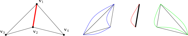
Figure 7: The lack of continuity between the WALF reconstructed feature edge and the WALF-reconstructed surface patches in incident triangles.

5.1 Accuracy and Stability of Parametric Surfaces

The parametric elements in Section 2.5 provide a viable approach for reconstructing $G^{0}$ continuous surfaces. The key issue is the placement of the mid-edge and mid-face nodes. In general, this is a two-step procedure: first, define some intermediate position $\boldsymbol{p}_{i}$ for each node; second, project $\boldsymbol{p}_{i}$ onto $\boldsymbol{x}_{i}$ using high-order reconstruction or onto the exact surface if available. Both steps can affect the accuracy and the convergence rate of the reconstructed surface. However, the importance of the first step is more complicated and often overlooked. In the following, we analyze the impact of both steps, with an emphasis on the first step.

Consider a degree-$p$ element with $n$ nodes. Let $\boldsymbol{\xi}_{i}$ denote the natural coordinates of the $i$th node of the element. Without loss of generality, we shall assume the nodes are composed of LESGLS points. Let $\boldsymbol{\xi}$ be the natural coordinates of point $\boldsymbol{x}(\boldsymbol{\xi})$, as defined in (17). Let $\Pi$ denote the projection from the intermediate points $\boldsymbol{p}_{i}$ onto $\boldsymbol{x}_{i}$, and then

$$\boldsymbol{x}(\boldsymbol{\xi})=\sum_{i=1}^{n}N_{i}(\boldsymbol{\xi})\boldsymbol{x}_{i}=\sum_{i=1}^{n}N_{i}(\boldsymbol{\xi})\Pi(\boldsymbol{p}_{i}).$$ (44)

For $\boldsymbol{x}(\boldsymbol{\xi})$ to be accurate, it is important that it is smooth to degree $p+1$ in the following sense.

Definition 7.

The parameterization $\boldsymbol{x}(\boldsymbol{\xi})$ is smooth to degree $q$ if the partial derivatives of $\boldsymbol{x}$ with respect to $\boldsymbol{\xi}$ are uniformally bounded up to $q$th order.

The correlation of the smoothness and the accuracy of the parametric surface is established by the following theorem.

Theorem 8.

Given a smooth surface $\Gamma$ that is continuously differentiable to order $p+1$, assume the parameterization in (44) is smooth to degree $p+1$, the nodes $\boldsymbol{x}_{j}$ are reconstructed using degree-p H-CMF (or CMF), and the interpolation over the parametric element is stable. The reconstructed parametric surface approximates $\Gamma$ to $\mathcal{O}(h^{p+1})$, where $h$ is a characteristic length measure of the local stencil.

Proof.

Let $\hat{\boldsymbol{x}}(\boldsymbol{\xi})$ denote the closest point to $\boldsymbol{x}(\boldsymbol{\xi})$ on $\Gamma$, and $\hat{\boldsymbol{x}}_{i}$ the closest point to $\boldsymbol{x}_{i}$ on $\Gamma$. Then,

$$\left\|\boldsymbol{x}(\boldsymbol{\xi})-\hat{\boldsymbol{x}}(\boldsymbol{\xi})\right\| =\left\|\sum_{i=1}^{n}N_{i}(\boldsymbol{\xi})\Pi(\boldsymbol{p}_{i})-\hat{\boldsymbol{x}}(\boldsymbol{\xi})\right\|$$ (45)

$$\leq\left\|\sum_{i=1}^{n}N_{i}(\boldsymbol{\xi})\hat{\boldsymbol{x}}_{i}-\hat{\boldsymbol{x}}(\boldsymbol{\xi})\right\|+\left\|\sum_{i=1}^{n}N_{i}(\boldsymbol{\xi})\left(\Pi(\boldsymbol{p}_{i})-\hat{\boldsymbol{x}}_{i}\right)\right\|.$$ (46)

With degree-$p$ CMF or H-CMF, the second term is $\mathcal{O}(h^{p+1})$, because

$$\left\|\sum_{i=1}^{n}N_{i}(\boldsymbol{\xi})\left(\Pi(\boldsymbol{p}_{i})-\hat{\boldsymbol{x}}_{i}\right)\right\|\leq\left(\sum_{i=1}^{n}\left|N_{i}(\boldsymbol{\xi})\right|\right)\max_{i}\left\|\left(\Pi(\boldsymbol{p}_{i})-\hat{\boldsymbol{x}}_{i}\right)\right\|=\mathcal{O}(h^{p+1}),$$ (47)

and $\sum_{i=1}^{n}\left|N_{i}(\boldsymbol{\xi})\right|=\mathcal{O}(1)$ for stable elements. From the Taylor series, and in particular the mean-value forms of its remainder, we can bound the first term in (46) by

$$\left\|\sum_{i=1}^{n}N_{i}(\boldsymbol{\xi})\hat{\boldsymbol{x}}_{i}-\hat{\boldsymbol{x}}(\boldsymbol{\xi})\right\|\leq\sum_{j,k\geq 0}^{j+k=p+1}\left\|\frac{\partial^{p+1}\boldsymbol{x}}{\partial\xi^{j}\partial\eta^{k}}\right\|_{\infty}\left|\xi^{j}\eta^{k}\right|.$$ (48)

Under the smoothness assumption, $\left\|\dfrac{\partial^{p+1}\boldsymbol{x}}{\partial\xi^{j}\partial\eta^{k}}\right\|_{\infty}=\mathcal{O}(1)$, so $\left\|\boldsymbol{x}(\boldsymbol{\xi})-\hat{\boldsymbol{x}}(\boldsymbol{\xi})\right\|=\mathcal{O}(h^{p+1})$. ∎

Theorem 8 still holds if we replace the H-CMF reconstruction with the exact surface, because the error in the first term in (46) is still bounded by $\mathcal{O}(h^{p+1})$. We could also use H-WALF (or WALF) for reconstruction, but it is undesirable because the error would be bounded by $\mathcal{O}(h^{6})$, and it is less stable than H-CMF due to the one-sided stencils near sharp features.

There are two key assumptions in Theorem 8. First, the interpolation must be stable, in that $\sum_{i=1}^{n}\left|N_{i}(\boldsymbol{\xi})\right|$ is bounded, ideally by a small constant. This may not hold for high-degree elements with equally space nodes, but this assumption is valid for elements with LESGLS nodes. Second, it assumes that $\boldsymbol{x}(\boldsymbol{\xi})$ is smooth to degree $p-1$ in order to bound the interpolation error in (48). This assumption requires some special attention in selecting the intermediate points $\boldsymbol{p}_{i}$ near features, as we discuss next.

5.2 Smoothness of Parameterization Near Features

When reconstructing high-order surfaces from a surface triangulation, a somewhat standard approach is to project the mid-edge and mid-face nodes in the piecewise linear triangle onto the exact surface or a high-order surface reconstruction. In other words,

$$\boldsymbol{p}_{i}=\sum_{j=1}^{3}N_{j}^{(1)}(\boldsymbol{\xi}_{i})\boldsymbol{x}_{j}^{(1)},\qquad 1\leq i\leq n$$ (49)

serve as the intermediate points, where the $N_{j}^{(1)}$ denote the shape functions of the linear elements and the $\boldsymbol{x}_{j}^{(1)}$ are the coordinates of the vertices of the triangle. Here, we shall focus on the analysis of these intermediate points, and we will assume that the projection $\boldsymbol{x}_{i}=\Pi\boldsymbol{p}_{i}$ is onto the exact surface, so that the second term in (46) is 0.

Near sharp features, the intermediate points in (49) can lead to nonsmooth parameterizations, if the projection $\Pi$ cause some abrupt contraction of the mid-edge and the mid-face nodes. This can happen if the geometry is the union of two spheres that intersect along a feature curve, as illustrated in Figure 8(a). We refer to this feature curve as a bubble-junction curve, because the union of the two spheres resemble the envelop of a double bubble. Consider a triangle incident on the feature curve. In Figure 8(b), we illustrate the projections of the mid-edge nodes of a degree-6 triangle along the left edge onto the exact circle, and the projections of the other nodes onto the exact sphere. Due to the discontinuity of the normal directions, the mid-edge nodes on the feature curve and the adjacent mid-face nodes contract toward each other abruptly. Figure 8(c) shows the contour plot of the inverse area measure, i.e. $1\left/\sqrt{\boldsymbol{J}^{T}\boldsymbol{J}}\right.$, where $\boldsymbol{J}$ denote the Jacobian matrix of $\boldsymbol{x}(\boldsymbol{\xi})$. The inverse area measure is clearly much larger near the feature curve. This non-uniformity can lead to large higher-order derivatives, and it worsen as the degree of the polynomial increases. Hence, the convergence rate using high-degree fittings may be compromised, as we will demonstrate in Section 6.

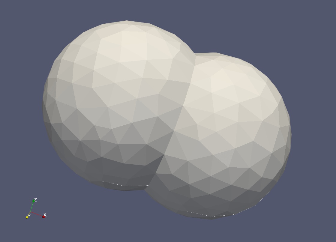
(a) Double sphere.

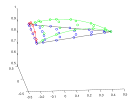
(b) Mid-edge and mid-face points.

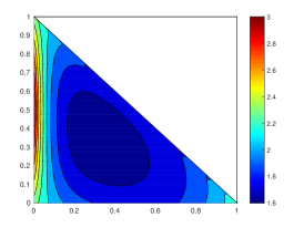
(c) Inverse area measure.

Figure 8: Nonsmooth parameterization near a bubble-junction feature.

One might attempt to improve the smoothness of $\boldsymbol{x}(\boldsymbol{\xi})$ by using some optimization procedure, but it would be difficult because $\Pi$ is discontinuous near sharp features and ensuring high-degree continuity may require the consideration of high-order derivatives in the objective function. Instead, we can improve the smoothness by an explicit construction of the intermediate points $\boldsymbol{p}_{i}$ using intermediate-degree polynomial interpolation. Specifically, let

$$\boldsymbol{p}_{i}=\sum_{j=1}^{n^{(q)}}N_{j}^{(q)}(\boldsymbol{\xi}_{i})\boldsymbol{x}_{j}^{(q)},\qquad 1\leq i\leq n,$$ (50)

where $N_{j}^{(q)}$ and $n^{(q)}$ are the shape functions and the number of nodes of degree-$q$ elements, respectively, where $1<q<p$, and $\boldsymbol{x}_{j}^{(q)}$ are the nodes of degree-$q$ elements that have taken into account the curved feature edges. For example, in the double-sphere example above, we use a quadratic element (i.e., $q=2$) to construct the intermediate points. Figure 9(a) shows the intermediate positions of the quadratic element, and Figure 9(b) shows the projection of these intermediate points onto the exact curve and surface. From the contour plot of the inverse area measure in Figure 9(c), it is clear that this new parameterization is much smoother than that in Figure 8. We can apply this idea iteratively to achieve higher-degree smoothness, as we describe next.

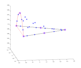
(a) Intermediate points.

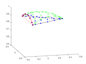
(b) Projected points.

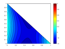
(c) Inverse area measure.

Figure 9: Smoother parameterization by constructing intermediate points using quadratic elements.

5.3 Iterative Feature-Aware Parameterization

The two-level construction in Figure 9 improves the uniformity of the area measure, which contain information of only first-order derivatives. To achieve higher-degree smoothness, we use multiple levels of intermediate nodes. Specifically, for each triangle incident on a feature (boundary) curve, we use a degree-$q$ interpolation to define its intermediate nodes, where

$$q=2^{\left\lceil\log p\right\rceil-1}.$$ (51)

The nodes $\boldsymbol{x}_{j}^{(q)}$ for the degree-$q$ element in (50), especially the mid-edge nodes on feature edges and the mid-face nodes, are computed recursively using degree $2^{\left\lceil\log q\right\rceil-1}$ interpolation. We refer to this procedure as Iterative Feature Aware (IFA) parameterization. The exponential decrease of the degree is due to the observation that the projection from the intermediate nodes from degree-$q$ interpolation introduces an $\mathcal{O}(h^{2q+2})$ perturbation to the parameterization.

In summary, the overall algorithm for constructing a degree-$p$ parametric surface proceeds as follows. First, use degree-$p$ H-CMF (or H-WALF if $p\leq 4$) to compute the mid-edge and mid-face nodes of degree-$p$ elements for all the triangles without a feature or border edge. Then for each element with a feature or border edge, we apply IFA parameterization to obtain its mid-edge and mid-face nodes. Finally, we use the nodes in the original input mesh along the mid-edge and mid-face nodes to define a $G^{0}$ continuous degree-$p$ parametric surface of guaranteed $(p+1)$st order accuracy.

An important application of this parametric surface is high-order finite element methods. In that setting, it is also important for the elements in the volume mesh (i.e., the tetrahedra) to have smooth parameterizations near boundaries. The IFA parameterization described here can be adapted to placing the mid-face and mid-cell nodes in these tetrahedra, which can improve the accuracy of FEM, as we demonstrate in Section 6.3. These IFA parameterizations may seem expensive for individual elements. However, this extra cost is negligible, because the number of elements incident on sharp features or the boundary is lower order compared to the total number of elements, due to the surface-to-volume ratio.

6 Numerical Results

In this section, we assess the proposed high-order reconstruction numerically, with a focus on the improved accuracy due to the Hermite-style fittings as well as iterative feature-aware parameterization. In addition, we also evaluate the effectiveness of the high-order reconstruction as an alternative of the exact geometry for high-order FEM. We will evaluate the methods using two surfaces, including the double sphere in Figure 8(a) and a torus in Figure 10(a). To evaluate curve reconstruction, we consider a conical helix in Figure 10(b), with the parametric equations

$$\boldsymbol{r}(t)=(t\cos(6t),t\sin(6t),t),\>(0\leqslant t\leqslant 2\pi).$$ (52)

Although simple, these geometries are representative of piecewise surfaces with different curvatures and sharp features.

To evaluate the convergence rates, we generate a series of triangular meshes for each geometry using mesh refinement and compute the pointwise error as the distance between a reconstructed point and its closest point on the exact surface or curve. Given an error vector $\boldsymbol{e}$ with $n$ points, we use a normalized $l_{2}$-norm of $\boldsymbol{e}$, computed as the standard vector $2$-norm by $\sqrt{n}$, i.e.,

$$\left\|\boldsymbol{e}\right\|_{\ell_{2}}=\frac{\left\|\boldsymbol{e}\right\|_{2}}{\sqrt{n}}=\sqrt{\frac{\sum_{i=1}^{n}e_{i}^{2}}{n}}.$$ (53)

Given a series of $k$ meshes, let $\boldsymbol{e}_{i}$ denote the error vector on the $i$th meshes and $n_{i}$ denote the number of points in the $i$th mesh, where level-1 denotes the coarsest mesh. The average convergence rate in $\ell_{2}$-norm is then computed as

$$\text{convergence rate}=d\frac{\log(\left\|\boldsymbol{e}_{1}\right\|_{\ell_{2}}/\left\|\boldsymbol{e}_{k}\right\|_{\ell_{2}})}{\log(n_{k}/n_{1})},$$ (54)

where $d=1$, 2, and $3$ for curve, surface, and volume meshes, respectively.

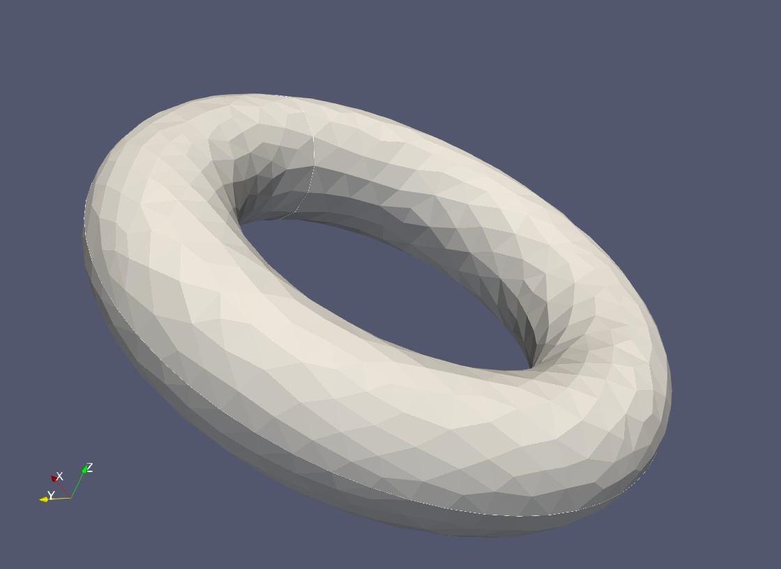
(a) Torus.

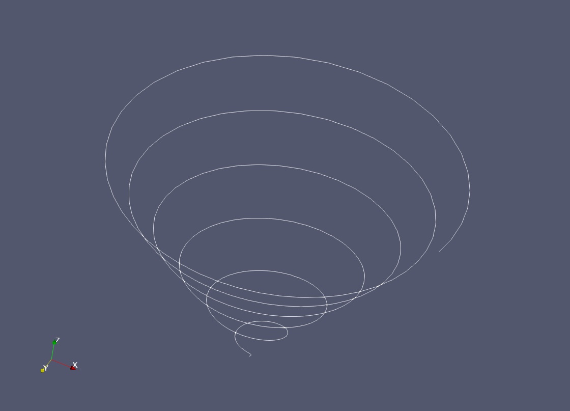
(b) Conical helix.

Figure 10: Test geometries for convergence studies.

6.1 Point-Based vs. Hermite-Style Reconstructions

We first assess the accuracy of point-based and Hermite-style surface reconstructions. As a base case, we use the double-sphere geometry, which was obtained by intersecting two unit spheres centered at the origin and at $[0.5,0.0]^{T}$, respectively. We generated three meshes using Gmsh [6] with 351, 1,402 and 5,598 vertices, respectively. We evaluate the convergence of CMF, WALF, H-CMF and H-WALF of degrees 2–7 with IFA parameterization. Figure 11 plots the $l_{2}$-norm of pointwise errors sampled at degree-6 Gaussian quadrature points, where the numbers to the right of the plots are the average convergence rates.

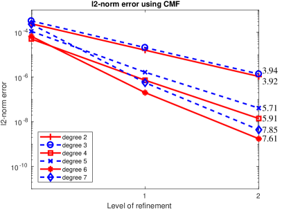
(a)

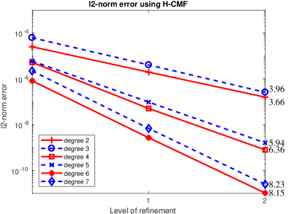
(b)

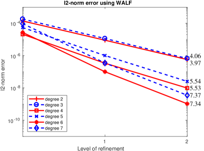
(c)

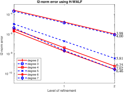
(d)

Figure 11: Comparison of point-based and Hermite-style surface reconstructions on double sphere.

We make a few observations about this result. First and foremost, for all the cases, the degree-$2q$ fittings are more accurate than the degree-$(2q+1)$ fittings. This is because the leading error terms of the even-degree polynomial fittings are odd degrees, which can cancel out for nearly symmetric meshes and nearly symmetric geometries. This leads to superconvergence for even-degree reconstructions. Furthermore, the degree-$2q$ fittings require smaller stencils than degree-$(2q+1)$ fittings, so they are both more accurate and more efficient. Hence, in the following tests we will consider only even-degree fittings.

Second, the Hermite-style reconstructions produced much smaller errors than their point-based counterparts with quartic and sextic polynomials, due to the more compact stencils and hence smaller constant factors in the errors. This demonstrates the benefits of Hermite-style reconstruction. These benefits are even more pronounced on coarsest meshes. Third, H-CMF and H-WALF had comparable accuracy for degree-4 fittings, but H-CMF significantly outperformed H-WALF for degree-6 fittings. Hence, H-CMF is preferred for sextic or higher-degree fittings for its superior accuracy, but H-WALF is preferred for quartic or lower-degree fittings for its comparable accuracy and better efficiency.

The above observations are consistent with our theoretical analysis in the preceding sections. We can also draw similar conclusions for surface reconstruction of nonuniform geometrics (such as a torus) as well as curve reconstructions (such as for a helix). Figure 12 shows the convergence results of surface reconstruction for the torus, where the three meshes have 898, 3,592, and 14,368 vertices, respectively. Figure 13 shows the convergence results of curve reconstruction for the helix, where the three meshes have 256, 512, and 1,024 vertices, respectively. It is clear that (1) even-degree fittings enjoyed superconvergence, (2) Hermite-style fittings outperformed their point-based counterparts for quartic and sextic fittings by one to two orders of magnitude, and (3) H-CMF significantly outperforms H-WALF for degree-6 reconstructions. However, note that point-based and Hermite-style reconstructions with quadratic polynomials had comparable results for smooth surfaces, because they have similar ring sizes. This behavior is different from that for the double sphere in Figure 11, for which the Hermite-style reconstruction enabled smaller one-sided stencils near sharp features and hence better accuracy even for quadratic polynomials.

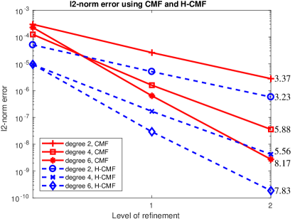
(a)

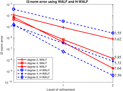
(b)

Figure 12: Comparison of point-based and Hermite-style surface reconstructions on the torus.

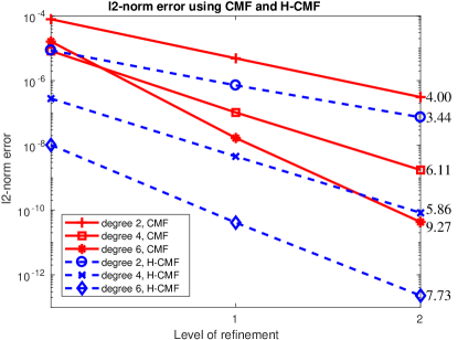
(a)

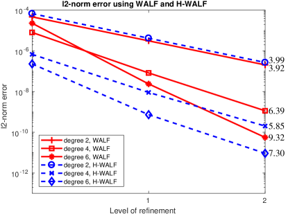
(b)

Figure 13: Comparison of point-based and Hermite-style curve reconstructions for the conical helix.

6.2 Benefits of IFA Parameterizations.

In Section 5.3, we introduced the iterative feature-aware (IFA) parameterization. To demonstrate its effectiveness, we compare the reconstruction of the double-sphere and the half-sphere geometries using CMF and H-CMF, with three different parameterizations:

• Non-FAP: Projecting the mid-edge and mid-face nodes from the linear triangle, as illustrated in Figure 8;

• FAP: Using quadratic element to construct intermediate nodes, as illustrated in Figure 9;

• IFAP: Using multiple levels of intermediate nodes with exponential growth of the degree, as described in Section  5.3.

Since our focus is for feature awareness, we consider only the elements incident on sharp features when computing the $l_{2}$-norm errors. Figure 14 shows the convergence rates of degree-6 CMF and H-CMF. To demonstrate the benefit of IFAP for higher-degree fittings, we also show the convergence results with degree-8 CMF and H-CMF for the two finer meshes. It is clear that FAP and IFAP outperformed non-FAP in all cases. IFAP outperformed FAP significantly for degree-8 H-CMF, although they performed similarly for the other cases.

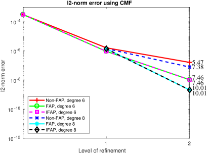
(a)

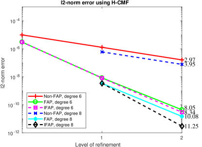
(b)

Figure 14: Convergences of CMF with no Non-FAP, FAP and IFAP for double sphere.

6.3 Application to High-Order FEM

Finally, we demonstrate the application of high-order surface reconstruction to high-order FEM with curved geometries. It is well known that linear FEM can deliver second-order convergence rates. High-order FEM uses higher-degree basis functions to approximate the solutions. However, these methods may fail to deliver high-order convergence rates if the curved boundaries are not approximated to at least the same order of accuracy. Hence, high-order surface reconstruction can play an important role for these problems.

To demonstrate the effectiveness of high-order surface reconstruction, we solve the Poisson equation with Dirichlet boundary conditions on the double-sphere geometry with the analytical solution

$$u(x,y,z)=e^{(x-0.5)^{2}+y^{2}+z^{2}}.$$ (55)

When the boundary representation is inexact, we set the boundary condition to the numerical values at the closest points on the exact surface. This is because the boundary condition are often available only on the exact surface geometry. To generate the high-order meshes for the problem, we start with a series of linear tetrahedral mesh with 1,455, 11,640, and 93,120 tetrahedra, respectively, and then add mid-edge, mid-face, and mid-cell nodes to the linear tetrahedra. The mid-edge and mid-face nodes on the surfaces are reconstructed using H-CMF with IFA parameterization. For the tetrahedra incident on the boundary, we first reconstruct their mid-face and mid-cell nodes also using IFA parameterization, as mentioned in Section 5.3. We consider the quartic and sextic FEM, which use degree-4 and degree-6 polynomial basis functions, respectively. To isolate the potential errors in numerical quadrature rule, we used degree-$(2p-2)$ quadrature rules for degree-$p$ FEM. Figure 15 compares the convergence rates of the pointwise errors of interior nodes in $l_{2}$-norm using piecewise linear boundaries, degree-$p$ H-WALF and H-CMF reconstructed surfaces, and the exact surface. It can be seen that with piecewise linear boundary, the convergence rates were limited to second order. For quartic FEM, the results for both H-WALF and H-CMF are virtually indistinguishable from those using the exact geometry; we observed the same behavior with quadratic FEM, whose plots are omitted. For sextic FEM, the results from H-CMF were the same as using the exact geometry, whereas H-WALF lost some accuracy due to $\mathcal{O}(h^{6})$ error bound.

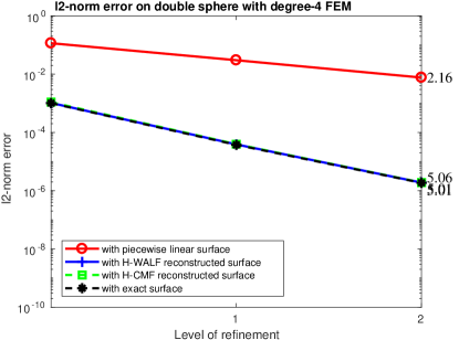
(a) Quartic FEM.

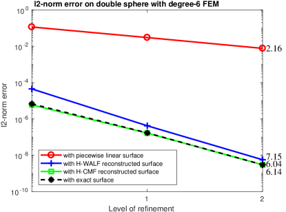
(b) Sextic FEM.

Figure 15: Convergence rates of FEM for solving Poisson equation with Dirichlet boundary conditions on double-sphere geometry.

For high-order FEM, the feature-aware parameterizations are important for both the surface and volume meshes. To demonstrate this, Figure 16 compares the solutions of quartic and sextic FEM for the same problem as above with four parameterization strategies:

• Non-FAP: neither the surface nor the volume elements used FAP;

• S-FAP: FAP is applied to surface elements but not to volume elements;

• V-FAP: FAP is applied to volume elements next to the boundary, but not to surface elements;

• SV-FAP: FAP is applied to both surface elements and volume elements next to the boundary.

It can be seen that V-FAP and SV-FAP improved accuracy significantly compared to Nno-FAP and S-FAP. This indicates that FAP for the volume elements has the most impact on FEM solutions. This impact is expected to be even greater if the boundary is concave or the degree is even higher. However, the FAP on the surface elements is also important, especially for degree-six FEM, when used in conjunction of FAP for the volume elements.

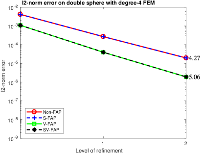
(a) Quartic FEM.

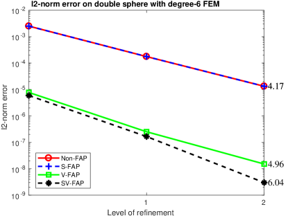
(b) Sextic FEM.

Figure 16: Demonstration of FAP for volume elements near boundaries in FEM with curved boundaries.

7 Conclusions

In this paper, we considered the problem of high-order reconstruction of a piecewise smooth surface from its surface triangulation. This is important for meshing, geometric modeling, finite element methods, etc. We introduced two Hermite-style surface reconstructions, called H-CMF and H-WALF, which extended the point-based CMF and WALF in [12] by taking into account the normals in addition to the points of the input mesh. In addition, we introduced an iterative feature-aware (IFA) parameterization for elements near sharp features and boundaries, which allows us to construct $G^{0}$ continuous parametric surfaces with guaranteed $(p+1)$st order accuracy for piecewise smooth surfaces. In addition, we also showed that with even-degree polynomials, the reconstructions can superconverge at about $(p+2)$nd order. We assessed the accuracy and stability of these techniques both through theoretical analysis and numerical experimentations. In terms of applications, we demonstrated that our high-order reconstructions enabled virtually indistinguishable results as using exact geometry for high-order FEM. This shows that our method provides a valuable tool for high-order FEM, either as an alternative to using exact CAD models when they are inconvenient to use (such as on supercomputers), or potentially as the only viable option if the CAD models are unavailable.

Our techniques only enforce $G^{0}$ continuity of the reconstructed surfaces, which is sufficient for most applications in terms of accuracy and stability of the numerical approximations, given that the local parameterizations are smooth. In comparison, some other techniques, such as NURBS, T-splines, moving least squares, etc., aim for $G^{1}$, $G^{2}$, or even $G^{\infty}$ continuities, which, however, have no direct correlation with the accuracy of numerical approximations. However, our proposed techniques are by no means replacements of traditional CAD techniques for all applications, as they can complement each other in different contexts. An important integration of the CAD models and the proposed Hermite-style reconstruction is the extraction of the surface normal and the feature curve tangents. Another extension of this work is to adapt the proposed techniques for high-order reconstructions of functions on surfaces, which are important for high-order data transfer across meshes in multiphysics simulations, as well as the high-order imposition of Neumann boundary conditions on curved geometries for some variants of finite element methods.

References

- [1] J. Donea, A. Huerta, J.-P. Ponthot, and A. Rodriguez-Ferran. Arbitrary Lagrangian-Eulerian methods. In E. Stein, R. de Borst, and T. J. Hughes, editors, Encyclopedia of Computational Mechanics, chapter 14. Wiley, 2004.
- [2] V. Dyedov, N. Ray, D. Einstein, X. Jiao, and T. Tautges. AHF: Array-based half-facet data structure for mixed-dimensional and non-manifold meshes. In J. Sarrate and M. Staten, editors, Proceedings of the 22nd International Meshing Roundtable, pages 445–464. Springer International Publishing, 2014.
- [3] G. Farin. Curves and Surfaces for Computer Aided Geometric Design. Academic Press, San Diego, 3rd edition, 1993.
- [4] S. Fleishman, D. Cohen-Or, and C. T. Silva. Robust moving least-squares fitting with sharp features. ACM Trans. Comput. Graph. (TOG), 24(3), 2005.
- [5] P. J. Frey and P. L. George. Mesh Generation: Application to finite elements. Hermes, 2000.
- [6] C. Geuzaine and J.-F. Remacle. Gmsh: a three-dimensional finite element mesh generator with built-in pre- and post-processing facilities. Int. J. Numer. Meth. Engrg., 79(11):1309–1331, 2009.
- [7] J. Goldfeather and V. Interrante. A novel cubic-order algorithm for approximating principal direction vectors. ACM Trans. Comput. Graph. (TOG), 23(1):45–63, 2004.
- [8] G. H. Golub and C. F. Van Loan. Matrix Computations. Johns Hopkins, 4th edition, 2013.
- [9] T. J. R. Hughes, J. A. Cottrell, and Y. Bazilevs. Isogeometric analysis: CAD, finite elements, NURBS, exact geometry, and mesh refinement. Comput. Meth. Appl. Mech. Engrg., 194:4135–4195, 2005.
- [10] X. Jiao and N. Bayyana. Identification of and discontinuities for surface meshes in CAD. Comput. Aid. Des., 40:160–175, 2008.
- [11] X. Jiao, A. Colombi, X. Ni, and J. Hart. Anisotropic mesh adaptation for evolving triangulated surfaces. Engrg. Comput., 26:363–376, 2010.
- [12] X. Jiao and D. Wang. Reconstructing high-order surfaces for meshing. Engrg. Comput., 28:361–373, 2012.
- [13] X. Jiao, D. Wang, and H. Zha. Simple and effective variational optimization of surface and volume triangulations. In Proceedings of 17th International Meshing Roundtable, pages 315–332, 2008.
- [14] X. Jiao and H. Zha. Consistent computation of first- and second-order differential quantities for surface meshes. In ACM Solid and Physical Modeling Symposium, pages 159–170. ACM, 2008.
- [15] D. Levin. The approximation power of moving least-squares. Math. Comput., 67:1517–1531, 1998.
- [16] F. Rapetti, A. Sommariva, and M. Vianello. On the generation of symmetric Lebesgue-like points in the triangle. J. Comput. Appl. Math., 236(18):4925–4932, 2012.
- [17] T. W. Sederberg, J. Zheng, A. Bakenov, and A. Nasri. T-splines and T-NURCCs. ACM Trans. Graph., 22(3):477–484, 2003.
- [18] A. van der Sluis. Condition numbers and equilibration of matrices. Numer. Math., 14:14–23, 1969.
- [19] A. Vlachos, J. Peters, C. Boyd, and J. L. Mitchell. Curved PN triangles. In Proc.of the 2001 Symposium on Interactive 3D graphics, pages 159–166, 2001.
- [20] D. Walton. A triangular G1 patch from boundary curves. Comput. Aid. Des., 28(2):113–123, 1996.
- [21] H. Wendland. Piecewise polynomial, positive definite and compactly supported radial functions of minimal degree. Adv. Comput. Math., 4(1):389–396, 1995.