Univariate tight wavelet frames of minimal support

Abstract

Wavelet frames for $L^{2}({\mathbb{R}})$ can be characterized by means of spectral techniques. This work uses spectral formulas to determine all the tight wavelet frames for $L^{2}(\mathbb{R})$ with a fixed finite number of generators of minimal support. The method associates wavelet frames of this type with certain inner operator-valued functions in Hardy spaces. The cases with one and two generators are completely solved.

Keywords: wavelet frames, Hardy spaces, inner functions

2010 MSC: 42C15, 30J05

1 Introduction

Let $T$ and $D$ be the translation and (dyadic) dilation unitary operators on $L^{2}(\mathbb{R})$ defined by

$$[Tf](x):=f(x-1)\,,\quad[Df](x):=2^{1/2}\,f(2x)\,,\quad(f\in L^{2}(\mathbb{R})).$$ (1)

Given a finite or countable subset $\Psi$ of $L^{2}(\mathbb{R})$, the (dyadic) wavelet system of $L^{2}(\mathbb{R})$ generated by $\Psi$ is of the form

$$X=X_{\Psi}:=\big{\{}\psi_{k,j}:=D^{k}T^{j}\psi:\psi\in\Psi,\,k,j\in\mathbb{Z}\big{\}}.$$ (2)

$X_{\Psi}$ is called a wavelet frame for $L^{2}(\mathbb{R})$ if there exist constants $A,B>0$ such that

$$A\,||f||^{2}\leq\sum_{\psi\in\Psi}\sum_{k,j\in\mathbb{Z}}|\langle f,\psi_{k,j}\rangle|^{2}\leq B\,||f||^{2},\quad(f\in L^{2}(\mathbb{R})).$$ (3)

If, in addition, $A=B$, it is said that $X_{\Psi}$ is a tight wavelet frame. The frame property (3) confers on $X_{\Psi}$ good properties for analysis and synthesis in $L^{2}(\mathbb{R})$.

A first paper [8] of this series characterizes the wavelet frames for $L^{2}({\mathbb{R}})$ by means of spectral techniques and presents the usual extension principles of the theory in terms of the periodized Fourier transform. Since the introduction of the extension principles [17, 18, 3, 5], the main part of the literature devoted to the construction of wavelet frames uses them looking for the corresponding framelet filter banks and paying attention to properties like vanishing moments, symmetry, number of generators, support, etc. In the univariate case see, e.g., [18, 2, 3, 4, 5, 22, 14, 10, 11, 1, 12]. The multivariate case in $L^{2}(\mathbb{R}^{d})$ is discussed in, e.g., [16, 21, 6, 15, 13].

In this work we use the spectral formulas obtained in [8] to calculate all the tight wavelet frames for $L^{2}(\mathbb{R})$ with a fixed finite number (say $r$) of generators of minimal support. Like in [7], Hardy classes of vector-valued functions and operator-valued inner functions play a central role. We solve explicitly the cases $r=1$ and $r=2$. To our knowledge, there are no papers in the literature studying this problem. In the context of extension principles, the tight framelet filter banks with $r=1$ are characterized in [12, Theorem 7]. For $r=2$, Theorem 4.2 in [10] gives the tight framelet filter banks with complex symmetry and other partial results can be found in, e.g., [18, 2, 3, 5, 22]. In particular, the case with B-splines as refinable functions has been extensively studied; see, e.g., [6, Section 4.4] for details.

Section 2 below introduces the terminology and notation used in spectral methods necessary along the paper. We also recall the spectral characterization of tight wavelet frames for $L^{2}(\mathbb{R})$ given in [8, Corollary 3.6].

Section 3 shows how [8, Corollary 3.6] permits us to determine all the tight wavelet frames for $L^{2}(\mathbb{R})$ with a fixed number of generators of minimal support. Like in [7], Hardy classes [19, 20, 9] play a central role here. In particular, operator-valued functions called rigid Taylor operator functions by Halmos [9] and $M^{+}$-inner functions by Rosenblum and Rovnyak [19]. See section 3.1 below for details. Roughly speaking, Halmos lemma 3.3, Rovnyak lemma 3.4 and proposition 3.5 imply the following result:

Let $X_{\Psi}$ be a wavelet system of the form (2), with cardinal of $\Psi$ finite, say $r$, and such that the support of each $\psi\in\Psi$ is included in the interval $[0,1]$. Then, $X_{\Psi}$ is a tight wavelet frame for $L^{2}(\mathbb{R})$ if and only if $\Psi$ is associated with an $M^{+}$-inner $(r\times r)$-matrix function $A^{+}(\omega)$ satisfying certain properties.

This result comes from a particular choice of orthonormal bases $\big{\{}L_{i}^{(n)}\big{\}}$ and $\big{\{}K_{s,j}^{(m)}\big{\}}$ in the spectral method, the Haar orthonormal bases given in the appendix, and the corresponding distribution of indices in the set of equations (12) –see proposition 3.2, in particular, table 1–.

We discuss the cases $r=1$ and $r=2$ in sections 3.2 and 3.3, respectively. For $r=1$ the solution is given in corollary 3.6:

The only function $\psi\in L^{2}[0,1]$ such that the wavelet system $X_{\Psi}$ of the form (2) generated by $\Psi=\{\psi\}$ is a tight frame for $L^{2}(\mathbb{R})$, with frame bound $B$, is proportional to the Haar wavelet:

$$\psi=\beta\,[\chi_{[0,1/2)}-\chi_{[1/2,1)}],$$

where $\beta\in\mathbb{C}$ and $|\beta|^{2}=B$. It is associated with the constant $M^{+}$-inner scalar function

$$A^{+}:\partial\mathbb{D}\to\mathbb{C}:\omega\mapsto\beta/|\beta|\,.$$

This result invalidates theorem 5 in [7]. See remark 3.7 for more details.

For $r=2$, i.e., $\Psi=\{\psi_{1},\psi_{2}\}\subset L^{2}[0,1]$, the $M^{+}$-inner $(2\times 2)$-matrix functions $A^{+}(\omega)$ of interest appear in proposition 3.10 and the final solution is given in propositions 3.11 and 3.12:

There are five types of families of $M^{+}$-inner ($2\times 2$)-matrix functions

$$A^{+}(\omega)=\left(\begin{array}[]{cc}{\mathfrak{a}}^{(0)}_{1}(\omega)&{\mathfrak{a}}^{(1)}_{1}(\omega)\\ {\mathfrak{a}}^{(0)}_{2}(\omega)&{\mathfrak{a}}^{(1)}_{2}(\omega)\end{array}\right)=\left(\begin{array}[]{cc}{\mathfrak{a}}^{(0)}(\omega)&{\mathfrak{a}}^{(1)}(\omega)\end{array}\right)\,,\quad\text{ where }{\mathfrak{a}}^{(0)},{\mathfrak{a}}^{(1)}\in H^{+}_{\mathbb{C}^{2}}\,,$$

leading to tight wavelet frames $X_{\Psi}$ of the form (2) generated by $\Psi$. They are as follows:

• Given $u_{0}\in\mathbb{C}^{2}$, such that $||u_{0}||_{\mathbb{C}^{2}}=1$,

  $$\left\{\begin{array}[]{l}\displaystyle{\mathfrak{a}}^{(0)}(\omega)=u_{0}\,,\\ {\mathfrak{a}}^{(1)}(\omega)=0\,.\end{array}\right.$$

• Given an orthonormal basis $\{u_{0},u_{1}\}$ of $\mathbb{C}^{2}$,

  $$\left\{\begin{array}[]{l}\displaystyle{\mathfrak{a}}^{(0)}(\omega)=\omega\,u_{0}\,,\\ {\mathfrak{a}}^{(1)}(\omega)=u_{1}\,.\end{array}\right.$$

• Given an orthonormal basis $\{u_{0},u_{1}\}$ of $\mathbb{C}^{2}$, $0<\rho<1$ and $\theta\in\mathbb{R}$,

  $$\left\{\begin{array}[]{l}\displaystyle{\mathfrak{a}}^{(0)}(\omega)=\rho u_{0}+\omega(1-\rho^{2})^{1/2}u_{1}\,,\\ \displaystyle{\mathfrak{a}}^{(1)}(\omega)=e^{i\theta}[(1-\rho^{2})^{1/2}u_{0}-\omega\,\rho u_{1}]\,.\end{array}\right.$$

• Given an orthonormal basis $\{u_{0},u_{1}\}$ of $\mathbb{C}^{2}$, $0<\rho<1$ and $\theta\in\mathbb{R}$,

  $$\left\{\begin{array}[]{l}\displaystyle{\mathfrak{a}}^{(0)}(\omega)=\big{(}\rho+(1-\rho^{2})e^{i\theta}\sum_{k=1}^{\infty}\omega^{k}\,\big{(}-\rho\,e^{i\theta}\big{)}^{k-1}\big{)}\,u_{0}\,,\\ \displaystyle{\mathfrak{a}}^{(1)}(\omega)=u_{1}\,.\end{array}\right.$$

• Given $0<|\rho_{0}|<1$, choose three unitary vectors $u_{0}$, $u_{1}$ and $v$ in $\mathbb{C}^{2}$ such that (71) is satisfied. Then, $|\rho_{1}|$ and $|\tau_{0}|$ are given by (77). Once the free arguments for $\rho_{0}$, $\rho_{1}$ and $\tau_{0}$ have been selected, say $\theta_{\rho_{0}}$, $\theta_{\rho_{1}}$ and $\theta_{\tau_{0}}$, the value of $r$ is determined by (74) and the value of $\tau_{1}$ is given by (77). Then,

  $$\left\{\begin{array}[]{l}\displaystyle{\mathfrak{a}}^{(0)}(\omega)=\rho_{0}u_{0}+\rho_{1}v\sum_{k=1}^{\infty}\omega^{k}\,r^{k-1}\,,\\ \displaystyle{\mathfrak{a}}^{(1)}(\omega)=\tau_{0}u_{1}+\tau_{1}v\sum_{k=1}^{\infty}\omega^{k}\,r^{k-1}\,.\end{array}\right.$$

In order to obtain $\psi_{1}$ and $\psi_{2}$ from the function $A^{+}(\omega)$ one must proceed in the following way. Since $\text{supp}\,\psi_{j}\subseteq[0,1]$, ($j=1,2$), their expansions (6) read

$$\psi_{j}=\sum_{i\in\mathbb{N}\cup\{0\}}[\hat{\psi}_{j}]_{i}^{(0)}L_{i}^{(0)}\,,\quad(j=1,2)\,.$$

Let us write

$$\Psi_{i}:=\left(\begin{array}[]{c}[\hat{\psi}_{1}]_{i}^{(0)}\cr[\hat{\psi}_{2}]_{i}^{(0)}\end{array}\right)\in\mathbb{C}^{2}\,,\quad(i\in\mathbb{N}\cup\{0\})\,.$$

Then, for a frame bound $B>0$,

$$\begin{array}[]{l}\displaystyle\sum_{k=0}^{\infty}\omega^{k}\,\Psi_{2^{k}}=B_{0}\,{\mathfrak{a}}^{(0)}(\omega)\,,\\[8.61108pt] \displaystyle\sum_{k=0}^{\infty}\omega^{k}\,\Psi_{2^{p+k+1}+l}=C_{l}\,{\mathfrak{a}}^{(1)}(\omega)\,,\quad(l\geq 1,\,l=2^{p}+\sum_{t=0}^{p-1}l_{t}2^{t})\,,\end{array}$$

where $B_{0}\in\mathbb{C}$ is such that $|B_{0}|^{2}=B$ and the sequence $\{C_{l}\}_{l\in\mathbb{N}}\subset\mathbb{C}$ is given by (44)–(46) and (30).

Clearly, for type 1 functions $A^{+}(\omega)$, both functions $\psi_{1}$ and $\psi_{2}$ are proportional to the Haar wavelet. For types 2–5 functions $A^{+}(\omega)$, some examples of real functions $\psi_{1}$ and $\psi_{2}$ are shown in figures 1–4. As it can be seen in figures 2 and 3, type 3 functions $A^{+}(\omega)$ lead to the reflected version of functions $\psi_{1}$ and $\psi_{2}$ obtained from type 4 functions $A^{+}(\omega)$ with the same parameters.

Given an $M^{+}$-inner ($2\times 2$)-matrix function $A^{+}(\omega)$ of type 2–5, also $B^{+}(\omega)=A^{+}(\omega)\cdot U$ is an $M^{+}$-inner ($2\times 2$)-matrix function of type 2–5, for every constant unitary ($2\times 2$)-matrix $U$. This relationship establishes connections between $M^{+}$-inner ($2\times 2$)-matrix functions of types 2 and 3 on the one hand and $M^{+}$-inner ($2\times 2$)-matrix functions of types 4 and 5 on the other hand. See proposition 3.13 and comments that follow it. Thus, starting from a simple tight wavelet frame of type 2, one can obtain a frame of type 3 by means of a unitary matrix $U$, to get a frame of type 4 by reflection and, finally, to reach a frame of type 5 using again a unitary matrix $U^{\prime}$.

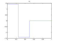
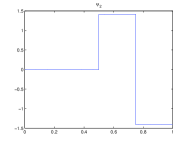
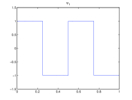
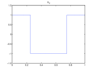
(a) Parameters: $u_{0}=(1,0),\,u_{1}=(0,1)$,		(b) Parameters: $u_{0}=(1,1)/\sqrt{2},\,u_{1}=(1,-1)/\sqrt{2}$,
$B_{0}=1$ and $\text{arg}(C_{1})=0$.		$B_{0}=1$ and $\text{arg}(C_{1})=0$.

Figure 1: Case $r=2$. Examples of real functions $\psi_{1}$ and $\psi_{2}$ of type 2.

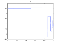
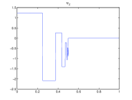
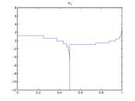
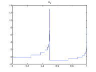
(a) Parameters: ${\mathfrak{u}}_{0}=(1,0),\,{\mathfrak{u}}_{1}=(0,1)$,		(b) Parameters: ${\mathfrak{u}}_{0}=(1,1)/\sqrt{2},\,{\mathfrak{u}}_{1}=(1,-1)/\sqrt{2}$,
$\rho=1/2$, $B_{0}=1$, $\text{arg}(C_{1})=0$ and $\theta=0$.		$\rho=3/4$, $B_{0}=1$, $\text{arg}(C_{1})=0$ and $\theta=\pi$.

Figure 2: Case $r=2$. Examples of real functions $\psi_{1}$ and $\psi_{2}$ of type 3.

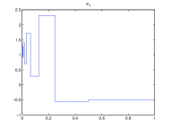
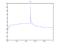
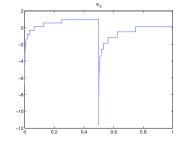
(a) Parameters: ${\mathfrak{u}}_{0}=(1,0),\,{\mathfrak{u}}_{1}=(0,1)$,		(b) Parameters: ${\mathfrak{u}}_{0}=(1,1)/\sqrt{2},\,{\mathfrak{u}}_{1}=(1,-1)/\sqrt{2}$,
$\rho=1/2$, $B_{0}=1$, $\text{arg}(C_{1})=0$ and $\theta=0$.		$\rho=3/4$, $B_{0}=1$, $\text{arg}(C_{1})=0$ and $\theta=\pi$.

Figure 3: Case $r=2$. Examples of real functions $\psi_{1}$ and $\psi_{2}$ of type 4.

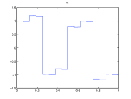
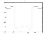
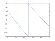
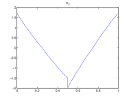
(a) Parameters: $\rho_{0}=0.1$, $u_{0}=(1,0)$, $v=(1,1)/\sqrt{2}$,		(d) Parameters: $\rho_{0}=-1/2$, $u_{0}=(1,0)$, $v=(1,1)/\sqrt{2}$,
$\text{arg}(\rho_{1})=\text{arg}(\tau_{0})=0$, $B_{0}=1$ and $\text{arg}(C_{1})=0$.		$\text{arg}(\rho_{1})=\text{arg}(\tau_{0})=0$, $B_{0}=1$ and $\text{arg}(C_{1})=0$.
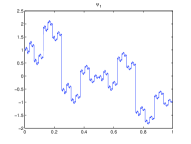
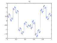
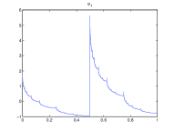
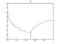
(b) Parameters: $\rho_{0}=1/2$, $u_{0}=(1,0)$, $v=(1,1)/\sqrt{2}$,		(e) Parameters: $\rho_{0}=-0.6$, $u_{0}=(1,1)/\sqrt{2}$, $v=(1,2)/\sqrt{5}$,
$\text{arg}(\rho_{1})=\text{arg}(\tau_{0})=0$, $B_{0}=1$ and $\text{arg}(C_{1})=0$.		$\text{arg}(\rho_{1})=\text{arg}(\tau_{0})=0$, $B_{0}=1$ and $\text{arg}(C_{1})=0$.
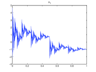
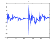
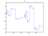
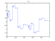
(c) Parameters: $\rho_{0}=0.9$, $u_{0}=(1,0)$, $v=(1,1)/\sqrt{2}$,		(f) Parameters: $\rho_{0}=1/2$, $u_{0}=(1,1)/\sqrt{2}$, $v=(1,2)/\sqrt{5}$,
$\text{arg}(\rho_{1})=\text{arg}(\tau_{0})=0$, $B_{0}=1$ and $\text{arg}(C_{1})=0$.		$\text{arg}(\rho_{1})=\text{arg}(\tau_{0})=0$, $B_{0}=1$ and $\text{arg}(C_{1})=0$.

Figure 4: Case $r=2$. Examples of real functions $\psi_{1}$ and $\psi_{2}$ of type 5.

2 Preliminaries

The spectral techniques for univariate wavelet frames developed in [8] are based on suitable spectral representations of the translation and dilation operators $T$ and $D$ given in (1). These representations are built in terms of an orthonormal basis (shortly, ONB) $\{L_{i}^{(0)}(x)\}_{i\in\mathbb{I}}$ of $L^{2}[0,1)$ and ONBs $\{K_{\pm,j}^{(0)}(x)\}_{j\in\mathbb{J}}$ of $L^{2}[\pm 1,\pm 2)$, where $\mathbb{I}$, $\mathbb{J}$ are denumerable sets of indices (usually, $\mathbb{N}$, $\mathbb{N}\cup\{0\}$ or $\mathbb{Z}$). Obviously, the families

$$\big{\{}L_{i}^{(n)}(x):=[T^{n}L_{i}^{(0)}](x)=L_{i}^{(0)}(x-n)\big{\}}_{i\in\mathbb{I},n\in\mathbb{Z}},$$ (4)

$$\big{\{}K_{s,j}^{(m)}(x):=[D^{m}K_{s,j}^{(0)}](x)=2^{m/2}K_{s,j}^{(0)}(2^{m}x)\big{\}}_{j\in\mathbb{J},m\in\mathbb{Z},s=\pm}$$ (5)

are ONBs of $L^{2}(\mathbb{R})$ and, for each $f\in L^{2}(\mathbb{R})$, one has (in $L^{2}$-sense)

$$f=\sum_{i,n}\hat{f}^{(n)}_{i}L_{i}^{(n)},\text{ with }\hat{f}^{(n)}_{i}:=\langle f,L_{i}^{(n)}\rangle_{L^{2}(\mathbb{R})}\,,$$ (6)

$$f=\sum_{s,j,m}\tilde{f}^{(m)}_{s,j}K_{s,j}^{(m)},\text{ with }\tilde{f}^{(m)}_{s,j}:=\langle f,K_{s,j}^{(m)}\rangle_{L^{2}(\mathbb{R})}\,.$$ (7)

The change of representation between both expansions (6) and (7) is governed by a matrix $\big{(}\alpha_{i,n}^{s,j,m}\big{)}$, where

$$\alpha_{i,n}^{s,j,m}:=\langle L_{i}^{(n)},K_{s,j}^{(m)}\rangle_{L^{2}(\mathbb{R})}\,.$$ (8)

In what follows, fixed ONBs $\{L_{i}^{(n)}(x)\}_{i\in\mathbb{I},n\in\mathbb{Z}}$ and $\{K_{s,j}^{(m)}(x)\}_{j\in\mathbb{J},m\in\mathbb{Z},s=\pm}$ of $L^{2}(\mathbb{R})$ as above, for each $f\in L^{2}(\mathbb{R})$ we shall write

$$f=\big{\{}\hat{f}_{i}^{(n)}\big{\}}=\big{\{}\tilde{f}_{s,j}^{(m)}\big{\}}$$

and we shall also use the notation

$$\hat{f}_{i}(\omega):=\sum_{n\in\mathbb{Z}}\omega^{n}\,\hat{f}_{i}^{(n)}\quad\text{and}\quad\tilde{f}_{s,j}(\omega):=\sum_{m\in\mathbb{Z}}\omega^{m}\,\tilde{f}_{s,j}^{(m)}\,,\quad(f\in L^{2}(\mathbb{R});i\in\mathbb{I};s=\pm,j\in\mathbb{J})\,.$$

Corollary 3.6 in [8] gives a useful description of tight wavelet frames for $L^{2}(\mathbb{R})$:

A wavelet system $X_{\Psi}$ of the form (2) and such that

$$\sup_{\psi\in\Psi}||\psi||_{L^{2}(\mathbb{R})}=M<\infty$$ (9)

is a tight frame for $L^{2}(\mathbb{R})$, with frame bound $B$, if and only if

$$\sum_{\stackrel{{\scriptstyle i,n}}{{i^{\prime},n^{\prime}}}}\big{(}{\sum_{k,j\in\mathbb{Z}}}^{u}\,\overline{\alpha_{i,n+j}^{s,l,k}}\,\alpha_{i^{\prime},n^{\prime}+j}^{s^{\prime},l^{\prime},k+\sigma}\big{)}\big{(}{\sum_{\psi\in\Psi}}^{u}\,\overline{\hat{\psi}_{i}^{(n)}}\,\hat{\psi}_{i^{\prime}}^{(n^{\prime})}\big{)}=B\,\delta_{s,s^{\prime}}\delta_{l-l^{\prime}}\delta_{\sigma}\,,\quad(s,s^{\prime}=\pm,\,l,l^{\prime}\in\mathbb{J},\,\sigma\in\mathbb{Z})\,.$$ (10)

Here, $\delta$ denotes the Dirac $\delta$-function, the superindex ’u’ added to the sum symbols $\sum$ reflects the unconditional convergence of the series (see [8, Lemma 3.4] and comments that follow it), and the components $\big{\{}\hat{\psi}_{i}^{(n)}\big{\}}$ of each $\psi\in\Psi$ and the $\alpha_{i,n}^{s,j,m}$’s are related with the spectral representations of section 2 (see equations (6) and (8)).

3 Tight wavelet frames of minimal support

In this section, Corollary 3.6 in [8] is used to determine all the tight wavelet frames for $L^{2}(\mathbb{R})$ of the form (2), with cardinal of $\Psi$ finite and such that the support of each $\psi\in\Psi$, $\text{supp}\,\psi$, is included in the interval $[0,1]$. Note that, since the cardinal of $\Psi$ is finite, condition (9) is trivially satisfied.

Due to the structure of the ONB $\big{\{}L_{i}^{(j)}\big{\}}$, defined by (4), the fact that $\text{supp}\,\psi\subseteq[0,1]$, ($\psi\in\Psi$), implies that their expansions (6) read

$$\psi=\sum_{i\in\mathbb{I}}\hat{\psi}_{i}^{(0)}L_{i}^{(0)}\,,\quad(\psi\in\Psi)\,,$$

since $\hat{\psi}_{i}^{(n)}=0$ for $n\neq 0$. Thus, for non-zero summands in the left hand side of (10) it must be $n=n^{\prime}=0$, so that

$$\sum_{\stackrel{{\scriptstyle i,n}}{{i^{\prime},n^{\prime}}}}\big{(}{\sum_{k,j\in\mathbb{Z}}}^{u}\,\overline{\alpha_{i,n+j}^{s,l,k}}\,\alpha_{i^{\prime},n^{\prime}+j}^{s^{\prime},l^{\prime},k+\sigma}\big{)}\big{(}{\sum_{\psi\in\Psi}}^{u}\,\overline{\hat{\psi}_{i}^{(n)}}\,\hat{\psi}_{i^{\prime}}^{(n^{\prime})}\big{)}=\sum_{{i,i^{\prime}}}\big{(}{\sum_{k,j\in\mathbb{Z}}}^{u}\,\overline{\alpha_{i,j}^{s,l,k}}\,\alpha_{i^{\prime},j}^{s^{\prime},l^{\prime},k+\sigma}\big{)}\big{(}{\sum_{\psi\in\Psi}}^{u}\,\overline{\hat{\psi}_{i}^{(0)}}\,\hat{\psi}_{i^{\prime}}^{(0)}\big{)}\,.$$ (11)

Now, being finite the cardinal of $\Psi$, according to [8, Lemma 3.4] and the comments that follow it, the unconditional sums in (11) may be calculated, for example, in the following way:

$$\sum_{{i,i^{\prime}}}\big{(}{\sum_{k,j\in\mathbb{Z}}}^{u}\,\overline{\alpha_{i,j}^{s,l,k}}\,\alpha_{i^{\prime},j}^{s^{\prime},l^{\prime},k+\sigma}\big{)}\big{(}{\sum_{\psi\in\Psi}}^{u}\,\overline{\hat{\psi}_{i}^{(0)}}\,\hat{\psi}_{i^{\prime}}^{(0)}\big{)}=\lim_{a\to\infty}\sum_{i,i^{\prime}}\big{[}\sum_{k=-a}^{a}\sum_{j=-2^{a}}^{2^{a}}\overline{\alpha_{i,j}^{s,l,k}}\alpha_{i^{\prime},j}^{s^{\prime},l^{\prime},k+\sigma}\big{]}\big{[}\sum_{\psi\in\Psi}\overline{\hat{\psi}_{i}^{(0)}}\hat{\psi}_{i^{\prime}}^{(0)}\big{]}\,.$$

Then, in this particular case, Corollary 3.6 in [8] can be rewritten as follows:

Proposition 3.1

Let $X$ be a wavelet system in $L^{2}(\mathbb{R})$ of the form (2), where $\Psi$ has finite cardinal and $\text{supp}\,\psi\subseteq[0,1]$ for every $\psi\in\Psi$. Then, $X$ is a tight frame for $L^{2}(\mathbb{R})$, with frame bound $B$, if and only if

$$\lim_{a\to\infty}\sum_{i,i^{\prime}\in\mathbb{I}}\big{[}\sum_{k=-a}^{a}\sum_{j=-2^{a}}^{2^{a}}\overline{\alpha_{i,j}^{s,l,k}}\alpha_{i^{\prime},j}^{s^{\prime},l^{\prime},k+\sigma}\big{]}\big{[}\sum_{\psi\in\Psi}\overline{\hat{\psi}_{i}^{(0)}}\hat{\psi}_{i^{\prime}}^{(0)}\big{]}=B\,\delta_{s,s^{\prime}}\delta_{l-l^{\prime}}\delta_{\sigma},\quad(s,s^{\prime}=\pm,\,l,l^{\prime}\in\mathbb{J},\,\sigma\in\mathbb{Z}).$$ (12)

From now on, we consider the Haar orthonormal bases $\big{\{}L_{i}^{(j)}\big{\}}$ and $\big{\{}K_{s,l}^{(k)}\big{\}}$ and the corresponding matrix $\big{(}\alpha_{i,j}^{s,l,k}\big{)}$ given in the appendix. This choice leads to the following result, which we write in vectorial form:

Proposition 3.2

Let $\big{\{}L_{i}^{(0)}\big{\}}_{i\in\mathbb{N}\cup\{0\}}$ be the Haar orthonormal basis of $L^{2}[0,1]$ given in (81). Let $r\in\mathbb{N}$ and

$$\Psi=\{\psi_{1},\psi_{2},\ldots,\psi_{r}\}\subset L^{2}[0,1]\,,$$

where $\psi_{j}=\sum_{i}[\hat{\psi}_{j}]_{i}^{(0)}L_{i}^{(0)}$, ($j=1,\ldots,r$). Let us put

$$\Psi_{i}:=\left(\begin{array}[]{c}[\hat{\psi}_{1}]_{i}^{(0)}\cr[\hat{\psi}_{2}]_{i}^{(0)}\cr\vdots\cr[\hat{\psi}_{r}]_{i}^{(0)}\end{array}\right)\in\mathbb{C}^{r},\quad(i\in\mathbb{N}\cup\{0\}).$$

Then, the wavelet system $X$ of the form (2) generated by $\Psi$ is a tight frame for $L^{2}(\mathbb{R})$, with frame bound $B$, if and only if the following conditions are satisfied:

1. $\Psi_{0}=(0,0,\ldots,0)\in\mathbb{C}^{r}$.

2. $$\sum_{k=\sup\{1,1-\sigma\}}^{\infty}\langle\Psi_{2^{k-1+\sigma}},\Psi_{2^{k-1}}\rangle_{\mathbb{C}^{r}}=B\,\delta_{\sigma},\quad(\sigma\in\mathbb{Z}).$$ (13)

3. For $l\geq 1$, $l=2^{p}+\sum_{t=0}^{p-1}l_{t}2^{t}$, ($p\geq 0$),

   $$\sum_{k=-p}^{0}||\Psi_{2^{p+k}+\sum_{t=0}^{p+k-1}l_{t}2^{t}}||^{2}_{\mathbb{C}^{r}}+\sum_{k=1}^{\infty}||\Psi_{2^{p+k}+l}||^{2}_{\mathbb{C}^{r}}=B,$$ (14)

   $$\sum_{k=\sup\{1,1-\sigma\}}^{\infty}\langle\Psi_{2^{p+k+\sigma}+l},\Psi_{2^{p+k}+l}\rangle_{\mathbb{C}^{r}}=0,\quad(\sigma\in\mathbb{Z}\backslash\{0\}),$$ (15)

   $$\sum_{k=\sup\{1,1-\sigma\}}^{\infty}\langle\Psi_{2^{p+k+\sigma}+l},\Psi_{2^{k-1}}\rangle_{\mathbb{C}^{r}}=0,\quad(\sigma\in\mathbb{Z}).$$ (16)

4. For $l,l^{\prime}\geq 1$, $l\neq l^{\prime}$, $l=2^{p}+\sum_{t=0}^{p-1}l_{t}2^{t}$, $l^{\prime}=2^{p^{\prime}}+\sum_{t=0}^{p^{\prime}-1}l^{\prime}_{t}2^{t}$, ($p,p^{\prime}\geq 0$),

   $$\begin{array}[]{c}\displaystyle\sum_{k=\sup\{-p,-p^{\prime}\}}^{0}\delta_{(\sum_{t=0}^{-k}l_{p+k+t}2^{t})-(\sum_{t=0}^{-k}l^{\prime}_{p^{\prime}+k+t}2^{t})}\,\langle\Psi_{2^{p^{\prime}+k}+\sum_{t=0}^{p^{\prime}+k-1}l^{\prime}_{t}2^{t}},\Psi_{2^{p+k}+\sum_{t=0}^{p+k-1}l_{t}2^{t}}\rangle_{\mathbb{C}^{r}}+\\ \displaystyle+\sum_{k=1}^{\infty}\langle\Psi_{2^{p^{\prime}+k}+l^{\prime}},\Psi_{2^{p+k}+l}\rangle_{\mathbb{C}^{r}}=0,\end{array}$$ (17)

   $$\sum_{k=\sup\{1,1-\sigma\}}^{\infty}\langle\Psi_{2^{p^{\prime}+k+\sigma}+l^{\prime}},\Psi_{2^{p+k}+l}\rangle_{\mathbb{C}^{r}}=0,\quad(\sigma\in\mathbb{Z}\backslash\{0\}).$$ (18)

Proof.

In order to avoid additional indices along the proof, we work with generic $\psi\in\Psi$ and not with $\psi_{1},\ldots,\psi_{r}$. Consider the Haar orthonormal bases $\big{\{}L_{i}^{(j)}\big{\}}$ and $\big{\{}K_{s,l}^{(k)}\big{\}}$ and the corresponding matrix $\big{(}\alpha_{i,j}^{s,l,k}\big{)}$ given in the appendix. For $s=s^{\prime}=+$, $l=l^{\prime}=0$ and $\sigma=0$ in (12) one obtains

$$\displaystyle\lim_{a\to\infty}\sum_{i,i^{\prime}}\big{[}\sum_{k=-a}^{a}\sum_{j=-2^{a}}^{2^{a}}\overline{\alpha_{i,j}^{s,l,k}}\alpha_{i^{\prime},j}^{s^{\prime},l^{\prime},k+\sigma}\big{]}\big{[}\sum_{\psi}\overline{\hat{\psi}_{i}^{(0)}}\hat{\psi}_{i^{\prime}}^{(0)}\big{]}=$$

$$\displaystyle=\lim_{a\to\infty}\big{(}a+1+\sum_{k=1}^{a}2^{-k}\big{)}\big{[}\sum_{\psi}|\hat{\psi}_{0}^{(0)}|^{2}\big{]}+\sum_{r=0}^{\infty}\big{[}\sum_{\psi}|\hat{\psi}_{2^{r}}^{(0)}|^{2}\big{]}.$$

The last expression can be equal to $B$ if and only if $\hat{\psi}_{0}^{(0)}=\int\psi=0$ for every $\psi\in\Psi$, which is condition 1 in the statement, and $\sum_{r=0}^{\infty}\big{[}\sum_{\psi}|\hat{\psi}_{2^{r}}^{(0)}|^{2}\big{]}=B$, the condition (13) for $\sigma=0$ in the statement. Assuming then that $\hat{\psi}_{0}^{(0)}=0$ for every $\psi\in\Psi$, straightforward calculations with the $\alpha_{i,j}^{s,l,k}$’s lead to the fact that the conditions in (12), for $s=s^{\prime}=+$, are related with table 1.

$s=s^{\prime}=+$	$2^{0}$	$2^{1}$	$2^{2}$	$2^{3}$	$\cdots$
$\mathbf{l,l^{\prime}=0}$ (0)	$k,k+\sigma=1$ $j=0$ $i,i^{\prime}=2^{0}$	$k,k+\sigma=2$ $j=0$ $i,i^{\prime}=2^{1}$	$k,k+\sigma=3$ $j=0$ $i,i^{\prime}=2^{2}$	$k,k+\sigma=4$ $j=0$ $i,i^{\prime}=2^{3}$	$\cdots$
$\mathbf{l,l^{\prime}=1}$ (1)	$\mathbf{k,k+\sigma=0}$ $\mathbf{j=1}$ $\mathbf{i,i^{\prime}=2^{0}}$	$k,k+\sigma=1$ $j=0$ $i,i^{\prime}=2^{1}+1$	$k,k+\sigma=2$ $j=0$ $i,i^{\prime}=2^{2}+1$	$k,k+\sigma=3$ $j=0$ $i,i^{\prime}=2^{3}+1$	$\cdots$
$\mathbf{l,l^{\prime}=2}$ (10)	$k,k+\sigma=-1$ $j=2$ $i,i^{\prime}=2^{0}$	$\mathbf{k,k+\sigma=0}$ $\mathbf{j=1}$ $\mathbf{i,i^{\prime}=2^{1}}$	$k,k+\sigma=1$ $j=0$ $i,i^{\prime}=2^{2}+2$	$k,k+\sigma=2$ $j=0$ $i,i^{\prime}=2^{3}+2$	$\cdots$
$\mathbf{l,l^{\prime}=3}$ (11)	$k,k+\sigma=-1$ $j=3$ $i,i^{\prime}=2^{0}$	$\mathbf{k,k+\sigma=0}$ $\mathbf{j=1}$ $\mathbf{i,i^{\prime}=2^{1}+1}$	$k,k+\sigma=1$ $j=0$ $i,i^{\prime}=2^{2}+3$	$k,k+\sigma=2$ $j=0$ $i,i^{\prime}=2^{3}+3$	$\cdots$
$\mathbf{l,l^{\prime}=4}$ (100)	$k,k+\sigma=-2$ $j=4$ $i,i^{\prime}=2^{0}$	$k,k+\sigma=-1$ $j=2$ $i,i^{\prime}=2^{1}$	$\mathbf{k,k+\sigma=0}$ $\mathbf{j=1}$ $\mathbf{i,i^{\prime}=2^{2}}$	$k,k+\sigma=1$ $j=0$ $i,i^{\prime}=2^{3}+4$	$\cdots$
$\mathbf{l,l^{\prime}=5}$ (101)	$k,k+\sigma=-2$ $j=5$ $i,i^{\prime}=2^{0}$	$k,k+\sigma=-1$ $j=2$ $i,i^{\prime}=2^{1}+1$	$\mathbf{k,k+\sigma=0}$ $\mathbf{j=1}$ $\mathbf{i,i^{\prime}=2^{2}+1}$	$k,k+\sigma=1$ $j=0$ $i,i^{\prime}=2^{3}+5$	$\cdots$
$\mathbf{l,l^{\prime}=6}$ (110)	$k,k+\sigma=-2$ $j=6$ $i,i^{\prime}=2^{0}$	$k,k+\sigma=-1$ $j=3$ $i,i^{\prime}=2^{1}$	$\mathbf{k,k+\sigma=0}$ $\mathbf{j=1}$ $\mathbf{i,i^{\prime}=2^{2}+2}$	$k,k+\sigma=1$ $j=0$ $i,i^{\prime}=2^{3}+6$	$\cdots$
$\mathbf{l,l^{\prime}=7}$ (111)	$k,k+\sigma=-2$ $j=7$ $i,i^{\prime}=2^{0}$	$k,k+\sigma=-1$ $j=3$ $i,i^{\prime}=2^{1}+1$	$\mathbf{k,k+\sigma=0}$ $\mathbf{j=1}$ $\mathbf{i,i^{\prime}=2^{2}+3}$	$k,k+\sigma=1$ $j=0$ $i,i^{\prime}=2^{3}+7$	$\cdots$
$\vdots$	$\vdots$	$\vdots$	$\vdots$	$\vdots$	$\ddots$

$s=s^{\prime}=+$	$2^{r},\,(0\leq r<p)$	$2^{p}$	$2^{r},\,(r>p)$
$\mathbf{l,l^{\prime}>0}$ ($l,l^{\prime}=2^{p}+\sum_{t=0}^{p-1}l_{t}2^{t}$)	$k,k+\sigma=r-p$ $j=\sum_{t=0}^{p-r}l_{r+t}2^{t}$ $i,i^{\prime}=2^{r}+\sum_{t=0}^{r-1}l_{t}2^{t}$	$\mathbf{k,k+\sigma=0}$ $\mathbf{j=1}$ $\mathbf{i,i^{\prime}=l,l^{\prime}}$	$k,k+\sigma=r-p$ $j=0$ $i,i^{\prime}=2^{r}+l$

Table 1: Distribution of indices for $s=s^{\prime}=+$ in the set of equations (12) using the Haar orthonormal bases $\big{\{}L_{i}^{(j)}\big{\}}$ and $\big{\{}K_{s,l}^{(k)}\big{\}}$ and the corresponding matrix $\big{(}\alpha_{i,j}^{s,l,k}\big{)}$ given in the appendix. See the proof of proposition 3.2 for details.

To obtain the conditions in (12), for $s=s^{\prime}=+$, table 1 is used as follows: Choose the values of $l$ and $l^{\prime}$, and consider the corresponding files in the table. Choose the value of $\sigma$. In each entry of the table, the indices $k$ and $i$ are associated with $l$, and the indices $k+\sigma$ and $i^{\prime}$ are associated with $l^{\prime}$. One must pair the columns with the same $k$ and $j$ in both files, multiply $\overline{\hat{\psi}_{i}^{(0)}}$ by $\hat{\psi}_{i^{\prime}}^{(0)}$ for the indices $i$, $i^{\prime}$ selected in the paired columns, sum over $\psi\in\Psi$ and, finally, sum over all the paired columns. For example, for $l=l^{\prime}=0$ and $\sigma=0$ we arrive to the already known equation

$$\sum_{k=1}^{\infty}\big{[}\sum_{\psi}|\hat{\psi}_{2^{k-1}}^{(0)}|^{2}\big{]}=B,$$

the condition (13) for $\sigma=0$ in the statement. For $l=l^{\prime}=0$ and $\sigma>0$ we get (note that in this case $j=0$ in every column)

$$\sum_{k=1}^{\infty}\big{[}\sum_{\psi}\overline{\hat{\psi}_{2^{k-1}}^{(0)}}\,\hat{\psi}_{2^{k-1+\sigma}}^{(0)}\big{]}=0.$$ (19)

For $l=l^{\prime}=0$ and $\sigma<0$, the resultant condition $\sum_{k=1-\sigma}^{\infty}\big{[}\sum_{\psi}\overline{\hat{\psi}_{2^{k-1}}^{(0)}}\,\hat{\psi}_{2^{k-1+\sigma}}^{(0)}\big{]}=0$ coincides with (19) for $-\sigma$. Both of them correspond to the condition (13) for $\sigma\neq 0$ in the statement. For $l=l^{\prime}=2^{p}+\sum_{t=0}^{p-1}l_{t}2^{t}$, ($p\geq 0$), and $\sigma=0$,

$$\sum_{k=-p}^{-1}\big{[}\sum_{\psi}|\hat{\psi}_{2^{p+k}+\sum_{t=0}^{p+k-1}l_{t}2^{t}}^{(0)}|^{2}\big{]}+\big{[}\sum_{\psi}|\hat{\psi}_{l}^{(0)}|^{2}\big{]}+\sum_{k=1}^{\infty}\big{[}\sum_{\psi}|\hat{\psi}_{2^{p+k}+l}^{(0)}|^{2}\big{]}=B,$$

which is the condition (14) in the statement. For $l=l^{\prime}=2^{p}+\sum_{t=0}^{p-1}l_{t}2^{t}$, ($p\geq 0$), and $\sigma>0$ (note that in this case there are different $j$’s in the first columns of table 1),

$$\sum_{k=1}^{\infty}\big{[}\sum_{\psi}\overline{\hat{\psi}_{2^{p+k}+l}^{(0)}}\,\hat{\psi}_{2^{p+k+\sigma}+l}^{(0)}\big{]}=0.$$ (20)

For $l=l^{\prime}=2^{p}+\sum_{t=0}^{p-1}l_{t}2^{t}$, ($p\geq 0$), and $\sigma<0$, the condition $\sum_{k=1-\sigma}^{\infty}\big{[}\sum_{\psi}\overline{\hat{\psi}_{2^{p+k}+l}^{(0)}}\,\hat{\psi}_{2^{p+k+\sigma}+l}^{(0)}\big{]}=0$ coincides with (20). Both of them correspond to condition (15) in the statement. For $l=0$, $l^{\prime}=2^{p}+\sum_{t=0}^{p-1}l^{\prime}_{t}2^{t}$, ($p\geq 0$), and $\sigma\in\mathbb{Z}$,

$$\sum_{k=\sup\{1,1-\sigma\}}^{\infty}\big{[}\sum_{\psi}\overline{\hat{\psi}_{2^{k-1}}^{(0)}}\,\hat{\psi}_{2^{p+k+\sigma}+l^{\prime}}^{(0)}\big{]}=0,$$

the condition (16) in the statement. For $l=2^{p}+\sum_{t=0}^{p-1}l_{t}2^{t}$, $l^{\prime}=2^{p^{\prime}}+\sum_{t=0}^{p^{\prime}-1}l^{\prime}_{t}2^{t}$, ($p,p^{\prime}\geq 0$), and $\sigma=0$,

$$\begin{array}[]{c}\displaystyle\sum_{k=\sup\{-p,-p^{\prime}\}}^{-1}\delta_{(\sum_{t=0}^{-k}l_{p+k+t}2^{t})-(\sum_{t=0}^{-k}l^{\prime}_{p^{\prime}+k+t}2^{t})}\,\big{[}\sum_{\psi}\overline{\hat{\psi}_{2^{p+k}+\sum_{t=0}^{p+k-1}l_{t}2^{t}}^{(0)}}\,\hat{\psi}_{2^{p^{\prime}+k}+\sum_{t=0}^{p^{\prime}+k-1}l^{\prime}_{t}2^{t}}^{(0)}\big{]}+\\ \displaystyle+\big{[}\sum_{\psi}\overline{\hat{\psi}_{l}^{(0)}}\,\hat{\psi}_{l^{\prime}}^{(0)}\big{]}+\sum_{k=1}^{\infty}\big{[}\sum_{\psi}\overline{\hat{\psi}_{2^{p+k}+l}^{(0)}}\,\hat{\psi}_{2^{p^{\prime}+k}+l^{\prime}}^{(0)}\big{]}=0,\end{array}$$

which is the condition (17) in the statement. For $l=2^{p}+\sum_{t=0}^{p-1}l_{t}2^{t}$, $l^{\prime}=2^{p^{\prime}}+\sum_{t=0}^{p^{\prime}-1}l^{\prime}_{t}2^{t}$, ($p,p^{\prime}\geq 0$), and $\sigma\in\mathbb{Z}\backslash\{0\}$,

$$\sum_{k=\sup\{1,1-\sigma\}}^{\infty}\big{[}\sum_{\psi}\overline{\hat{\psi}_{2^{p+k}+l}^{(0)}}\,\hat{\psi}_{2^{p^{\prime}+k+\sigma}+l^{\prime}}^{(0)}\big{]}=0,$$

the condition (18) in the statement. For $s=s^{\prime}=-$, the conditions derived from the set of equations (12) are equivalent to the former ones for $s=s^{\prime}=+$. For $s=+$ and $s^{\prime}=-$, or $s=-$ and $s^{\prime}=+$, the set of equations (12) leads to trivial conditions. ∎

3.1 Hardy functions

It is not easy to handle the set of conditions for the vectors $\Psi_{i}\in\mathbb{C}^{r}$ in proposition 3.2. A better way to tackle this set of conditions consists in writing them in terms of Hardy functions in $H^{+}(\partial\mathbb{D},\mathbb{C}^{r})$ we next define. In such approach, inner matrix functions and results by Halmos (lemma 3.3 below) and Rovnyak (lemma 3.4) play a central role.

Recall that ${\mathbb{D}}$ denotes the open unit disc of the complex plane $\mathbb{C}$ and $\partial{\mathbb{D}}$ its boundary, the unit circle. Let ${\mathcal{H}}$ be a separable Hilbert space and denote by ${\mathcal{L}}({\mathcal{H}})$ the space of bounded operators on ${\mathcal{H}}$ (in the sequel we shall only need to consider Hilbert spaces of finite dimension, ${\mathcal{H}}=\mathbb{C}^{r}$, for which ${\mathcal{L}}({\mathcal{H}})$ can be identified with the space of complex $(r\times r)$-matrices). We denote by $H^{2}({\mathbb{D}};{\mathcal{H}})$ the Hardy class of functions

$$\tilde{\mathfrak{h}}(\lambda)=\sum_{k=0}^{\infty}\lambda^{k}h_{k},\qquad(\lambda\in{\mathbb{D}},\,h_{k}\in{\mathcal{H}}),$$

with values in ${\mathcal{H}}$, such that $\sum||h_{k}||^{2}_{\mathcal{H}}<\infty$. For each function $\tilde{\mathfrak{h}}\in H^{2}({\mathbb{D}};{\mathcal{H}})$ the non-tangential limit in strong sense

$$\mathop{\mbox{\rm s-lim}}_{\lambda\to\omega}\tilde{\mathfrak{h}}(\lambda)=\sum_{k=0}^{\infty}\omega^{k}h_{k}=:{\mathfrak{h}}(\omega)$$

exist for almost all $\omega\in{\partial{\mathbb{D}}}$. The functions $\tilde{\mathfrak{h}}(\lambda)$ and ${\mathfrak{h}}(\omega)$ determine each other (they are connected by Poisson formula), so that we can identify $H^{2}({\mathbb{D}};{\mathcal{H}})$ with a subspace of $L^{2}(\partial{\mathbb{D}};{\mathcal{H}})$, say $H^{+}(\partial{\mathbb{D}};{\mathcal{H}})$, thus providing $H^{2}({\mathbb{D}};{\mathcal{H}})$ with the Hilbert space structure of $H^{+}(\partial{\mathbb{D}};{\mathcal{H}})$ and embedding it in $L^{2}(\partial{\mathbb{D}};{\mathcal{H}})$ as a subspace (the space $L^{2}(\partial{\mathbb{D}};{\mathcal{H}})$ has been defined in section 2).

From now on, the operator “multiplication by $\omega$” on $H^{+}(\partial{\mathbb{D}};{\mathcal{H}})$ shall be denoted by $M^{+}$, that is,

$$[M^{+}{\mathfrak{h}}](\omega):=\omega\cdot{\mathfrak{h}}(\omega)\,,\quad({\mathfrak{h}}\in H^{+}(\partial{\mathbb{D}};{\mathcal{H}}),\,\omega\in\partial{\mathbb{D}})\,.$$ (21)

The operator $M^{+}$ is an isometry from $H^{+}(\partial{\mathbb{D}};{\mathcal{H}})$ into $H^{+}(\partial{\mathbb{D}};{\mathcal{H}})$. A subspace ${\mathfrak{M}}\subseteq H^{+}(\partial{\mathbb{D}};{\mathcal{H}})$ is called a wandering subspace for $M^{+}$ if $[M^{+}]^{m}{\mathfrak{M}}\perp[M^{+}]^{n}{\mathfrak{M}}$ whenever $m$ and $n$ are distinct non-negative integers.

Consider the subspace ${\mathfrak{C}}$ of $H^{+}(\partial{\mathbb{D}};{\mathcal{H}})$ consisting of all constant functions, i.e., the functions ${\mathfrak{h}}:\partial\mathbb{D}\to{\mathcal{H}}$ such that there exists a vector $h\in{\mathcal{H}}$ with ${\mathfrak{h}}(\omega)=h$ for a.e. $\omega\in\partial{\mathbb{D}}$. A weakly measurable operator-valued function

$$A^{+}:\partial{\mathbb{D}}\to{\mathcal{L}}({\mathcal{H}}):\omega\mapsto A(\omega)$$

is called a $M^{+}$-inner function or rigid Taylor operator function if $A^{+}$ maps ${\mathfrak{C}}$ into $H^{+}(\partial{\mathbb{D}};{\mathcal{H}})$ and $A^{+}(\omega)$ is for a.e. $\omega\in\partial{\mathbb{D}}$ a partial isometry on ${\mathcal{H}}$ with the same initial space.

According to Halmos [9, lemma 5], wandering subspaces for $M^{+}$ and $M^{+}$-inner functions (or rigid Taylor operator functions) are related as follows:

Lemma 3.3 (Halmos)

A subspace ${\mathfrak{M}}$ of $H^{+}(\partial{\mathbb{D}};{\mathcal{H}})$ is a wandering subspace for $M^{+}$ if and only if there exists a $M^{+}$-inner function $A^{+}$ such that ${\mathfrak{M}}=A^{+}\,{\mathfrak{C}}$. The subspace ${\mathfrak{M}}$ uniquely determines $A^{+}$ to within a constant partially isometric factor on the right.

Another fundamental result in what follows is due to Rovnyak [20, lemma 5]:

Lemma 3.4 (Rovnyak)

If ${\mathcal{H}}$ has finite dimension $r$, there is no orthonormal set ${\mathfrak{h}}_{1},\ldots,{\mathfrak{h}}_{r+1}$ in $H^{+}(\partial{\mathbb{D}};{\mathcal{H}})$ containing $r+1$ elements and such that $\omega^{m}{\mathfrak{h}}_{i}(\omega)$ is orthogonal to $\omega^{n}{\mathfrak{h}}_{j}(\omega)$ whenever $m\neq n$.

In terms of Hardy functions proposition 3.2 reads as follows:

Proposition 3.5

Under the conditions of proposition 3.2, for $l\geq 0$ consider the Hardy function ${\mathfrak{h}}_{l}\in H^{+}(\partial\mathbb{D},\mathbb{C}^{r})$ defined by

$$\begin{array}[]{l}\displaystyle{\mathfrak{h}}_{0}(\omega):=\sum_{k=0}^{\infty}\omega^{k}\,\Psi_{2^{k}}\,,\\[8.61108pt] \displaystyle{\mathfrak{h}}_{l}(\omega):=\sum_{k=0}^{\infty}\omega^{k}\,\Psi_{2^{p+k+1}+l},\quad(l\geq 1,\,l=2^{p}+\sum_{t=0}^{p-1}l_{t}2^{t})\,.\end{array}$$

Then, the wavelet system $X$ of the form (2) generated by $\Psi$ is a tight frame, with frame bound $B$, if and only if the following conditions are satisfied:

$$\Psi_{0}=0\in\mathbb{C}^{r},$$ (22)

$$\langle\omega^{m}{\mathfrak{h}}_{l^{\prime}}(\omega),\omega^{n}{\mathfrak{h}}_{l}(\omega)\rangle_{H^{+}(\partial\mathbb{D},\mathbb{C}^{r})}=\delta_{m-n}\beta_{l,l^{\prime}},\quad(l,l^{\prime},m,n\in\mathbb{N}\cup\{0\}),$$ (23)

where

$$\beta_{l,l^{\prime}}:=\left\{\begin{array}[]{ll}\displaystyle B,&\text{ if }l,l^{\prime}=0,\\[4.30554pt] \displaystyle 0,&\text{ if }l=0,l^{\prime}\geq 1,\\[4.30554pt] \displaystyle B-\sum_{k=-p}^{0}||\Psi_{2^{p+k}+\sum_{t=0}^{p+k-1}l_{t}2^{t}}||^{2}_{\mathbb{C}^{r}},&\text{ if }l=l^{\prime}\geq 1,\,l=2^{p}+\sum_{t=0}^{p-1}l_{t}2^{t}.\\[4.30554pt] \displaystyle\begin{array}[]{l}\displaystyle-\sum_{k=\sup\{-p,-p^{\prime}\}}^{0}\delta_{(\sum_{t=0}^{-k}l_{p+k+t}2^{t})-(\sum_{t=0}^{-k}l^{\prime}_{p^{\prime}+k+t}2^{t})}\times\\ \displaystyle\times\langle\Psi_{2^{p^{\prime}+k}+\sum_{t=0}^{p^{\prime}+k-1}l^{\prime}_{t}2^{t}},\Psi_{2^{p+k}+\sum_{t=0}^{p+k-1}l_{t}2^{t}}\rangle_{\mathbb{C}^{r}},\end{array}&\displaystyle\begin{array}[]{r}\displaystyle\text{ if }l,l^{\prime}\geq 1,\,l\neq l^{\prime},\,l=2^{p}+\sum_{t=0}^{p-1}l_{t}2^{t},\\ \displaystyle l^{\prime}=2^{p^{\prime}}+\sum_{t=0}^{p^{\prime}-1}l^{\prime}_{t}2^{t}.\end{array}\end{array}\right.$$

Proof.

Condition 1 of Proposition 3.2 coincides with (22), and conditions 2–4 in Proposition 3.2, i.e., equations (13)–(18), are equivalent to condition (23) of the statement. In detail, conditions (13), (15), (16) and (18), all of them for $\sigma\in\mathbb{Z}\backslash\{0\}$, are in correspondence with condition (23) for $m\neq n$; condition (13) for $\sigma=0$ corresponds to the first line of the definition of $\beta_{l,l^{\prime}}$ in condition (23); condition (16) for $\sigma=0$ corresponds to the second line of the definition of $\beta_{l,l^{\prime}}$ in condition (23); condition (14) corresponds to the third line of the definition of $\beta_{l,l^{\prime}}$ in condition (23); finally, condition (17) corresponds to the fourth line of the definition of $\beta_{l,l^{\prime}}$ in condition (23). ∎

3.2 Case $r=1$: $\Psi=\{\psi\}\subset L^{2}[0,1]$

For $r=1$, proposition 3.5 leads to the following:

Corollary 3.6

The only function $\psi\in L^{2}[0,1]$ such that the wavelet system $X$ of the form (2) generated by $\Psi=\{\psi\}$ is a tight frame for $L^{2}(\mathbb{R})$, with frame bound $B$, is proportional to the Haar wavelet:

$$\psi=\beta\,[\chi_{[0,1/2)}-\chi_{[1/2,1)}],$$

where $\beta\in\mathbb{C}$ and $|\beta|^{2}=B$.

Proof.

Condition (23) in proposition 3.5, with $l=l^{\prime}\geq 0$ and $m\neq n$, implies that each ${\mathfrak{h}}_{l}$ is a scalar ($M^{+}$-)inner function in $H^{+}(\partial\mathbb{D},\mathbb{C})$, unless $\beta(l,l)=0$. Since $\beta(0,0)=B>0$, ${\mathfrak{h}}_{0}$ is a scalar inner function in $H^{+}(\partial\mathbb{D},\mathbb{C})$. Condition (23) again, now with $m=n=0$, $l=0$ and $l^{\prime}\geq 1$, assures that ${\mathfrak{h}}_{0}$ is orthogonal to every ${\mathfrak{h}}_{l^{\prime}}$, ($l^{\prime}\geq 1$). Then, according to Rovniak’s lemma 3.4, one has ${\mathfrak{h}}_{l^{\prime}}=0$ for every $l^{\prime}\geq 1$. From condition (23) once more, with $m=n=0$ and $l=l^{\prime}=1$, one gets $||\Psi_{1}||^{2}=|\hat{\psi}_{1}^{(0)}|^{2}=B$, so that $||\Psi_{l}||^{2}=|\hat{\psi}_{l}^{(0)}|^{2}=0$ for $l\neq 1$. ∎

Remark 3.7

Corollary 3.6 implies, in particular, that the only orthonormal wavelet $\psi\in L^{2}(\mathbb{R})$ with $\text{supp}\,\psi\subseteq[0,1]$ is the Haar wavelet. This fact contradicts theorem 5 in [7]. The main problem in [7] is to check the completeness condition (ii) of corollary 3 there, and the sufficient condition given in item (2) of proposition 4 there, $\tilde{\psi}_{+,1}^{(0)}\neq 0$, fails to be right. According to corollary 3.6 here, the completeness condition (ii) of corollary 3 in [7] is satisfied if and only if $\tilde{\psi}_{+,1}^{(0)}=1$. Thus, for the functions $\psi$ given in theorem 5 of [7], save the Haar wavelet, the family $\{\psi_{m,n}:=D^{m}T^{n}\psi:m,n\in\mathbb{Z}\}$ is an orthonormal system of $L^{2}(\mathbb{R})$, but it is not complete.

3.3 Case $r=2$: $\Psi=\{\psi_{1},\psi_{2}\}\subset L^{2}[0,1]$

For $r=2$, condition (23) in proposition 3.5 implies, among other things, that the closed subspace generated by any subfamily of the set $\{{\mathfrak{h}}_{l}\}_{l\in\mathbb{N}\cup\{0\}}$ is a wandering subspace for $M^{+}$ in $H^{+}_{\mathbb{C}^{2}}=H^{+}(\partial\mathbb{D},\mathbb{C}^{2})$. According to Halmos’s lemma 3.3, such a wandering subspace has at most dimension $2$ and is of the form $A^{+}\,{\mathfrak{C}}$, for some rigid Taylor ($M^{+}$-inner) operator-valued function $A^{+}$, where ${\mathfrak{C}}$ denotes the subspace of constant functions. Thus, $A^{+}(\omega):\mathbb{C}^{2}\to\mathbb{C}^{2}$ is for a.e. $\omega\in\partial{\mathbb{D}}$ a partial isometry with the same initial subspace. For non-zero $A^{+}$, such initial subspace, say $C\subset\mathbb{C}^{2}$, can have dimension $1$ or $2$.

Consider, in particular, the closed wandering subspace for $M^{+}$ generated by $\{{\mathfrak{h}}_{0},{\mathfrak{h}}_{1}\}$ in $H^{+}_{\mathbb{C}^{2}}$ and the corresponding rigid Taylor ($M^{+}$-inner) operator-valued function $A^{+}$ with initial subspace $C\subset\mathbb{C}^{2}$. Condition (23) implies, in particular, that

$$||{\mathfrak{h}}_{0}||^{2}_{H^{+}_{\mathbb{C}^{2}}}=B\neq 0;\quad{\mathfrak{h}}_{0}\perp{\mathfrak{h}}_{l},\quad(l\geq 1),$$ (24)

$$||{\mathfrak{h}}_{1}||^{2}_{H^{+}_{\mathbb{C}^{2}}}=B-||\Psi_{1}||^{2}_{\mathbb{C}^{2}};\quad\langle{\mathfrak{h}}_{l},{\mathfrak{h}}_{1}\rangle_{H^{+}_{\mathbb{C}^{2}}}=-\langle\Psi_{l},\Psi_{1}\rangle_{\mathbb{C}^{2}},\quad(l\geq 2).$$ (25)

Then, if $\text{dim}\,C=1$, the only option is that ${\mathfrak{h}}_{0}\neq 0$ and ${\mathfrak{h}}_{1}=0$, so that $B=||\Psi_{1}||^{2}_{\mathbb{C}^{2}}$; in such case, conditions (22) and (23) are satisfied if and only if $\Psi_{1}\neq 0$ and $\Psi_{l}=0$ for every $l\neq 1$ in $\mathbb{N}\cup\{0\}$. That is, if $\text{dim}\,C=1$, in $\Psi=\{\psi_{1},\psi_{2}\}$ both functions $\psi_{1}$ and $\psi_{2}$ are proportional to the Haar wavelet. Thus, the only possible non-trivial situation requires that $\text{dim}\,C=2$. For $\text{dim}\,C=2$, the rigid Taylor ($M^{+}$-inner) operator-valued function $A^{+}$ can be written as a ($2\times 2$) matrix inner function

$$A^{+}(\omega)=\left(\begin{array}[]{cc}{\mathfrak{a}}^{(0)}_{1}(\omega)&{\mathfrak{a}}^{(1)}_{1}(\omega)\\ {\mathfrak{a}}^{(0)}_{2}(\omega)&{\mathfrak{a}}^{(1)}_{2}(\omega)\end{array}\right),$$

whose entries are functions belonging to the scalar Hardy space $H^{+}_{\mathbb{C}}=H^{+}(\partial\mathbb{D},\mathbb{C})$ and such that $A^{+}(\omega)$ is unitary for a.e. $\omega\in\partial\mathbb{D}$. In other words, the columns of $A^{+}$, say

$${\mathfrak{a}}^{(0)}(\omega):=\left(\begin{array}[]{c}{\mathfrak{a}}^{(0)}_{1}(\omega)\\ {\mathfrak{a}}^{(0)}_{2}(\omega)\end{array}\right),\quad{\mathfrak{a}}^{(1)}(\omega):=\left(\begin{array}[]{c}{\mathfrak{a}}^{(1)}_{1}(\omega)\\ {\mathfrak{a}}^{(1)}_{2}(\omega)\end{array}\right),$$

are elements of $H^{+}_{\mathbb{C}^{2}}=H^{+}(\partial\mathbb{D},\mathbb{C}^{2})$ satisfying

$$\langle{\mathfrak{a}}^{(i)},\omega^{m}{\mathfrak{a}}^{(j)}\rangle_{H^{+}_{\mathbb{C}^{2}}}=\delta_{m}\delta_{i-j},\quad(m\in\mathbb{Z}),\,(i,j=0,1).$$ (26)

Since the closed subspace generated by $\{{\mathfrak{h}}_{0},{\mathfrak{h}}_{1}\}$ coincides with $A^{+}{\mathfrak{C}}$, the functions ${\mathfrak{h}}_{0}$ and ${\mathfrak{h}}_{1}$ can be taken to be proportional to these vectors: ${\mathfrak{h}}_{0}=B_{0}\,{\mathfrak{a}}^{(0)}$ and ${\mathfrak{h}}_{1}=C_{1}\,{\mathfrak{a}}^{(1)}$ for certain non-null constants $B_{0},C_{1}\in\mathbb{C}$. Moreover, according to (24), (25) and Rovniak’s lemma 3.4,

$${\mathfrak{h}}_{0}(\omega)=B_{0}\,{\mathfrak{a}}^{(0)}(\omega);\quad{\mathfrak{h}}_{l}(\omega)=C_{l}\,{\mathfrak{a}}^{(1)}(\omega),\quad(l\geq 1),$$

where the constants $B_{0},C_{l}\in\mathbb{C}$ must satisfy

$$|B_{0}|^{2}=B\neq 0,\quad|C_{1}|^{2}=B-||\Psi_{1}||^{2}_{\mathbb{C}^{2}}\neq 0,$$

$$C_{l}\,\overline{C_{1}}=\langle{\mathfrak{h}}_{l},{\mathfrak{h}}_{1}\rangle_{H^{+}_{\mathbb{C}^{2}}}=-\langle\Psi_{l},\Psi_{1}\rangle_{\mathbb{C}^{2}},\quad(l\geq 2).$$

Consider the Taylor-Fourier series

$${\mathfrak{a}}^{(0)}(\omega)=\sum_{k=0}^{\infty}\omega^{k}\,a^{(0)}_{k},\quad{\mathfrak{a}}^{(1)}(\omega)=\sum_{k=0}^{\infty}\omega^{k}\,a^{(1)}_{k},$$

where $a^{(0)}_{k},a^{(1)}_{k}\in\mathbb{C}^{2}$, ($k\in\mathbb{N}\cup\{0\}$), and

$${\mathfrak{h}}_{0}(\omega)=\sum_{k=0}^{\infty}\omega^{k}\,\Psi_{2^{k}}=\sum_{k=0}^{\infty}\omega^{k}\,\left(\begin{array}[]{c}[\hat{\psi}_{1}]_{2^{k}}^{(0)}\\[4.30554pt] [\hat{\psi}_{2}]_{2^{k}}^{(0)}\end{array}\right)={B_{0}}\sum_{k=0}^{\infty}\omega^{k}\,a^{(0)}_{k},$$

$${\mathfrak{h}}_{1}(\omega)=\sum_{k=0}^{\infty}\omega^{k}\,\Psi_{2^{k+1}+1}=\sum_{k=0}^{\infty}\omega^{k}\,\left(\begin{array}[]{c}[\hat{\psi}_{1}]_{2^{k+1}+1}^{(0)}\\[4.30554pt] [\hat{\psi}_{2}]_{2^{k+1}+1}^{(0)}\end{array}\right)={C_{1}}\sum_{k=0}^{\infty}\omega^{k}\,a^{(1)}_{k}.$$

In these terms,

$$\quad|C_{1}|^{2}=B-||\Psi_{1}||_{\mathbb{C}^{2}}^{2})=B(1-||a^{(0)}_{0}||_{\mathbb{C}^{2}}^{2})\neq 0,$$ (27)

$$C_{2^{k}}=-\frac{1}{\overline{C_{1}}}\,\langle\Psi_{2^{k}},\Psi_{1}\rangle_{\mathbb{C}^{2}}=-\frac{B}{\overline{C_{1}}}\,\langle a^{(0)}_{k},a^{(0)}_{0}\rangle_{\mathbb{C}^{2}},\quad(k\in\mathbb{N}),$$ (28)

$$C_{2^{k}+1}=-\frac{1}{\overline{C_{1}}}\,\langle\Psi_{2^{k}+1},\Psi_{1}\rangle_{\mathbb{C}^{2}}=-\frac{C_{1}\overline{B_{0}}}{\overline{C_{1}}}\,\langle a^{(1)}_{k-1},a^{(0)}_{0}\rangle_{\mathbb{C}^{2}},\quad(k\in\mathbb{N}).$$ (29)

Any other $C_{l}$, ($l\geq 2$), can be expressed in terms of the $C_{2^{k}}$ and $C_{2^{k}+1}$:

Lemma 3.8

For $l\geq 2$, $l\neq 2^{k},\,2^{k}+1$, with $l=2^{p}+2^{p_{1}}+2^{p_{2}}+\cdots+2^{p_{s}}$, where $p>p_{1}>p_{2}>\cdots>p_{s}\geq 0$, one has

$$C_{l}=\left\{\begin{array}[]{ll}C_{1}^{-(s-1)}C_{2^{p-p_{1}}+1}C_{2^{p_{1}-p_{2}}+1}\cdots C_{2^{p_{s-2}-p_{s-1}}+1}C_{2^{p_{s-1}}+1},&\text{ if }p_{s}=0\,\,(\text{if $l$ is odd}),\\[8.61108pt] C_{1}^{-s}C_{2^{p-p_{1}}+1}C_{2^{p_{1}-p_{2}}+1}\cdots C_{2^{p_{s-1}-p_{s}}+1}C_{2^{p_{s}}},&\text{ if }p_{s}>0\,\,(\text{if $l$ is even}),\end{array}\right.$$ (30)

Proof.

For $l\geq 2$, $l\neq 2^{k},\,2^{k}+1$, so that $l=2^{p}+l_{1}$ with $l_{1}\neq 0,1$, and $l_{1}=2^{p_{1}}+l_{2}$, since ${\mathfrak{h}}_{l_{1}}(\omega):=\sum_{k=0}^{\infty}\omega^{k}\,\Psi_{2^{p_{1}+k+1}+l_{1}}$, the vector $\Psi_{l}=\Psi_{2^{p}+l_{1}}$ is the $k$-coefficient in the Taylor series of ${\mathfrak{h}}_{l_{1}}$, where $k=p-p_{1}-1$. Thus, being ${\mathfrak{h}}_{l_{1}}=C_{l_{1}}{\mathfrak{a}}^{(1)}$,

$$C_{l}=-\frac{1}{\overline{C_{1}}}\,\langle\Psi_{l},\Psi_{1}\rangle_{\mathbb{C}^{2}}=-\frac{1}{\overline{C_{1}}}\,\langle C_{l_{1}}a^{(1)}_{p-p_{1}-1},B_{0}a^{(0)}_{0}\rangle_{\mathbb{C}^{2}}=\frac{C_{2^{p-p_{1}}+1}}{C_{1}}\,C_{l_{1}}.$$ (31)

The same argument for $l_{1},l_{2},\ldots,l_{p_{s-2}}$ leads to

$$C_{l}=\frac{C_{2^{p-p_{1}}+1}C_{2^{p_{1}-p_{2}}+1}\cdots C_{2^{p_{s-2}-p_{s-1}}+1}}{C_{1}^{s-1}}\,C_{2^{p_{s-1}}+2^{p_{s}}}.$$

In the final step, if $p_{s}=0$, then $C_{2^{p_{s-1}}+2^{p_{s}}}=C_{2^{p_{s-1}}+1}$; on the other hand, if $p_{s}>0$, as before,

$$C_{2^{p_{s-1}}+2^{p_{s}}}=\frac{C_{2^{p_{s-1}-p_{s}}+1}}{C_{1}}\,C_{2^{p_{s}}}.$$

∎

In general, since ${\mathfrak{h}}_{l}=C_{l}\,{\mathfrak{a}}^{(1)}$ for $l\geq 1$,

$$||{\mathfrak{h}}_{l}||_{H^{+}_{\mathbb{C}^{2}}}=|C_{l}|^{2}\,||{\mathfrak{a}}^{(1)}||_{H^{+}_{\mathbb{C}^{2}}}=|C_{l}|^{2}.$$

On the other hand, equation (23) with $m=n$ and $l=l^{\prime}\geq 1$, $l=2^{p}+\sum_{t=0}^{p-1}l_{t}2^{t}$, implies

$$||{\mathfrak{h}}_{l}||_{H^{+}_{\mathbb{C}^{2}}}=B-\sum_{k=-p}^{0}||\Psi_{2^{p+k}+\sum_{t=0}^{p+k-1}l_{t}2^{t}}||^{2}_{\mathbb{C}^{2}}.$$

In particular, for $l=2^{p}$ with $p\geq 0$,

$$|C_{2^{p}}|^{2}=||{\mathfrak{h}}_{2^{p}}||_{H^{+}_{\mathbb{C}^{2}}}=B-\sum_{k=0}^{p}||\Psi_{2^{k}}||^{2}_{\mathbb{C}^{2}}=B\big{(}1-\sum_{k=0}^{p}||a^{(0)}_{k}||^{2}_{\mathbb{C}^{2}}\big{)},\quad(p\geq 0).$$ (32)

And, for $l=2^{p}+1$ with $p>0$,

$$\begin{array}[]{rl}\displaystyle|C_{2^{p}+1}|^{2}=||{\mathfrak{h}}_{2^{p}+1}||_{H^{+}_{\mathbb{C}^{2}}}&\displaystyle=B-||\Psi_{1}||^{2}_{\mathbb{C}^{2}}-\sum_{k=1}^{p}||\Psi_{2^{k}+1}||^{2}_{\mathbb{C}^{2}}=\\[4.30554pt] &\displaystyle=B\big{(}1-||a^{(0)}_{0}||^{2}_{\mathbb{C}^{2}}\big{)}\big{(}1-\sum_{k=0}^{p-1}||a^{(1)}_{k}||^{2}_{\mathbb{C}^{2}}\big{)}\,,\quad(p>0)\,.\end{array}$$ (33)

In a similar way, from equation (23), now with $m=n$ and $l\neq l^{\prime}$, $l=2^{p}$ or $l=2^{p}+1$, $l^{\prime}=2^{p^{\prime}}$ or $l^{\prime}=2^{p^{\prime}}+1$, one gets

$$C_{2^{p^{\prime}}}\overline{C_{2^{p}}}=\langle{\mathfrak{h}}_{2^{p^{\prime}}},{\mathfrak{h}}_{2^{p}}\rangle_{H^{+}_{\mathbb{C}^{2}}}=-\sum_{r=0}^{p}\langle\Psi_{2^{p^{\prime}-r}},\Psi_{2^{p-r}}\rangle_{\mathbb{C}^{2}}=-B\sum_{r=0}^{p}\langle a^{(0)}_{p^{\prime}-r},a^{(0)}_{p-r}\rangle_{\mathbb{C}^{2}},\quad(0\leq p<p^{\prime}),$$ (34)

$$\begin{array}[]{rl}\displaystyle C_{2^{p^{\prime}}+1}\overline{C_{2^{p}+1}}&\displaystyle=\langle{\mathfrak{h}}_{2^{p^{\prime}}+1},{\mathfrak{h}}_{2^{p}+1}\rangle_{H^{+}_{\mathbb{C}^{2}}}=-\sum_{r=0}^{p-1}\langle\Psi_{2^{p^{\prime}-r}+1},\Psi_{2^{p-r}+1}\rangle=\\[8.61108pt] &\displaystyle=-B\big{(}1-||a^{(0)}_{0}||^{2}_{\mathbb{C}^{2}}\big{)}\sum_{r=0}^{p-1}\langle a^{(1)}_{p^{\prime}-r-1},a^{(1)}_{p-r-1}\rangle_{\mathbb{C}^{2}},\quad(0<p<p^{\prime}),\end{array}$$ (35)

$$\begin{array}[]{rl}\displaystyle C_{2^{p^{\prime}}+1}\overline{C_{2^{p}}}&\displaystyle=\langle{\mathfrak{h}}_{2^{p^{\prime}}+1},{\mathfrak{h}}_{2^{p}}\rangle_{H^{+}_{\mathbb{C}^{2}}}=\\ &\displaystyle=\left\{\begin{array}[]{ll}\displaystyle-\sum_{r=0}^{p}\langle\Psi_{2^{p^{\prime}-r}+1},\Psi_{2^{p-r}}\rangle_{\mathbb{C}^{2}}=-C_{1}\overline{B_{0}}\sum_{r=0}^{p}\langle a^{(1)}_{p^{\prime}-r-1},a^{(0)}_{p-r}\rangle_{\mathbb{C}^{2}},&\displaystyle\text{ if }0\leq p<p^{\prime},\\[8.61108pt] \displaystyle-\sum_{r=0}^{p^{\prime}-1}\langle\Psi_{2^{p^{\prime}-r}+1},\Psi_{2^{p-r}}\rangle_{\mathbb{C}^{2}}=-C_{1}\overline{B_{0}}\sum_{r=0}^{p^{\prime}-1}\langle a^{(1)}_{p^{\prime}-r-1},a^{(0)}_{p-r}\rangle_{\mathbb{C}^{2}},&\displaystyle\text{ if }0<p^{\prime}\leq p,\end{array}\right.\end{array}$$ (36)

Let us note that (27) coincides with (32) for $p^{\prime}=0$, (28) is (34) for $p=0$ and $p^{\prime}=k\in\mathbb{N}$, and (29) is (36) for $p=0$ and $p^{\prime}=k\in\mathbb{N}$.

Conditions (32)–(36) are part of the conditions (23) in proposition 3.5, but they are sufficient for the family of Hardy functions $\{{\mathfrak{h}}_{l}\}_{l\in\mathbb{N}\cup\{0\}}\subset H^{+}_{\mathbb{C}^{2}}$ to satisfy the complete set of conditions (23):

Proposition 3.9

Let

$${\mathfrak{a}}^{(0)}(\omega)=\sum_{k=0}^{\infty}\omega^{k}\,a^{(0)}_{k},\quad{\mathfrak{a}}^{(1)}(\omega)=\sum_{k=0}^{\infty}\omega^{k}\,a^{(1)}_{k}$$

be a pair of functions in $H^{+}_{\mathbb{C}^{2}}=H^{+}(\partial\mathbb{D},\mathbb{C}^{2})$ satisfying (26) and $||a^{(0)}_{0}||_{\mathbb{C}^{2}}<1$. Let $B_{0}\in\mathbb{C}$ such that

$$|B_{0}|^{2}=B$$ (37)

and let $\{C_{l}\}_{l\in\mathbb{N}}\subset\mathbb{C}$ be a sequence verifying (32)–(36). For $l\in\mathbb{N}\cup\{0\}$, define the Hardy function ${\mathfrak{h}}_{l}\in H^{+}_{\mathbb{C}^{2}}$ by

$$\begin{array}[]{l}\displaystyle{\mathfrak{h}}_{0}(\omega)=\sum_{k=0}^{\infty}\omega^{k}\,\Psi_{2^{k}}:=B_{0}\,{\mathfrak{a}}^{(0)}(\omega)=B_{0}\,\sum_{k=0}^{\infty}\omega^{k}\,a^{(0)}_{k}\,,\\[8.61108pt] \displaystyle{\mathfrak{h}}_{l}(\omega)=\sum_{k=0}^{\infty}\omega^{k}\,\Psi_{2^{p+k+1}+l}:=C_{l}\,{\mathfrak{a}}^{(1)}(\omega)=C_{l}\,\sum_{k=0}^{\infty}\omega^{k}\,a^{(1)}_{k},\quad(l\geq 1,\,l=2^{p}+\sum_{t=0}^{p-1}l_{t}2^{t})\,.\par\end{array}$$

Then the family $\{{\mathfrak{h}}_{l}\}_{l\in\mathbb{N}\cup\{0\}}\subset H^{+}_{\mathbb{C}^{2}}$ satisfies the complete set of conditions (23).

Proof.

(26) for $m\neq 0$ implies (23) for $m\neq n$. (26) for $m=0$ and $i=j=0$, together with (37), coincide with (23) for $m=n$ and $l=l^{\prime}=0$. (26) for $m=0$, $i=0$ and $j=1$ leads to (23) for $m=n$, $l=0$ and $l^{\prime}\geq 1$. (32)–(36) are just (23) for $m=n$ and $l,l^{\prime}\geq 1$, $l=2^{p}$ or $l=2^{p}+1$, $l^{\prime}=2^{p^{\prime}}$ or $l^{\prime}=2^{p^{\prime}}+1$.

For $m=n$ and $l=l^{\prime}\geq 2$, $l=2^{p}+\sum_{t=0}^{p-1}l_{t}2^{t}$, $l\neq 2^{k},\,2^{k}+1$, so that $l=2^{p}+l_{1}$ with $l_{1}\neq 0,1$, condition (23) is

$$\begin{array}[]{rl}\displaystyle|C_{l}|^{2}=\langle{\mathfrak{h}}_{l},{\mathfrak{h}}_{l}\rangle_{H^{+}_{\mathbb{C}^{2}}}&\displaystyle=B-\sum_{k=-p}^{0}||\Psi_{2^{p+k}+\sum_{t=0}^{p+k-1}l_{t}2^{t}}||^{2}_{\mathbb{C}^{r}}=\\[8.61108pt] &\displaystyle=|C_{l_{1}}|^{2}-\sum_{k=-(p-p_{1}-1)}^{0}||\Psi_{2^{p+k}+l_{1}}||^{2}_{\mathbb{C}^{r}}=\\[8.61108pt] &\displaystyle=|C_{l_{1}}|^{2}\,\big{(}1-\sum_{r=0}^{p-p_{1}-1}||a^{(1)}_{r}||^{2}_{\mathbb{C}^{r}}\big{)}=|C_{l_{1}}|^{2}\,\frac{|C_{2^{p-p_{1}}+1}|^{2}}{B(1-||a^{(0)}_{0}||^{2}_{\mathbb{C}^{2}})},\end{array}$$

which is true, due to (31) together with (32) for $p=1$.

For $m=n$ and $l,l^{\prime}\geq 2$, $l\neq l^{\prime}$, $l,l^{\prime}\neq 2^{k},\,2^{k}+1$, so that $l=2^{p}+l_{1}$, $l^{\prime}=2^{p^{\prime}}+l^{\prime}_{1}$ with $l_{1},l^{\prime}_{1}\neq 0,1$, and $l_{1}=2^{p_{1}}+l_{2}$, $l^{\prime}_{1}=2^{p^{\prime}_{1}}+l^{\prime}_{2}$, condition (23) reads

$$\begin{array}[]{rl}\displaystyle C_{l^{\prime}}\overline{C_{l}}=\langle{\mathfrak{h}}_{l^{\prime}},{\mathfrak{h}}_{l}\rangle_{H^{+}_{\mathbb{C}^{2}}}&\displaystyle=\delta_{(p-p_{1})-(p^{\prime}-p^{\prime}_{1})}\langle{\mathfrak{h}}_{l^{\prime}_{1}},{\mathfrak{h}}_{l_{1}}\rangle_{H^{+}_{\mathbb{C}^{2}}}-\sum_{k=\sup\{p_{1}-p+1,p^{\prime}_{1}-p^{\prime}+1\}}^{0}\langle\Psi_{2^{p^{\prime}+k}+l^{\prime}_{1}},\Psi_{2^{p+k}+l_{1}}\rangle_{\mathbb{C}^{2}}=\\[8.61108pt] &\displaystyle=C_{l^{\prime}_{1}}\overline{C_{l_{1}}}\big{(}\delta_{(p-p_{1})-(p^{\prime}-p^{\prime}_{1})}-\sum_{r=0}^{\inf\{p-p_{1}-1,p^{\prime}-p^{\prime}_{1}-1\}}\langle a^{(1)}_{p^{\prime}-r-p^{\prime}_{1}-1},a^{(1)}_{p-r-p_{1}-1}\rangle_{\mathbb{C}^{2}}\big{)},\end{array}$$

which, by (31), coincides with (33) when $p-p_{1}=p^{\prime}-p_{1}^{\prime}$ and coincides with (35) when $p-p_{1}\neq p^{\prime}-p_{1}^{\prime}$.

And in a similar way for the two remaining cases: for $m=n$, $l=2^{p}$ or $l=2^{p}+1$, and $l^{\prime}\neq 2^{k},\,2^{k}+1$. ∎

Proposition 3.9 says that everything can be written in terms of the $M^{+}$-inner matrix $A^{+}$ or, equivalently, in terms of the pair of functions ${\mathfrak{a}}^{(0)}$ and ${\mathfrak{a}}^{(1)}$ of $H^{+}_{\mathbb{C}^{2}}=H^{+}(\partial\mathbb{D},\mathbb{C}^{2})$:

Proposition 3.10

Let

$${\mathfrak{a}}^{(0)}(\omega)=\sum_{k=0}^{\infty}\omega^{k}\,a^{(0)}_{k}\quad\text{ and }\quad{\mathfrak{a}}^{(1)}(\omega)=\sum_{k=0}^{\infty}\omega^{k}\,a^{(1)}_{k}$$

be a pair of functions in $H^{+}_{\mathbb{C}^{2}}$ satisfying (26), $||a^{(0)}_{0}||_{\mathbb{C}^{2}}<1$, and such that

$$\frac{\big{|}\langle a^{(0)}_{p},a^{(0)}_{0}\rangle_{\mathbb{C}^{2}}\big{|}^{2}}{1-||a^{(0)}_{0}||^{2}_{\mathbb{C}^{2}}}=1-\sum_{k=0}^{p}||a^{(0)}_{k}||^{2}_{\mathbb{C}^{2}},\quad(p>0),$$ (38)

$$\frac{\big{|}\langle a^{(1)}_{p},a^{(0)}_{0}\rangle_{\mathbb{C}^{2}}\big{|}^{2}}{1-||a^{(0)}_{0}||^{2}_{\mathbb{C}^{2}}}=1-\sum_{k=0}^{p}||a^{(1)}_{k}||^{2}_{\mathbb{C}^{2}},\quad(p\geq 0),$$ (39)

$$\frac{\langle a^{(0)}_{p^{\prime}},a^{(0)}_{0}\rangle_{\mathbb{C}^{2}}\langle a^{(0)}_{0},a^{(0)}_{p}\rangle_{\mathbb{C}^{2}}}{1-||a^{(0)}_{0}||^{2}_{\mathbb{C}^{2}}}=-\sum_{r=0}^{p}\langle a^{(0)}_{p^{\prime}-r},a^{(0)}_{p-r}\rangle_{\mathbb{C}^{2}},\quad(0<p<p^{\prime}),$$ (40)

$$\frac{\langle a^{(1)}_{p^{\prime}},a^{(0)}_{0}\rangle_{\mathbb{C}^{2}}\langle a^{(0)}_{0},a^{(1)}_{p}\rangle_{\mathbb{C}^{2}}}{1-||a^{(0)}_{0}||^{2}_{\mathbb{C}^{2}}}=-\sum_{r=0}^{p}\langle a^{(1)}_{p^{\prime}-r},a^{(1)}_{p-r}\rangle_{\mathbb{C}^{2}},\quad(0\leq p<p^{\prime}),$$ (41)

$$\frac{\langle a^{(1)}_{p^{\prime}},a^{(0)}_{0}\rangle_{\mathbb{C}^{2}}\langle a^{(0)}_{0},a^{(0)}_{p}\rangle_{\mathbb{C}^{2}}}{1-||a^{(0)}_{0}||^{2}_{\mathbb{C}^{2}}}=\left\{\begin{array}[]{ll}\displaystyle-\sum_{r=0}^{p}\langle a^{(1)}_{p^{\prime}-r},a^{(0)}_{p-r}\rangle_{\mathbb{C}^{2}},&\displaystyle\text{ if }0<p\leq p^{\prime},\\[8.61108pt] \displaystyle-\sum_{r=0}^{p^{\prime}}\langle a^{(1)}_{p^{\prime}-r},a^{(0)}_{p-r}\rangle_{\mathbb{C}^{2}},&\displaystyle\text{ if }0\leq p^{\prime}<p.\end{array}\right.$$ (42)

Let $B_{0}\in\mathbb{C}$ such that

$$|B_{0}|^{2}=B$$ (43)

and let $\{C_{l}\}_{l\in\mathbb{N}}\subset\mathbb{C}$ be a sequence of scalars, where

$$\quad|C_{1}|^{2}=B(1-||a^{(0)}_{0}||_{\mathbb{C}^{2}}^{2})\neq 0,$$ (44)

$$C_{2^{k}}=-\frac{B}{\overline{C_{1}}}\,\langle a^{(0)}_{k},a^{(0)}_{0}\rangle_{\mathbb{C}^{2}},\quad(k\in\mathbb{N}),$$ (45)

$$C_{2^{k}+1}=-\frac{C_{1}\overline{B_{0}}}{\overline{C_{1}}}\,\langle a^{(1)}_{k-1},a^{(0)}_{0}\rangle_{\mathbb{C}^{2}},\quad(k\in\mathbb{N}),$$ (46)

and the rest of $C_{l}$’s are given by (30). For $l\in\mathbb{N}\cup\{0\}$, define the Hardy function ${\mathfrak{h}}_{l}\in H^{+}_{\mathbb{C}^{2}}$ by

$$\begin{array}[]{l}\displaystyle{\mathfrak{h}}_{0}(\omega)=\sum_{k=0}^{\infty}\omega^{k}\,\Psi_{2^{k}}:=B_{0}\,{\mathfrak{a}}^{(0)}(\omega)=B_{0}\,\sum_{k=0}^{\infty}\omega^{k}\,a^{(0)}_{k}\,,\\[8.61108pt] \displaystyle{\mathfrak{h}}_{l}(\omega)=\sum_{k=0}^{\infty}\omega^{k}\,\Psi_{2^{p+k+1}+l}:=C_{l}\,{\mathfrak{a}}^{(1)}(\omega)=C_{l}\,\sum_{k=0}^{\infty}\omega^{k}\,a^{(1)}_{k},\quad(l\geq 1,\,l=2^{p}+\sum_{t=0}^{p-1}l_{t}2^{t})\,.\end{array}$$

Then the family $\{{\mathfrak{h}}_{l}\}_{l\in\mathbb{N}\cup\{0\}}\subset H^{+}_{\mathbb{C}^{2}}$ satisfies the complete set of conditions (23).

Proof.

Conditions (38)–(42) are just conditions (32)–(36) where the $C$’s are eliminated using (27)–(29), except condition (32) for $p=0$, condition (34) for $p=0$ and condition (36) for $p=0$. These three excluded conditions of proposition 3.9 are the added relations (44)–(46) in proposition 3.10 to define the sequence $\{C_{l}\}_{l\in\mathbb{N}}$ (which coincide with (27)–(29)). ∎

Taking into account that $1=||{\mathfrak{a}}^{(j)}||_{H^{+}_{\mathbb{C}^{2}}}=\sum_{k=0}^{\infty}||a^{(j)}_{k}||^{2}_{\mathbb{C}^{2}}$, ($j=0,1$), (see (26)), from (32) and (33) one deduces that, given $p\geq 1$,

$$C_{2^{p}}=0\quad\Leftrightarrow\quad C_{2^{k}}=0\text{ for all }k\geq p\quad\Leftrightarrow\quad a^{(0)}_{k}=0\text{ for all }k>p,$$ (47)

$$C_{2^{p}+1}=0\quad\Leftrightarrow\quad C_{2^{k}+1}=0\text{ for all }k\geq p\quad\Leftrightarrow\quad a^{(1)}_{k}=0\text{ for all }k\geq p.$$ (48)

Now we are ready to obtain all the non-trivial families $\{{\mathfrak{h}}_{l}\}_{l\in\mathbb{N}\cup\{0\}}\subset H^{+}_{\mathbb{C}^{2}}$ that satisfy the complete set of conditions (23) or, equivalently, all the $M^{+}$-inner ($2\times 2$)-matrix functions $A^{+}(\omega)$ verifying the conditions (38)–(42). For the sake of clarity, we collect the results in propositions 3.11 and 3.12 below.

When $a^{(0)}_{0}=0$, relations (45) and (46) imply that $C_{2^{k}}=C_{2^{k}+1}=0$ for every $k\geq 1$, so that, by (47) and (48), $a^{(0)}_{k}=0$ for every $k>1$, $a^{(1)}_{k}=0$ for every $k>0$, and, by (30), $C_{l}=0$ for every $l\geq 2$. In this case, $\{a^{(0)}_{1},a^{(1)}_{0}\}$ is an orthonormal basis of $\mathbb{C}^{2}$ (by (46) for $k=1$, since $C_{3}=0$) and $|B_{0}|^{2}=|C_{1}|^{2}=B$. This leads to the families of type 2 in propositions 3.11 and 3.12 below, where $u_{0}=a^{(0)}_{1}$ and $u_{1}=a^{(1)}_{0}$. It is trivial to check that this type of families of Hardy functions satisfies conditions (22) and (23) of proposition 3.5.

In what follows, we assume that $0<||a^{(0)}_{0}||<1$.

If $C_{2}=0$,

$${\mathfrak{h}}_{0}(\omega)=\Psi_{1}+\omega\,\Psi_{2}=B_{0}(a^{(0)}_{0}+\omega\,a^{(0)}_{1}),\quad||a^{(0)}_{1}||^{2}_{\mathbb{C}^{2}}=1-||a^{(0)}_{0}||^{2}_{\mathbb{C}^{2}},\quad\text{[from (\ref{cm2}) with $p=1$]};$$ (49)

$$\langle a^{(0)}_{1},a^{(0)}_{0}\rangle_{\mathbb{C}^{2}}=0,\quad\text{[by (\ref{c2}) with $k=1$ or (\ref{c2c2}) with $p=0$, $p^{\prime}=1$]};$$ (50)

$$\langle a^{(1)}_{0},a^{(0)}_{1}\rangle_{\mathbb{C}^{2}}=0,\quad\text{[by (\ref{c21c2}) with $1=p=p^{\prime}$]};$$ (51)

$$\langle a^{(1)}_{p^{\prime}},a^{(0)}_{1}\rangle_{\mathbb{C}^{2}}=-\langle a^{(1)}_{p^{\prime}-1},a^{(0)}_{0}\rangle_{\mathbb{C}^{2}},\quad(p^{\prime}>0),\quad\text{[by (\ref{c21c2}) with $1=p<p^{\prime}$]}.$$ (52)

If $C_{3}=0$,

$${\mathfrak{h}}_{1}(\omega)=\Psi_{3}=C_{1}\,a^{(1)}_{0},\quad||a^{(1)}_{0}||^{2}_{\mathbb{C}^{2}}=1,\quad\text{[from (\ref{cm21}) with $p=1$]};$$ (53)

$$\langle a^{(1)}_{0},a^{(0)}_{p}\rangle_{\mathbb{C}^{2}}=0\quad(p\geq 0),\quad\text{[by (\ref{c21}) with $k=1$ and (\ref{c21c2}) with $1=p^{\prime}\leq p$]}.$$ (54)

Thus, if $C_{2}=C_{3}=0$, by (50) and (54), the three non-null vectors $a^{(0)}_{0},a^{(0)}_{1},a^{(1)}_{0}$ should be orthogonal to each other in $\mathbb{C}^{2}$, which is not possible.

If $C_{3}\neq 0$,

$$\langle a^{(1)}_{0},a^{(0)}_{0}\rangle_{\mathbb{C}^{2}}\neq 0,\quad\text{[by (\ref{c21}) with $k=1$]},$$ (55)

and equating the expressions for $C_{2^{p^{\prime}}+1}\overline{C_{3}}$ obtained using (29) and (35) with $1=p<p^{\prime}$, i.e., by (41) with $1=p<p^{\prime}$,

$$\frac{\langle a^{(1)}_{p^{\prime}},a^{(0)}_{0}\rangle_{\mathbb{C}^{2}}\,\langle a^{(0)}_{0},a^{(1)}_{0}\rangle_{\mathbb{C}^{2}}}{1-||a^{(0)}_{0}||^{2}_{\mathbb{C}^{2}}}=-\langle a^{(1)}_{p^{\prime}},a^{(1)}_{0}\rangle_{\mathbb{C}^{2}},\quad(p^{\prime}>0).$$ (56)

Due to (55), $\frac{\langle a^{(1)}_{0},a^{(0)}_{0}\rangle_{\mathbb{C}^{2}}}{1-||a^{(0)}_{0}||^{2}_{\mathbb{C}^{2}}}a^{(0)}_{0}+a^{(1)}_{0}\neq 0$, and (56) is equivalent to

$$a^{(1)}_{p}\perp\frac{\langle a^{(1)}_{0},a^{(0)}_{0}\rangle_{\mathbb{C}^{2}}}{1-||a^{(0)}_{0}||^{2}_{\mathbb{C}^{2}}}a^{(0)}_{0}+a^{(1)}_{0}\neq 0,\quad(p>0).$$ (57)

Now, if $C_{2}=0$ and $C_{3}\neq 0$, by (50), (51) and (55),

$$a^{(1)}_{0}=\lambda_{0}\,a^{(0)}_{0},\quad(0\neq\lambda_{0}\in\mathbb{C}),\quad\frac{\langle a^{(1)}_{0},a^{(0)}_{0}\rangle_{\mathbb{C}^{2}}}{1-||a^{(0)}_{0}||^{2}_{\mathbb{C}^{2}}}a^{(0)}_{0}+a^{(1)}_{0}=\frac{\lambda_{0}}{1-||a^{(0)}_{0}||^{2}_{\mathbb{C}^{2}}}a^{(0)}_{0};$$ (58)

by (50)–(52), (57) and (58),

$$a^{(1)}_{1}=\lambda_{1}\,a^{(0)}_{1},\quad(0\neq\lambda_{1}\in\mathbb{C}),\quad\langle a^{(1)}_{1},a^{(0)}_{1}\rangle_{\mathbb{C}^{2}}=-\langle a^{(1)}_{0},a^{(0)}_{0}\rangle_{\mathbb{C}^{2}},\quad a^{(1)}_{p}=0\text{ for }p>1;$$ (59)

$$\lambda_{1}=-\frac{||a^{(0)}_{0}||^{2}_{\mathbb{C}^{2}}}{1-||a^{(0)}_{0}||^{2}_{\mathbb{C}^{2}}}\,\lambda_{0},\quad|\lambda_{0}|^{2}=\frac{1-||a^{(0)}_{0}||^{2}_{\mathbb{C}^{2}}}{||a^{(0)}_{0}||^{2}_{\mathbb{C}^{2}}},\quad\text{[by (\ref{cm2}), (\ref{cm21}), (\ref{c20c3n0-1}) and (\ref{c20c3n0-2})]};$$ (60)

Here, being $a^{(0)}_{p}=a^{(1)}_{p}=0$ for $p>1$, by (28) and (29), $C_{2^{k}}=0$ for $k>0$ and $C_{2^{k}+1}=0$ for $k>1$. Thus, by (30), $C_{l}\neq 0$ only if $l=2^{p}-1$, ($p>0$), and

$$C_{2^{p}-1}=\frac{C_{3}^{p-1}}{C_{1}^{p-2}}=\frac{1}{C_{1}^{p-2}}\big{(}-\frac{C_{1}\overline{B_{0}}}{\overline{C_{1}}}\,\langle a^{(1)}_{0},a^{(0)}_{0}\rangle_{\mathbb{C}^{2}}\big{)}^{p-1}=C_{1}\big{(}-\frac{\overline{B_{0}}\,||a^{(0)}_{0}||^{2}_{\mathbb{C}^{2}}\,\lambda_{0}}{\overline{C_{1}}}\big{)}^{p-1}\,,\quad(p>1).$$

This case leads to the families of type 3 in propositions 3.11 and 3.12 below, with $\rho=||a^{(0)}_{0}||_{\mathbb{C}^{2}}$, $a^{(0)}_{0}=\rho u_{0}$, $a^{(0)}_{1}=(1-\rho^{2})^{1/2}u_{1}$ and $\theta=\text{arg}(\lambda_{0})$.

If $C_{2}\neq 0$,

$$\langle a^{(0)}_{1},a^{(0)}_{0}\rangle_{\mathbb{C}^{2}}\neq 0,\quad\text{[by (\ref{c2}) with $k=1$]},$$ (61)

and equating the expressions for $C_{2^{p^{\prime}}}\overline{C_{2}}$ obtained using (28) and (34) with $1=p<p^{\prime}$, i.e., by (40) with $1=p<p^{\prime}$,

$$\frac{\langle a^{(0)}_{p^{\prime}},a^{(0)}_{0}\rangle_{\mathbb{C}^{2}}\,\langle a^{(0)}_{0},a^{(0)}_{1}\rangle_{\mathbb{C}^{2}}}{1-||a^{(0)}_{0}||^{2}_{\mathbb{C}^{2}}}=-\langle a^{(0)}_{p^{\prime}},a^{(0)}_{1}\rangle_{\mathbb{C}^{2}}-\langle a^{(0)}_{p^{\prime}-1},a^{(0)}_{0}\rangle_{\mathbb{C}^{2}},\quad(p^{\prime}>1).$$ (62)

Then, when $C_{2}\neq 0$ and $C_{3}=0$,

$$a^{(0)}_{p}=\gamma_{p}a^{(0)}_{0},\text{ where }\gamma_{p}\in\mathbb{C},\quad(p>0),\quad\text{[by (\ref{c30-2})]};$$ (63)

$$\gamma_{1}\neq 0,\quad\gamma_{p}=\big{(}-\frac{1-||a^{(0)}_{0}||^{2}_{\mathbb{C}^{2}}}{\overline{\gamma_{1}}}\big{)}^{p-1}\,\gamma_{1},\quad(p>0),\quad\text{[by (\ref{c2n0-1}), (\ref{c2n0-2}) and (\ref{c2n0c30-1})]}.$$ (64)

In this case, relations (26) for $i=j=0$ and $m\in\mathbb{Z}$, together with (64), lead to $|\gamma_{1}|=\frac{1-||a^{(0)}_{0}||^{2}_{\mathbb{C}^{2}}}{||a^{(0)}_{0}||_{\mathbb{C}^{2}}}$. If $\theta=\text{arg}(\gamma_{1})$,

$$\gamma_{p}=\big{(}-||a^{(0)}_{0}||_{\mathbb{C}^{2}}\,e^{i\theta}\big{)}^{p-1}\,\frac{1-||a^{(0)}_{0}||^{2}_{\mathbb{C}^{2}}}{||a^{(0)}_{0}||_{\mathbb{C}^{2}}}e^{i\theta},\quad(p>0).$$ (65)

Since $C_{3}=0$, by (33) and lemma 3.8, $C_{l}\neq 0$ only if $l=2^{p}$, ($p\geq 0$). From (28) and (65),

$$C_{2^{p}}=-\frac{B}{\overline{C_{1}}}\,\langle a^{(0)}_{p},a^{(0)}_{0}\rangle_{\mathbb{C}^{2}}=\frac{B}{\overline{C_{1}}}\,\big{(}-||a^{(0)}_{0}||_{\mathbb{C}^{2}}\,e^{i\theta}\big{)}^{p}\,(1-||a^{(0)}_{0}||^{2}_{\mathbb{C}^{2}}),\quad(p\in\mathbb{N}).$$

This case corresponds with the families of type 4 in propositions 3.11 and 3.12 below, where $\rho=||a^{(0)}_{0}||_{\mathbb{C}^{2}}$, $a^{(0)}_{0}=\rho u_{0}$, $a^{(1)}_{0}=u_{1}$ and $\theta=\text{arg}(\gamma_{1})$.

Finally, when $C_{2}\neq 0$ and $C_{3}\neq 0$, equating the expressions for $C_{3}\overline{C_{2^{p}}}$ obtained using (28), (29) and (36) with $1=p^{\prime}\leq p$, i.e., by (42) with $1=p^{\prime}\leq p$,

$$a^{(0)}_{p}\perp\frac{\langle a^{(1)}_{0},a^{(0)}_{0}\rangle_{\mathbb{C}^{2}}}{1-||a^{(0)}_{0}||^{2}_{\mathbb{C}^{2}}}a^{(0)}_{0}+a^{(1)}_{0}\neq 0,\quad(p>0),$$ (66)

and equating the expressions for $C_{2^{p^{\prime}}+1}\overline{C_{2}}$ obtained using (28), (29) and (36) with $1=p\leq p^{\prime}$, i.e., by (42) with $1=p\leq p^{\prime}$,

$$a^{(1)}_{0}\perp\frac{\langle a^{(0)}_{1},a^{(0)}_{0}\rangle_{\mathbb{C}^{2}}}{1-||a^{(0)}_{0}||^{2}_{\mathbb{C}^{2}}}a^{(0)}_{0}+a^{(0)}_{1}\neq 0,$$ (67)

$$\frac{\langle a^{(1)}_{p^{\prime}},a^{(0)}_{0}\rangle_{\mathbb{C}^{2}}\,\langle a^{(0)}_{0},a^{(0)}_{1}\rangle_{\mathbb{C}^{2}}}{1-||a^{(0)}_{0}||^{2}_{\mathbb{C}^{2}}}=-\langle a^{(1)}_{p^{\prime}},a^{(0)}_{1}\rangle_{\mathbb{C}^{2}}-\langle a^{(1)}_{p^{\prime}-1},a^{(0)}_{0}\rangle_{\mathbb{C}^{2}},\quad(p^{\prime}>0).$$ (68)

Recall that $\frac{\langle a^{(0)}_{1},a^{(0)}_{0}\rangle_{\mathbb{C}^{2}}}{1-||a^{(0)}_{0}||^{2}_{\mathbb{C}^{2}}}a^{(0)}_{0}+a^{(0)}_{1}\neq 0$ due to (61). Then, by (57) and (66), there exist three unitary vectors $u_{0},u_{1},v\in\mathbb{C}^{2}$ and two sequences $\{\rho_{p}\}_{p\geq 0}$ and $\{\tau_{p}\}_{p\geq 0}$ of complex numbers such that

$$a^{(0)}_{0}=\rho_{0}u_{0},\quad a^{(1)}_{0}=\tau_{0}u_{1},\quad a^{(0)}_{p}=\rho_{p}v,\quad a^{(1)}_{p}=\tau_{p}v,\quad(p>1).$$ (69)

Moreover, $0<|\rho_{0}|=||a^{(0)}_{0}||^{2}_{\mathbb{C}^{2}}<1$, $\rho_{1}\neq 0$ (because $C_{2}\neq 0$), $\tau_{0}\neq 0$ (since $C_{3}\neq 0$). Also,

$$\langle v,u_{0}\rangle_{\mathbb{C}^{2}}\neq 0,\text{ [by (\ref{c2n0-1})]};\quad\langle u_{1},u_{0}\rangle_{\mathbb{C}^{2}}\neq 0,\text{ [by (\ref{c3n0-1})]};$$ (70)

$$\frac{|\rho_{0}|^{2}}{1-|\rho_{0}|^{2}}\,\langle u_{0},u_{1}\rangle_{\mathbb{C}^{2}}\,\langle v,u_{0}\rangle_{\mathbb{C}^{2}}+\langle v,u_{1}\rangle_{\mathbb{C}^{2}}=0,\text{ [by (\ref{c3n0-2}) or (\ref{c2n0c3n0-1}) or (\ref{c2n0c3n0-2})]};$$ (71)

$$\frac{|\rho_{0}|^{2}}{1-|\rho_{0}|^{2}}=-\frac{\langle v,u_{1}\rangle_{\mathbb{C}^{2}}}{\langle u_{0},u_{1}\rangle_{\mathbb{C}^{2}}\,\langle v,u_{0}\rangle_{\mathbb{C}^{2}}},\text{ [by (\ref{c2n0c3n0-4}) and (\ref{c2n0c3n0-5})]}\quad\Rightarrow\quad\langle v,u_{1}\rangle_{\mathbb{C}^{2}}\neq 0.$$ (72)

Taking into account that the sequences $\{\rho_{p}\}_{p\geq 1}$ and $\{\tau_{p}\}_{p\geq 0}$ satisfy the respective recurrence relations (62) and (68), and that both relations coincide,

$$\tau_{1}=-\frac{\overline{\rho_{0}}}{\overline{\rho_{1}}}\frac{\langle u_{1},u_{0}\rangle_{\mathbb{C}^{2}}}{1+\frac{|\rho_{0}|^{2}}{1-|\rho_{0}|^{2}}\,|\langle v,u_{0}\rangle_{\mathbb{C}^{2}}|^{2}}\tau_{0},$$ (73)

$$\rho_{p}=r^{p-1}\rho_{1},\quad\tau_{p}=r^{p-1}\tau_{1},\quad(p>1);\quad r=-\frac{\overline{\rho_{0}}}{\overline{\rho_{1}}}\frac{\langle v,u_{0}\rangle_{\mathbb{C}^{2}}}{1+\frac{|\rho_{0}|^{2}}{1-|\rho_{0}|^{2}}\,|\langle v,u_{0}\rangle_{\mathbb{C}^{2}}|^{2}}.$$ (74)

The conditions (26) lead to

$$1=|\rho_{0}|^{2}+|\rho_{1}|^{2}\frac{1}{1-|r|^{2}},\quad 1=|\tau_{0}|^{2}+|\tau_{1}|^{2}\frac{1}{1-|r|^{2}},$$ (75)

$$0=\rho_{0}\langle u_{0},v\rangle_{\mathbb{C}^{2}}+\rho_{1}\frac{\overline{r}}{1-|r|^{2}},\quad 0=\tau_{0}\langle u_{1},v\rangle_{\mathbb{C}^{2}}+\tau_{1}\frac{\overline{r}}{1-|r|^{2}},\quad 0=\rho_{0}\overline{\tau_{0}}\langle u_{0},u_{1}\rangle_{\mathbb{C}^{2}}+\rho_{1}\overline{\tau_{1}}\frac{1}{1-|r|^{2}}.$$ (76)

From (73)–(76),

$$|\rho_{1}|^{2}=\frac{1-|\rho_{0}|^{2}}{1+\frac{|\rho_{0}|^{2}}{1-|\rho_{0}|^{2}}\,|\langle v,u_{0}\rangle_{\mathbb{C}^{2}}|^{2}},\quad|\tau_{0}|^{2}=\frac{1}{1+\frac{|\rho_{0}|^{2}}{1-|\rho_{0}|^{2}}\,|\langle u_{1},u_{0}\rangle_{\mathbb{C}^{2}}|^{2}},\quad\tau_{1}=\tau_{0}\frac{\rho_{1}\langle u_{1},v\rangle_{\mathbb{C}^{2}}}{\rho_{0}\langle u_{0},v\rangle_{\mathbb{C}^{2}}},$$ (77)

and the interesting additional relations

$$|r|^{2}=\frac{\frac{|\rho_{0}|^{2}}{1-|\rho_{0}|^{2}}\,|\langle v,u_{0}\rangle_{\mathbb{C}^{2}}|^{2}}{1+\frac{|\rho_{0}|^{2}}{1-|\rho_{0}|^{2}}\,|\langle v,u_{0}\rangle_{\mathbb{C}^{2}}|^{2}},\quad\frac{|\rho_{0}|^{2}}{1-|\rho_{0}|^{2}}\,|\langle v,u_{0}\rangle_{\mathbb{C}^{2}}|^{2}=\frac{|r|^{2}}{1-|r|^{2}},\quad\frac{|\tau_{1}|^{2}}{|\rho_{1}|^{2}}=\frac{1-|\tau_{0}|^{2}}{1-|\rho_{0}|^{2}}.$$

From (28), (29) and (73)–(76),

$$\begin{array}[]{ll}\begin{array}[]{l}\displaystyle C_{2^{p}}=\frac{B}{\overline{C_{1}}}\,(1-|\rho_{0}|^{2})\,r^{p},\\ \displaystyle C_{2^{p}+1}=\frac{C_{1}\overline{B_{0}}}{\overline{C_{1}}}\,\frac{\tau_{1}}{\rho_{1}}\,(1-|\rho_{0}|^{2})\,r^{p-1}=\frac{C_{1}\overline{B_{0}}}{\overline{C_{1}}}\,\frac{\tau_{0}\langle u_{1},v\rangle_{\mathbb{C}^{2}}}{\rho_{0}\langle u_{0},v\rangle_{\mathbb{C}^{2}}}\,(1-|\rho_{0}|^{2})\,r^{p-1},\end{array}&(p>0).\end{array}$$ (78)

In this case, the families of $M^{+}$-inner ($2\times 2$)-matrix functions $A^{+}(\omega)$ and Hardy functions $\{{\mathfrak{h}}_{l}\}_{l\in\mathbb{N}\cup\{0\}}$ of $H^{+}_{\mathbb{C}^{2}}$ are those of type 5 in propositions 3.11 and 3.12 below.

Let us remember that the condition $||a^{(0)}_{0}||_{\mathbb{C}^{2}}<1$ in proposition 3.10 restricts the attention to $M^{+}$-inner matrices $A^{+}$ with initial subspace $C$ of dimension two, i.e., such that $A^{+}(\omega)$ is unitary for a.e. $\omega\in\partial\mathbb{D}$. On the other hand, as we have seen at the beginning of this section, when dimension of $C$ is one, the only feasible pair $\{{\mathfrak{h}}_{0},{\mathfrak{h}}_{1}\}$ leading to a tight wavelet frame, with frame bound $B$, must satisfy ${\mathfrak{h}}_{0}=\Psi_{1}=Ba^{(0)}_{0}$ and ${\mathfrak{h}}_{1}=0$, with $||\Psi_{1}||_{\mathbb{C}^{2}}=B$ or $||a^{(0)}_{0}||_{\mathbb{C}^{2}}=1$, so that one gets a trivial Haar wavelet frame. The corresponding $M^{+}$-inner matrix $A^{+}$ is of the form

$$A^{+}(\omega)=\left(\begin{array}[]{cc}{\mathfrak{a}}^{(0)}(\omega)&{\mathfrak{a}}^{(1)}(\omega)\end{array}\right)=\left(\begin{array}[]{cc}a^{(0)}_{0}&0\end{array}\right)\,.$$

Including this case as “Type 1”, we have proved the following:

Proposition 3.11

There are five types of families of $M^{+}$-inner ($2\times 2$)-matrix functions

$$A^{+}(\omega)=\left(\begin{array}[]{cc}{\mathfrak{a}}^{(0)}(\omega)&{\mathfrak{a}}^{(1)}(\omega)\end{array}\right)\,,\quad\text{ where }{\mathfrak{a}}^{(0)},{\mathfrak{a}}^{(1)}\in H^{+}_{\mathbb{C}^{2}}\,,$$

satisfying conditions (38)–(42). They are as follows:

• Given $u_{0}\in\mathbb{C}^{2}$, such that $||u_{0}||_{\mathbb{C}^{2}}=1$,

  $$\left\{\begin{array}[]{l}\displaystyle{\mathfrak{a}}^{(0)}(\omega)=u_{0}\,,\\ {\mathfrak{a}}^{(1)}(\omega)=0\,.\end{array}\right.$$

• Given an orthonormal basis $\{u_{0},u_{1}\}$ of $\mathbb{C}^{2}$,

  $$\left\{\begin{array}[]{l}\displaystyle{\mathfrak{a}}^{(0)}(\omega)=\omega\,u_{0}\,,\\ {\mathfrak{a}}^{(1)}(\omega)=u_{1}\,.\end{array}\right.$$

• Given an orthonormal basis $\{u_{0},u_{1}\}$ of $\mathbb{C}^{2}$, $0<\rho<1$ and $\theta\in\mathbb{R}$,

  $$\left\{\begin{array}[]{l}\displaystyle{\mathfrak{a}}^{(0)}(\omega)=\rho u_{0}+\omega(1-\rho^{2})^{1/2}u_{1}\,,\\ \displaystyle{\mathfrak{a}}^{(1)}(\omega)=e^{i\theta}[(1-\rho^{2})^{1/2}u_{0}-\omega\,\rho u_{1}]\,.\end{array}\right.$$

• Given an orthonormal basis $\{u_{0},u_{1}\}$ of $\mathbb{C}^{2}$, $0<\rho<1$ and $\theta\in\mathbb{R}$,

  $$\left\{\begin{array}[]{l}\displaystyle{\mathfrak{a}}^{(0)}(\omega)=\big{(}\rho+(1-\rho^{2})e^{i\theta}\sum_{k=1}^{\infty}\omega^{k}\,\big{(}-\rho\,e^{i\theta}\big{)}^{k-1}\big{)}\,u_{0}\,,\\ \displaystyle{\mathfrak{a}}^{(1)}(\omega)=u_{1}\,.\end{array}\right.$$

• Given $0<|\rho_{0}|<1$, choose three unitary vectors $u_{0}$, $u_{1}$ and $v$ in $\mathbb{C}^{2}$ such that (71) is satisfied. Then, $|\rho_{1}|$ and $|\tau_{0}|$ are given by (77). Once the free arguments for $\rho_{0}$, $\rho_{1}$ and $\tau_{0}$ have been selected, say $\theta_{\rho_{0}}$, $\theta_{\rho_{1}}$ and $\theta_{\tau_{0}}$, the value of $r$ is determined by (74) and the value of $\tau_{1}$ is given by (77). Then,

  $$\left\{\begin{array}[]{l}\displaystyle{\mathfrak{a}}^{(0)}(\omega)=\rho_{0}u_{0}+\rho_{1}v\sum_{k=1}^{\infty}\omega^{k}\,r^{k-1}\,,\\ \displaystyle{\mathfrak{a}}^{(1)}(\omega)=\tau_{0}u_{1}+\tau_{1}v\sum_{k=1}^{\infty}\omega^{k}\,r^{k-1}\,.\end{array}\right.$$

In terms of the families $\{{\mathfrak{h}}_{l}\}_{l\in\mathbb{N}\cup\{0\}}\subset H^{+}_{\mathbb{C}^{2}}$ the result reads as follows:

Proposition 3.12

There are five types of families $\{{\mathfrak{h}}_{l}\}_{l\in\mathbb{N}\cup\{0\}}\subset H^{+}_{\mathbb{C}^{2}}$ satisfying the complete set of conditions (23). They are as follows:

• Given $u_{0}\in\mathbb{C}^{2}$, such that $||u_{0}||_{\mathbb{C}^{2}}=1$, and $B_{0}\in\mathbb{C}$, with $|B_{0}|^{2}=B$,

  $$\left\{\begin{array}[]{l}\displaystyle{\mathfrak{h}}_{0}(\omega)=\Psi_{1}=B_{0}\,u_{0}\,,\\ {\mathfrak{h}}_{l}(\omega)=0\,,\text{ for }l\geq 1\,.\end{array}\right.$$

• Given an orthonormal basis $\{u_{0},u_{1}\}$ of $\mathbb{C}^{2}$ and a pair of constants $B_{0},C_{1}\in\mathbb{C}$, with $|B_{0}|^{2}=|C_{1}|^{2}=B$,

  $$\left\{\begin{array}[]{l}{\mathfrak{h}}_{0}(\omega)=\omega\,\Psi_{2}=\omega\,{B_{0}}\,u_{0}\,,\\ {\mathfrak{h}}_{1}(\omega)=\Psi_{3}={C_{1}}\,u_{1}\,,\\ {\mathfrak{h}}_{l}(\omega)=0\,,\text{ for }l\geq 2.\end{array}\right.$$

• Given an orthonormal basis $\{u_{0},u_{1}\}$ of $\mathbb{C}^{2}$, $0<\rho<1$, constants $B_{0},C_{1}\in\mathbb{C}$ such that $|B_{0}|^{2}=B$, $|C_{1}|^{2}=B(1-\rho^{2})$, and $\theta\in\mathbb{R}$,

  $$\left\{\begin{array}[]{l}\displaystyle{\mathfrak{h}}_{0}(\omega)=\Psi_{1}+\omega\,\Psi_{2}={B_{0}}(\rho u_{0}+\omega(1-\rho^{2})^{1/2}u_{1}),\\ \displaystyle{\mathfrak{h}}_{1}(\omega)=\Psi_{3}+\omega\,\Psi_{5}=C_{1}e^{i\theta}[(1-\rho^{2})^{1/2}u_{0}-\omega\,\rho u_{1}],\\ \begin{array}[]{ll}\displaystyle{\mathfrak{h}}_{2^{p}-1}(\omega)&\displaystyle=\Psi_{2^{p}+2^{p}-1}+\omega\,\Psi_{2^{p+1}+2^{p}-1}=\\ &\displaystyle=\big{(}-\frac{\overline{B_{0}}\rho(1-\rho^{2})^{1/2}e^{i\theta}}{\overline{C_{1}}}\big{)}^{p-1}C_{1}e^{i\theta}[(1-\rho^{2})^{1/2}u_{0}-\omega\,\rho u_{1}],\quad(p>1),\end{array}\\ \displaystyle{\mathfrak{h}}_{l}(\omega)=0,\quad\text{else}.\end{array}\right.$$

• Given an orthonormal basis $\{u_{0},u_{1}\}$ of $\mathbb{C}^{2}$, $0<\rho<1$, constants $B_{0},C_{1}\in\mathbb{C}$ such that $|B_{0}|^{2}=B$, $|C_{1}|^{2}=B(1-\rho^{2})$, and $\theta\in\mathbb{R}$,

  $$\left\{\begin{array}[]{l}\displaystyle{\mathfrak{h}}_{0}(\omega)=\sum_{k=0}^{\infty}\omega^{k}\,\Psi_{2^{k}}={B_{0}}\big{(}1+\frac{1-\rho^{2}}{\rho}e^{i\theta}\sum_{k=1}^{\infty}\omega^{k}\,\big{(}-\rho\,e^{i\theta}\big{)}^{k-1}\big{)}\,\rho u_{0},\\ \displaystyle{\mathfrak{h}}_{1}(\omega)=\Psi_{3}=C_{1}u_{1},\\ \displaystyle{\mathfrak{h}}_{2^{p}}(\omega)=\Psi_{2^{p+1}+2^{p}}=\frac{B}{\overline{C_{1}}}\,\big{(}-\rho\,e^{i\theta}\big{)}^{p}\,(1-\rho^{2})\,u_{1},\quad(p>0),\\ \displaystyle{\mathfrak{h}}_{l}(\omega)=0,\quad\text{else}.\end{array}\right.$$

• Given $0<|\rho_{0}|<1$, choose three unitary vectors $u_{0}$, $u_{1}$ and $v$ in $\mathbb{C}^{2}$ such that (71) is satisfied. Then, $|\rho_{1}|$ and $|\tau_{0}|$ are given by (77). Once the free arguments for $\rho_{0}$, $\rho_{1}$ and $\tau_{0}$ have been selected, say $\theta_{\rho_{0}}$, $\theta_{\rho_{1}}$ and $\theta_{\tau_{0}}$, the value of $r$ is determined by (74) and the value of $\tau_{1}$ is given by (77). Choose constants $B_{0},C_{1}\in\mathbb{C}$ such that $|B_{0}|^{2}=B$, $|C_{1}|^{2}=B(1-\rho_{0}^{2})$, and select their free arguments $\theta_{B_{0}}$ and $\theta_{C_{1}}$. Then,

  $$\left\{\begin{array}[]{l}\displaystyle{\mathfrak{h}}_{0}(\omega)=\sum_{k=0}^{\infty}\omega^{k}\,\Psi_{2^{k}}={B_{0}}\big{(}\rho_{0}u_{0}+\rho_{1}v\sum_{k=1}^{\infty}\omega^{k}\,r^{k-1}\big{)},\\ \displaystyle{\mathfrak{h}}_{1}(\omega)=\sum_{k=0}^{\infty}\omega^{k}\,\Psi_{2^{k+1}+1}={C_{1}}\big{(}\tau_{0}u_{1}+\tau_{1}v\sum_{k=1}^{\infty}\omega^{k}\,r^{k-1}\big{)},\\ \displaystyle{\mathfrak{h}}_{l}(\omega)=\sum_{k=0}^{\infty}\omega^{k}\,\Psi_{2^{p+k+1}+l}=\frac{C_{l}}{C_{1}}\,{\mathfrak{h}}_{1}(\omega),\quad(l\geq 1,\,l=2^{p}+\sum_{t=0}^{p-1}l_{t}2^{t}),\end{array}\right.$$

  where $C_{2^{p}}$ and $C_{2^{p}+1}$, ($p>0$), are given by (78), and the other $C_{l}$’s are calculated using (30).

As commented in the Introduction, for type 1 functions $A^{+}(\omega)$, both functions $\psi_{1}$ and $\psi_{2}$ are proportional to the Haar wavelet, and type 3 functions $A^{+}(\omega)$ lead to the reflected version of functions $\psi_{1}$ and $\psi_{2}$ obtained from type 4 functions $A^{+}(\omega)$ with the same parameters. For types 2–5 functions $A^{+}(\omega)$, some examples of real functions $\psi_{1}$ and $\psi_{2}$ are shown in figures 1–4.

Recall that the $M^{+}$-inner matrix function $A^{+}(\omega)$ and the $M^{+}$-wandering subspace generated by $\{{\mathfrak{h}}_{0},{\mathfrak{h}}_{1}\}$ in $H^{+}_{\mathbb{C}^{2}}$ are connected by Halmos’s lemma 3.3. There, the subspace generated by $\{{\mathfrak{h}}_{0},{\mathfrak{h}}_{1}\}$ uniquely determines $A^{+}(\omega)$ to within a constant partially isometric factor on the right. In particular, in the non-trivial types 2–5 of propositions 3.11 and 3.12, to within a constant unitary factor on the right.

Proposition 3.13

Let $A^{+}(\omega)=\left(\begin{array}[]{cc}{\mathfrak{a}}^{(0)}(\omega)&{\mathfrak{a}}^{(1)}(\omega)\end{array}\right)$ be an $M^{+}$-inner ($2\times 2$)-matrix function, unitary for a.e. $\omega\in\partial\mathbb{D}$, with ${\mathfrak{a}}^{(0)},{\mathfrak{a}}^{(1)}\in H^{+}_{\mathbb{C}^{2}}$ satisfying conditions (38)–(42). Given an arbitrary constant unitary ($2\times 2$)-matrix $U$, consider the ($2\times 2$)-matrix function $B^{+}(\omega)$ defined by

$$B^{+}(\omega)=\left(\begin{array}[]{cc}{\mathfrak{b}}^{(0)}(\omega)&{\mathfrak{b}}^{(1)}(\omega)\end{array}\right):=A^{+}(\omega)\cdot U\,.$$

Then, $B^{+}(\omega)$ is also an $M^{+}$-inner ($2\times 2$)-matrix function, unitary for a.e. $\omega\in\partial\mathbb{D}$, and such that ${\mathfrak{b}}^{(0)}(\omega),\,{\mathfrak{b}}^{(1)}(\omega)$ verify conditions (38)–(42).

Proof.

Conditions (38)–(42) for ${\mathfrak{a}}^{(0)},{\mathfrak{a}}^{(1)}$ are given in terms of their Fourier-Taylor coefficients:

$${\mathfrak{a}}^{(0)}(\omega)=\sum_{k=0}^{\infty}\omega^{k}\,a^{(0)}_{k}\,,\quad{\mathfrak{a}}^{(1)}(\omega)=\sum_{k=0}^{\infty}\omega^{k}\,a^{(1)}_{k}\,.$$

On the other hand, the constant matrix $U=\left(\begin{array}[]{cc}u_{11}&u_{12}\\ u_{21}&u_{22}\end{array}\right)$ is unitary if and only if

$$\begin{array}[]{c}|u_{12}|^{2}=|u_{21}|^{2}=1-|u_{11}|^{2}=1-|u_{22}|^{2}\\[8.61108pt] \theta_{11}-\theta_{12}=\theta_{21}-\theta_{22}+\pi\text{ mod}(2\pi)\end{array}$$ (79)

with $u_{jk}=|u_{jk}|e^{i\theta_{jk}},\,j,k\in\{1,2\}$. Using (79), direct calculations show that ${\mathfrak{b}}^{(0)}(\omega),\,{\mathfrak{b}}^{(1)}(\omega)$ verify conditions (38)–(42) if and only if

$$\big{(}1-\|a^{(0)}_{0}\|_{\mathbb{C}^{2}}^{2}\big{)}\,\Big{|}u_{11}-u_{21}\frac{\langle a^{(1)}_{0},a^{(0)}_{0}\rangle}{1-\|a^{(0)}_{0}\|_{\mathbb{C}^{2}}^{2}}\Big{|}^{2}=1-\|a^{(0)}_{0}u_{11}+a^{(1)}_{0}u_{21}\|_{\mathbb{C}^{2}}^{2}\,.$$ (80)

Finally, it is easy to see that, given $A^{+}(\omega)=\big{(}a^{(0)}(\omega)\quad a^{(1)}(\omega)\big{)}$ in any of the types 2–5 of proposition 3.11 and an arbitrary constant unitary matrix $U$, condition (80) is always satisfied. ∎

In other words, proposition 3.13 asserts that, given an $M^{+}$-inner ($2\times 2$)-matrix function $A^{+}(\omega)$ in the non-trivial types 2–5 of proposition 3.11, $B^{+}(\omega)=A^{+}(\omega)\cdot U$ is also an $M^{+}$-inner ($2\times 2$)-matrix function in the non-trivial types 2–5 of proposition 3.11, for every constant unitary ($2\times 2$)-matrix $U$. These transformations connect $M^{+}$-inner matrix functions in types 2 and 3 on the one hand (those with a finite number of non-zero Fourier-Taylor coefficients) and $M^{+}$-inner matrix functions in types 4 and 5 on the other hand (those with an infinite number of non-zero Fourier-Taylor coefficients). To be precise:

• Starting from a type 2 matrix function $A^{+}(\omega)$, where

  $$\left\{\begin{array}[]{l}\displaystyle{\mathfrak{a}}^{(0)}(\omega)=\omega\,u_{0}\,,\\ {\mathfrak{a}}^{(1)}(\omega)=u_{1}\,,\end{array}\right.$$

  for $B^{+}(\omega)=A^{+}(\omega)\cdot U$ one has:

  1. If $U$ is a diagonal unitary matrix, i.e., $u_{12}=u_{21}=0$ and $|u_{11}|=|u_{22}|=1$, then $B^{+}(\omega)$ is also a type 2 matrix function:

     $$\left\{\begin{array}[]{l}\displaystyle{\mathfrak{b}}^{(0)}(\omega)=\omega\,u_{0}^{\prime}\,,\\ {\mathfrak{b}}^{(1)}(\omega)=u_{1}^{\prime}\,,\end{array}\right.$$

     where $u_{0}^{\prime}=e^{i\theta_{11}}\,u_{0},\,u_{1}^{\prime}=e^{i\theta_{22}}\,u_{1}$.

  2. If $U$ is not diagonal, that is, $|u_{12}|=|u_{21}|>0$, then $B^{+}(\omega)$ is a type 3 matrix function:

     $$\left\{\begin{array}[]{l}{\mathfrak{b}}^{(0)}(\omega)=\rho u_{0}^{\prime}+\omega(1-\rho^{2})^{1/2}u_{1}^{\prime}\,,\\ {\mathfrak{b}}^{(1)}(\omega)=e^{i\theta}(1-\rho^{2})^{1/2}u_{0}^{\prime}-\omega e^{i\theta}\rho u_{1}^{\prime}\,,\end{array}\right.$$

     where $u_{0}^{\prime}=e^{i\theta_{21}}\,u_{1},\,u_{1}^{\prime}=e^{i\theta_{11}}\,u_{0}$, $\rho=|u_{12}|$ and $\theta=\theta_{22}-\theta_{21}=\theta_{12}-\theta_{11}+\pi$.

• Starting from a type 4 matrix function $A^{+}(\omega)$, where

  $$\left\{\begin{array}[]{l}\displaystyle{\mathfrak{a}}^{(0)}(\omega)=\rho\,u_{0}+\sum_{k=1}^{\infty}\,\omega^{k}\,e^{i\theta}\,(1-\rho^{2})^{1/2}\,(-\rho\,e^{i\theta})^{k-1}\,u_{0}\,,\cr\displaystyle{\mathfrak{a}}^{(1)}(\omega)=u_{1}\,,\end{array}\right.$$

  for $B^{+}(\omega)=A^{+}(\omega)\cdot U$ one has:

  1. If $U$ is a diagonal unitary matrix, then $B^{+}(\omega)$ is also a type 4 matrix function:

     $$\left\{\begin{array}[]{l}\displaystyle{\mathfrak{b}}^{(0)}(\omega)=\rho\,u_{0}^{\prime}+\sum_{k=1}^{\infty}\,\omega^{k}\,e^{i\theta}\,(1-\rho^{2})^{1/2}\,(-\rho\,e^{i\theta})^{k-1}\,u_{0}^{\prime}\,,\cr\displaystyle{\mathfrak{b}}^{(1)}(\omega)=u_{1}^{\prime}\,,\end{array}\right.$$

     where $u_{0}^{\prime}=e^{i\theta_{11}}\,u_{0},\,u_{1}^{\prime}=e^{i\theta_{22}}\,u_{1}$.

  2. If $U$ is not diagonal, then $B^{+}(\omega)$ is a type 5 matrix function:

     $$\left\{\begin{array}[]{l}\displaystyle{\mathfrak{b}}^{(0)}(\omega)=\rho_{0}\,u_{0}^{\prime}+\rho_{1}\,v^{\prime}\,\sum_{k=1}^{\infty}\,r^{k-1}\,\omega^{k}\,,\cr\displaystyle{\mathfrak{b}}^{(1)}(\omega)=\tau_{0}\,u_{1}^{\prime}+\tau_{1}\,v^{\prime}\,\sum_{k=1}^{\infty}\,r^{k-1}\,\omega^{k}\,,\end{array}\right.$$

     where

     $$\left\{\begin{array}[]{l}\displaystyle u_{0}^{\prime}=\frac{e^{i\theta_{11}}\,|u_{11}|\,\rho}{\rho_{0}}\,u_{0}+\frac{e^{i\theta_{21}}\,|u_{12}|}{\rho_{0}}\,u_{1},\quad u_{1}^{\prime}=\frac{e^{i\theta_{12}}\,|u_{12}|\,\rho}{\tau_{0}}\,u_{0}+\frac{e^{i\theta_{22}}\,|u_{11}|}{\tau_{0}}\,u_{1},\cr\displaystyle v^{\prime}=\frac{e^{i(\theta_{11}+\theta)}\,|u_{11}|\,(1-\rho^{2})}{\rho_{1}}\,u_{0},\cr\displaystyle\rho_{0}=(|u_{11}|^{2}\rho^{2}+|u_{12}|^{2})^{1/2}\,e^{i\theta_{\rho_{0}}},\quad\rho_{1}=|u_{11}|\,\,(1-\rho^{2})\,e^{i\theta_{\rho_{1}}},\cr\displaystyle\tau_{0}=(|u_{12}|^{2}\rho^{2}+|u_{11}|^{2})^{1/2}\,e^{i\theta_{\tau_{0}}},\quad\tau_{1}=|u_{12}|\,(1-\rho^{2})\,e^{i(\theta_{\rho_{1}}+\theta_{12}-\theta_{11})},\cr r=-\rho e^{i\theta},\cr\theta_{\rho_{0}},\,\theta_{\rho_{1}},\,\theta_{\tau_{0}}\in\mathbb{R}.\end{array}\right.$$

These relationships exhaust the four family types 2–5 of proposition 3.11.

Appendix: Haar bases

Let $\varphi^{H}$ and $\psi^{H}$ be the Haar scaling function and wavelet given by

$$\varphi^{H}:=\chi_{[0,1)}\,,\quad\psi^{H}:=\chi_{[0,1/2)}-\chi_{[1/2,1)}\,,$$

where $\chi$ denotes the characteristic function:

$$\chi_{[a,b)}(x):=\left\{\begin{array}[]{ll}1,&\text{ if }x\in[a,b),\\ 0,&\text{ otherwise,}\end{array}\right.$$

and consider the “Haar ONBs” $\{L_{i}^{(0)}(x)\}_{i\in\mathbb{N}\cup\{0\}}$ of $L^{2}[0,1)$ and $\{K_{\pm,j}^{(0)}(x)\}_{j\in\mathbb{N}\cup\{0\}}$ of $L^{2}[\pm 1,\pm 2)$ defined by

$$\begin{array}[]{l}L_{0}^{(0)}:=\varphi^{H}_{0,0}\,;\\ L_{2^{p}+q}^{(0)}:=\psi^{H}_{p,q}\,,\quad\text{for }p=0,1,\,\dots;\,q=0,1,\ldots,2^{p}-1\,;\\[4.30554pt] K_{+,0}^{(0)}:=\varphi^{H}_{0,1}\,;\\ K_{+,2^{p}+q}^{(0)}:=\psi^{H}_{p,2^{p}+q}\,,\quad\text{for }p=0,1,\,\dots;\,q=0,1,\ldots,2^{p}-1\,;\\[4.30554pt] K_{-,0}^{(0)}:=\varphi^{H}_{0,-2}\,;\\ K_{-,2^{p}+q}^{(0)}:=\psi^{H}_{p,-2^{p+1}+q}\,,\quad\text{for }p=0,1,\,\dots;\,q=0,1,\ldots,2^{p}-1\,.\end{array}$$ (81)

In accordance with (4) and (5), for each $n,m\in\mathbb{Z}$,

$$\begin{array}[]{l}L_{0}^{(n)}=\varphi^{H}_{0,n}\,,\\ L_{2^{p}+q}^{(n)}=\psi^{H}_{p,q+2^{p}n}\,,\quad\text{for }p=0,1,\,\dots;\,q=0,1,\ldots,2^{p}-1\,;\\[4.30554pt] K_{+,0}^{(m)}:=\varphi^{H}_{m,1}\,;\\ K_{+,2^{p}+q}^{(m)}:=\psi^{H}_{p+m,2^{p}+q}\,,\quad\text{for }p=0,1,\,\dots;\,q=0,1,\ldots,2^{p}-1\,;\\[4.30554pt] K_{-,0}^{(m)}:=\varphi^{H}_{m,-2}\,;\\ K_{-,2^{p}+q}^{(m)}:=\psi^{H}_{p+m,-2^{p+1}+q}\,,\quad\text{for }p=0,1,\,\dots;\,q=0,1,\ldots,2^{p}-1\,.\end{array}$$ (82)

For these bases the change of representation matrix $\big{(}\alpha_{i,n}^{s,j,m}\big{)}$, defined by (8), is as follows:

For $n=0$, $i=0$,

$$\alpha_{0,0}^{s,j,m}=\left\{\begin{array}[]{ll}\displaystyle 2^{-m/2},&\text{ if }s=+,\,\,j=0,\,\,m>0,\\ \displaystyle 0,&\text{ otherwise.}\end{array}\right.$$

For $n=0$, $r=0,1,2,\ldots$,

$$\alpha_{2^{r},0}^{s,j,m}=\left\{\begin{array}[]{ll}\displaystyle-2^{-1/2},&\text{ if }s=+,\,\,j=0,\,\,m=r+1,\\ \displaystyle 2^{(r-m)/2},&\text{ if }s=+,\,\,j=0,\,\,m>r+1,\\ \displaystyle 0,&\text{ otherwise.}\end{array}\right.$$

For $n=0$, $r=0,1,2,\ldots$ and $t=2^{p}+q$ (with $0\leq p<r$ and $q=0,1,\ldots,2^{p}-1$),

$$\alpha_{2^{r}+t,0}^{s,j,m}=\left\{\begin{array}[]{ll}\displaystyle 1,&\text{ if }s=+,\,\,j=t,\,\,m=r-p,\\ \displaystyle 0,&\text{ otherwise.}\end{array}\right.$$

For $n=1$ and every $i\geq 0$,

$$\alpha_{i,1}^{s,j,m}=\left\{\begin{array}[]{ll}\displaystyle 1,&\text{ if }s=+,\,\,j=i,\,\,m=0,\\ \displaystyle 0,&\text{ otherwise.}\end{array}\right.$$

For $n>1$ and $i>0$, with $n=2^{u}+v$ ($u=1,2,\ldots$, $v=0,1,\ldots,2^{u}-1$) and $i=2^{r}+t$ ($r=0,1,\ldots$, $t=0,1,\ldots,2^{r}-1$),

$$\alpha_{2^{r}+t,2^{u}+v}^{s,j,m}=\left\{\begin{array}[]{ll}\displaystyle 1,&\text{ if }s=+,\,\,j=2^{r}(2^{u}+v)+t,\,\,m=-u,\\ \displaystyle 0,&\text{ otherwise.}\end{array}\right.$$

For $n>1$ and $i=0$, with $n=2^{u}+v$ ($u=1,2,\ldots$, $v=0,1,\ldots,2^{u}-1$),

$$\alpha_{0,2^{u}+v}^{s,j,m}=\left\{\begin{array}[]{ll}\displaystyle 2^{-u/2},&\text{ if }s=+,\,\,j=0,\,\,m=-u,\\ \displaystyle(-1)^{w(u,v,p)}\,2^{(p-u)/2},&\text{ if }s=+,\,\,j=2^{p}+\left[{v}/{2^{u-p}}\right]\\ &\text{ for }0\leq p<u,\,\,m=-u,\\ \displaystyle 0,&\text{ otherwise,}\end{array}\right.$$

where $[\cdot]$ denotes “entire part of” and

$$w(u,v,p)=\left[\frac{v-2^{u-p}[v/2^{u-p}]}{2^{u-p-1}}\right].$$ (83)

For $n=-1$, $i=0$,

$$\alpha_{0,-1}^{s,j,m}=\left\{\begin{array}[]{ll}\displaystyle 2^{-m/2},&\text{ if }s=-,\,\,j=0,\,\,m>0,\\ \displaystyle 0,&\text{ otherwise.}\end{array}\right.$$

For $n=-1$, $r=0,1,2,\ldots$,

$$\alpha_{2^{r+1}-1,-1}^{s,j,m}=\left\{\begin{array}[]{ll}\displaystyle 2^{-1/2},&\text{ if }s=-,\,\,j=0,\,\,m=r+1,\\ \displaystyle-2^{(r-m)/2},&\text{ if }s=-,\,\,j=0,\,\,m>r+1,\\ \displaystyle 0,&\text{ otherwise.}\end{array}\right.$$

For $n=-1$, $r=1,2,\ldots$, $0\leq p<r$ and $q=0,1,\ldots,2^{p}-1$,

$$\alpha_{2^{r+1}-2^{p+1}+q,-1}^{s,j,m}=\left\{\begin{array}[]{ll}\displaystyle 1,&\text{ if }s=-,\,\,j=2^{p}+q,\,\,m=r-p,\\ \displaystyle 0,&\text{ otherwise.}\end{array}\right.$$

For $n=-2$ and every $i\geq 0$,

$$\alpha_{i,-2}^{s,j,m}=\left\{\begin{array}[]{ll}\displaystyle 1,&\text{ if }s=-,\,\,j=i,\,\,m=0,\\ \displaystyle 0,&\text{ otherwise.}\end{array}\right.$$

For $n<-2$ and $i>0$, with $n=-2^{u+1}+v$ ($u=1,2,\ldots$, $v=0,1,\ldots,2^{u}-1$) and $i=2^{r}+t$ ($r=0,1,\ldots$, $t=0,1,\ldots,2^{r}-1$),

$$\alpha_{2^{r}+t,-2^{u+1}+v}^{s,j,m}=\left\{\begin{array}[]{ll}\displaystyle 1,&\text{ if }s=-,\,\,j=2^{r}(2^{u}+v)+t,\,\,m=-u,\\ \displaystyle 0,&\text{ otherwise.}\end{array}\right.$$

For $n<-2$ and $i=0$, with $n=-2^{u+1}+v$ ($u=1,2,\ldots$, $v=0,1,\ldots,2^{u}-1$),

$$\alpha_{0,-2^{u+1}+v}^{s,j,m}=\left\{\begin{array}[]{ll}\displaystyle 2^{-u/2},&\text{ if }s=-,\,\,j=0,\,\,m=-u,\\ \displaystyle(-1)^{w(u,v,p)}\,2^{(p-u)/2},&\text{ if }s=-,\,\,j=2^{p}+\left[{v}/{2^{u-p}}\right]\\ &\text{ for }0\leq p<u,\,\,m=-u,\\ \displaystyle 0,&\text{ otherwise,}\end{array}\right.$$

where $w(u,v,p)$ is given by (83).