Skeins on branes

Abstract.

We give a geometric interpretation of the coefficients of the HOMFLYPT polynomial of any link in the three-sphere as counts of holomorphic curves. The curves counted live in the resolved conifold where they have boundary on a shifted copy of the link conormal, as predicted by Ooguri and Vafa [38]. To prove this, we introduce a new method to define invariant counts of holomorphic curves with Lagrangian boundary: we show geometrically that the wall crossing associated to boundary bubbling is the framed skein relation. It then follows that counting holomorphic curves by the class of their boundary in the skein of the Lagrangian brane gives a deformation invariant curve count. This is a mathematically rigorous incarnation of the fact that boundaries of open topological strings create line defects in Chern-Simons theory as described by Witten [56].

The technical key to skein invariance is a new compactness result: if the Gromov limit of $J$-holomorphic immersions collapses a curve component, then its image has a singularity worse than a node.

1. Introduction

This paper concerns two problems of geometry. The first is to give a manifestly geometric and mathematically rigorous interpretation of the HOMFLYPT polynomial (a generalization of the Jones polynomial) of a link in the three dimensional sphere. The second is to define invariant counts of holomorphic curves of all genera, with Lagrangian boundary conditions in Calabi-Yau 3-folds, despite the inevitability of boundary bubbling. We will show that each problem contains the other’s solution.

The relation between these problems has many ramifications that will be discussed further below. Here we instead formulate the main rigorous result of the paper. The setup and statement come originally from [18, 19, 38].

The cotangent bundle $T^{\ast}S^{3}$ and the total space $X$ of the bundle $\mathcal{O}(-1)\oplus\mathcal{O}(-1)\to{\mathbb{C}}P^{1}$ are respectively a deformation and a resolution of a quadric cone in ${\mathbb{C}}^{4}$. The cone itself then corresponds respectively to $S^{3}$ of radius zero and the area of ${\mathbb{C}}P^{1}$ equal to zero. The space $X$ is called the resolved conifold, and the relationship between $T^{\ast}S^{3}$ and $X$ the conifold transition.

Let $K$ be a link in $S^{3}$, and let $L_{K}\subset T^{\ast}S^{3}$ be the conormal of $K$. Shifting $L_{K}$ a distance $\epsilon>0$ along a closed 1-form dual to the tangent vector of $K$ gives a non-exact Lagrangian disjoint from the 0-section; we still call it $L_{K}$. Using the conifold transition, $L_{K}$ can be viewed as a Lagrangian in $X$. Topologically, $L_{K}$ is one copy of $S^{1}\times{\mathbb{R}}^{2}$ for each knot component of $K$. The shift of $L_{K}$ determines a positive generator $\beta_{j}$ of $H_{1}(L_{K_{j}})$ for each component $K_{j}$ of $K$. Write $\beta=\sum_{j}\beta_{j}\in H_{1}(L_{K})$ for the sum of these generators and call a class $\gamma\in H_{2}(X,L)$ basic if $\partial\gamma=\beta$. We call a holomorphic curve without components of symplectic area zero bare.

Theorem 1.1.

For $\operatorname{area}({\mathbb{C}}P^{1})>0$ sufficiently small compared to $\epsilon$ (see Remark 4.21 for details) there exist almost complex structures tamed by the symplectic form of $X$ that agree with a standard integrable complex structure in an $\tfrac{1}{2}\epsilon$-neighborhood of $K=S^{1}\times 0\subset L_{K}\subset X$.

For a generic such complex structure, the moduli space ${\mathcal{M}}$ of bare disconnected holomorphic curves in $X$ with boundary in $L_{K}$ in basic homology classes is a transversely cut out compact oriented 0-manifold.

The HOMFLYPT polynomial $H_{K}(a,z)$ of $K$, see Figure 1, is given by the following count of holomorphic curves:

(1.1) $$H_{K}(a,z)=\sum_{u\in{\mathcal{M}}}(-1)^{o(u)}a^{2\deg(u)}z^{-\chi(u)}$$

where $(-1)^{o(u)}$ is the orientation sign of $u$.

In (1.1), $\chi(u)$ is the topological Euler characteristic of the domain of $u$ and $\deg(u)$ is the homological degree of the curve $u$. Since $u$ has boundary, the definition of $\deg(u)$ requires certain choices, and correspondingly the definition of the HOMFLYPT polynomial also requires a choice of framing on the link. We explain in Section 7 how compatible choices are naturally induced by any choice of vector field on $S^{3}$ transverse to the link.

The proof of Theorem 1.1 occupies the entire paper, concluding in Section 7. Here we make one technical remark about the proof: a neighborhood of $K\subset L_{K}\subset X$ can be identified with $S^{1}\times(-\epsilon,\epsilon)\times B$, where $B\subset{\mathbb{C}}^{2}$ is a small ball and where $L_{K}$ corresponds to $S^{1}\times 0\times(B\cap{\mathbb{R}}^{2})$. For almost complex structures on $X$ that are standard in this neighborhood, a monotonicity argument, see Lemma 4.19, shows that any holomorphic curve in a basic homology class must agree with the basic cylinders $(S^{1}\times[0,\tfrac{1}{2}\epsilon))\times(\text{point})$ in a neighborhood of its boundary. For this reason, the curves we will count are all somewhere injective. That allows us to achieve transversality and prove Theorem 1.1, without abstract perturbation methods.

There are many questions about holomorphic curves with boundary in settings more general than Theorem 1.1, where an abstract perturbation setup for the Cauchy-Riemann equation is necessary, the first being the more general prediction in [38] comparing curve counts in higher boundary degrees and the colored HOMFLYPT polynomials. In this paper, we give axioms for a perturbation setup adequate for counting higher genus curves with Lagrangian boundary conditions in Calabi-Yau 3-folds, and give a construction of an invariant count whenever perturbations satisfying these axioms exist. (In the case relevant to Theorem 1.1, such perturbations are obtained just by varying the almost complex structure.) We will provide a general construction of an adequate perturbation setup elsewhere [11].

Acknowledgements

We thank Mohammad Abouzaid, Luis Diogo, Aleksander Doan, Kenji Fukaya, Penka Georgieva, Vito Iacovino, Melissa Liu, Pietro Longhi, John Pardon, and Jake Solomon for helpful discussions. Many of the ideas of this article were developed in discussions during the spring 2018 MSRI-semester Enumerative geometry beyond numbers. We thank MSRI for the wonderful environment.

2. Ravelling the skein

In this section we discuss the ideas underlying the relation between skein theory and holomorphic curves. Along the way we sketch a proof of Theorem 1.1, state related results for curves in $T^{\ast}S^{3}$, and in more general settings.

2.1. Knots and strings

While our purpose is to prove rigorous mathematical theorems, many motivating ideas come from quantum fields and strings. In order to explain the context of our geometric constructions we start with an overview of the main physical ideas in this section. Our starting point is Witten’s interpretation [55] of the Jones polynomial [26] and its generalizations [14, 43, 50, 44]: these link invariants are Wilson loop expectation values in a quantum field theory on the 3-sphere whose fields are $U(N)$-connections and whose Lagrangian is given by the Chern-Simons functional.

While the path integral measure has yet to be made mathematically rigorous, there are nevertheless at least two mathematically rigorous approaches to describing what the integral would give, were it defined. One is to make sense of the perturbative expansion; this approach ties in to Vassiliev invariants, the Kontsevich integral, etc. The other is to identify the category of line defects (operators) in the Toplogical Quantum Field Theory (TQFT), give a mathematical construction of this category and its associated structures, and afterwards reconstruct the entire theory. The latter is the approach of Reshetikhin-Turaev. It is closely related to Witten’s calculation in [56].

We next give a review of line operators in this setting. The line defects in any 3-dimensional TQFT determine a braided monoidal category. A morphism in the category is a cylinder $D^{2}\times[0,1]$, with lines entering and exiting along the boundary disks $\{0\}\times D^{2}$ and $\{1\}\times D^{2}$, but not along the sides $\partial D^{2}\times[0,1]$. Stacking cylinders gives composition and embedding several cylinders in a larger cylinder, possibly twisting around each other, gives the braided monoidal structure. In Chern-Simons theory, a calculation associated to the sphere with four marked points then gives the skein relations.

The braided monoidal structure on the line operators came from the shape of the cylinder. In other three manifolds, the line operators will have less structure, but by a cut and paste path-integral argument, they will always obey the skein relation. In mathematics this is turned around into a definition: for a 3-manifold $M$, the (framed HOMFLYPT) skein $\operatorname{Sk}(M)$ is by definition the quotient of the free ${\mathbb{Z}}[a^{\pm 1},z^{\pm 1}]$ algebra generated by isotopy classes of framed links in $M$ divided by the relations indicated in Figure 1.

The existence of the HOMFLYPT invariant of links [14, 43] is equivalent to the fact that $\operatorname{Sk}(S^{3})$ is the free ${\mathbb{Z}}[a^{\pm 1},z^{\pm 1}]$-module generated by the empty link. Indeed, given a link $K$ we may define $\langle K\rangle_{S^{3}}\in{\mathbb{Z}}[a^{\pm 1},z^{\pm 1}]$ by $K=\langle K\rangle_{S^{3}}\cdot\,\varnothing\in\operatorname{Sk}(S^{3})$.

Figure 1. The framed HOMFLYPT skein relation in variables $(a,z)$. The framed $U(N)$-skein is obtained by the substitutions $a=q^{\frac{N}{2}}$ and $z=q^{\frac{1}{2}}-q^{-\frac{1}{2}}$.

In short, while the Chern-Simons path integral is not at present mathematically well defined, the skein is a perfectly sensible mathematical object, and indeed has been studied extensively in the mathematical literature [49, 42, 36, 54, 28, 3, 33, 21, 35].

Nevertheless, it has remained an open problem to give a mathematically rigorous and geometrically satisfying interpretation of the skein relation, and of the knot invariants themselves. Indeed, in one sense or another, all existing mathematical accounts begin life in two dimensions, and only a posteriori determine three-dimensional invariants. An appealing feature of Witten’s account is the fact that it is a priori 3-dimensional. In search of geometry we follow him further, up to six dimensions.

Specifically, Witten [56] later argued that in the cotangent bundle $T^{\ast}M$ of a 3-manifold $M$, the partition function of open topological strings with boundaries on the zero section should match the perturbative expansion of the Chern-Simons partition function around a flat connection on $M$. In the string theory, the flat connection is part of the data required to define a boundary condition, $U(N)$ connections corresponds to $N$ branes along the zero-section.

More precisely, in any Calabi-Yau 3-fold the toplogical string partition function localizes on holomorphic curves. In the the cotangent bundle, all holomorphic curves with boundary on the 0-section are constant, and the topological string path integral localizes to open strings that are constant maps into $M$ itself. In more complicated geometries, there may be, except for the constants, also non-trivial ‘instanton’ contributions, i.e., nondegenerate holomorphic curves, not contained in a small neighborhood of $M$, which have the effect of inserting Wilson lines into the Chern-Simons theory along the boundary of the holomorphic curve.

As explained by Ooguri and Vafa [38], this relationship can be used to identify the knot invariants themselves with holomorphic curve counts. Applying Witten’s argument to constant open strings mapping to the knot viewed as the intersection of the zero section $M\subset T^{\ast}M$ and the Lagrangian conormal $L_{K}$ of the knot $K$ one shows that the open string path integral for strings with boundary on $L_{K}$ and $M$ correspond to knot invariants. A less degenerate geometric setting arises if one pushes $L_{K}$ off of the zero-section, physically we give mass to the bifundamental string state. Then one can choose a complex structure so that there is a single holomorphic curve, namely a cylinder tracing the path of the knot along the push-off. When $M=S^{3}$, one can then remove $M$ itself from the picture via conifold transition [18, 19], which shrinks $S^{3}$ to zero radius and then resolves the singularity to the total space of $\mathcal{O}(-1)\oplus\mathcal{O}(-1)$ over $\mathbb{C}P^{1}$. (We will recall later the mathematical understanding of this conifold transition in terms of certain degenerations, Symplectic Field Theory (SFT) stretching, of complex structures, which in fact allow us to generalize the picture and remove any 3-manifolds.)

This idea is an instance of ‘large N duality’ in topological string and it has led to many new and deep insights into the nature of the quantum knot invariants, see e.g. [34] for an overview. In the other direction, counting pseudo-holomorphic curves, in principle a problem of enumerating solutions to certain nonlinear partial differential equations, can be reduced to the problem of computing knot invariants by manipulating knot diagrams, which is a problem of algebra. In particular, a formula for the Gromov-Witten invariants of toric Calabi-Yau varieties was predicted by degenerating them into pieces (the ‘topological vertex’) whose Chern-Simons dual is a simple link of three unknots [2].

Inspired by the above string theory considerations we make the following observation: As long as we can meaningfully separate the degenerate contributions from the instantons, we may expect to count the latter (i.e. holomorphic curves of nonzero area) in a way that, if we could make sense of ‘putting Chern-Simons theory on the Lagrangian’ then each curve would introduce a line operator along its boundary. In other words, we should count curves by their boundaries in the skein module of the Lagrangian brane. As the holomorphic curves themselves have no way of knowing which rank of Chern-Simons theory we put on the brane, it should be possible to treat all ranks simultaneously, i.e., to count them in the HOMFLYPT skein. This is reason for optimism: note that performing this count does not require making sense of the Chern-Simons path integral, or for that matter solving the (still open) problem of making sense of the degenerate contributions and matching them to the perturbative Chern-Simons theory.

2.2. Recollections on Gromov-Witten invariants and wall-crossing

In this section we recall in outline why it is possible to define invariant counts of closed pseudo-holomorpic curves in a three complex-dimensional symplectic Calabi-Yau manifold $X$. This is the mathematical version of the closed topological string discussed in Section 2.1. We then turn to the open string and recall why in the case of holomorphic curves with Lagrangian boundary conditions the analogous construction does not lead directly to invariants, because of the possibility of boundary bubbling and the corresponding wall-crossing behavior.

The case of Calabi-Yau 3-folds is singled out by the vanishing of the formal dimension of holomorphic curve moduli; which in turn is a shadow of the special role played by these spaces in physical string theory.

Let $(X,\omega,J)$ be a symplectic manifold with compatible almost complex structure, for the moment not necessarily a Calabi-Yau 3-fold. By ‘holomorphic curve in $X$’ we mean a map $u\colon\Sigma\to X$ of a Riemann surface into $X$ that solves the Cauchy-Riemann equation $\bar{\partial}_{J}u=\frac{1}{2}(du+J\circ du\circ j)=0$, where $j$ is the complex structure on $\Sigma$. The Cauchy-Riemann equation is elliptic and the Fredholm index of its linearization at $(u,j)$ is called the formal dimension of $u$. It measures the dimension of the moduli space of solutions in a neighborhood of a transversely cut out solution near $u$. By the Riemann-Roch formula, the formal dimension of a holomorphic curve $u\colon\Sigma\to X$ is

(2.1) $$\dim(u)=(\dim_{{\mathbb{C}}}X-3)\chi(\Sigma)+2\langle c_{1}(X),u_{*}[\Sigma]\rangle.$$

Here $\chi(\Sigma)$ is the Euler characteristic of $\Sigma$, $c_{1}(X)$ the first Chern class of $X$, $u_{*}[\Sigma]$ the push-forward by $u$ of the fundamental class of $\Sigma$, and $\langle\cdot,\cdot\rangle$ the pairing between homology and cohomology.

The linearization of the Cauchy-Riemann equation also gives an orientation to the moduli space in a natural way as follows. The corresponding index bundle is a complex linear bundle and therefore has an induced orientation from the orientation of the complex numbers. At transversely cut out solutions, the tangent space to the space of solutions agrees with the kernel of the linearized equation and the orientation of the index bundle then orients the moduli space.

Another key ingredient for curve counts is Gromov compactness, which asserts that the moduli space $\mathcal{M}$ of solutions of the Cauchy-Riemann equation admits a natural compactification consisting of nodal curves. This compactification is in general singular, of the wrong dimension, etc, but one can fix a perturbation setup which intuitively moves the moduli space $\mathcal{M}$ slightly in the space of all maps, so that it is transversely cut out. In the Calabi-Yau 3-fold case, Gromov compactness then implies that the resulting space is a finite set of weighted points, which can now be counted.

Here we will think of the choices of almost complex structure and perturbation data as parameterized by a space $\mathcal{P}=\mathcal{P}(X)$. The Gromov-Witten invariants are then constructed by establishing the following properties of $\mathcal{P}$:

1. For generic $\lambda\in\mathcal{P}$:

   1. There is a space $\mathcal{M}(X,\lambda)$ of $\lambda$-holomorphic maps to $X$.

   2. Fixing the genus $g$ and image $d\in H_{2}(X)$ of the holomorphic map, the space $\mathcal{M}_{g}(X,d;\lambda)$ is compact.

   3. The space $\mathcal{M}_{g}(X,d;\lambda)$ is transversely cut out.

   4. There is a well defined degree $\#\mathcal{M}_{g}(X,d;\lambda)\in\mathbb{Q}$.

2. For generic one-parameter families $\lambda\colon[-1,1]\to\mathcal{P}$.

   1. There is a space $\mathcal{M}(X;\lambda)$ of $\lambda$-holomorphic maps to $X$.

   2. Fixing the genus $g$ and image $d\in H_{2}(X)$, the space $\mathcal{M}_{g}(X,d;\lambda)$ is compact.

   3. The space $\mathcal{M}_{g}(X,d;\lambda)$ is locally transversely cut out.

   4. The boundary $\partial\mathcal{M}_{g}(X,d;\lambda)=\mathcal{M}_{g}(X,d;\lambda(1))-\mathcal{M}_{g}(X,d;\lambda(0))$, hence

      $$\#\mathcal{M}_{g}(X,d;\lambda(0))=\#\mathcal{M}_{g}(X,d;\lambda(1)).$$

Transversality should be understood in some generalized sense, e.g. locally after taking orbifold charts etc; as a consequence the moduli space must be understood as e.g. a weighted branched manifold. General position for 0- and 1-parameter families as described above is then achieved by letting $\mathcal{P}$ parameterize choices of perturbations of the Cauchy-Riemann equation, show that the associated total linearization is surjective, and applying a version of the Sard-Smale theorem. Remaining properties are obtained by combining transversality with Gromov compactness and Floer gluing which implies that there is a perturbation setup involving, except for smooth domains, only curves with nodal degenerations. For closed Riemann surfaces, nodal degenerations have real codimension two, which in the Calabi-Yau case means that they can be avoided in generic 1-parameter families: moduli spaces have dimension zero and the cobordisms of moduli spaces over paths of perturbation data have dimension one. This then leads to the invariance of curve counts (2d) and the resulting symplectic Gromov-Witten invariants.

We next consider the case of Riemann surfaces with boundary. The boundary condition is given by a Lagrangian submanifold $L\subset X$ and the general dimension formula for holomorphic maps $u\colon(\Sigma,\partial\Sigma)\to(X,L)$ that parallels (2.1) is

(2.2) $$\dim(u)=(\dim_{{\mathbb{C}}}X-3)\chi(\Sigma)+\mu(u),$$

where $\mu(u)$ is the Maslov number of $u$ (a relative version of $2c_{1}$). Here we will consider Lagrangian submanifolds of Maslov index equal to $0$ which means that the Maslov number of any $u$ vanishes and, as above, all holomorphic curves are formally rigid. The general features of perturbation setups discussed above still hold for Riemann surfaces with boundary. However, the key feature that gives invariance fails: in the open case there are generic codimension one degenerations. More precisely, the analogous properties of perturbations $\mathcal{P}$ for Riemann surfaces with boundary for a pair $(X,L)$ where $X$ is a 3-dimensional Calabi-Yau and $L\subset X$ a Maslov zero Lagrangian submanifold is as follows.

1. For generic $\lambda\in\mathcal{P}$:

   1. There is a space $\mathcal{M}(X,L;\lambda)$ of $\lambda$-holomorphic maps to $(X,L)$.

   2. Fixing the genus $g$, the number of boundary components $h$, and the class $d\in H_{2}(X,L)$, the space $\mathcal{M}_{g,h}(X,L,d;\lambda)$ is compact.

   3. The space $\mathcal{M}_{g,h}(X,L,d;\lambda)$ is transversely cut out.

   4. There is a well defined degree $\#\mathcal{M}_{g,h}(X,L,d;\lambda)\in\mathbb{Q}$.

2. For generic one-parameter families $\lambda:[-1,1]\to\mathcal{P}$

   1. There is a space $\mathcal{M}(X,L;\lambda)$ of $\lambda$-holomorphic maps to $(X,L)$.

   2. The space $\mathcal{M}_{g,h}(X,L,d;\lambda)$ is non-compact but admits a natural compactification obtained by adding nodal curves of two types, with elliptic or hyperbolic nodes.

   3. The space $\mathcal{M}_{g,h}(X,L,d;\lambda)$ is transversely cut out. At some finite number of parameter values, there is a boundary component parameterizing maps from curves with a boundary node.

   4. If $t_{0}$ is a moment where there is a nodal curve then for sufficiently small $\epsilon>0$

      $$\partial\mathcal{M}_{g,h}(X,L,d;\lambda|_{[t_{0}-\epsilon,t_{0}-\epsilon]}) =\mathcal{M}_{g,h}(X,L,d;\lambda(t_{0}+\epsilon))-\mathcal{M}_{g,h}(X,L,d;\lambda(t_{0}-\epsilon))$$

      $$-\mathcal{N}_{g,h}(X,L,d;\lambda(t_{0})),$$

      hence we get a wall-crossing formula

      $$\#\mathcal{M}_{g,h}(X,L,d;\lambda(t_{0}+\epsilon))=\#\mathcal{M}_{g,h}(X,L,d;\lambda(t_{0}-\epsilon))+\#\mathcal{N}_{g,h}(X,L,d;\lambda(t_{0})).$$

Thus the essential new difficulty in defining the open Gromov-Witten invariants is in accounting for the new boundary components which may appear in the one-parameter families of moduli, and in determining which (if any!) combination of degrees will nevertheless remain invariant in families.

In fact, if one tries to do this with just the moduli arranged by $H_{2}(X,L)$ classes as suggested above, there will be few such invariants. The main result of this paper shows how to overcome this difficulty utilizing one more consequence of the transversality mentioned above and which is special to dimension three: for generic holomorphic curves as above $u\colon(\Sigma,\partial\Sigma)\to(X,L)$, $u(\partial\Sigma)\subset L$ is an $h$-component link in $L$ and keeping track of its isotopy class (more precisly what it represents in the skein module) allows us to control the wall-crossing phenomena above, see Section 2.3.

2.3. Curves and skeins

In this section we discuss how to obtain invariant counts of holomorphic curves with boundary on a Lagrangian in a Calabi-Yau 3-fold. The difficulty was explained in Section 2.2.

There are various approaches in the mathematical literature to deal with this difficulty. One is to hope that special features of the geometry allow the boundaries of moduli to be avoided or cancelled, e.g. in the presence of an $S^{1}$-action [27, 20, 32] or an anti-holomorphic involution [47, 40, 17]. In these settings, the invariants are typically calculated (if not defined) by equivariant localization. This is the nature of our current mathematical understanding of the topological vertex [31], and other related predictions in $S^{1}$-equivariant settings [37, 7, 13].

Another approach is to remove the Lagrangian altogether, by some version of SFT-degeneration. Sometimes the SFT setup may be expected to be related to a relative Gromov-Witten setup, as in [31]. In general, the well definedness of the curve count depends on having appropriate virtual classes in SFT (long expected to soon be constructed). In the situation of direct interest to us, it is possible to formulate the desired counting question in a SFT setup without appeal to virtual geometry. However, we will see that to calculate the invariants, it is invaluable to have a theory in which curves may interact with the Lagrangian directly.

The most standard and generally applicable approach to defining invariants, at least in genus zero, involves incorporating linking numbers of the boundaries of holomorphic curves, either directly [53, 25], or implicitly through the use of algebraic [15, 6, 48] or geometric [23, 24, 9] bounding chains. The appearance of the linking number is not unrelated to the open string/Chern-Simons relationship: the linking number is the knot invariant corresponding to the abelian Chern-Simons theory [55], i.e. the $N=1$ case of the $U(N)$ Chern-Simons theory.

We turn to our proposal for defining invariants, whose precise relationship with the ideas mentioned in the previous paragraphs we do not fully understand, see Remark 2.1 below.

Recall that boundaries occur at a point in moduli corresponding to maps with domain a holomorphic curve with a boundary node. Consider first a 1-parameter family approaching the boundary of moduli space which determines a family of curves that limits to a map from a curve with a single real nodal boundary point, $u\rightsquigarrow u_{\times}\colon(\Sigma_{\times},\partial\Sigma_{\times})\to(X,L)$. The image of the boundary near the node behaves as $\smoothing\rightsquigarrow\doublepoint$. The key observation is that this family is always accompanied by another: the deformation of the map from the normalization $\widetilde{u}:(\widetilde{\Sigma}_{\times},\partial\widetilde{\Sigma}_{\times})\to(X,L)$. Note this map is in the interior of moduli space. A 1-parameter family $\widetilde{u}_{t}$ passing through this point in moduli describes a family of curves whose boundaries $\partial\widetilde{u}_{-\epsilon}\rightsquigarrow\partial\widetilde{u}\rightsquigarrow\partial\widetilde{u}_{\epsilon}$ look like $\overcrossing\rightsquigarrow\doublepoint\rightsquigarrow\undercrossing$. These two phenomena always occur together, and so if we count curves by the class of their boundaries in the free abelian group on isotopy classes of such, the count becomes invariant when passing through this particular degeneration if we pass to the quotient by $\overcrossing-\undercrossing=z\cdot\smoothing$, where the $z$ is the Euler characteristic counting variable. This is the first skein relation.

In addition to real nodes as above, curves with boundaries also have imaginary nodes, where the radius of a boundary circle shrinks. The connection of this boundary phenomenon to the skein relation is closely related to framing. It is as far as we know not discussed in the physics studies of the subject. Our approach here is to fix a 4-chain $C$ with boundary $\partial C=2L_{K}$ and which locally near $L_{K}$ looks like the lines through a vector field $\xi$ multiplied by $\pm J$. With $\xi$ fixed, generic holmorphic curves have boundaries that are nowhere tangent to $\xi$ and thereby define framed links. In 1-parameter families they may become tangent at one point at one instant, and framing changes. A straightforward local check shows that, as in the real algebraic case [8], that change of framing is compensated by an intersection point between the 4-chain and the interior of the curve. Counting such intersections as contribution to the framing variable we find the second skein relation.

Finally, at the imaginary double point there is one curve with a small unknotted boundary component in the standard framing disappearing and much like in the real case a 1-parameter family of map from the normalization of the nodal curve that intersects $L$ at the critical instance. Before and after there are intersections with the 4-chain of distinct signs. This gives the HOMFLYPT for the unknot which is the third skein relation.

Remark 2.1.

The skein relation relates curves with different Euler charactersitic, and with different numbers of components, so our approach forces us to count disconnected curves, of all genus at once. In particular, the disk potential, which can sometimes be defined with linking numbers as discussed above, see [1], appears as the semi-classical limit of our count, which is not quite a specialization of our counting prescription genus zero curves.

2.4. Skein valued curve counts

We now explain our setup. Let $X$ be a 6-dimensional symplectic manifold, which is Calabi-Yau and either compact or asymptotically convex at infinity, see Section 6. Let $L=\bigsqcup_{j=1}^{k}L_{j}$ be a collection of disjoint Maslov zero Lagrangian submanifolds, closed or with asymptotically Legendrian boundary. (Note that Maslov zero implies orientability which in dimension three means parallelizable and in particular spin.)

Fix an almost complex structure $J$ on $X$ compatible with the symplectic form. We study holomorphic stable maps from possibly disconnected domains

$$u\colon(\Sigma,\partial\Sigma)\to(X,L),\quad\bar{\partial}_{J}u=\tfrac{1}{2}(du+J\circ du\circ j)=0.$$

Note that a map is holomorphic if and only if the corresponding map from the normalization of the domain is so. In addition, any map to a point is holomorphic, and the only holomorphic maps $u$ with $\int_{\Sigma}u^{*}\omega=0$ are constants. For counting curves, transversality is needed. To prove Theorem 1.1, we show in Section 4 that it suffices to pick a generic almost complex structure but in more general situations so called abstract perturbations are needed. For curve counts in the skein, even when making perturbations, we will want to keep both properties of holomorphic curves above. There is a price for doing so: any pseudo-holomorphic map determines many other associated maps obtained by gluing additional components to the domain which are contracted by the map. Thus we cannot have transversality at the boundary of the moduli space. (The degeneracy is similar to a Bott degeneracy with one non-transverse direction in the normal bundle in which there is a quadratic tangency.)

When a map contracts no component of the domain, we will say it is bare, and a map that does contract some component is non-bare. It can be ensured that, for generic perturbation, all bare holomorphic maps are embeddings of smooth curves. We avoid discussing transversality at the boundary by only counting bare curves. Of course, we will have to argue that in 1-parameter families, bare curves do not limit to non-bare curves. This may at first seem counter-intuitive, in that we are prohibiting a boundary degeneration characterized by certain topological data, namely that a zero symplectic area component has bubbled off, which looks like a codimension one phenomenon in the space of domains. However, as we will show, if a constant curve with stable domain bubbles off then the image must have a singularity worse than a node. The appearance of this singularity increases the codimension of the phenomenon beyond one. (Compare to the versal deformation of the cusp.)

We next give a more precise description of what we count. Each holomorphic map $u\colon(\Sigma,\partial\Sigma)\to(X,L)$ determines a class $u_{*}[\Sigma]\in H_{2}(X,L)$. We define an invariant count for each class in $H_{2}(X,L)$.

Let $L$ have connected components $L_{j}$, $j=1,\dots,k$. The skein module of a disconnected 3-manifold is by definition the tensor product over ${\mathbb{Z}}[z^{\pm}]$ of the skein modules of the components. That is, there is one Euler characteristic variable $z$, but possibly many framing variables $a$. We fix from the beginning a generic vector fields $\xi_{j}$ on each $L_{j}$. We write $\partial u_{j}$ for the component of the boundary along $L_{j}$. By general position, the tangent vector to $\partial u_{j}$ is everywhere linearly independent from $\xi_{j}$, which therefore provides a framing for the link $\partial u_{j}$. We write $\partial u:=\bigotimes_{j}\partial u_{j}\in\operatorname{Sk}(L)$ for the class of the boundary in the skein of the brane.

We define in Section 3 a linking number $u\OpenHopf L$ between such a holomorphic map which is an immersion near the boundary (which it is by general position) and $L$. The linking number will depend on certain auxiliary topological data; in particular, a 4-chain $C$ with $\partial C=2L$, and a 2-chain $\sigma$ with $\partial\sigma=(C\setminus L)\cap L$. More precisely, there will be a linking number $u\OpenHopf L_{j}$ for each component $L_{j}$ of $L$, and we write $a^{u\OpenHopf L}:=\prod_{j}a_{j}^{u\OpenHopf L_{j}}$, where $a=(a_{1},\dots,a_{k})$.

In Definition 4.2 we will give axioms for what we call an ‘adequate perturbation scheme’, which has the properties necessary to define our invariants. In particular, for a generic such perturbation $\lambda$, after prescribing the topology, the corresponding bare $\lambda$-holomorphic solutions $u$ form a finite set of points which each come with a weight. We write $w(u)$ for the weight of $u$, and ${\mathcal{M}}(X,L,d,\lambda)$ for the moduli space of solutions that represents the homology class $d\in H_{2}(X,L)$.

Definition 2.2.

(See (5.1).) For $d\in H_{2}(X,L)$, given an adequate perturbation scheme for holomorphic maps in class $d$, and a generic perturbation datum $\lambda$, define

$$\langle\!\langle L\rangle\!\rangle_{X,d,\lambda}=\!\!\!\sum_{u\in{\mathcal{M}}(X,L,d,\lambda)}\!\!w(u)\cdot z^{-\chi(u)}\cdot a^{u\OpenHopf L}\cdot\partial u\ \in\ \operatorname{Sk}(L)$$

Remark 2.3.

For noncompact $X$, we may more generally fix $d$ in a version of symplectic field theory relative the Lagrangian.

Theorem 2.4.

(5.2) The skein valued curve count $\langle\!\langle L\rangle\!\rangle_{X,d,\lambda}$ is independent of generic choice of $\lambda$ and invariant under deformation of the auxiliary data. In particular, it does not depend on the choice of complex structure on $X$ or vector field on $L$. Moreover, it is invariant under deformations of $(X,L)$ that preserves the set of classes in $H_{2}(X,L)$ of positive symplectic area.

We prove this theorem in the sense of showing that it follows from the axiomatics of an adequate perturbation scheme. As already mentioned, we will prove that simply considering generic complex structures furnishes adequate perturbations for Theorem 1.1, the general case is treated in [11].

Given perturbations adequate for all classes $d\in H_{2}(X,L)$, it is natural to assemble the above invariants into a partition function for $L$:

$$Z_{X,L,\lambda}=1+\sum_{d>0}\langle\!\langle L\rangle\!\rangle_{X,d,\lambda}\cdot Q^{d}\in\operatorname{Sk}(L)\otimes{\mathbb{Q}}[[H_{2}(X,L)]]$$

where the completion is taken along the cone of positive curves. This invariant is evidently again independent of $\lambda$ and we will therefore often omit it from the notation.

Remark 2.5.

Changing the 4-chain and 2-chain alters the invariant by a monomial change of variables in the $(a,Q)$.

Remark 2.6.

There is a redundancy in using both $H_{2}(X,L)$ and skein coefficients: the class $H_{1}(L)$ of the boundary is determined by either. However, as there is not a canonical map $H_{2}(X,L)\to H_{2}(X)$, there is not a canonical way of removing this redundancy.

Remark 2.7.

It is a combinatorially checkable but conceptually deep fact that the skein modules are nontrivial. E.g., for $S^{3}$, the existence of the HOMFLYPT polynomial amounts to the fact $\operatorname{Sk}(S^{3})$ is the free module of rank one, in particular, nonzero. The fact that our invariants are defined does not depend on this fact, but the fact that they can contain any information at all does.

2.5. SFT-stretching and HOMFLYPT

Consider the contact cosphere bundle $S^{*}S^{3}$. Its symplectization ${\mathbb{R}}\times S^{\ast}S^{3}$ carries an exact symplectic form $\omega=d\lambda$ compatible with the identification $S^{*}S^{3}\times{\mathbb{R}}=T^{*}S^{3}\setminus S^{3}$. Topologically, $S^{*}S^{3}\approx S^{2}\times S^{3}$ and there is a 1-parameter family of deformations $\omega_{t}$ of $\omega$, with $t=\int_{S^{2}}\omega_{t}$. For $t>0$ we can compactify the negative end of ${\mathbb{R}}\times S^{*}S^{3}$ to obtain the total space $X$ of the bundle ${\mathcal{O}}(-1)\oplus{\mathcal{O}}(-1)$ over ${\mathbb{C}}P^{1}$, where now $\int_{{\mathbb{C}}P^{1}}\omega_{t}=t$.

That is, we view conifold transition as having three steps: removing the zero section $S^{3}$, deforming to a non-exact symplectic form, and then finally implanting the ${\mathbb{C}}P^{1}$. Here we focus on the first step, as it contains the main content.

Assuming the existence of an adequate perturbation scheme compatible with SFT-stretching (see Lemma 6.4 and the subsequent remark), we have:

Theorem 2.8.

(6.6) Let $L$ be a Lagrangian brane in $T^{*}S^{3}\setminus S^{3}$. Then

(2.3) $$Z_{T^{*}S^{3},S^{3}\cup L}(a,a_{L},z)=Z_{T^{*}S^{3}\setminus S^{3},L}(Q,a_{L},z)|_{Q=a^{2}}\otimes[\varnothing_{S^{3}}],$$

where $[\varnothing_{S^{3}}]$ is the class in $\operatorname{Sk}(S^{3})$ of empty link in $S^{3}$, $a$ is the framing variable in $S^{3}$, $a_{L}=(a_{1},\dots,a_{m})$ is the framing variable in $L$, and we have identified ${\mathbb{Q}}[[H_{2}(S^{*}S^{3})]]={\mathbb{Q}}[[Q]]$. Both sides take values in $\operatorname{Sk}(L\cup S^{3})\otimes{\mathbb{Q}}[[Q]]$.

Remark 2.9.

As we noted in Remark 2.6 above, the use of $H_{2}(X,L)$ is redundant with the skein, since the image in $H_{1}(L)$ is already determined. In the special case $X=T^{*}S^{3}$, or more generally when $H_{2}(X)=0$, we have $H_{2}(X,L)\hookrightarrow H_{1}(L)$ (or even more generally, when $X$ is exact and this holds for holomorphic cycles), we may just as well drop these coefficients altogether. This is what we will do; on the left hand side of (2.3) we do not use such coefficients.

Meanwhile on the right hand side of (2.3), there is now a class in $H_{2}(T^{*}S^{3}\ S^{3})$. However, the 4-chain bounding $S^{3}$, which restricts to a 4-cycle on $T^{*}S^{3}$, gives a choice of splitting. That is, we use the right hand side of (3.2) to define a splitting $H_{2}(T^{*}S^{3}\setminus S^{3},L)\to H_{2}(T^{*}S^{3}\setminus S^{3})$. This having been done, we can now forget the $H_{1}(L)$ coefficients, and just take coefficients in ${\mathbb{Q}}[[H_{2}(T^{*}S^{3}\ S^{3})]]={\mathbb{Q}}[[Q]]$.

The equality (2.3) is a straightforward consequence of SFT stretching, the invariance of our curve count, and the observation that for the round metric on $S^{3}$, any Reeb orbit in the contact cosphere bundle of $S^{3}$ has index $\geq 2$, which is also why the right hand side can be unambiguously defined despite the negative end, see Lemma 6.4.

The fact that the theorem has any content at all depends on the nontriviality of the skein modules. Another way to say this: recall that there is an isomorphism $\langle\,\cdot\,\rangle_{S^{3}}:\operatorname{Sk}(S^{3})\cong{\mathbb{Z}}[z^{\pm},a^{\pm}]$ sending the empty link to 1, and more generally each link to its HOMFLYPT polynomial. If we apply this on both sides we find the equivalent formulation:

(2.4) $$\langle Z_{T^{*}S^{3},S^{3}\cup L}(a,a_{L},z)\rangle=Z_{T^{*}S^{3}\setminus S^{3},L}(Q,a_{L},z)|_{Q=a^{2}}\in\operatorname{Sk}(L)$$

Finally, we explain how the HOMFLYPT polynomial arises from counting curves. Consider a link $K=K_{1}\cup\dots\cup K_{k}\subset S^{3}$. Let $L_{K}\subset T^{\ast}S^{3}$ be its Lagrangian conormal. Each component $L_{K_{j}}$ of $L_{K}$ is diffeomorphic to $S^{1}\times{\mathbb{R}}^{2}$. Shift $L_{K}$ off of $S^{3}$ using a non-zero closed $1$-form in a tubular neighborhood of $K$. We denote the resulting non-exact Lagrangian submanifold by $L_{K}$ still.

Now consider $\langle Z_{T^{*}S^{3},S^{3}\cup L_{K}}(a,a_{L_{K}},z)\rangle=Z_{T^{*}S^{3}\setminus S^{3},L_{K}}(Q,a_{L_{K}},z)|_{Q=a^{2}}\in\operatorname{Sk}(L_{K})$. It follows from Theorem 5.2 that this quantity is an isotopy invariant of links.

This invariant takes values in the skein of the solid torus (or a tensor power thereof). This skein is well studied; all we require here is that it admits a basis of which one element is the longitude going once around; we denote this element $\ell$. As in Section 1, we call a curve basic if its boundary lies in the homology class which is the sum of the longitudes in all components of $L_{K}$, and pick almost complex structures which are standard near $L_{K}$. In Lemma 4.19 we show that for such almost complex structures the boundary of any holomorphic curve in the a basic homology class must equal a longitude in each component.

We are interested in extracting the term of our invariant which is the coefficient of the element $\ell$. Evidently such contributions only come in the homology class in $1^{n}\in{\mathbb{Z}}^{n}=H_{1}(L_{K})=H_{2}(T^{*}S^{3},S_{3}\cup L_{K})$, where $1^{n}$ is the homology class which is the sum of longitudes in the components.

Theorem 2.10.

(7.3) We have the following equality in $\operatorname{Sk}(S^{3}\cup L_{K})$:

$$\langle\!\langle S^{3}\cup L_{K}\rangle\!\rangle_{T^{*}S^{3},1^{n}}=K\otimes\ell^{\otimes n}.$$

To prove this result, we show that the corresponding curve count is in fact just the count of a single cylinder (or union of cylinders if $K$ is a link), namely that traced out by the knot in its conormal as the conormal is pushed off from the zero section. This cylinder is counted by its boundary times $1=z^{0}$, which is precisely $\langle K\rangle\otimes\ell\otimes\ell\otimes\cdots\otimes\ell$.

In Proposition 4.22 we show that almost complex structures standard near $L_{K}$ gives adequate perturbations for basic curves and in (7.1) we use a generic non-zero vector field on $S^{3}$ to fix a splitting $H_{2}(T^{\ast}S^{3}\setminus S^{3},L_{K})=H_{2}(T^{\ast}S^{3}\setminus S^{3})\oplus H_{1}(L_{K})$ and give a framing to the link $K$. Now we SFT-stretch and conclude to the following.

Theorem 2.11.

(7.4) For the splitting and framing induced by a generic vector field, we have the following equality in $\operatorname{Sk}(L_{K})$:

$$\sum_{d}\langle\!\langle L_{K}\rangle\!\rangle_{T^{*}S^{3}\setminus S^{3},1^{n}\oplus d}=\langle K\rangle_{S^{3}}\cdot\ell^{\otimes n}$$

Here we have identified $H_{2}(T^{*}S^{3}\setminus S^{3},L_{K})=H^{1}(L_{K})\oplus H^{2}(T^{*}S^{3}\setminus S^{3})={\mathbb{Z}}^{n}\oplus{\mathbb{Z}}$ as above.

That is, the HOMFLYPT polynomial is a count of holomorphic curves. Below we discuss further variants of the theorem. In particular, we implant a ${\mathbb{C}}P^{1}$ to arrive at the resolved conifold and obtain Theorem 1.1.

2.6. Further remarks

Remark 2.12.

We note a piece of mathematical context for our present results: the Legendrian isotopy type of the ideal boundary $\Lambda_{K}$ of $L_{K}$ is a complete knot invariant [45, 10]. In fact the Legendrian DGA and its higher genus generalization interact with the holomorphic curve counts [9].

Remark 2.13.

It is possible to show that the other coefficients of $Z_{T^{*}S^{3}\setminus S^{3},L_{K}}$, in the appropriate basis for the skein of the solid torus, are the colored HOMFLYPT polynomials. This can be deduced in one of two ways; either from geometrically understanding the perturbation of the multiple covers of the cylinder discussed above, or by showing (using the non-degeneracy of the S-matrix) that the question is universally determined by the Hopf link, and invoking the known relation of the colored HOMFLYPT polynomials of the Hopf link to an appropriate Gromov-Witten question in the conifold.

Remark 2.14.

Another direction raised by the above discussions has to do with cotangent bundles of other 3-manifolds. Note that the stretching argument above depended on the nonexistence of index zero Reeb orbits. To have no such orbits, the manifold must be simply connected and hence the 3-sphere [41]. For other 3-manifolds, there will be a more interesting story obtained by taking curves asymptotic to index zero Reeb orbits into account. More precisely, an SFT curve count in the unit cotangent bundle of the 3-manifold determines a differential operator on the algebra of degree zero Reeb orbits. The skein invariant can be viewed as a pairing between this kernel and the framed skein module of the 3-manifold. We will develop further both these directions in a sequel.

Remark 2.15.

As pointed out to us by J. Pardon, the stretching argument gives a geometric proof that $\operatorname{Sk}(S^{3})$ is generated by the class of the empty knot. However, we do not know how to see by such means that e.g. $\operatorname{Sk}(S^{3})\neq 0$.

Remark 2.16.

A significant departure from the usual Gromov-Witten theory is our refusal to count degenerate curves. In one sense the difference is not essential: for generic parameters the degenerate curves form smooth families whose nature does not depend on the map from the underlying nondegenerate curve. The arguments of [39] indicate that counting these by some virtual technique should recover the usual Gromov-Witten invariants under the substitution $z=e^{g_{s}/2}-e^{-g_{s}/2}$ where $g_{s}$ is the usual Gromov-Witten loop counting parameter (the string coupling constant).

However, the fact that we are permitted this refusal is essential. More precisely, we can avoid counting degenerate curves because one never meets these in 1-parameter families. This is crucial for another reason in our story: the appearance of degenerate bubbles would otherwise be a kind of boundary of moduli which is not cancelled by the skein relation. From the point of view of the physics: the appearance of degenerate bubble in some deformation would mean that the instanton contributions were not held separate from the zero-length strings, and so it would not make sense to only count the instantons, as we have been doing here. One would instead have to make direct sense of the degenerate contributions, perhaps along the lines of [56].

Remark 2.17.

In Witten’s account [56], the relationship between the Chern-Simons theory and open string theory happens at the level of the Lagrangian of the string field theory. In our account, the calculation of the open string partition function by supersymmetric localization appears to reveal an anomaly, which can be cancelled by coupling the open string to a Chern-Simons theory (or more precisely, by recording the boundaries of the open strings only insofar as they could be detected by a Chern-Simons theory). It would be interesting to understand more precisely the relationship between these points of view.

We note also that our approach involves the introduction of a 4-chain ending on the Lagrangian. We give in Appendix 7 an account of how this structure arises from M-theory. We do not understand what plays the corresponding role in the works [56, 38].

3. Linking numbers of open curves and Lagrangians

Let us briefly recall the definition of linking number. Suppose $M$ is an oriented manifold of dimension $n$ and $X,Y\subset M$ are disjoint oriented cycles of dimensions $x,y$ with $x+y=n-1$. Assuming $[Y]\in H_{y}(M)=0$ then one defines the linking number $X\OpenHopf Y$ by choosing a chain $C$ which is transverse to $X$ and with $\partial C=Y$, and setting $X\OpenHopf Y:=X\cdot C$. A different choice $C^{\prime}$ of chain will have $\partial(C^{\prime}-C)=0$, and so changing the chain affects the linking number by the intersection of $X$ with the appropriate element of $H_{y+1}(M)$. In particular, if $H_{y+1}(M)=0$, then the linking number is well defined.

If $M$ is noncompact, then it is natural to allow the chain $C$ to have closed but not necessarily compact support, hence the above homology groups should be replaced by Borel-Moore homology.

Here we want to define a linking number between a 3-dimensional Lagrangian submanifold $L$ and an open holomorphic curve $\Sigma$ which ends on it, inside a 6-dimensional symplectic manifold. While the dimensions are appropriate, the objects are not transverse and one of them is not closed. Nevertheless the special geometry, plus certain additional choices, will allow us to define this number. Similar constructions was used before in the context of real algebraic geometry, see [52, 8, 4].

Let $L$ be a smooth orientable $n$-dimensional manifold, $n$ odd. Let $g$ be a metric on $L$. Fix a vector field $\xi$ on $L$ with transverse zeros and with corresponding metric-dual 1-form $\xi^{\ast}$. Consider the $\epsilon$-disk neighborhood $D_{\epsilon}^{\ast}L$ of $L$ in $T^{\ast}L$. Let $Z(\xi)$ denote the zeros of $\xi$. For $q\notin Z(\xi)$, let $\widehat{\xi}^{\ast}(q)=\frac{1}{|\xi^{\ast}(q)|}\xi^{\ast}(q)$ denote the normalization of $\xi^{\ast}$. For $q\in Z(\xi)$, let $(-1)^{i(q)}D_{\epsilon}(q)$ denote the $\epsilon$-disk in the cotangent fiber $T_{q}^{\ast}L$ oriented according to the index of $\xi$ at $q$. Define $\Delta_{\xi}\subset T^{\ast}L$ as

$$\Delta_{\xi}=\left\{(q,p)\colon p=t\widehat{\xi}^{\ast}(q),0\leq t\leq\epsilon\right\}\ \cup\ \bigcup_{q\in Z(\xi)}(-1)^{i(q)}D_{\epsilon}(q).$$

Note that $\Delta_{\xi}$ is a $(n+1)$-chain with singular boundary

$$\partial(\Delta_{\xi})=L-\Gamma^{\prime}_{\xi}-\sum_{q\in C(f)}(-1)^{i(q)}\partial D_{\epsilon}(q),$$

where $\Gamma^{\prime}_{\xi}$ denotes the graph of $\epsilon\widehat{\xi}$ over $L-Z(\xi)$. Consider next the chain

$$\Delta_{\pm\xi}=\Delta_{\xi}+\Delta_{-\xi}$$

and note that its boundary is

$$\partial\Delta_{\pm\xi}=2\cdot L-\Gamma^{\prime}_{\xi}-\Gamma^{\prime}_{-\xi},$$

since the fibers over critical points cancel.

Now let $X$ be any symplectic manifold of dimension $2n$, and $L\subset X$ a Lagrangian submanifold with a transverse vector field $\xi$. Identify some neighborhood of $L$ in $X$ with $D_{\epsilon}^{\ast}L$.

Definition 3.1.

An $L$-bounding chain compatible with $\xi$ is a singular chain $C$ with $\partial C=2L$, and which is sum of $\Delta_{\pm\xi}$ and a chain transverse to $L$.

Remark 3.2.

One can produce such $C$ by taking a chain $C_{0}$ with $\partial C_{0}=\Gamma_{\xi}^{\prime}+\Gamma_{-\xi}^{\prime}$, and perturb slightly. Such a chain exists whenever $2L$ is null-homologous in $X$.

Definition 3.3.

A Lagrangian brane is a tuple $(L,\xi,g,C)$ where $L$ is a Lagrangian, $g$ a Riemannian metric, $\xi$ is a vector field with transverse zeros, and $C$ is an $L$-bounding chain compatible with $\xi$. We often denote the tuple just by $L$.

In the situation of the definition we may consider the 1-chain $\gamma:=(C-\Delta_{\pm\xi})\cap L\subset L$. Then $\gamma$ is a cycle. If $\gamma=0\in H_{1}(L,{\mathbb{Z}})$ then we say that $C$ is admissible.

Definition 3.4.

An admissible Lagrangian brane is a Lagrangian brane together with a choice of chain $\sigma$ with $\partial\sigma=\gamma$.

We now specialize to $\dim L=3$.

Definition 3.5.

Let $L=(L,\xi,g,C)$ be a 3-dimensional Lagrangian brane. Let $u\colon(\Sigma,\partial\Sigma)\to(X,L)$ be a smooth map which is symplectic in some neighborhood of the boundary. We say $u$ is transverse to $L$ if:

1. $u_{*}(T\partial\Sigma)$ is everywhere linearly independent from $\xi$.

2. $u(\operatorname{int}(\Sigma))$ is disjoint from $L$ and transverse to $C\setminus L$.

3. $u(\partial\Sigma)$ is disjoint from $\gamma$.

Remark 3.6.

Note that the hypothesis that $u_{*}(T\partial\Sigma)$ is everywhere linearly independent from $\xi$ implies in particular that $u_{*}(T\partial\Sigma)$ is nowhere zero, i.e., $u$ is an immersion of the boundary, and that $u(\partial\Sigma)$ is disjoint from $Z(\xi)$.

Definition 3.7.

Let $L$ be an admissible 3-dimensional Lagrangian brane, and let $u\colon(\Sigma,\partial\Sigma)\to(X,L)$ be transverse to $L$. Inside $u|_{\partial\Sigma}^{*}TL$, let $\nu$ be the (positive) unit normal to the plane spanned by the ordered basis of the tangent vector to $\partial u$ and $\xi$. Extend $\nu$ by multiplying by a cut off function with values in $[0,1]$ to a section of $u^{*}TX$ supported in a collar neighborhood of $\partial\Sigma$ in $\Sigma$. Shift $u$ slightly along $J\nu$, and denote the resulting curve $u_{J\nu}$. Then the boundaries of $u_{J\nu}$ and $C$ are disjoint and we define

(3.1) $$u\OpenHopf L:=u_{J\nu}\cdot C+\partial u\OpenHopf\gamma$$

Here, $\partial u\OpenHopf\gamma:=\partial u\cdot\sigma$ is the ordinary linking number in $L$.

The term $\partial u\OpenHopf\gamma$ is a sort of self-linking correction, which is present to ensure the following invariance:

Lemma 3.8.

Let $u_{t}\colon(\Sigma,\partial\Sigma)\to(X,L)$ be a 1-parameter family of holomorphic curves satisfying the hypotheses of Definition 3.5 save with the third replaced by ‘$u_{t}(\partial\Sigma)$ is transverse to $\gamma$’. Then $u_{t}\OpenHopf L$, which is defined away from a discrete set of $t$, is constant.

Proof.

Evidently this quantity is locally constant where the conditions of Definition 3.5 hold. It remains to check moments when $u_{t}(\partial\Sigma)$ crosses $\gamma$ generically.

Since the curve is symplectic near the boundary we have the following local model. The ambient space is ${\mathbb{C}}^{3}$ with coordinates $(x_{1}+iy_{1},x_{2}+iy_{2},x_{3}+iy_{3})$. The Lagrangian $L$ is ${\mathbb{R}}^{3}\subset{\mathbb{C}}^{3}$ and the 4-chain $C$ is the subset given by $\{x_{1}=y_{2},x_{2}=y_{1}\}$. Then $\gamma$ is the subset of $L$ given by $x_{1}=x_{2}=0$ and we take the bounding 2-chain $\sigma$ to be $\{x_{1}\leq 0,x_{2}=0\}$. The family of holomorphic curves is $u_{t}(\xi+i\eta)=(t,\xi+i\eta,0)$, for $\xi+i\eta$ in the upper half plane. Then for $t<0$ there is an intersection point contributing to $\partial u\cdot\sigma$ at $(t,0,0)$ and no intersection point in $u_{t}\cap C$, whereas for $t>0$ there is no intersection point in $\partial u\cap\sigma$ but the point $(t,it,0)$ contributes to $u_{t}\cdot C$.

We conclude that the change in linking $u_{t}(\partial\Sigma)\OpenHopf\gamma$ is exactly compensated by the appearance or disappearance of an intersection point in $u_{J\nu}\cdot C$. ∎

Another possible degeneration in a 1-parameter family is that at some moment, the tangent vector to $u(\partial\Sigma)$ becomes a multiple of $\xi$ at one point of the boundary. The generic way this can happen is if, under the inverse of the exponential map followed by orthogonal projection along $\xi$, the families of curve boundaries gives a versal deformation of a semi-cubical cusp. Recall that we used the linear independence of $\xi$ and the boundary tangent to define the framing of $u(\partial\Sigma)$; conesquently we term a degeneration of this type a transverse framing degeneration. Indeed at such a moment the framing will change by $\pm 1$

We used the same linear independence for another reason: to define the pushoff $u_{J\nu}$, which entered into our linking formula.

Lemma 3.9.

In a 1-parameter family $u_{t}\colon(\Sigma,\partial\Sigma)\to(X,L)$ satisfying the hypotheses of Definition 3.5 save at transverse framing degenerations, the framing plus $u_{t}\OpenHopf L$ remains constant.

Proof.

We will show that the framing change is canceled by a change in the term $u_{J\nu}\cdot C$. This is a straightforward local check. Consider local coordinates

$$(z_{1},z_{2},z_{3})=(x_{1}+iy_{1},x_{2}+iy_{2},x_{3}+iy_{3})\in{\mathbb{C}}^{3}$$

on $X$ with $L$ corresponding to ${\mathbb{R}}^{3}$. Assume that the vector field $\theta$ is $\theta f=\partial_{x_{3}}$. Then the 4-chain $C$ is locally given by $C=C^{+}+C^{-}$, where

$$C^{\pm}=\{y_{2}=y_{3}=0,\pm y_{3}\geq 0\}.$$

A generic family of holomorphic curves with a tangency with $\partial_{x_{3}}$ is given by the map $u_{\pm}\colon H\to{\mathbb{C}}^{3}$ ($H$ is the upper half plane),

$$u_{\pm}(z)=(z^{2},z(z^{2}+s),\pm z).$$

For $s<0$ the projection of $u|_{\partial H}$ to the $(x_{1},x_{2})$ has a double point at $z=\pm\sqrt{-s}$ that contributes to linking according to the sign of $u_{\pm}$. At $s=0$ the boundary has a tangency with $\partial_{x_{3}}$ and at $s>0$, $u_{\pm}(H)$ intersects $C^{\pm}$ at $u(i\sqrt{s})$ with the sign that agrees with the liking sign before the tangency. ∎

Lemma 3.10.

For a map $u\colon(\Sigma,\partial\Sigma)\to(X,L)$, the framing of $u(\partial\Sigma)$ plus $u\OpenHopf L$ is independent of the choice of $\xi$ and metric $g$.

Proof.

Any two vector fields can be connected by a family of vector fields such that the zeros of the vector fields never meet $u(\partial\Sigma)$. The remaining possible failures of the conditions of Definition 3.5 look exactly like those already considered in Lemma 3.8 and Lemma 3.9, save that we are moving the vector field rather than moving the map. ∎

In case $L$ is disconnected, we can sometimes separate out the self-linking correction $\partial u\OpenHopf\gamma$ into individual contributions from the separate branes. Indeed if $L=\bigcup L_{i}$ and correspondingly $C=\bigcup C_{i}$, we may consider the 1-chains $\gamma_{ij}=(C_{i}-\Delta_{\pm\xi})\cdot L_{j}$. As the Lagrangians $L_{i}$ are disjoint, each $\gamma_{ij}$ is a cycle. Admissibility means that $\gamma=\sum_{i,j}\gamma_{ij}$ is a boundary; separating out into components, it means that $\sum_{j}\gamma_{ij}$ is a boundary. However we could ask that in fact each $\gamma_{ij}$ was already a boundary. In this case it makes sense to write

(3.2) $$u\OpenHopf L_{i}:=u_{J\nu}\cdot C_{i}+\sum_{j}\partial u\OpenHopf\gamma_{ij}$$

The virtue of this convention is that $u\OpenHopf L=\sum u\OpenHopf L_{i}$. (A defect of it is that if one viewed $(L_{i},f|_{L_{i}},g|_{L_{i}},C_{i})$ itself as a Lagrangian brane, then one would have the incompatible formula $u\OpenHopf L_{i}=u_{J\nu}\cdot C_{i}+\partial u\OpenHopf\gamma_{ii}$. Nevertheless no confusion should arise.) The argument of Lemma 3.8 applies also to these numbers.

Remark 3.11.

We will consider both compact and non-compact Lagrangians and $4$-chains. In the non-compact cases we consider, outside a compact set our geometric objects are products with a half line. We take our 4-chains and bounding chains for $\gamma$ as cycles with closed but possibly noncompact support.

Thus the question of whether or not $L$ and $\gamma$ bound is a question about Borel-Moore, rather than ordinary, homology. Recall that Borel-Moore homology can be calculated by the sequence

$$0\to\mathrm{Ext}^{1}(H^{i+1}_{c}(X,{\mathbb{Z}}))\to H_{i}^{BM}(X,{\mathbb{Z}})\to\operatorname{Hom}(H^{i}_{c}(X,{\mathbb{Z}}),{\mathbb{Z}})\to 0.$$

In particular if $L$ is a handlebody, then $H_{1}^{BM}(L,{\mathbb{Z}})=0$, so a bounding chain for $\gamma$ can always be found. The difference between two choices of bounding chains lives in $H_{2}^{BM}(L,{\mathbb{Z}})\cong{\mathbb{Z}}^{g}$, which is generated e.g. by disks filling an appropriate disjoint collection of circles on $\partial L$.

4. Perturbation and transversality

In this section, we first give an axiomatic account of the properties required from a perturbation scheme for holomorphic curves to define skein valued invariants. In [11] we give a detailed construction of such a scheme for general Maslov zero Lagrangians in Calabi-Yau 3-folds. Here, we observe that if any holomorphic curve (transverse or not) in the moduli spaces under study must be somewhere injective, then it is sufficient to perturb the almost complex structure in order to fulfill the requirements. We then show that this is the case for the moduli spaces relevant to the HOMFLYPT polynomial for a natural class of almost complex structures.

4.1. Local models for crossings and nodal curves

As explained in Section 2, the key to skein valued curve counts is good control of the wall-crossing instances in generic 1-parameter families. In this section we present the relevant local models, for a general discussion of such maps and their moduli, see [32] and the references therein.

We use coordinates $(z_{1},z_{2},z_{3})=(x_{1}+iy_{1},x_{2}+iy_{2},x_{3}+iy_{3})$ on ${\mathbb{C}}^{3}$. The Lagrangian $L$ corresponds to ${\mathbb{R}}^{3}=\{y_{1}=y_{2}=y_{3}=0\}$, the vector field $\xi$ is $\xi=\partial_{x_{3}}$, and the 4-chain $C$ is

$$C=\{(z_{1},z_{2},z_{3})\colon y_{1}=y_{2}=0,y_{3}\geq 0\}\cup\{(z_{1},z_{2},z_{3})\colon y_{1}=y_{2}=0,y_{3}\leq 0\},$$

where the two pieces are both oriented so that they induce the positive orientation on ${\mathbb{R}}^{3}$.

4.1.1. Hyperbolic boundary

Consider the two 1-parameter families of maps from a strip: $u_{t}^{j}\colon{\mathbb{R}}\times[0,\pi]\to{\mathbb{C}}^{3}$, $j=1,2$, given by

$$u_{t}^{1}(\zeta_{1})=(e^{\zeta_{1}},0,0),\quad u_{t}^{2}(\zeta_{2})=(0,e^{-\zeta_{2}},t),\quad t\in(-\epsilon,\epsilon).$$

The first is constant in time, and the second has image moving along the $x_{3}$-coordinate. The first and the second have disjoint image except when $t=0$. We write $u_{t}=u_{t}^{1}\sqcup u_{t}^{2}$ for the map from the disjoint union of these source curves.

Consider the following additional family of maps from a strip: $v_{\rho}\colon{\mathbb{R}}\times[0,\pi]\to{\mathbb{C}}^{3}$

(4.1) $$v_{\rho}(\zeta)=(e^{\zeta-\rho},e^{-(\zeta+\rho)},0),\quad\rho\in[\rho_{0},\infty),\mbox{for $\rho_{0}>0$.}$$

This is a family limiting to a rescaled map from a nodal curve with the same image as $u_{0}$ in the following sense. Translating the domain by $-\rho$ the reparametrized map becomes

$$v_{\rho-}(\zeta)=(e^{\zeta},e^{-\rho}e^{-(\zeta+\rho)},0)$$

which converges uniformly to $u_{0}^{1}$ on any bounded subset in the domain. Likewise after translation by $\rho$ the map converges instead to $u_{0}^{2}$. This allows us to associate the nodal curve $v_{\infty}$ at $\rho=\infty$ with the crossing instance at $t=0$ in the family $u_{t}$. We write $v_{t}$ for the reparameterized family with $t=1/\rho$.

4.1.2. Elliptic boundary

Consider the family of maps from an annulus $u_{t}\colon{\mathbb{R}}\times S^{1}\to{\mathbb{C}}^{3}$ given by

$$u_{t}(\zeta)=(e^{\zeta},-ie^{\zeta},it),\quad t\in(-\epsilon,\epsilon).$$

The intersection $u_{t}\cap C$ is the point $(0,0,it)$.

Consider also the family $v_{\rho}\colon[-\rho,\infty)\times S^{1}\to{\mathbb{C}}^{3}$ given by

(4.2) $$v_{\rho}(\zeta)=\left(e^{\zeta}+e^{-\zeta-2\rho},i(e^{\zeta}-e^{-\zeta-2\rho}),0\right).$$

Note that $v(\{-\rho\}\times S^{1})$ is a circle of radius $\sqrt{2}e^{-\rho}$ in the $x_{1}x_{2}$-plane and that the interior of $v_{\rho}$ is disjoint from the $4$-chain. Furthermore, as $\rho\to\infty$ the map $v_{\rho}$ converges to $u_{0}$. This allows us to associate the nodal curve $v_{\infty}$ with the smooth curve $u_{0}$ at the instance of crossing with $L$ in the family $u_{t}$ at $t=0$. We again write $v_{t}$ for the reparameterized family with $t=1/\rho$.

4.1.3. Locally standard 1-parameter families

We will ask that our families of maps are locally modelled on the above families in the following sense. Let $a_{t}$ for $t\in(-\epsilon,\epsilon)$ and $b_{t}$ for $t\in[0,\epsilon)$ be two families of prestable maps to $(X,L)$, such that $b_{0}$ is a map from a domain with a hyperbolic (resp. elliptic) node with the node mapping to $p\in L$, and that $a_{0}$ is the corresponding map from the normalization of $b_{0}$.

Definition 4.1.

The pair $(a_{t},b_{t})$ is a standard hyperbolic (resp. elliptic) degeneration if there exists a neighborhood $U$ around $p$ that can be identified with a neighborhood of the origin in ${\mathbb{C}}^{3}$ with the Lagrangian corresponding to ${\mathbb{R}}^{3}$ and an explicit 4-chain such that there is a diffeomorphism $U\to{\mathbb{C}}^{3}$ that respects the Lagrangian and the 4-chain and carries the intersections of the curves in the family with $U$ to the curves in the above model family $(u_{t},v_{t})$. If instead $b_{t}$ is a nodal family for $t\in(-\epsilon,0]$, we again say the pair is a standard hyperbolic (resp. elliptic) degeneration if there is an identification as above with time reversed.

4.2. Axiomatics

Let $X$ be a 3-dimensional Calabi-Yau manifold and let $L$ be a Maslov zero (and therefore necessarily orientable and spin) Lagrangian, with a brane structure in the sense of Definition 3.3. Let $A\in H_{2}(X,L)$ be a relative homology class. We are interested in stable maps $u\colon(\Sigma,\partial\Sigma)\to(X,L)$. Our domains are holomorphic curves which are possibly disconnected, possibly nodal, and possibly with boundary components. By stable map, we mean that any component whose image has zero symplectic area must be a stable curve in the usual sense. For $J$-holomorphic maps, this is the usual notion of stability.

Recall that we call a curve $u\colon(\Sigma,\partial\Sigma)\to(X,L)$ bare if it has no components of zero symplectic area.

We recall that a boundary node can be of two kinds: one modeled on half of $x^{2}+y^{2}=0$, and the other modeled on half of $x^{2}-y^{2}=0$. We term the former elliptic and the latter hyperbolic. The elliptic node is the stable limit of disk with a small open subdisk removed as the radius of the removed disk shrinks to zero.

Definition 4.2.

A perturbation scheme for $(X,L)$ and $A\in H_{2}(X,L)$ consists of the following data:

• A choice of regularity of maps we consider, and a corresponding parameter space $X$ of all stable maps realizing homology class $A$. Each point of $X$ names a unique stable map $u\colon(\Sigma,\partial\Sigma)\to(X,L)$.

• A path-connected topological space ${\mathcal{P}}$

• For each $\lambda$ in ${\mathcal{P}}$, a subset ${\mathcal{M}}(\lambda)\subset X$

We write $X_{g,h}$ and ${\mathcal{M}}_{g,h}$ for the locus of domains with arithmetic genus $g$ and $h$ boundary components. For $\lambda\in{\mathcal{P}}$, if $u\in{\mathcal{M}}(\lambda)$ then we say $u$ is $\lambda$-holomorphic. For a 1-parameter family $\lambda\colon[0,1]\to{\mathcal{P}}$, we write $\mathcal{M}(t)=\mathcal{M}(\lambda(t))$, and $\mathcal{M}(t_{0},t_{1}):=\bigcup_{t\in(t_{0},t_{1})}\mathcal{M}(t)$.

We say that a perturbation scheme is adequate if it has the following properties:

1. Coherence. For any $\lambda\in{\mathcal{P}}$, $u\colon(\Sigma,\partial\Sigma)\to(X,L)$ is $\lambda$-holomorphic, (i.e., $u\in{\mathcal{M}}(\lambda)$) if and only if $\widetilde{u}$ is $\lambda$-holomorphic (i.e., $\widetilde{u}\in{\mathcal{M}}(\lambda)$), where $\widetilde{u}\colon(\widetilde{\Sigma},\partial\widetilde{\Sigma})\to(X,L)$ is the map from the normalization $(\widetilde{\Sigma},\partial\widetilde{\Sigma})$ naturally induced by $u$.

2. Codimension zero transversality. There is a subset ${\mathcal{P}}^{\circ}\subset{\mathcal{P}}$ such that for $\lambda\in{\mathcal{P}}^{\circ}$,

   1. ${\mathcal{M}}_{g,h}(\lambda)$ is compact.

   2. ${\mathcal{M}}(\lambda)$ is a collection of points, with a weighting $w\colon{\mathcal{M}}(\lambda)\to{\mathbb{Q}}$.

   3. Any map $u$ corresponding to a point in ${\mathcal{M}}(\lambda)$ is an embedding of a smooth curve and is transverse to $L$ in the sense of Definition 3.5. In particular, $u$ is bare.

   4. Over any path $\lambda\colon[0,1]\to{\mathcal{P}}^{\circ}$, the projection ${\mathcal{M}}[0,1]\to[0,1]$ is a (branched) covering map, and the weights are locally constant on ${\mathcal{M}}[0,1]$.

3. Codimension one transversality. Any two points $\lambda_{0},\lambda_{1}\in{\mathcal{P}}^{\circ}$ can be connected by a path $\lambda\colon[0,1]\to{\mathcal{P}}$ such that:

   1. ${\mathcal{M}}_{g,h}[0,1]$ is compact.

   2. Any $\lambda(t_{0})$-holomorphic map from a smooth domain $[u]\in{\mathcal{M}}(t_{0})$ admits a neighborhood $U\subset{\mathcal{M}}[0,1]$ which is a weighted (branched) oriented 1-manifold. The projection $U\to[0,1]$ is proper over its image. For $t\neq t_{0}$ the weight on $U$ agrees with the pointwise weights of (2b) up to a sign given by the relative orientation of the projection $U\to[0,1]$.

   3. For any $t_{0}\in[0,1]$, the neighborhoods $U$ may be chosen so that assertions of Property (2) hold in all but at most one. If (2d) fails at $[u]$, we term it a critical point; if (2c) fails, we term it a crossing, and we demand that at most one of these failures occurs.

   4. For any given topological type $(g,h)$, the $t\in[0,1]$ for which there is a crossing or critical point of type $(g,h)$ are isolated.

   5. The universal map over a neighborhood of a crossing $[u]\in U\subset{\mathcal{M}}[0,1]$ takes one of the following forms:

      1. Hyperbolic crossing. The map $u$ is an immersion everywhere and an embeddding save at two points along the boundary which are identified by the map. We require that the images of the two boundary tangent vectors are linearly independent from each other and from $\xi$, and that they together with the first order variation of the $1$-parameter family span the tangent space of $L$.

      2. Elliptic crossing. The map $u$ is an embedding, but some interior point of the domain is mapped to $L$. The map at this point is transverse to the 4-chain $C$. At the crossing moment the tangent space of the curve and the tangent space of $L$ together with the first order variation of $1$-parameter family span the tangent space of $X$.

      3. Framing change: $u$ is an embedding, but $\partial u$ becomes tangent to $\xi$ or intersects $\gamma$ generically (as in Lemmas 3.8 or 3.9).

4. Gluing. Let $[u]\in{\mathcal{M}}(t_{0})$ be an elliptic or hyperbolic crossing as above. Let $v$ be the map with the same image which is an embedding (of a nodal curve). Let ${\mathcal{M}}_{u}$ and ${\mathcal{M}}_{v}$ be small neighborhoods of $[u]$ and $[v]$ in ${\mathcal{M}}(t_{0}-\epsilon,t_{0}+\epsilon)$, and let $u_{t},v_{t}$ be the corresponding families of maps. Then $(u_{t},v_{t})$ is a standard hyperbolic or elliptic degeneration, in the sense of Definition 4.1. Moreover, the weights associated to the general members of ${\mathcal{M}}_{u}$ and ${\mathcal{M}}_{v}$ are the same.

We say the perturbation scheme is integral if all weights can be taken as integers.

Remark 4.3.

In a typical implementation, each $\lambda\in{\mathcal{P}}$ is a system of choices of perturbations of the Cauchy-Riemann equation. E.g., ${\mathcal{P}}$ is a space of multi-sections of a certain bundle over the space of (sufficiently regular) maps realizing the homology class $A$, which are stable and ‘topologically symplectic’ in the sense that every component has non-negative symplectic area. The fiber ${\mathcal{M}}(\lambda)$ over some $\lambda\in{\mathcal{P}}$ will be a subset of moduli space of maps which are perturbed holomorphic for the perturbation $\lambda$.

Remark 4.4.

Note that (3) only puts explicit conditions on maps from smooth domains. Of course, this indirectly imposes some conditions on maps from nodal domains because of (1); we directly impose further conditions in (4).

Remark 4.5.

The perturbation schemes we actually deal with in this article will be integral, and there will be no need of branched manifolds. We thus do not spell out in detail what is a ‘branched cobordism’ or ‘branched covering map’. In any case, all that is needed from such notions is they behave appropriately with respect to fundamental classes, e.g. as for a usual cobordism, the fundamental class of the boundary is trivial.

Remark 4.6.

If ${\mathcal{P}}$ is presented as an inductive limit of spaces ${\mathcal{P}}_{g,h}$, then ‘path connected’ may be relaxed to ‘ind-path-connected’.

Let us point out a tension in the axioms. Suppose (as in fact will be the case below) that our space ${\mathcal{P}}$ is simply an open subset $\mathcal{J}$ of almost complex structures, and, for $J\in\mathcal{J}$, we take ${\mathcal{M}}(J)$ the usual moduli space of $J$-holomorphic curves. Then there is no chance of property (2b) above holding: we can always attach constant bubbles to any $J$-holomorphic curve. That is, we always see non-bare curves. Even if we were to take a more general space ${\mathcal{P}}$ of perturbations, the property (1) means that we must either in some way disallow constant maps, or confront in property (2b) the fact that we should contemplate attaching constant bubbles.

Apparently, constant maps cause difficulties in many approaches to Gromov-Witten theory. One typical approach in the subject is to prevent constant maps by perturbing the Cauchy-Riemann equation, since the equation $\partial u=\epsilon$ can never be satisfied by constant $u$ if $\epsilon\neq 0$. We will do something at once simpler and more radical: we do not perturb the constant maps, but instead just throw all non-bare curves out of the moduli spaces. Of course, this means that Gromov compactness does not suffice to establish properties (2a) and (3a) above. Thus we prove below a compactness theorem for bare curves in generic 1-parameter families.

Remark 4.7.

Strictly speaking, the axioms are agnostic regarding whether, for $\lambda\in\mathcal{P}\setminus\mathcal{P}^{\circ}$, the moduli space ${\mathcal{M}}(\lambda)$ should contain non-bare curves. Throwing them away or not is a distinction without a difference. First, we will never actually count curves for such $\lambda$. Second, if you throw them away, then you need our compactness result for the compactness property (3a), and if you include them, then you need our compactness result to limit the possible degenerations to the list in (3e).

4.3. Limits of bare curves

We now study the problem of when a sequence of bare curves may converge to a non-bare curve. We will find that such convergence imposes constraints on the image of the limiting curve. The point is that these constraints will be sufficiently non-generic to exclude such limiting behavior in 1-parameter families. This is a compactness result for moduli of bare curves, and is the fundamental fact which allows us to restrict our counting to these curves alone. Our treatment here will be restricted to the case of curves which are $J$-holomorphic for some complex structure $J$. The analogous result holds in the perturbed case provided the perturbation is turned off sufficiently fast in neighborhoods of non-bare curves, see [11].

We will need the following basic result on $\bar{\partial}$-operator on the infinite cylinder and strip. Consider ${\mathbb{R}}\times I$ and complex valued functions $w\colon{\mathbb{R}}\times I\to{\mathbb{C}}$. In the case that $I=[0,\frac{1}{2}]$ we impose real boundary conditions on $w$. Fix exponential weights $\delta_{-},\delta_{+}\notin 2\pi{\mathbb{Z}}$ and let

$$\boldsymbol{\delta}|s|=\begin{cases}\delta_{-}|s|,&\text{ for }s<0,\\ 0,&\text{ for }s=0,\\ \delta_{+}|s|,&\text{ for }s>0.\end{cases}$$

Consider the weighted Sobolev space $H^{k}_{(\delta_{-},\delta_{+})}$with norm

$$\|w\|_{k,(\delta_{-},\delta_{+})}=\left(\int_{{\mathbb{R}}\times I}\left(\sum_{j=0}^{k}|d^{j}u|^{2}\right)e^{2\boldsymbol{\delta}|s|}dsdt\right)^{\frac{1}{2}}$$

Lemma 4.8.

The operator $\bar{\partial}\colon H^{k+1}_{(\delta_{-},\delta_{+})}\to H^{k}_{(\delta_{-},\delta_{+})}$ is Fredholm of index

$$\operatorname{index}(\bar{\partial})=\begin{cases}\#\{m\in{\mathbb{Z}}\colon\delta_{-}<2\pi m<-\delta_{+}\},&\text{ if }\delta_{-}\leq-\delta_{+},\\ -\#\{m\in{\mathbb{Z}}\colon-\delta_{-}<2\pi m<\delta_{+}\},&\text{ if }-\delta_{-}\leq\delta_{+}.\end{cases}$$

Here the index is the ${\mathbb{C}}$-index if $I=S^{1}$ and the ${\mathbb{R}}$-index if $I=[0,\frac{1}{2}]$.∎

We now study limits of bare curves. When we say that a map from a nodal curve $u:S\to X$ has a $n$-ple point at some $x\in X$, we mean the number of preimages of $x$ in $S$ is at least $n$.

Lemma 4.9.

Let $u_{\alpha}\colon(S_{\alpha},\partial S_{\alpha})\to(X,L)$ be a sequence of immersed $J_{\alpha}$-holomorphic curves. Suppose the sequence converges to a $J$-holomorphic $u\colon(S,\partial S)\to(X,L)$, with a collapsed component $S_{0}$, i.e., $u(S_{0})$ is a point. Let the bare (positive symplectic area) part of $u$ be $u_{+}\colon(S_{+},\partial S_{+})\to(X,L)$.

Then the map $u_{+}$ has a triple point, or a double point with linearly dependent tangents, or there is a point $\zeta\in S_{+}$ where $S_{0}$ is attached and where the differential of $u_{+}$ at $\zeta$ vanishes, $du_{+}(\zeta)=\partial_{J}u_{+}(\zeta)=0$.

Proof.

We first note that if some connected component of $S_{0}$ is attached to $S_{+}$ at more than two points then since $u|_{S_{0}}$ is constant, $u_{+}$ must have a point of multiplicity at least three. We thus consider the case when $S_{0}$ is attached at one or two points.

Let $S_{+}$ be the non-collapsed part of $S$. We assume that $\chi(S_{0})<0$ and show that $\partial u_{+}(\zeta)\neq 0$, for any point $\zeta\in S_{+}$ where $S_{0}$ is attached, leads to contradiction.

Consider first the case when $S_{0}$ is attached at only one point $\zeta$. Since the domains $(S_{\alpha},\partial S_{\alpha})$ converge to $(S,\partial S)$ there is a strip or cylinder subdomain $R_{\alpha}=[-\rho_{\alpha},\rho_{\alpha}]\times I$, $I=[0,\frac{1}{2}]$ or $I=S^{1}$, $R_{\alpha}\subset S_{\alpha}$ with the following properties. First, the subdomains stretch in the limit: $\rho_{\alpha}\to\infty$. Second, if $\beta_{\alpha}$ denotes the middle section of the subdomains, $\beta_{\alpha}=\{0\}\times I$ then one connected component $S_{0,\alpha}$ of $S_{\alpha}\setminus(\beta_{\alpha})$ converges to $S_{0}$.

In case $S_{0}$ is attached at two points $\zeta^{1}$ and $\zeta^{2}$, there are instead two disjoint subdomains $R_{\alpha}^{1}$ and $R_{\alpha}^{2}$. We write $R_{\alpha}=R_{\alpha}^{1}\cup R_{\alpha}^{2}$ and also $\beta_{\alpha}=\beta_{\alpha}^{1}\cup\beta_{\alpha}^{2}$ for the union of the two middle sections. Then again one connected component $S_{0,\alpha}$ of $S_{\alpha}\setminus(\beta_{\alpha})$ converges to $S_{0}$. Below we will often write $\zeta$ for either one of $\zeta^{1}$ or $\zeta^{2}$.

In the case of of attaching point, write $p=u_{+}(\zeta)$ and in the case of two write $p=u_{+}(\zeta^{1})=u_{+}(\zeta^{2})$. Pick Darboux coordinates ${\mathbb{C}}^{3}$ around $p$, so that the symplectic form is $\omega=\sum dx_{j}\wedge dy_{j}$ with $L$ corresponding to ${\mathbb{R}}^{3}$ in the case of a boundary node and so that the almost complex structure $J(0)=J_{0}$ is standard at the origin. Fix a small $\epsilon>0$. Then for all $\rho_{\alpha}$ sufficiently large, $u_{\alpha}(S_{0,\alpha})\subset B_{\epsilon}$, where $B_{\epsilon}$ is the $\epsilon$-ball around the origin.

To see how the argument works we first consider a simple special case: assume that $J_{\alpha}=J=J_{0}$ throughout $B_{\epsilon}$. In this case we consider the Fourier expansion of $u_{\alpha}$ over $R_{\alpha}$:

$$u_{\alpha}=\sum_{k\in{\mathbb{Z}}}c_{\alpha;k}e^{2\pi k(s+it)},\quad s+it\in[-\rho_{\alpha},\rho_{\alpha}]\times I,$$

where $c_{k;\alpha}\in{\mathbb{C}}^{3}$ for interior nodes and $c_{k,\alpha}\in{\mathbb{R}}^{3}$ for boundary nodes. Note that

$$\partial u_{+}(\zeta)=\lim_{\alpha}c_{\alpha;1}=c_{1}\neq 0.$$

Consider first the case of one attaching point. Let $\operatorname{pr}$ denote the orthogonal projection to the complex line spanned by $c_{1}$. Then for $\rho_{\alpha}$ sufficiently large, the rescaled projection $e^{2\pi\rho_{\alpha}}\cdot\left(\operatorname{pr}\circ u_{\alpha}|_{\partial S_{\alpha,0}}\right)$ is arbitrarily close to the map $t\mapsto|\operatorname{pr}(c_{1}^{j})|e^{2\pi it}$ into the circle of radius $|c_{1}|$. By the maximum principle $e^{2\pi\rho_{\alpha}}\cdot\left(\operatorname{pr}\circ u_{\alpha}|_{S_{\alpha,0}}\right)$ then maps into the disk bounded by the image curve close to the circle. As the degree of the restriction to the boundary equals $1$, this contradicts the Riemann-Hurwitz formula since $\chi(S_{0,\alpha})<1$ by the stability condition. (In fact it follows that $S_{0}$ is a disk respectively plane in the boundary and interior cases.)

Consider next the case of two attaching points. In this case we have two Fourier expansions and limiting Fourier coefficients $c_{1}^{1}$ at $\zeta^{1}$ and $c_{1}^{2}$ at $\zeta^{2}$. If these are linearly dependent it means that $u_{+}(\zeta^{1})=u_{+}(\zeta^{2})$ is a double point with linearly dependent tangents. We thus assume that they are not linearly dependent. Then we use two distinct projections, the first projects to the $c_{1}^{1}$-line along a plane containing the $c_{2}^{2}$-line and the second to the $c_{2}^{2}$-line along a plane containing the $c_{1}^{1}$-line. As above, $\chi(S_{0})<0$ then contradicts the Riemann-Hurwitz formula. (In fact it follows that $S_{0}$ is two transversely intersecting disks respectively planes in the boundary and interior cases.)

We prove the general case using a similar argument. In order to do that, we need to control the ‘error’ terms from the non-constant almost complex structure.

As a first step, we give a general estimate on the derivative of $u_{\alpha}$ on $S_{0,\alpha}$. We work locally near $x=0\in{\mathbb{C}}^{3}$. After a linear change of variables that go to the identity with $\alpha$ we have $J_{\alpha}(0)=J(0)=J_{0}$ for all $\alpha$. Since $J_{\alpha}$ is smooth we then have $|J-J_{0}|_{C^{k}}=\mathcal{O}(\epsilon)$ on $B_{\epsilon}$, for all $k$. Rewrite, following [46], the perturbed Cauchy-Riemann equation in terms of the standard complex structure:

$$\bar{\partial}_{J_{\alpha}}u_{\alpha}=\bar{\partial}u_{\alpha}-q_{\alpha}(z)\partial u_{\alpha}=0,$$

where $q_{\alpha}(z)=(J_{\alpha}(u(z))+J_{0})^{-1}(J_{\alpha}(u(z))-J_{0})$. Then $|q_{\alpha}|=\mathcal{O}(\epsilon)$ and we find for all sufficiently small $\epsilon>0$ that

$$|\partial u_{\alpha}|^{2}+|\bar{\partial}u_{\alpha}|^{2} \leq|\partial u_{\alpha}|^{2}+(1-2|q_{\alpha}|^{2})|\partial u_{\alpha}|^{2}\leq 2(|\partial u_{\alpha}|^{2}-|q_{\alpha}|^{2}|\partial u_{\alpha}|^{2})$$

$$\leq 2(|\partial u_{\alpha}|^{2}-|\bar{\partial}u_{\alpha}|^{2}).$$

Integrating over $S_{0,\alpha}$ then gives

$$\|du_{\alpha}\|^{2}\leq 2\int_{S_{0,\alpha}}u^{\ast}\omega=2\int_{\partial S_{0,\alpha}}u^{\ast}_{\alpha}(ydx),$$

Noting that $u_{\alpha}$ converges to $u_{+}$ with all derivatives on $R_{\alpha}$ we find that in the cylindrical coordinates $|du_{\alpha}|=\mathcal{O}(e^{-2\pi\rho_{\alpha}})$ and hence the boundary integral is $\mathcal{O}(e^{-4\pi\rho_{\alpha}})$ and we get

(4.3) $$\|du_{\alpha}\|=\mathcal{O}(e^{-2\pi\rho_{\alpha}}).$$

With this in place we will next introduce a change of coordinates to transform the equation further. More precisely, following [22, Remark 2.9], we introduce the symmetric positive definite and symplectic matrix

$$T_{\alpha}(p)=(-J_{\alpha}(p)J_{0})^{-\frac{1}{2}}$$

and transform the map $u_{\alpha}=u_{\alpha}(z)$ to

$$u_{\alpha}(z)=T_{\alpha}(u_{\alpha}(z))v_{\alpha}(z).$$

The map $v_{\alpha}$ then satisfies the equation

$$\bar{\partial}v_{\alpha}+S_{\alpha}(z)v_{\alpha}=0,$$

where

$$S_{\alpha}(z)=T_{\alpha}^{-1}dT_{\alpha}+J_{0}T_{\alpha}^{-1}dT_{\alpha}j_{\alpha}.$$

Our next goal is to control $v_{\alpha}$ in the gluing region. As in the simple case discussed above, this then gives the asymptotics for the maps on $S_{0,\alpha}$. We first show that the operators $\bar{\partial}+S_{\alpha}$ and $\bar{\partial}$ are conjugate in the gluing region. We conjugate by multiplcation by $(\mathbf{1}+h_{\alpha})$ where $h_{\alpha}$ is a small smooth matrix-valued function and $\mathbf{1}$ the identity matrix. We get the equation

$$(\mathbf{1}+h_{\alpha})^{-1}\left((\mathbf{1}+h_{\alpha})\bar{\partial}v_{\alpha}+\bar{\partial}(\mathbf{1}+h_{\alpha})v_{\alpha}+S_{\alpha}(\mathbf{1}+h_{\alpha})v_{\alpha}\right)=0$$

or equivalently

$$\bar{\partial}v_{\alpha}+\left((\mathbf{1}+h_{\alpha})^{-1}\bar{\partial}(\mathbf{1}+h_{\alpha})+(\mathbf{1}+h_{\alpha})^{-1}S_{\alpha}(\mathbf{1}+h_{\alpha})\right)v_{\alpha}=0.$$

Thus we look for a matrix valued function $h_{\alpha}$ such that

(4.4) $$\bar{\partial}h_{\alpha}+S_{\alpha}h_{\alpha}=-S_{\alpha}.$$

By the estimate (4.3) combined with the elliptic estimate and the Sobolev-Gagliardo-Nirenberg inequality, and the formula for $S_{\alpha}$, we have $|S_{\alpha}(z)|_{C^{k}}=\mathcal{O}(e^{-2\pi\rho_{\alpha}})$. Consider the infinite cylinder or strip ${\mathbb{R}}\times I$ and the natural inclusion $R_{\alpha}\subset{\mathbb{R}}\times I$. Let $0<\delta<2\pi$ and consider the operator $\bar{\partial}$ with exponential weights $(-\delta,\delta)$. Extend $S_{\alpha}$ from $[-\rho_{\alpha},\rho_{\alpha}]\times I$ to all of ${\mathbb{R}}\times I$ by multiplying by a cut off function $\beta_{\alpha}$, equal to $1$ in $[-2,\rho_{\alpha}-2]\times I$ and zero outside $[-1,\rho_{\alpha}-1]\times I$. Call the extension $\hat{S}_{\alpha}$.

By Rellich’s theorem the $0$-order operator $h\mapsto\hat{S}_{\alpha}h$ is compact on the Sobolev space $H^{k}_{(-\delta,\delta)}$. By Lemma 4.8, for trivial perturbation (i.e., $\hat{S}_{\alpha}=0$) there is no kernel and a unique solution. This means that there is a constant $C>0$ such that

$$\|h\|_{H^{k+1}_{(-\delta,\delta)}}\leq C\|\bar{\partial}h\|_{H^{k}_{(-\delta,\delta)}}.$$

This persists for small perturbation. The operator $h\mapsto\hat{S}_{\alpha}h$ has norm $\mathcal{O}(e^{-2\pi\rho_{\alpha}})$ and thus we find a unique solution $\hat{h}_{\alpha}$ of the cut-off version of (4.4), $\bar{\partial}\hat{h}_{\alpha}+\hat{S}_{\alpha}\hat{h}_{\alpha}=-\hat{S}_{\alpha}$ with

$$\|\hat{h}_{\alpha}\|_{H^{k+1}_{(-\delta,\delta)}}=\mathcal{O}(e^{-2\pi\rho_{\alpha}}).$$

on the infinite cylinder. Take $h_{\alpha}=\beta_{\alpha}\hat{h}_{\alpha}$. Then $h_{\alpha}$ is supported in $[-1,\rho_{\alpha}-1]\times I$. Restrict $h_{\alpha}$ to $[0,\rho_{\alpha}-1]$ and extend it by zero to all of $S_{0,\alpha}$. Keep the notation $h_{\alpha}$ for this extension. Then on $S_{0,\alpha}$, $v_{\alpha}$ satisfies the equation

$$\bar{\partial}v_{\alpha}+K_{\alpha}v_{\alpha}=0,$$

where $K_{\alpha}$ is supported in $S_{0,\alpha}\setminus V_{\alpha}(2)$.

Consider $v_{\alpha}$ on $R_{\alpha}$ and Fourier expand $v_{\alpha}(0+it)$

$$v_{\alpha}(0+it)=\sum_{k}c_{k}^{\alpha}(0)e^{i2\pi kt}.$$

Solving the $\bar{\partial}$ equation then gives

$$v_{\alpha}(0+it)=\sum_{k}c_{k}^{\alpha}(s)e^{i2\pi kt},$$

where

$$c_{k}^{\alpha}(s)=e^{2\pi ks}c_{k}^{\alpha}(0).$$

By convergence of the solution on $S_{+}$ we find that

$$\lim_{\alpha}c_{1}^{\alpha}(0)=c_{1}=\partial u_{+}(\zeta)\neq 0.$$

Consider now the map $v_{\alpha}$ on $S_{0,\alpha}$. We start in the case of one attaching point: just like in the simple case, after rescaling the map on $\partial S_{0,\alpha}$ maps with degree one to a curve close to a circle of radius $|c_{1}|$, which solves the equation $\bar{\partial}v_{\alpha}-K^{\prime}v_{\alpha}=0$, where $K^{\prime}=\mathcal{O}(e^{-2\pi\rho_{\alpha}})$. Taking the limit as $\rho_{\alpha}\to\infty$ we get a holomorphic map $v\colon S_{0}^{\prime}\to{\mathbb{C}}^{3}$, as in the simple case, we find that the limit must be a map which is a disk with a constant map on $S_{0}$ attached. The disk is the limit map on the cylinder or strip $[0,\infty)\times I$, with leading Fourier coefficient $c_{1}$. (Note that this disk is a stable map after rescaling.)

Consider the further rescaled map $v_{\alpha}$ on $\bar{S}_{0,\alpha}=S_{0,\alpha}\setminus V(3)$, now rescaled to take $\partial\bar{S}_{0,\alpha}$ to a circle of radius $|c_{1}|$. Then as $\rho_{\alpha}\to\infty$, $\bar{S}_{0,\alpha}$ converges to the compact surface $\bar{S}_{0}=S_{0}\setminus V$ and $v_{\alpha}$ converges to a holomorphic map $v$, mapping to a circle with degree 1 on the boundary. As in the simple case this contradicts the Riemann-Hurwitz theorem.

The case of two attaching points is similarly reduced to the local case: unless there is a double point with tangency we use suitable projections to the independent tangent lines to contradict the Riemann-Hurwitz theorem. The lemma follows. ∎

Remark 4.10.

We note that the codimension of curves with complex linear derivative at a boundary point that vanishes up to order $d$ is $3d-1$, and that the codimension of curves with an interior point mapping to $L$ where the derivative vanishes up to order $d$ is $6d+1$. Codimensions of double points with tangency and triple points are both $3$ in the boundary case and $6$ in the interior case.

4.4. Review of properties of somewhere-injective curves

A map $u\colon(\Sigma,\partial\Sigma)\to(X,L)$ is called somewhere injective if there is an open subset $V\subset\Sigma$ such that $u|_{V}$ is a smooth embedding and such that $u^{-1}(u(V))=V$. In this section, we assume that $\mathcal{J}$ is an open subset of complex structures with the property that all curves under consideration are somewhere injective. We review the classical arguments establishing codimension estimates and gluing for somewhere-injective curves.

4.4.1. General Fredholm properties

We start with a well-known property of somewhere-injective curves. We discuss the general setup here and give details in the particular cases where we use this lemma below. Let $\mathcal{J}$ have properties as stated above. Let $\mathcal{W}$ be a configuration space of maps $u\colon(\Sigma,\partial\Sigma)\to(X,L)$. We will model this on Sobolev spaces with three derivatives in $L^{2}$ below so that derivatives are continuous. More concretely this means that $\mathcal{W}$ is a bundle of Sobolev spaces where we use weights that limit to exponential weights in cylinders and strips near the boundary of the space of curves. When studying evaluations we will sometimes consider $\mathcal{W}$ as a bundle over the product of the space of curves and some jet-bundle over the target space. We consider non-linear Fredholm problems $F\colon\mathcal{W}\times\mathcal{J}\to\mathcal{V}$, where $\mathcal{V}$ is a bundle of Sobolev spaces of complex anti-linear bundle maps $T\Sigma\to TX$ which sometimes is multiplied by an auxiliary finite dimensional space. The Fredholm problems have the form

$$F(u,s)=(\bar{\partial}_{J}u,t(u,s)),$$

where $s$ is a point in the finite dimensional component of the source and $t(u,s)$ a point in the finite dimensional component of the target. For fixed $J\in\mathcal{J}$ the linearization $d_{(u,s)}F$ of $F$ is a Fredholm operator of index

$$\operatorname{index}(d_{(u,s)}F)=\operatorname{index}(\bar{\partial}_{J})+\dim(s)-\dim(t),$$

where $\dim(s)$ and $\dim(t)$ are the dimensions of the finite dimensional factors in the source and target respectively. This equality also holds at the level of index bundles in the sense that the index bundle of $F$ is given by adding the bundle difference $TS\ominus TT$, where $S$ is the finite dimensional space added to the source and $T$ that added to the target, to the index bundle of $\bar{\partial}_{J}$. In particular, orientations on the index bundle of $\bar{\partial}_{J}$, on $S$, and on $T$ together induce an orientation on the index bundle of $F$.

We next discuss the basic property of the linearized equation at somewhere injective curves. Write $dF$ for the full linearization of $F$, $dF\cdot\delta(u,s,J)=d_{(u,s)}F\cdot\delta(u,s)+d_{J}F\cdot\delta J$.

Lemma 4.11.

If $d_{(u,s)}t$ is surjective at $(u,s,J)$ then $dF$ is surjective.

Proof.

Transversality for Fredholm problems at somewhere injective curves is well-known. We recall the argument. If $u$ is a $J$-holomorphic curve then the linearization $L_{u}\bar{\partial}_{J}$ of the $\bar{\partial}_{J}$-operator at $u$ is an elliptic operator. We consider the full linearization $L_{u}\bar{\partial}_{J}+d_{J}F$, where the second term corresponds to variations of $J\in\mathcal{J}$. If the full linearization is not surjective then by a partial integration argument a co-kernel element gives a solution $v$ of the dual elliptic equation which is orthogonal to all variations $d_{J}F\cdot\delta J$. By somewhere injectivity this means $v$ vanishes on the open set $V$ where $u$ is injective, and by unique continuation for the dual operator this implies $v$ vanishes identically. It follows that the full linearization is surjective ∎

Together with the Sard-Smale theorem, Lemma 4.11 implies that if $\Delta$ is a $d$-dimensional manifold and $b\colon\Delta\to\mathcal{J}$ is a smooth map then after arbitrarily small homotopy,

(4.5) $${\mathcal{M}}(\Delta,t_{0})=\{(u,s,\delta)\colon u\in{\mathcal{M}}(b(\delta)),\;t(u,s)=t_{0}\}$$

is a transversely cut out manifold of dimension $\operatorname{index}(d_{(u,s)}F)$.

4.4.2. Orientations

As explained above, to orient the space of solutions to the equation $F(u,s)=0$ in the case when the finite dimensional spaces added to the source and target are oriented we must orient the index bundle of $\bar{\partial}_{J}$. As explained in Section 2.2, in the case of closed holomorphic curves this is straightforward since the index bundle is a complex bundle. The situation in the open case is different and involves a relative spin condition on the Lagrangians which in the Calabi-Yau case reduces to the Lagrangian being a spin manifold.

Orientations for index bundles of curves with boundary were treated by many authors, see e.g., [16]. The situation considered here is standard. We give a brief description of how to equip relevant index bundle with the Fukaya orientation.

Fix a spin structure on $L$. Consider first the case when the domain of the curve is a disk. Using the spin structure, the bundle, the linearized boundary condition, and the linearized $\bar{\partial}_{J}$-operator can be trivialized in a homotopically unique way outside a small neighborhood of the origin and homotoping further the bundle is expressed as a sum of a standard $\bar{\partial}_{J}$-bundle in a trivialized bundle over the disk (with constant functions in the kernel and no cokernel) and a complex bundle over the sphere. This then induces an orientation.

For general curves with boundary one then uses a closed curve with marked points and disks attached at the marked points to express relevant index bundles over higher genus curves with any number of boundary components through already oriented pieces. This then gives a system of coherent orientations (i.e., compatible with breaking at the boundary of the Deligne-Mumford space).

4.4.3. Jet extensions and evaluation maps

With the basic Fredholm properties established we now describe how to show that generic holomorphic curves have the geometric properties needed to define the skein valued Gromov-Witten invariant. The ideas used are standard. We use evaluation maps of various kind and add finite dimensional spaces to the target and source of our maps.

We describe the setup for showing that the boundary of our holomorphic curves give framed links in the Lagrangian (that thus give elements in the framed skein module). The mapping spaces we use are Sobolev spaces of maps $u\colon(\Sigma,\partial\Sigma)\to(X,L)$ with three derivatives in $L^{2}$. The smoothness assumption means that the restriction $\partial u\colon\partial\Sigma\to L$ has $\frac{5}{2}$ derivatives in $L^{2}$ and, in particular, the derivative $\frac{d}{ds}(\partial u)$ is continuous and we consider the $1$-jet evaluation along the boundary

$$j^{1}(\partial u)\colon\partial\Sigma\to J^{1}(\partial\Sigma,L).$$

In the language above this means that we add the boundary of the surface to the source space of the Fredholm operator $s\in\partial\Sigma$, and the $1$-jet space of maps $\partial\Sigma\to L$ to the target space, $t\in J^{1}(\partial\Sigma,L)$.

Lemma 4.12.

For generic 1-parameter families in $\mathcal{J}$ all bare holomorphic curves are immersions on the boundary.

Proof.

Formal maps of vanishing differential forms a codimension $3$ subvariety of $J^{1}(\partial\Sigma,L)$. Thus adding a boundary marked point and the $1$-jet extension to our Fredholm problem as described above, (4.5) implies that maps with vanishing derivative somewhere along the boundary does not appear in generic 1-parameter families (and at isolated points in generic 2-parameter families). ∎

Lemma 4.13.

For generic $J\in\mathcal{J}$ the boundary of any bare holomorphic curve is nowhere tangent to $\xi$. For generic 1-parameter families in $\mathcal{J}$ there is a finite set of points where the tangent vector to the boundary curve of a bare holomorphic curve is tangent to the reference vector field $\xi$. In a neighborhood of any such instances the 1-parameter family is conjugate to the standard tangency family of Lemma 3.9.

Proof.

Outside the zeros $Z(\xi)$ of the vector field $\xi$, $\xi$ determines a codimension two subvariety $N^{\prime}_{\xi}$ of $J^{1}(\partial\Sigma,L)$ where the formal differential has image in the line spanned by $\xi$. Let $N_{\xi}\subset J^{1}(\partial\Sigma,L)$ denote the union of the fibers over the zeros of $\xi$ and $N^{\prime}_{\xi}$. As above, extending the Fredholm problem with the 1-jet extension of the evaluation map $j^{1}(\partial u)$, we find the following. In generic 0-parameter families the tangent vector of $\partial u$ is everywhere linearly independent from $\xi$. In generic 1-parameter families there are isolated instances where the 1-jet extension intersects $N_{\xi}$ transversely in its smooth top dimensional stratum. Such instances correspond to the versal deformation of a tangency with $\xi$, see the local model in the proof of Lemma 3.9. ∎

In order to prove that boundaries are embedded we consider the multi-jet extension

$$j^{0}\times j^{0}(\partial u)\colon\partial\Sigma\times\partial\Sigma\to J^{0}(\partial\Sigma\times\partial\Sigma,L\times L),$$

adding $\partial\Sigma\times\partial\Sigma$ to the source and $J^{0}(\partial\Sigma\times\partial\Sigma,L\times L)$ to the target.

Lemma 4.14.

For generic $J$ all bare holomorphic curves in ${\mathcal{M}}(J)$ are embeddings when restricted to the boundary. For generic 1-parameter families in $\mathcal{J}$ there is a finite sets where the boundary curves have double points and the 1-parameter family gives a versal deformation of the double point.

Proof.

Note that the diagonal $\Delta_{L}\subset L\times L$ gives a codimension $3$ subvariety of $J^{0}(\partial\Sigma\times\partial\Sigma,L\times L)$ and that the immersion condition implies that there is a neighborhood $U\subset\partial\Sigma\times\partial\Sigma$ such that $(j^{0}\times j^{0})^{-1}(U\setminus\Delta_{\partial\Sigma})=\varnothing$. Transversality of this evaluation map than implies that $(j^{0}\times j^{0})^{-1}(\Delta_{L})\setminus\Delta_{\partial\Sigma}$ is empty for generic $0$-parameter families, and consists of isolated instances of generic crossings corresponding to the versal deformation of the intersection point where the tanget vectors are linearly independent. ∎

Finally, we consider the interior of the curve in a similar way.

Lemma 4.15.

For generic $J$ all bare holomorphic curves are embeddings transverse to the 4-chain $C$. For generic 1-parameter families in $\mathcal{J}$ this holds except at isolated instances where some holomorphic curve is quadratically tangent to the 4-chain or some curve intersect $L$ at an interior point. Near such instances the 1-parameter family is a versal deformation.

Proof.

The proof is directly analogous to the arguments above. We firs add an interior marked point to the source and the 1-jet space $J^{1}(\Sigma,X)$ to the target to find that solutions are immersions and then that they have transversality properties with respect to $C$ and $L$ as stated. To see the embedding property we then add $\Sigma\times\Sigma$ to the source and $J^{0}(\Sigma\times\Sigma,X\times X)$ to the target. ∎

4.4.4. Nodal curves at the boundary of 1-parameter families – gluing

We next consider the nodes that actually appear in generic 1-parameter families. We show that they are given by the standard models; this will be an instance of Floer gluing.

Lemma 4.16.

If $u$ is an hyperbolic or elliptic nodal curve at an instance $t_{0}$ in a generic 1-parameter family in $\lambda\colon[0,1]\to\mathcal{J}$ then there is a neighborhood of $t_{0}$ such that the family of solutions in the connected component of ${\mathcal{M}}(t_{0}-\epsilon,t_{0}+\epsilon)$ is conjugate to the standard hyperbolic or elliptic family (see Section 4.1) respectively.

Proof.

Consider first the hyperbolic case. By coherence of our perturbation setup we find at a hyperbolic node an associated smooth curve with a generic crossing in our 1-parameter family. Consider half-strip coordinates $[0,\infty)\times[0,\pi]$ around the preimages of the intersection points. We construct a pre-glued curve by cutting these neighborhoods at large $\rho_{0}$ and interpolating to a cut-off version of the standard model of the hyperbolic node (4.1). At this pre-glued curve we invert the differential on the complement of the linearized variation of the 1-parameter family and then establish the quadratic estimate needed for Floer’s Newton iteration argument using standard arguments, compare e.g. [12, Section 6]. It then follows that for sufficiently large $\rho$ there are uniquely determined solutions in a neighborhood of the pre-glued curve and arbitrarily near to it in the functional norm that we use (three derivatives in $L^{2}$). Here the solution will in particular be $C^{1}$-close to the preglued curve.

The argument is similar in the elliptic case. By coherence of our perturbation setup we find at an elliptic node an associated smooth curve with a generic crossing with $L$ in our 1-parameter family. Consider half-cylinder coordinates $[0,\infty)\times S^{1}$ around the preimage of the intersection point. We construct a pre-glued curve by cutting the neighborhoods at large $\rho_{0}$ and interpolating to a cut-off version of the standard model of the elliptic node (4.2). At this pre-glued curve we invert the differential on the complement of the linearized variation of the 1-parameter family and then again establish the quadratic estimate needed for Floer’s Newton iteration argument. Again, for sufficiently large $\rho$ there are uniquely determined solutions in a neighborhood of the pre-glued curve and arbitrarily near to it in the functional norm that we use which here implies that the solution will be $C^{1}$-close to the preglued curve.

This gives the desired gluing result for the moduli spaces involved, i.e. the 1-dimensional moduli space of the nodal curve is obtained by gluing from at the degenerate instance in the 1-parameter family of the smooth moduli space. Since the preglued family is clearly conjugate to the standard family and the glued family is arbitrarily $C^{1}$-close it is also conjugate to the standard family. ∎

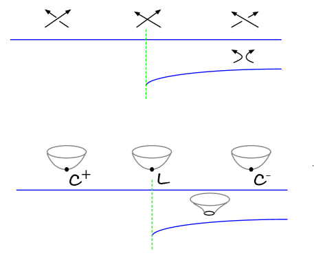
Figure 2. Moduli spaces near nodal curves, top hyperbolic and bottom elliptic. Solid blue lines indicates parameterized moduli spaces of curves, with the interesting parts of the curves depicted above them. The green dashed line indicates the association of points in distinct moduli spaces that leads to the skein relation.

Lemma 4.17.

   

• For generic $J\in\mathcal{J}$ the moduli space ${\mathcal{M}}(J)$ is a transversely cut out compact oriented 0-manifold. For a generic path $\lambda\colon[0,1]\to\mathcal{J}$ the solution space ${\mathcal{M}}(0,1)$ is a compact oriented $1$-manifold with boundary. The boundary consists of ${\mathcal{M}}(0)\cup{\mathcal{M}}(1)$ and a finite number of nodal curves ${\mathcal{M}}(t_{j})$ for $0<t_{1}<\dots<t_{k}<1$. The projection $\pi\colon{\mathcal{M}}(0,1)\to[0,1]$ is a Morse function with interior critical point at non-transverse solutions in ${\mathcal{M}}(t_{s}^{\prime})$ where the dimension of the kernel of the linearized Cauchy-Riemann operator has dimension 1.

• The nodal boundary curves are either hyperbolic or elliptic and the 1-parameter family is locally as in Lemma 4.16. The tangent vector to ${\mathcal{M}}(0,1)$ at a nodal curve on the boundary lies in the kernel of the projection $\pi$, but the second derivative of the projection is non-zero.

Proof.

The first two statements in (a) are direct consequences of (4.5). Consider the boundary of the 1-manifold ${\mathcal{M}}(0,1)$. The boundary of the moduli space corresponds to either going to the boundary in the parameter space or going to the boundary in the space of domains. At the boundary in the space of domains, we find at hyperbolic nodes a curve with non-embedded boundary and at elliptic nodes a curve with an interior point mapping to $L$. The fact that there are isolated points where the kernel of the linearized operator equals 1 and that the 1-parameter family meets the locus of such curves transversely follows again from (4.5). This establishes (a).

We next prove (b): Lemma 4.16 gives the desired normal form of the moduli spaces, the quadratic behavior of the projection map follows from the gluing argument where we invert the differential uniformly on the complement of the gluing parameter and where the constant in the total elliptic estimate blows up at a linear rate in the gluing parameter. This means that the projection map from the moduli space has a quadratic degeneration at its endpoint, see Figure 2. ∎

4.5. Somewhere injectivity and perturbations

We now show that if there is a space of almost complex structures $\mathcal{J}$ such that any $J$-holomorphic curve under consideration is somewhere injective then we can take ${\mathcal{P}}=\mathcal{J}$ to construct a system of perturbations satisfying Definition 4.2. The proof is just to combine our new result on compactness of bare curves with the above-reviewed standard facts on transversality for somewhere injective curves.

Proposition 4.18.

Let $(X,L)$ be as above and let $A\in H_{2}(X,L)$ be a homology class. If $\mathcal{J}$ has the property that every bare $J$-holomorphic curve in homology class $A$ is somewhere injective then we get an integral adequate perturbation scheme by taking ${\mathcal{P}}=\mathcal{J}$ and defining ${\mathcal{M}}(J)$ for $J\in\mathcal{J}$ to be the moduli space of bare $J$-holomorphic curves.

Proof.

We take $\mathcal{P}=\mathcal{J}$, and for $J\in\mathcal{J}$, we take ${\mathcal{M}}(J)$ to be the moduli of $J$-holomorphic bare curves. We must verify that the properties in Definition 4.2 are satisfied for generic points and paths.

1. Holds trivially at all $J\in\mathcal{J}$ since we do not perturb the right hand side of the Cauchy-Riemann equation.

2. Define $\mathcal{P}^{\circ}=\mathcal{J}^{\circ}$ as the subset of generic $J\in\mathcal{J}$ where every solution is transversely cut out, is embedded and in particular has boundary an embedded link, is transverse to the 4-chain $C$, and has interior disjoint from $L$. Then $\mathcal{J}^{\circ}$ is open and dense by Lemmas 4.13, 4.14, and 4.15. By transversality our solution space is an oriented 0-manifold. We define the weights to be given by the orientation, so $w=\pm 1$. Evidently Properties (2b) is satisfied. Property (2c) holds by request, and Property (2d) by transversality.

   We turn to property (2a). It is not simply a consequence of Gromov compactness, since we have taken ${\mathcal{M}}(J)$ the moduli space of bare curves, and not all curves. That is, by Gromov we know that a sequence of bare curves must converge to some stable map; it remains to exclude the possibility that this limit is a non-bare curve. But by Lemma 4.9, such a limit would have underlying bare curve a singular $J$-holomorphic curve, which contradicts property (2c).

3. Lemma 4.17 classifies the degenerations possible in a generic one parameter family. Properties (3b) - (3e) follow immediately.

   We turn to Property (3a). It is not simply a consequence of Gromov compactness, since we have taken ${\mathcal{M}}(J)$ the moduli space of bare curves, and not all curves. By Gromov, a 1-parameter family will have a limit, which may however be a non-bare curve. However, from Lemma 4.9, a limiting non-bare curve will either have a non-immersed point or a triple point in the image of its bare component. By coherence (property (1)), this means that at this $J$, we have a map from a smooth domain with either a triple point or a non-immersed point. This contradicts property (3e).

4. This follows from Lemma 4.16, Lemma 4.14, and coherence.

∎

4.6. Somewhere injectivity for curves in basic homology classes

In this section we construct a class of almost complex structures on $T^{\ast}S^{3}$ for which all bare curves in basic homology classes are somewhere injective. We first consider the cotangent bundle $T^{\ast}S^{3}$ and then the resolved conifold.

Pick a real analytic representative of $K$. Then there are holomorphic coordinates $S^{1}\times(-\eta_{1},\eta_{1})\times B(\eta_{2})$, where $B(\eta_{2})\subset{\mathbb{C}}^{2}$ is an $\eta_{2}$-ball around the origin, on a neighborhood $V_{K}$ of $K$ in $T^{\ast}S^{3}$. Here $S^{3}$ corresponds to $S^{1}\times\{0\}\times(B(\eta_{2})\cap{\mathbb{R}}^{2})$ and $L_{K}$ to $S^{1}\times\{0\}\times(B(\eta_{2})\cap i{\mathbb{R}}^{2})$. Also, the $\epsilon$-shifted $L_{K}$ corresponds to $S^{1}\times\{\epsilon\}\times(B(\eta_{2})\cap i{\mathbb{R}}^{2})$, if $\epsilon<\eta_{1}$.

Consider almost complex structures which agrees with the complex structure in $S^{1}\times(\frac{1}{2}\epsilon,\frac{1}{2}\eta_{1})\times B(\frac{1}{2}\eta_{2})$ inherited from the standard complex structure on $S^{1}\times{\mathbb{R}}\times{\mathbb{C}}^{2}$. We call such almost complex structures $(\eta_{1},\eta_{2})$-normalized.

If $u\colon(\Sigma,\partial\Sigma)\to(T^{\ast}S^{3},L_{K})$ is a bare holomorphic curve then recall we call its homology class basic if its boundary represents the generator $H_{1}(L_{K})$.

Lemma 4.19.

Let $J$ be any $(\eta_{1},\eta_{2})$-normalized almost complex structure. For all sufficiently small shifts $\epsilon>0$, any $J$-holomorphic curve in a basic homology class is somewhere injective.

Proof.

The area of a curve in a basic homology class is $C\epsilon$ for some constant $C>0$. Monotonicity shows that any curve with boundary in $L_{K}$ either outside an $\frac{1}{4}\eta_{1}$-neighborhood of $K$ or with boundary points both outside an $\frac{1}{2}\eta_{2}$-neighborhood and inside an $\frac{1}{4}\eta_{2}$-neighborhood has area $>K\eta_{2}^{2}$ for some $K>0$. It follows that the boundary must lie inside an $\frac{1}{2}\eta_{2}$ neighborhood, if $\epsilon>0$ is sufficiently small.

Consider a boundary component of the curve mapping to $L_{K}$. If we compose the curve near the boundary with the projection to the first coordinate we get a holomorphic map into $(\frac{1}{2}\epsilon,\eta_{1})\times S^{1}$. Since the local degree of this map is non-negative it follows that if the projection is not contained in $(\frac{1}{2}\epsilon,\epsilon]\times S^{1}$ (i.e., if the curve does not lie on one side of the projection of the shifted $L_{K}$) then it must contain points $\{\frac{1}{2}\eta_{1}\}\times S^{1}$. This however contradicts the area bound as above. It follows by Taylor expansion at boundary points that the projection of any boundary component must map to $\{\epsilon\}\times S^{1}$ as a degree one immersion. Then, since the total homology class is one we find that the curve is injective near the boundary. Finally, points not in a neighborhood of the boundary cannot map to points on the boundary again by monotonicity. The lemma follows. ∎

The split complex structure of Lemma 4.19 allows us to control the boundary behavior of any basic curve in any $(\eta_{1},\eta_{2})$-normalized almost complex structure. In order to use the Fredholm theory of Section 4.5 and get the desired transversality of the $\bar{\partial}_{J}$-equation needed for an adequate perturbation scheme we must find a suitable functional analytic neighborhood of the solutions. For bare curves with stable domains this is immediate, we take the Sobolev space of maps into $(X,L)$ with 3 derivatives in $L^{2}$. For stable maps with unstable domains (disks and cylinders) we first stabilize the domains to fix gauge and then proceed in the same way. Given the strong control near the boundary this is straightforward. We use Lemma 4.19 to stablize domains of disks and annuli as follows:

Fix distinct points $p_{j}$, $j=1,2,3$ on the the central circle $S^{1}\times\{\epsilon\}\times 0\subset L_{K}$ and consider the disk fibers $\{p_{j}\}\times i{\mathbb{R}}^{2}\cap B(\eta)$ through these points. Add boundary marked points at the intersections of the curve and these hypersurfaces. This gives stable domains for all curves and we use Sobolev spaces of maps with two derivatives in $L^{2}$ on these domains to give a functional analytic neighborhood of our holomorphic curves. It is straightforward to check, compare [12], that changing the location of the points give smooth coordinate changes on resulting spaces of solutions.

We next consider the case when the target space is the resolved conifold $X$ instead of $T^{\ast}S^{3}$. Fixing a neighborhood of the conormal $L_{K}$ we have exactly the same notion of $(\eta_{1},\eta_{2})$-normalized almost complex structure. We will alter the neighborhood slightly to $S^{1}\times(\eta_{1}^{\prime},\eta_{1})\times B(\eta_{2})$ allowing for a smaller half interval in the direction of the shift. The injectivity result we get requires us to fix the homology class of the map. Fix a splitting $H_{2}(X,L_{K})\to H_{2}(X)$, e.g. by picking capping disks for generators of $H_{1}(L_{K})$. Then any holomorphic curve $u$ in the basic homology class determines a closed 2-cycle $k(u)\cdot[{\mathbb{C}}P^{1}]\in H_{2}(X)$. Let $t$ denote the symplectic area of ${\mathbb{C}}P^{1}$.

Lemma 4.20.

Let $J$ be any $(\eta_{1},\eta_{2})$-normalized almost complex structure and assume that $L_{K}$ is shifted a small distance so that Lemma 4.19 holds. For any $k_{0}$ there exists $t(k_{0})>0$ such that any basic $J$-holomorphic curve $u$ with $k(u)<k_{0}$ is somewhere injective.

Proof.

The proof of Lemma 4.19 with $\frac{1}{2}\epsilon$ applies provided we take $t(k_{0})$ such that $t(k_{0})\cdot k_{0}<\frac{1}{2}\epsilon$. ∎

Remark 4.21.

For our curve counts using only perturbation of $\mathcal{J}$ we must shrink the Kähler parameter as the homology class increases. For homology classes below a fixed bound we can argue exactly as in $T^{\ast}S^{3}$ to stabilize the domains of stable maps near solutions.

4.7. Adequate perturbations for basic curves

We now collect the transversality results above. Let $\mathcal{J}$ denote the space of $(\eta_{1},\eta_{2})$-normalized almost complex structures and let $\epsilon>0$ be sufficiently small for Lemma 4.19 to hold.

Proposition 4.22.

   

• In $T^{\ast}S^{3}$, $\mathcal{P}=\mathcal{J}$ gives an adequate perturbation scheme for basic curves in $T^{\ast}S^{3}$.

• In $X$, for any $k_{0}>0$ there is $t_{0}>0$ such that taking $\mathcal{P}=\mathcal{J}$ gives an adequate perturbation scheme for basic curves $u$ in $X$ with $k(u)<k_{0}$.

Proof.

Follows from Lemmas 4.19 and 4.20 together with Proposition 4.18. ∎

5. Skein valued curve counts

In this section we show that an adequate perturbation scheme leads to invariant skein valued curve counts.

5.1. Definition

Let $X$ be a 3-dimensional Calabi-Yau manifold and let $L=\bigsqcup_{j=1}^{k}L_{j}$ be a Maslov zero Lagrangian, with a brane structure in the sense of Definition 3.3. Fix $d\in H_{2}(X,L)$ and assume given an adequate perturbation setup for $X,L,d$ in the sense of Definition 4.2. Let $\operatorname{Sk}(L)$ be the skein of $L$, in variables $(a,z)$, $a=(a_{1},\dots,a_{k})$.

Definition 5.1.

For $\lambda\in{\mathcal{P}}^{\circ}(X,L)$, we define

$$\langle\!\langle L\rangle\!\rangle_{X,d,\lambda}=\!\!\!\sum_{u\in{\mathcal{M}}(X,L,d,\lambda)}\!\!w(u)\cdot z^{-\chi(u)}\cdot a^{u\OpenHopf L}\cdot\partial u\ \in\ \operatorname{Sk}(L)$$

The sum is over a finite set of points for each coefficient of $z$ by Properties (2a), (2b), with the second of these providing the function $w$. By Property (2c), $\partial u$ is a framed link in $L$, so we may regard it as an element of the skein. Note that in any given homology class, the Euler characteristic of (even a disconnected) representative is bounded above, so the invariant is a Laurent series in $z$.

We emphasize that we count only bare maps from possibly disconnected curves. That is, the image of each irreducible component has nonzero symplectic area.

5.2. Invariance

Theorem 5.2.

For an adequate perturbation scheme $\mathcal{P}$, $\langle\!\langle L\rangle\!\rangle_{X,d,\lambda}$ is independent of $\lambda\in{\mathcal{P}}^{\circ}(X,L)$.

Proof.

It follows from Properties (2d) and (3b) that $\langle\!\langle L\rangle\!\rangle_{X,d,\lambda}$ is locally constant in ${\mathcal{P}}^{\circ}(X,L)$. Consider now any two points $\lambda_{0},\lambda_{1}\in{\mathcal{P}}^{\circ}$, and a path $\lambda_{t}$ connecting them satisfying Property (3). We want to study the $t$ with $\lambda_{t}\notin{\mathcal{P}}^{\circ}$, in order to show that also the count $\langle\!\langle L\rangle\!\rangle_{X,d,\lambda}$ does not change when passing these.

Note that to prove the desired constancy of $\langle\!\langle L\rangle\!\rangle_{X,d,\lambda}$, it is enough to work order by order in $z$. Bounding the order $z$ bounds the genus and holes, thus the set of walls $t_{0}$ we must consider is finite by Property (3d). Fix one such $t_{0}$.

As $t\to t_{0}$, by (2d), the curve counts are locally constant, and the moduli space is just a disjoint union of intervals. By compactness (3a), each such interval has a limit at $t_{0}$. Consider all components for which the limiting curve remains smooth, embedded, transverse to $L$; i.e., (2c) remains true at the limit. Then, even if (2d) fails, nevertheless (3b) suffices to ensure that these components of moduli have the same contribution on both sides of $t_{0}$.

Let us consider the remaining components, i.e., those for which the limiting curve fails (2c). Taking the normalization gives a map from a smooth domain, which is strictly greater Euler characteristic, so among those we are considering at the current order in $z$. Recall there is a unique such map, as per (3c), and that it must take one of the forms classified by Property (3e). Note that since (2c) fails, we have demanded that (2d) does not; i.e. the component of moduli containing this map from a smooth domain locally projects to $[0,1]$ by an isomorphism.

For crossings of ‘framing change’ type, by applying Lemmas 3.8 and 3.9, and comparing to the framing change skein relation, we see that the term $a^{u\OpenHopf L}\cdot\langle\partial u\rangle$ is itself invariant.

We now turn to hyperbolic and elliptic crossings. First, the hyperbolic case. Let $u$ be the map with smooth domain and nodal image, and $u_{\times}$ the corresponding embedding of a nodal curve. We will write $u_{\pm\epsilon}$ for the curves immediately before and after $u$ in its family, and $u$ for the deformation of $u_{\times}$ which appears on one side (either before or after). We write $w(u_{\bullet})$ for the degree of the 0-chain on the corresponding moduli space.

According to Property 3c, curves unrelated to $u$ undergo no critical moments. The 4-chain intersection and $H_{2}(X,L)$ of all the $u_{\bullet}$ are the same. Thus the total change in $\langle\!\langle L\rangle\!\rangle_{X,L,\lambda}$ is a multiple of

$$w(u_{\epsilon})z^{-\chi(u_{\epsilon})}\langle\partial u_{\epsilon}\rangle\ -\ w(u_{-\epsilon})z^{-\chi(u_{-\epsilon})}\langle\partial u_{-\epsilon}\rangle\pm\ w(u)z^{-\chi(u)}\langle\partial u\rangle.$$

By Properties 3b and 2d, $w(u_{\epsilon})=w(u_{-\epsilon})$. By Property 4 this quantity is also equal to $w(u)$. In addition, note that $\chi(u_{\epsilon})=\chi(u_{-\epsilon})=\chi(u)+1$. Thus the above discrepancy is a multiple of

(5.1) $$\langle\partial u_{\epsilon}\rangle\ -\ \langle\partial u_{-\epsilon}\rangle\ \pm\ z\langle\partial u\rangle,$$

Recall that Property (4) asks that the crossing moment is locally given by the model in Section 4.1, in the sense of Definition 4.1. Inspection of the hyperbolic model shows that the images of the boundary under $u_{\pm\epsilon}$ differ precisely by a crossing change $\overcrossing\leftrightarrow\undercrossing$, whereas the boundary of $u$ is correspondingly the .

Now let us consider the elliptic crossing. We use similar notations as above, save writing $u_{\bigcirc}$ instead of $u$. The same considerations apply, with one exception: $u_{\pm\epsilon}$ have one more or one less intersection with the 4-chain than $u_{\circ}$ does. Thus now the relation is

$$a^{\pm 1}\langle\partial u_{\epsilon}\rangle\ -\ a^{\mp 1}\langle\partial u_{-\epsilon}\rangle\ \pm\ z\langle\partial u_{\bigcirc}\rangle.$$

Again inspecting the model in Section 4.1, the difference between the boundaries is that $\partial u_{\bigcirc}$ has an extra unknot as compared to $\partial u_{\pm\epsilon}$, the latter two being isotopic to each other. Thus, the above expression is a multiple of

(5.2) $$a\ -\ a^{-1}\ \pm\ z\langle\bigcirc\rangle.$$

It remains to fix the signs on $z$ in the formulas (5.1) and (5.2).

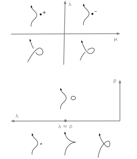
Figure 3. Relation between hyperbolic and elliptic nodes near a cusp.

Consider the 2-parameter family of holomorphic maps defined for $\zeta$ in a neighborhood of the origin in the upper half plane $\{z=s+it\in{\mathbb{C}}\colon y\geq 0\}$, see Figure 3, upper part:

$$z\mapsto\left(\zeta^{2},\zeta(\zeta^{2}+\lambda),\mu\zeta\right),$$

where $(\lambda,\mu)$ lies in a neighborhood of the origin in ${\mathbb{R}}^{2}$. For $\mu=0$, $\lambda<0$ the holomorphic map has a hyperbolic boundary crossing and for $\mu=0$, $\lambda>0$ the curve has an elliptic boundary crossing. Consider the 1-parameter family of curves with $\mu\neq 0$ fixed and $\lambda$ changing sign. Such a family corresponds to a framing change and we know that the curve count in the framed skein module does not change.

Consider next the lower part of Figure 3. Here we depict the $\lambda$-axis as the boundary of another family of holomorphic curves of Euler characterstic one smaller. For generic $\lambda$ and $\rho$ the boundary is as depicted. For $\lambda<0$ the distance between the components shrinks faster than the radius of the circle, for $\lambda>0$ the circle shrinks faster, and at $\lambda=0$ they shrink at the same rate and we limit to a cuspidal curve.

We conclude from these pictures that $\pm z$ times the curve at $(\lambda,\rho)$, $\rho>0$ equals both the elliptic and the hyperbolic crossing differences. Thus, changing $z$ to $-z$ in our original conventions if necessary, we may ensure that the sign in formula (5.1) is $+$ and in formula (5.2) is $-$. With this choice, formulas (5.1) and (5.2) are simply the skein relations, hence zero in the skein. ∎

It follows immediately from Theorem 5.2 that if we have an adequate perturbation setup for all $d$ then we have invariance of

(5.3) $$Z_{X,L,\lambda}:=1+\sum_{d>0}\langle\!\langle L\rangle\!\rangle_{X,d,\lambda}\cdot Q^{d}\in Sk(L)\otimes{\mathbb{Q}}[[H_{2}(X,L)]]$$

Remark 5.3.

Rather than simply discard holomorphic curves with collapsed components, a more typical approach is to perturb the Cauchy-Riemann equation to $\partial u=\epsilon$ even on curves with zero symplectic area, thus ensuring that no curve will literally map to a point. Let us explain why this sort of approach is not compatible with the ideas above. The first difficulty is for the framing change. We used the standard behavior near the boundary to identify with the standard tangency family, where we calculated that framing changes and 4-chain intersections cancel as they should. However, for a perturbed solution of zero symplectic area there is no natural way to ensure this standard holomorphic behavior near the boundary without making the perturbation ‘large’. This means that one cannot guarantee the right framing behavior. Thinking of the family around the cusped curve (Figure 3), it is clear that these problems will propagate through the perturbation scheme. Thus, even when we turn to more general perturbation methods in [11], we will not perturb the Cauchy-Riemann equation on components with zero symplectic area, and instead again discard curves with such components as we have done here.

5.3. Closed and open invariants

Let us consider the empty Lagrangian. Now $Z_{X}$ is just the usual closed Gromov-Witten count of disconnected curves (which is the exponential of the series most commonly considered in the mathematics literature), re-expressed as count of bare curves. We can define a reduced invariant $Z_{X,L}/Z_{X}$; it is independent of choices because both numerator and denominator are. However, it does not generally have a direct and invariant enumerative intepretation: it may happen that closed curves have nonvanishing intersection number with the 4-chain for $L$, hence contribute differently to the numerator and denominator. However:

Lemma 5.4.

Assume $\lambda\in{\mathcal{P}}^{\circ}(X,L)$ is such that every closed $\lambda$-holomorphic curve has zero intersection number zero with the 4-chain for $L$. Then

$$Z_{X,L,\lambda}/Z_{X,\lambda}=1+\sum w(u)\cdot z^{-\chi(u)}\cdot Q^{u_{*}[\Sigma]}\cdot a^{u\OpenHopf L}\cdot\langle\partial u\rangle\ \in\ \operatorname{Sk}(L)[[Q]],$$

where the sum is taken only over bare curves $u\in{\mathcal{M}}(X,L)$ such that every component of the domain is a curve with boundary.

Proof.

Immediate from the definitions. ∎

Remark 5.5.

We consider an example to illustrate consequences of counting in the skein module. When we take into account the 4-chain, the contributions of closed curves which intersect the 4-chain cannot be invariantly separated from those of open curves with contractible boundary. For example, suppose that we have found generic perturbation data such that there are no curves with boundary on $L$ and that no closed curve intersects the 4-chain. Then $Z_{X,L}/Z_{X}$ counts only actual curves with boundary. There are no such, so $Z_{X,L}/Z_{X}=1$. Now deform the data, e.g. the 4-chain, in such a way that there is an instance when the 4-chain becomes tangent to one of the closed curves. After this instance that closed curve intersects the 4-chain in two points with opposite intersection signs. After further deformation one of these intersection points moves to the boundary $L$ of the 4-chain and at an elliptic crossing a new holomorphic curve with boundary on $L$ is born. After this moment there is a unique nondegenerate curve with boundary on $L$. Nevertheless its contribution is cancelled by that of closed curves, and it remains the case that $Z_{X,L}/Z_{X}=1$.

6. SFT and the conifold transition

In this section we compare curve counts in $T^{*}S^{3}$, in $T^{*}S^{3}\setminus S^{3}$, and in the resolved conifold $X$. The key ingredient is SFT compactness and the stretching arguments it makes possible.

6.1. The conifold transition

Let us review the conifold transition. Consider the locus $X_{0}=\{w^{2}+x^{2}+y^{2}+z^{2}=0\}$ in ${\mathbb{C}}^{4}$. On the one hard, this locus is the image of the total space of the bundle $X={\mathcal{O}}(-1)\oplus{\mathcal{O}}(-1)$ over ${\mathbb{C}}P^{1}$, under a map which collapses the ${\mathbb{C}}P^{1}$ and is elsewhere an embedding. On the other hand, there is the deformation $X_{\epsilon}=\{w^{2}+x^{2}+y^{2}+z^{2}=\epsilon\}$, which is symplectomorphic to $T^{*}S^{3}$. The conifold transition means we replace one with the other.

From a symplectic point of view, $X_{\epsilon}$ provides an exact symplectic filling of the contact cosphere bundle $S^{*}S^{3}$. This means that outside of a compact $X_{\epsilon}$ agrees with the the positive symplectization $[0,\infty)\times S^{\ast}S^{3}$ with its standard symplectic form $d(e^{t}\,pdq)$, where $pdq$ is the action form restricted to $S^{\ast}S^{3}$ and $t$ a coordinate on $[0,\infty)$. The resolved conifold is not quite a symplectic filling of $S^{\ast}S^{3}$. However, far from the central ${\mathbb{C}}P^{1}$, also $\tilde{X}$ looks topologically like $[0,\infty)\times ST^{\ast}S^{3}$ and the symplectic form is deformation equivalent to $d(e^{t}\,pdq)+\omega$, where $\omega$ is independent of $t$. For large $t$ this can be viewed as a small perturbation that vanishes in the limit $t\to\infty$. We say that $X$ is an asymptotic symplectic filling of $S^{\ast}S^{3}$. We also use the notion asymptotically convex at infinity for symplectic manifolds with positive ends that are asymptotic to symplectizations of contact manifolds in the above sense. Similarly, we say that a Lagrangian $L\subset X$ is asymptotically Legendrian at infinity if it is asymptotically close in the same sense to the symplectization ${\mathbb{R}}\times\Lambda$ of a Legendrian $\Lambda\subset S^{\ast}S^{3}$. See [29] for basic results about holomorphic curves in this setting.

From topological string theory [56, 18, 19, 38] comes the prediction that the Chern-Simons theory on $S^{3}$ should be equivalent to topological string theory on $X_{\epsilon}=T^{*}S^{3}$ with $N$ branes along the zero section, which in turn should be equivalent to topological string theory in $X$. Here the number $N$ of branes in $X_{\epsilon}$ is supposed to be related by a change of variables to a parameter measuring the area of the ${\mathbb{C}}P^{1}$.

In our setup, we do not explicitly have a ‘number of branes’. Instead we have the 4-chain, and the resulting Lagrangian linking number it determines. Indeed, if one were to imagine taking $N$ branes, it would mean in our context having $N$ times the 4-chain, hence multiplying the linking number by $N$. Thus we expect a change of variables replacing our $a$ variable counting linking with the $S^{3}$ with a $Q$ variable counting $H_{2}$ class along the ${\mathbb{C}}P^{1}$. Indeed consider a conical-at-infinity 4-chain $C\subset T^{*}S^{3}$, with as usual $\partial C=2S^{3}$. At infinity, such a class is Poincaré dual to twice the generator of $H_{2}(S^{\ast}S^{3})$.

6.2. SFT stretching near Lagrangian submanifolds

In this section we review SFT-stretching in the context we will require it. Let $L\subset X$ be a Lagrangian. We consider a family of almost complex structures $J_{s}$, $s\in[0,\infty)$ on $X$ as follows. Recall that a neighborhood $N$ of $L$ can be symplectically identified with a neighborhood of the 0-section $L$ inside $T^{\ast}L$. We think of this neighborhood $N$ as the unit disk cotangent bundle $D_{1}T^{\ast}L$. For $s\in[0,\infty)$, we consider the following three symplectic manifolds:

$$X^{+}_{s} =(X-N)\cup_{\partial N}((-s,0]\times ST^{\ast}L_{K}),$$

$$X^{0}_{s} =[-s,s]\times ST^{\ast}L,$$

$$X^{-}_{s} =N\cup\partial N([0,s)\times ST^{\ast}L),$$

where we equip the symplectization pieces with the same ${\mathbb{R}}$-invariant almost complex structure and denote it $J_{s}^{\prime}$. Define

$$X_{s}=X^{+}_{s}\cup_{\tau_{2s}}X^{-}_{s},$$

where $\tau_{2s}(\sigma,y)=(\sigma+2s,y)$ is the conformally symplectic map that intertwines the symplectic structure $d(e^{\sigma}\alpha)$ with $d(e^{\sigma+2s}\alpha)$. Shrinking the neighborhood $N$ slightly we can identify $X$ with $X_{\epsilon}$ for small $\epsilon>0$ and define diffeomorphisms $\phi_{s}\colon X_{s}\to X$ by shrinking $X^{0}_{s}$ to $X^{0}_{\epsilon}$. Via these diffeomorphisms we can transport $J_{s}^{\prime}$ to a family $J_{s}$ of almost complex structures on $X$, all compatible with the symplectic structure $\omega$: $J_{s}=d\phi_{s}\circ J^{\prime}_{s}\circ d\phi_{s}^{-1}$.

We next state the SFT-compactness theorem adapted to our situation. Consider a Lagrangian $L^{\prime}\subset X$ disjoint from a small neighborhood of $L$. Let $u_{s}$, $s\to\infty$ be a sequence of $J_{s}$-holomorphic curves with boundary on $L^{\prime}$ and of uniformly bounded area.

Proposition 6.1.

[5] There exists a subsequence $u_{s^{\prime}}$ that converges to a holomorphic building in $X^{-}_{\infty}$, $X^{0}_{\infty}$, and $X^{+}_{\infty}$, where the levels are joined at Reeb orbits in $S^{\ast}L$. Furthermore, the total action of the Reeb orbits at the negative ends of the curves in $X_{\infty}^{+}$ is bounded in terms of the symplectic area of the curves. If the action of Reeb orbits in $ST^{\ast}L$ is uniformly bounded from below it follows in particular that the holomorphic building is finite.∎

Consider SFT stretching around $L$. Consider a Riemannian metric $g$ on $L$ and the induced contact 1-form $\alpha_{g}$ on the unit cotangent bundle $ST^{\ast}L$. The Reeb flow of $\alpha_{g}$ is the lift of the geodesic flow of $g$ and the Conley-Zehnder index of a Reeb orbit equals the Morse index of the corresponding geodesic. The most important cases to us are the following.

Example 6.2.

If $L\approx S^{3}$ and we equip $S^{3}$ with the standard round metric then the closed geodesics come in Bott families, of which the minimal index is $2$. It follows that after a small perturbation, still the minimal index of a geodesic is $2$.

Example 6.3.

If $L\approx S^{1}\times{\mathbb{R}}^{2}$ then there is a metric with a unique geodesic loop that goes once around the generator of $\pi_{1}(S^{1}\times{\mathbb{R}}^{2})$. All other geodesic loops are multiples of this basic loop, and all closed Reeb orbits have Conley-Zehnder index $0$.

We next consider consequences of SFT stretching for general adequate perturbation schemes. More precisely, we consider such schemes for the ambient space $X^{+}_{\infty}$. We assume further that the negative end of $X_{\infty}^{+}$ is modeled on $S^{\ast}S^{3}$ with contact form corresponding to the round metric. We require in addition to the properties in Definition 4.2 that the curves are unperturbed holomorphic in some neighborhood of the negative end.

Lemma 6.4.

Let $L\subset X^{+}_{\infty}$ be a Lagrangian and let $\gamma$ be a collection of Reeb orbits in $S^{\ast}S^{3}$. Then in generic 1-parameter families there is no holomorphic curve in $X^{+}_{\infty}$ with negative asymptotics at $\gamma$. It follows in particular that skein valued curve counts for $(X_{\infty}^{+},L)$ can de defined exactly as in Definition 5.1 and Theorem 5.2 holds.

Proof.

The dimension of such a curve would be the negative of the index of $\gamma$. By transversality the corresponding moduli space is then empty over generic 1-parameter families. It then follows that the degeneracies in 1-parameter families are exactly as in the case without negative end. ∎

Remark 6.5.

Note that in the above argument, transversality for curves in an SFT setup was used to argue that moduli spaces which should have negative codimension are in fact empty. For the curves in the lemma, this is nothing fancy; as noted our choices force somewhere-injectivity. However, to make the analogous argument in the context of curves in more general homology classes (or if one does not want to impose our requirements on the complex structure near $L$), one needs a perturbation setup which ensures the relevant SFT transversality.

With Lemma 6.4 established we first relate curve counts in $(T^{\ast}S^{3},S^{3})$ and $T^{\ast}S^{3}\setminus S^{3}$ and then compare curve counts in $T^{\ast}S^{3}\setminus S^{3}$ and the resolved conifold $X$. We have the following results.

We say that $L$ is a Lagrangian brane in $T^{*}S^{3}\setminus S^{3}$ to mean that the 4-chain can be chosen to lie entirely in $T^{*}S^{3}\setminus S^{3}$. Recall from Remark 2.9 our conventions for coefficients in $T^{*}S^{3}$ and $T^{*}S^{3}\setminus S^{3}$.

Theorem 6.6.

Let $L$ be a Lagrangian brane in $T^{*}S^{3}\setminus S^{3}$. Then:

(6.1) $$Z_{T^{*}S^{3},S^{3}\cup L}(a,a_{L},z)=Z_{T^{*}S^{3}\setminus S^{3},L}(Q,a_{L},z)\big{|}_{Q=a^{2}}\otimes[\varnothing_{S^{3}}]\in\operatorname{Sk}(S^{3})$$

Proof.

It suffices to establish this equality order by order in $z$ and thus we may fix area and Euler characteristic bounds. Write $N(r)$ for an radius $r$-neighborhood of $S^{3}\subset T^{\ast}S^{3}$.

Consider the curves contributing to $Z_{T^{*}S^{3},S^{3}\cup L}$. Let $\epsilon>0$ be sufficiently small so that $L$ lies outside $N(10\epsilon)$. We apply SFT-stretching near $\partial N(5\epsilon)$. By Lemma 6.4 for sufficiently large stretching parameter $\rho$ we find an almost complex structure $J_{\rho}$ such that all curves with boundary on $L$ lies outside $N(5\epsilon)$. Furthermore, all closed $J_{\rho}$-holomorphic curves have zero symplectic area and are therefore constant.

That is, we may deform the complex structure for $T^{*}S^{3}$ so that all curves leave a neighborhood of the $S^{3}$. Now the curves contributing to the invariant are literally the same for $(T^{*}S^{3},S^{3}\cup L)$ and $(T^{*}S^{3}\setminus S^{3},L)$ (see Lemma 6.4 for the latter count); it remains only to examine how we count them. In the former case we must account for the intersection with the 4-chain; in the latter case, for the class in $H_{2}(T^{*}S^{3}\setminus S^{3})$. These match under the substitution $Q=a^{2}$, since generating homology class in $H_{2}(T^{*}S^{3}\setminus S^{3})$ is dual to half of the 4-chain, viewed as an element of $H_{4}^{BM}(T^{*}S^{3}\setminus S^{3})$. ∎

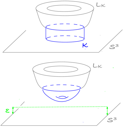
Figure 4. Top picture shows the unique annulus with boundary on $L_{K}$ and along $K\subset S^{3}$, before SFT-stretching. As we SFT-stretch, the boundary on $S^{3}$ undergoes skein moves until, as illustrated in the bottom picture, all curves left an $\epsilon$-neighborhood of $S^{3}$.

Theorem 6.7.

Let $L$ be a Lagrangian brane in $T^{*}S^{3}\setminus S^{3}$. Then we consider $L$ as a brane also in $X$ and

(6.2) $$Z_{T^{*}S^{3}\setminus S^{3},L}(Q,a_{L},z)=\frac{Z_{X,L}(Q,a_{L},z)}{Z_{X}(Q,z)}$$

Proof.

Again it suffices to establish this equality order by order in $z$ and thus we may fix area and Euler characteristic bounds. Basically the point will be to apply Lemma 5.4 on the RHS, which we may do once we can ensure the closed curves avoid the 4-chain. We will also need to relate the complex structure appropriate to the non-exact symplectic form on $\widetilde{X}$ to one appropriate to the exact symplectic form on $T^{*}S^{3}\setminus S^{3}$.

We next construct an almost complex structures on $\widetilde{X}$ which give arbitrarily small perturbations of $J_{\rho}$ on $T^{\ast}S^{3}\setminus N(5\epsilon)$ as follows. Write $\tilde{X}_{\delta}$ for $\tilde{X}$ with central ${\mathbb{C}}P^{1}$ or area $\delta>0$. Note that for the standard almost complex structure all holomorphic curves in $\widetilde{X}$ maps to the central sphere. Therefore, all perturbed holomorphic curves maps to an arbitrarily small neighborhood of it.

Let $B$ be a radius $1$ neighborhood of ${\mathbb{C}}P^{1}$ in $\widetilde{X}_{\delta}$. For $\delta=0$, $\widetilde{X}_{\delta}$ is a cone and its symplectic structure near $\partial B$ can after scaling be identified with that in $T^{\ast}S^{3}$ near $\partial N(\epsilon)$. For small $\delta$ we can use the same identification, however, to make the symplectic forms match we must add a $\delta$-multiple of the closed 2-form dual to the fiber.

Note next that the almost complex structure $J_{\rho}$ is not compatible with this new symplectic form. We change it to a compatible almost complex structure $J_{\rho,\delta}$ by adding a linear operator of size $\delta$. By transversality all (perturbed, bare) $J_{\rho}$-holomorphic curves in $T^{\ast}S^{3}$ with boundary on $L$ are transversely cut out. Hence for $\delta>0$ sufficiently small all $J_{\rho,\delta}$-holomorphic curves are transversely cut out as well and moreover canonically identified with the $J_{\rho}$-holomorphic curves.

Consider small $\delta>0$ so that this identification of curves applies. Note that both the standard almost complex structure on $B$ and $J_{\rho,\delta}$ give almost complex structures on $N(5\epsilon)\setminus N(4\epsilon)$ that are compatible with the symplectic form on $\widetilde{X}$. Interpolating between the two gives a compatible almost complex structure $J_{\delta}$ on $\widetilde{X}$.

We claim that for all sufficiently small $\delta>0$ all (perturbed) $J_{\delta}$-holomorphic curves that contributes to the numerator in the right hand side of (6.2) are either $J_{\delta}$-holomorphic curves in $T^{\ast}S^{3}\setminus N(5\epsilon)$ with boundary on $L$, or holomorphic curves contained in a small neighborhood of the central ${\mathbb{C}}P^{1}$, or constant. To see this, consider first a closed curve. Since the minimal area of a cycle in the homology class $[{\mathbb{C}}P^{1}]$ outside a suitable small neighborhood of ${\mathbb{C}}P^{1}$ is $>2\delta$ and the area of any holomorphic curve equals its symplectic area there can be no non-constant holomorphic curves outside a small neighborhood of ${\mathbb{C}}P^{1}$. Assume next that there exist a $J_{\delta}$-holomorphic curve with boundary on $L$ that intersects $N(5\epsilon)$-neighborhood. Consider a sequence of such curves as $\delta\to 0$ and $\rho\to\infty$. By SFT-compactness the level of the limiting curve with boundary on $L$ would be a holomorphic curve in ${\mathbb{R}}\times ST^{\ast}S^{3}$ with negative punctures at a Reeb orbit. As in Lemma 6.4 such a curve would have negative dimension and therefore does not exist by transversality.

We have thus shown that for $\rho>0$ and $\delta>0$ all closed (perturbed) $J_{\delta}$-holomorphic curves in $\widetilde{X}$ have image in a small neighborhood of the middle ${\mathbb{C}}P^{1}$, and in particular avoid the 4-chain associated to $L$. ∎

Remark 6.8.

We have written Theorems 6.6 and 6.7 collecting together all homology classes, but really they are making independent statements for the coefficient of each monomial in $a_{L}$. To fully justify the statement for a particular monomial, it suffices to construct an adequate perturbation scheme for that particular homology class. Thus, for the coefficient corresponding to curves in the basic homology class, these theorems are established unconditionally, using Proposition 4.22.

7. Enumerative meaning of the HOMFLYPT polynomial

Let $K=K_{1}\cup\dots\cup K_{k}\subset S^{3}$ be a link, and let $L_{K}$ its conormal Lagrangian, shifted off the $0$-section. We first note the following.

Lemma 7.1.

The conormal to a link defines a Lagrangian brane in $T^{*}S^{3}\setminus S^{3}$.

Proof.

Such a conormal is disjoint from a cotangent fiber, hence null-homologous in $T^{\ast}S^{3}\setminus S^{3}$, hence bounds a 4-chain there. ∎

Thus we may apply Theorems 6.6 or 6.7 to relate the curve counts on $L_{K}\cup S^{3}\subset T^{*}S^{3}$ with those of $L_{K}\subset T^{*}S^{3}$ or $L_{K}\subset\widetilde{X}$, respectively. It remains to actually compute $Z_{T^{*}S^{3},L_{K}\cup S^{3}}$. This invariant takes values in a tensor product of skein modules of $S^{3}$ and solid tori $S^{1}\times{\mathbb{R}}^{2}$. Recall the skein of $S^{3}$ is just the free rank one module over the coefficient ring, generated by the class of the empty knot $\varnothing$. This assertion is essentially equivalent to the existence of the HOMFLYPT polynomial $\langle K\rangle_{S^{3}}\in{\mathbb{Z}}[a^{\pm},z^{\pm}]$ of links $K$:

$$K=\langle K\rangle_{S^{3}}\,\cdot\,\varnothing\in\operatorname{Sk}(S^{3}).$$

For the solid torus $S^{1}\times{\mathbb{R}}^{2}$, we recall from [49] that $\operatorname{Sk}(S^{1}\times{\mathbb{R}}^{2})$ is a free polynomial algebra over ${\mathbb{Z}}[a^{\pm},z^{\pm}]$ with generators indexed by the integers.

$$\operatorname{Sk}(S^{1}\times{\mathbb{R}}^{2})\cong{\mathbb{Z}}[a^{\pm},z^{\pm}][\ldots,\ell_{-2},\ell_{-1},\ell_{0},\ell_{1},\ell_{2},\ldots].$$

The algebra can be viewed as a ${\mathbb{Z}}$-graded, with $\deg(\ell_{i})=i$; the grading records the class in $H_{1}(S^{1}\times{\mathbb{R}}^{2})$ determined by the skein representative. We write $\operatorname{Sk}^{+}(S^{1}\times{\mathbb{R}}^{2})$ and $\operatorname{Sk}^{-}(S^{1}\times{\mathbb{R}}^{2})$ for the subalgebras on the positive and negative generators; $\operatorname{Sk}(S^{1}\times{\mathbb{R}}^{2})=\operatorname{Sk}^{+}(S^{1}\times{\mathbb{R}}^{2})\otimes\operatorname{Sk}^{-}(S^{1}\times{\mathbb{R}}^{2})$. Then $\operatorname{Sk}^{+}(S^{1}\times{\mathbb{R}}^{2})$ is a free ${\mathbb{Z}}[a^{\pm},z^{\pm}]$ module on a basis naturally indexed by partitions. In fact there is a natural identification of $\operatorname{Sk}^{+}(S^{1}\times{\mathbb{R}}^{2})$ with the ring of symmetric functions, but we will not need it here.

In particular, if we fix a basis for the skein of the solid torus, e.g. monomials in the $\ell_{i}$, then we may extract the corresponding coefficients of $Z_{T^{*}S^{3},S^{3}\cup L_{K}}$; said coefficient will take values in $\operatorname{Sk}(S^{3})$. Here we will focus just on the simplest term. We fix the generator $\ell=\ell_{1}$ represented by $S^{1}\times\{0\}$ and write $1^{k}\in{\mathbb{Z}}^{k}=H_{1}(L_{K})=H_{2}(T^{*}S^{3},S^{3}\cup L_{K})$ for the homology class which is the sum of these generators for all components.

We will now make a particular choice of 4-chain in order to avoid framing ambiguities in the statements of theorems. Changing the 4-chain affects the invariants by monomial factors and monomial changes of variable. We will also construct explicit capping chains that gives the correct normalization for connecting our curve count to the framed HOMFLYPT in Theorem 1.1. The capping chains will also allow us also to define the linking number $u\OpenHopf L$ in this setting without reference to the intersection $\gamma=L_{K}\cap C$.

Fix $\xi$ a non-zero vector field on $S^{3}$ which is nowhere tangent to the link $K$. Consider the $4$-chain $C_{\xi}$ which is the union of the positive and negative half rays determined by $\xi$ and oriented in such a way that $\partial C_{\xi}=2[S^{3}]$. Consider the conormal $L_{K}$ shifted along a closed 1-form dual to the tangent vector of the knot. Then the central curve $\beta_{j}=S^{1}\times 0\subset L_{K}$ is disjoint from $C$. Recall that $\beta=\sum_{j}\beta_{j}$ and pick a chain $\sigma^{\prime}\subset T^{\ast}S^{3}\setminus S^{3}$ with $\partial\Sigma^{\prime}=\beta$ which is transverse to $C$. Define

$$\sigma_{\xi}^{\prime}=\sigma^{\prime}-\tfrac{1}{2}(\sigma^{\prime}\cdot C)F,$$

where $\sigma^{\prime}\cdot C$ denotes the algebraic intersection number of $\sigma^{\prime}$ and $C$ and where $F$ denotes a fiber 2-sphere in $T^{\ast}S^{3}\setminus S^{3}$. Then

$$\sigma_{\xi}^{\prime}\cdot C=0.$$

Remark 7.2.

We point out that $\sigma_{\xi}$ depends on $\xi$: if we deform $\xi$ in a 1-parameter family with a standard transverse tangency to $K$ at some point then the intersection number $\sigma^{\prime}\cdot C$ changes by $\pm 1$ and $\sigma_{\xi}$ changes accordingly by $\mp F$.

For later convenience we will further specify the local behavior of $\sigma_{\xi}$ near $K\subset L_{K}$. We will show in Lemma 4.19 that for almost complex structures standard near $L_{K}$ there are coordinates $S^{1}\times(-\epsilon,\epsilon)\times B(\epsilon)$, where $B(\epsilon)$ is a ball in ${\mathbb{C}}^{2}$, where $L_{K}$ corresponds to $S^{1}\times{\mathbb{R}}^{2}\cap B(\epsilon)$, and where every holomorphic curve we consider agrees with the standard cylinder $S^{1}\times(-\epsilon,0]\times\{p\}$, where $p\in{\mathbb{R}}^{2}$. We will take our capping chain $\sigma_{\xi}$ that caps such a holomorphic curve to agree with $S^{1}\times[0,\epsilon)\times\{p\}$. It is clear that one can construct a smoothly varying family of such capping chains (varying only near the boundary) parameterized by $p\in B(\epsilon)$. Our capping chains $\sigma_{\xi}$ will have this property.

The restricted boundary behavior of the holomorphic curves we count in the setting of Theorem 1.1 allows us to simplify the definition of linking. Consider the original definition (3.1):

$$u\OpenHopf L:=u_{J\nu}\cdot C+\partial u\OpenHopf\gamma.$$

For $C=C_{\xi}$, $\gamma\cap S^{3}=\varnothing$. Using capping chains $\sigma_{\xi}$ as above we will write $\overline{u}_{J\nu}=u_{J\nu}\cup\sigma_{\xi}$ and replace the above definition by

(7.1) $$u\OpenHopf S^{3}:=\overline{u}_{J\nu}\cdot C.$$

Since $\overline{u}_{J\nu}$ is a 2-chain with boundary disjoint from $\partial C$ this is well defined. Invariance under deformations follows as before except that the analogue of Lemma 3.8 is simpler. In the present case an intersection point moves from $u$ to $\sigma_{\xi}$ and the intersection number is clearly preserved.

In order to relate (7.1) to (3.1) we need first to understand the intersection $\gamma=L_{K}\cap C$. To this end we first look at the intersection $\gamma^{\prime}=L_{K}^{\prime}\cap C\subset T^{\ast}S^{3}$ where $L_{K}^{\prime}$ denotes the unshifted conormal. It is easy to see that $\gamma^{\prime}=K\cup_{p}\xi(p)^{\ast}_{\pm}$, where $p$ denotes the points where the tangent to $K$ is perpendicular to $\xi$ and $\xi^{\ast}_{\pm}$ denotes the positive and negative half-lines in the fiber of the conormal of $K$ at the point $p$ in direction of the co-vector dual to $\xi$. For the shifted conormal the intersection $\gamma$ is a smoothing of the curve $\gamma^{\prime}$ that is disjoint from the central copy of $K$. We see in particular that $\gamma$ has (ideal) boundary and in order to use (3.1) we pick paths at infinity closing $\gamma$ up. To define linking with $\gamma$ we then fix bounding chains as described in [9]. For a suitable choice of bounding chains (3.1) and (7.1) give the same result. In fact, one such choice is obtained by using as bounding chains of $\gamma$ the flow lines starting on $\gamma$ of a Bott-function with a minimum along the central circle $K\subset L_{K}$: since the boundary of all holomorphic curves in the basic class lie close to the central circle there are no contributions form linking with $\gamma$ which corresponds to no intersections between the 4-chain and the capping disk.

Fix the capping chain $\sigma_{\xi}$ and use (7.1) as the definition of linking number with $S^{3}$.

Let $J$ be an $(\eta_{1},\eta_{2})$-normalized almost complex structure on $T^{\ast}S^{3}\setminus S^{3}$.

Theorem 7.3.

We have the following equality in $\operatorname{Sk}(S^{3}\cup L_{K})$:

$$\langle\!\langle S^{3}\cup L_{K}\rangle\!\rangle_{T^{*}S^{3},1^{n}}=K\otimes\ell^{\otimes n}$$

Proof.

Recall from the definition of $(\eta_{1},\eta_{2})$-normalized complex structures, see Section 4.6 that there is an obvious holomorphic cylinder given in local coordinates by $S^{1}\times[-\epsilon,0]\times\{0\}$. We claim that it is unique in the basic homotopy class.

Assume that there is a boundary point of the curve passing through a point $p\in S^{3}\cup L_{K}$ outside $N(\frac{1}{2}r)$, then, provided $r$ is sufficiently small, there is ball of radius $\frac{1}{4}r$ around $p$ that intersects $L$ in a disk. By monotonicity, it then follows that the area of the curve is larger than $Cr^{2}$ for some constant $C$, but the area of the curve is bounded by $C^{\prime}\delta$ so for sufficiently small $\delta>0$ the boundary of the curve lies inside $N(\frac{1}{2}r)$. Assume now that there is an interior point that maps to a point $q$ outside $N(\frac{1}{2}r)$. Then we find a ball of radius $\frac{1}{4}r$ around $q$ that contains no boundary point of the curve. Montonicity then implies that the area of the curve is $>Cr^{2}$ which again gives a contradiction for small enough $\delta$. We conclude that any curve lies inside $N(r)$. Let $u$ be such a curve then we compose $u$ with the local coordinate projection to the $(z_{1},z_{2})$-plane. The boundary of the projection then maps to ${\mathbb{R}}\times{\mathbb{R}}$ and we find that the area of the projection is either constant or at least $\frac{1}{4}\pi\rho^{2}$, where $\rho$ is the radius of coordinate disk contained in our neighborhood. It follows that the projection of the curve to the $(z_{1},z_{2})$-plane is constant. It is easy to see that the curve must then be the standard annulus $A$ in the first coordinate.

It remains to check that $A$ is transversely cut out. The linearization of the $\bar{\partial}$-operator at $A$ is simply the standard $\bar{\partial}$-operator with boundary condition in ${\mathbb{R}}\times{\mathbb{R}}^{2}$ along on boundary component and ${\mathbb{R}}\times i{\mathbb{R}}^{2}$ along the other, there is a constant solution in the ${\mathbb{R}}$-direction (the linearization of rotations along $A$) and no solutions in the other directions. It follows that the curve is transversely cut out.

It follows that the cylinders $A$ for each knot component of $K$ are the only curves in the class of the generator. Thus the coefficient of $\ell\otimes\ell\otimes\cdots\otimes\ell$ is just the count of the union of these singly covered cylinders. A cylinder has Euler characteristic zero, so there are no constant curve contributions. Furthermore, by definition of $\sigma_{\xi}$ the linking number of the cylinder and $S^{3}$ equals zero and hence the count is just 1 times the boundary in $S^{3}$, which is the original link $K$ itself, $\langle K\rangle\in\operatorname{Sk}(S^{3})$. ∎

Corollary 7.4.

Using the bounding chain $\sigma_{\xi}$ to define linking, we have the following equality in $\operatorname{Sk}(L_{K})$.

$$\sum_{d}\langle\!\langle L_{K}\rangle\!\rangle_{T^{*}S^{3}\setminus S^{3},1^{n}\oplus d}=\langle K\rangle_{S^{3}}\cdot\ell^{\otimes n}.$$

Proof.

Follows from Theorem 7.3 and Theorem 6.6. ∎

Remark 7.5.

The curve counts in Theorem 7.3 and Corollary 7.4 can be reinterpreted as counts of curves without boundaries as follows. Consider a Riemannian metric on the $S^{1}\times{\mathbb{R}}^{2}$-components of $L_{K}$ with a single minimizing geodesic at $S^{1}\times\{0\}$ and SFT-stretch around $L_{K}$ equipped with this metric. It is straightforward to check that the only curves in connected components of $T^{\ast}L_{K}$ which have boundary on the zero section and which are asymptotic to the Reeb orbit $\gamma$ that corresponds to the geodesic which is a positive homology generator are the cylinders over this geodesic. Since this SFT-stretching is a modification of the almost complex structure near $L_{K}$ it follows that the counts in Theorem 7.3 and Corollary 7.4 can be identified with the count of punctured curves in $T^{\ast}S^{3}\setminus(S^{3}\cup L_{K})$. Here $\ell^{\otimes n}$ should be substituted by $\gamma^{\otimes n}$, i.e., the curves counted have negative punctures where it is asymptotic to the simple positive Reeb orbits in the components of $L_{K}$.

Proof of Theorem 1.1.

We may now deduce Theorem 1.1 from Corollary 7.4 and Theorem 6.7 together with Lemma 4.19 that shows that the boundary of any holomorphic curve in a basic homology class is a longitude and Lemma 4.20 that gives somewhere injectivity for sufficiently small Kähler parameters. ∎

Appendix A Physical origin of the 4-chain

In this section we give a brief motivation from M-theory of the 4-chain used to define the linking number with $L$. Recall that Chern-Simons theory on the 3-manifold $L$ is concerned with the path integral

$$\int\mathcal{D}A\,e^{\frac{ki}{4\pi}\operatorname{CS}(A)},$$

where the functional integral is over gauge equivalence classes of $U(N)$-connections $A$, and

$$\operatorname{CS}(A)=\int_{M}\operatorname{tr}\left(A\wedge dA+\tfrac{2}{3}A\wedge A\wedge A\right).$$

If $X$ is a Calabi-Yau 3-fold and $L\subset X$ is a Lagrangian then in topological string theory one considers $L$ as a boundary condition for open strings. Here there are gauge fields in the form of $U(1)$ connections living on $L$, and $L$ with such a connection is called a brane. More generally one considers $N$ coincident branes along $L$. Then the dynamics of short strings stretching between the branes is goverened by $U(N)$ gauge theory along $L$ and the end points of strings couple ’electrically’ to these gauge fields.

As explained in [56], in $T^{\ast}L$ where there are no non-constant instantons the string field theory reduces to a theory on the space of the low energy super symmetric states which in this case is simply the space of constant maps or $L$ itself, and the string field theory action becomes the Chern-Simons action. Considering next $L\subset X$, where $X$ contains non-constant holomorphic curve $u$ with boundary $\partial u$, [56] integrates out the contribution form the non-constant curve and arrives at a theory on $L$ with effective action.

$$\operatorname{CS}(A)\ +\ e^{\operatorname{area}(u)}g_{s}^{\chi(u)}\operatorname{tr}(\mathrm{Hol}_{\partial u}(A)),$$

where $\operatorname{area}(u)$ is the symplectic area of $u$ and $\mathrm{Hol}_{\partial u}$ is the holonomy along the boundary. Expanding the exponential in the path integral this means that the partition function is multiplied by the insertion of the Wilson loop of all disjoint curves corresponding to $u$.

This is what we have tried to capture with the skein valued Gromov-Witten invariants. However, there is a disparity: the above-described quantity seems not to be invariant under deformations. Specifically, consider stretching as in Theorem 6.6 so that boundaries of the curves are forced to disappear. In that case the partition function clearly changes by the HOMFLYPT polynomial of the disappearing link.

Our skein invariants remain invariant and what is missing is the contributions from the 4-chain intersections. To see where these originate from physically, we turn to M-theory. In this set up M-theory lives in the 11-dimensional space $X\times S^{1}\times{\mathbb{R}}^{4}$, and our theory is a reduction of this theory to $X$. In M-theory there are M2 branes with 3-dimensional world sheets and M5 branes with 6-dimensional world sheets. The Lagrangian $L\subset X$ originates from an M5 brane on $L\times S^{1}\times{\mathbb{R}}^{2}$ and the holomorphic curves $u$ originates from M2 branes on $u\times S^{1}$. The M5 brane is the source of a 3-form that couples electrically to M2 branes. More precisely, there is a 4-form field strength $G_{4}$ that is a solution to the equation

$$dG_{4}=j_{M5},$$

where $j_{M5}$ is a Dirac 5-form in the directions normal to the $M5$-brane, and the 3-form $A_{3}$ satisfies

$$dA_{3}=G_{4}.$$

The electric coupling is then simply $\int_{M2}A_{3}$.

From a topological view point we can represent the field strength $G_{4}$ by a $7$-chain with boundary $M5$ thought of as a family of Dirac strings emanating from M5. The 3-form $A_{3}$ then measures linking with this 7-chain and thus corresponds to intersections with another family of Dirac strings emanating from the 7-chain, compare e.g. [30].

After reduction this leaves a magnetic (linking) coupling between $L$ and holomorphic curves roughly corresponding to the second family of Dirac strings. We denote the corresponding field strength $G_{2}$. This gives another term in the deformation of Chern-Simons theory which then looks like:

$$CS(A)+e^{\operatorname{area}(u)}g_{s}^{\chi(u)}\mathrm{tr}(\mathrm{Hol}_{\partial u}(A))+\int_{u}G_{2}.$$

It is not immediate to make sense out of this formula since the boundary of the holmorphic curve goes right through the source of $G_{2}$ which is the reduction of $A_{3}$.

Similarly, in the case that the $4$-chain $C$ intersects $L$ there is a similar extra term in the path integral that corresponds to defects of the connections along the curve $\gamma$ of intersection. The correction originates from the term $A_{3}\wedge G_{4}\wedge G_{4}$ in the M-theory action, or in other words the dual of $G_{4}\wedge G_{4}$ that interacts electrically with M2 branes, or more geometrically the self-intersections of the 7-chain of Dirac strings is a 3-dimensional object that affects M2 branes like other M2 branes.

References

- [1] Mina Aganagic, Tobias Ekholm, Lenhard Ng, Cumrun Vafa, et al. Topological strings, d-model, and knot contact homology. Advances in Theoretical and Mathematical Physics, 18(4):827–956, 2014.
- [2] Mina Aganagic, Albrecht Klemm, Marcos Marino, and Cumrun Vafa. The topological vertex. Communications in mathematical physics, 254(2):425–478, 2005.
- [3] Anna Aiston and Hugh Morton. Idempotents of Hecke algebras of type . J. Knot Theory Ramifications, 7(4):463–487, 1998.
- [4] Johan Björklund. Flexible isotopy classification of flexible links. J. Knot Theory Ramifications, 25(8):1650049, 9, 2016.
- [5] Frederic Bourgeois, Yakov Eliashberg, Helmut Hofer, Kris Wysocki, and Eduard Zehnder. Compactness results in symplectic field theory. Geom. Topol., 7:799–888, 2003.
- [6] Kai Cieliebak, Kenji Fukaya, and Janko Latschev. Homological algebra related to surfaces with boundary. arXiv preprint arXiv:1508.02741, 2015.
- [7] Duiliu-Emanuel Diaconescu, Vivek Shende, and Cumrun Vafa. Large N duality, Lagrangian cycles, and algebraic knots. Communications in Mathematical Physics, 319(3):813–863, 2013.
- [8] Tobias Ekholm. The complex shade of a real space, and its applications. Algebra i Analiz, 14(2):56–91, 2002.
- [9] Tobias Ekholm and Lenhard Ng. Higher genus knot contact homology and recursion for colored HOMFLY-PT polynomials. arXiv preprint arXiv:1803.04011, 2018.
- [10] Tobias Ekholm, Lenhard Ng, and Vivek Shende. A complete knot invariant from contact homology. Inventiones mathematicae, pages 1–52, 2018.
- [11] Tobias Ekholm and Vivek Shende. Counting bare curves. in preparation.
- [12] Tobias Ekholm and Ivan Smith. Exact Lagrangian immersions with a single double point. J. Amer. Math. Soc., 29(1):1–59, 2016.
- [13] Bohan Fang and Zhengyu Zong. Topological recursion for the conifold transition of a torus knot. arXiv preprint arXiv:1607.01208, 2016.
- [14] Peter Freyd, David Yetter, Jim Hoste, WB Raymond Lickorish, Kenneth Millett, and Adrian Ocneanu. A new polynomial invariant of knots and links. Bulletin of the American Mathematical Society, 12(2):239–246, 1985.
- [15] Kenji Fukaya. Counting pseudo-holomorphic discs in Calabi-Yau 3-folds. Tohoku Math. J. (2), 63(4):697–727, 2011.
- [16] Kenji Fukaya, Yong-Geun Oh, Hiroshi Ohta, and Kaoru Ono. Lagrangian intersection Floer theory: anomaly and obstruction. American Mathematical Soc., 2010.
- [17] Penka Georgieva. Open Gromov-Witten disk invariants in the presence of an anti-symplectic involution. Adv. Math., 301:116–160, 2016.
- [18] Rajesh Gopakumar and Cumrun Vafa. On the gauge theory/geometry correspondence. arXiv preprint hep-th/9811131, 1998.
- [19] Rajesh Gopakumar and Cumrun Vafa. Topological gravity as large N topological gauge theory. arXiv preprint hep-th/9802016, 1998.
- [20] Tom Graber and Eric Zaslow. Open-string Gromov-Witten invariants: Calculations and a mirror theorem. arXiv preprint hep-th/0109075.
- [21] Richard Hadji and Hugh Morton. A basis for the full Homfly skein of the annulus. Math. Proc. Cambridge Philos. Soc., 141(1):81–100, 2006.
- [22] Helmut Hofer, Kris Wysocki, and Eduard Zehnder. Properties of pseudoholomorphic curves in symplectisations. I. Asymptotics. Ann. Inst. H. Poincaré Anal. Non Linéaire, 13(3):337–379, 1996.
- [23] Vito Iacovino. Open Gromov-Witten theory on Calabi-Yau three-folds I. arXiv:0907.5225, 2009.
- [24] Vito Iacovino. Open Gromov-Witten theory on Calabi-Yau three-folds II. arXiv:0908.0393, 2009.
- [25] Vito Iacovino. Open Gromov-Witten theory without obstruction. arXiv:1711.05302, 2017.
- [26] Vaughan Jones. A polynomial invariant for knots via von Neumann algebras. Bull. Am. Math. Soc., 12:103–111, 1985.
- [27] Sheldon Katz and Chiu-Chu Melissa Liu. Enumerative geometry of stable maps with lagrangian boundary conditions and multiple covers of the disc. Geometry & Topology Monographs, 8:1–47, 2006.
- [28] Kenichi Kawagoe. On the skeins in the annulus and applications to invariants of -manifolds. J. Knot Theory Ramifications, 7(2):187–203, 1998.
- [29] Sergiy Koshkin. Conormal bundles to knots and the Gopakumar-Vafa conjecture. Adv. Theor. Math. Phys., 11(4):591–634, 2007.
- [30] Kurt Lechner, Pieralberto Marchetti, and Mario Tonin. Anomaly free effective action for the elementary M5-brane. Physics Letters B, 524(1-2):199–207, 2002.
- [31] Jun Li, Chiu-Chu Melissa Liu, Kefeng Liu, and Jian Zhou. A mathematical theory of the topological vertex. Geom. Topol., 13(1):527–621, 2009.
- [32] Chiu-Chu Melissa Liu. Moduli of J-holomorphic curves with Lagrangian boundary condition and open Gromov-Witten invariants for an -pair. arXiv preprint math/0210257.
- [33] Sascha Lukac and Hugh Morton. The HOMFLY polynomial of the decorated Hopf link. Journal of Knot Theory and Its Ramifications, 12(03):395–416, 2003.
- [34] Marcos Mariño. Chern-Simons theory and topological strings. Rev. Modern Phys., 77(2):675–720, 2005.
- [35] Hugh Morton and Peter Samuelson. The HOMFLYPT skein algebra of the torus and the elliptic Hall algebra. Duke Math. J., 166(5):801–854, 2017.
- [36] Jun Murakami. The parallel version of polynomial invariants of links. Osaka J. Math., 26(1):1–55, 1989.
- [37] Andrei Okounkov and Rahul Pandharipande. Hodge integrals and invariants of the unknot. Geom. Topol., 8:675–699, 2004.
- [38] Hirosi Ooguri and Cumrun Vafa. Knot invariants and topological strings. Nucl.Phys., B577:419–438, 2000, hep-th/9912123.
- [39] Rahul Pandharipande. Hodge integrals and degenerate contributions. Communications in Mathematical Physics, 208(2):489–506, 1999.
- [40] Rahul Pandharipande, Jake Solomon, and Johannes Walcher. Disk enumeration on the quintic 3-fold. J. Amer. Math. Soc., 21(4):1169–1209, 2008.
- [41] Grisha Perelman. Ricci flow with surgery on three-manifolds. arXiv preprint math/0303109, 2003.
- [42] Józef Przytycki. Skein modules of -manifolds. Bull. Polish Acad. Sci. Math., 39(1-2):91–100, 1991.
- [43] Józef Przytycki and Pawel Traczyk. Invariants of links of conway type. Kobe journal of mathematics, 4:115–139, 1988.
- [44] Nicolai Reshetikhin. Quantized universal enveloping algebras, the Yang-Baxter equation and invariants of links. LOMI-preprint E-4-87 and E-17-87, 1988.
- [45] Vivek Shende. The conormal torus is a complete knot invariant. Forum of Mathematics, Pi, 7, 2019.
- [46] Jean-Claude Sikorav. Some properties of holomorphic curves in almost complex manifolds. In Holomorphic curves in symplectic geometry, volume 117 of Progr. Math., pages 165–189. Birkhäuser, Basel, 1994.
- [47] Jake Solomon. Intersection theory on the moduli space of holomorphic curves with lagrangian boundary conditions. arXiv preprint math/0606429.
- [48] Jake Solomon and Sara Tukachinsky. Differential forms, Fukaya algebras, and Gromov-Witten axioms. arXiv preprint arXiv:1608.01304.
- [49] Vladimir Turaev. The Conway and Kauffman modules of a solid torus. Zap. Nauchn. Sem. Leningrad. Otdel. Mat. Inst. Steklov. (LOMI), 167(Issled. Topol. 6):79–89, 190, 1988.
- [50] Vladimir Turaev. The Yang-Baxter equation and invariants of links. Inventiones mathematicae, 92(3):527–553, 1988.
- [51] Vladimir Turaev. Skein quantization of Poisson algebras of loops on surfaces. Ann. Sci. École Norm. Sup. (4), 24(6):635–704, 1991.
- [52] Oleg Viro. Encomplexing the writhe. In Topology, ergodic theory, real algebraic geometry, volume 202 of Amer. Math. Soc. Transl. Ser. 2, pages 241–256. Amer. Math. Soc., Providence, RI, 2001.
- [53] Jean-Yves Welschinger. Open Gromov-Witten invariants in dimension six. Math. Ann., 356(3):1163–1182, 2013.
- [54] Hans Wenzl. Representations of braid groups and the quantum Yang-Baxter equation. Pacific J. Math., 145(1):153–180, 1990.
- [55] Edward Witten. Quantum field theory and the Jones polynomial. Communications in Mathematical Physics, 121(3):351–399, 1989.
- [56] Edward Witten. Chern-Simons gauge theory as a string theory. Prog.Math., 133:637–678, 1995, hep-th/9207094.