Robust Temporal Difference Learning for Critical Domains

Abstract.

We present a new Q-function operator for temporal difference (TD) learning methods that explicitly encodes robustness against significant rare events (SRE) in critical domains. The operator, which we call the $\kappa$-operator, allows to learn a robust policy in a model-based fashion without actually observing the SRE. We introduce single- and multi-agent robust TD methods using the operator $\kappa$. We prove convergence of the operator to the optimal robust Q-function with respect to the model using the theory of Generalized Markov Decision Processes. In addition we prove convergence to the optimal Q-function of the original MDP given that the probability of SREs vanishes. Empirical evaluations demonstrate the superior performance of $\kappa$-based TD methods both in the early learning phase as well as in the final converged stage. In addition we show robustness of the proposed method to small model errors, as well as its applicability in a multi-agent context.

1. Introduction

Many critical systems exhibit global system dynamics that are highly sensitive to the local performance of individual components. This holds for example for (air) traffic and transport networks, communication networks, security systems, and (smart) power grids (Cristian et al., 1996; Shooman, 2003; Knight, 2002; Liu et al., 2012). In each case, the failure of or malicious attack on a small set of nodes may lead to knock-on effects that can potentially destabilise the whole system. Innovations in critical systems may introduce additional vulnerabilities to such attacks: e.g., in smart grids communication channels are needed for distributed intelligent energy management strategies, while simultaneously forming a potential target that could compromise safety (Yan et al., 2013). Our research is motivated precisely by the need for safety in these critical systems, which can be achieved by building in robustness against rare but significant deviations caused by one or more system components failing or being compromised in an attack.

In this article we present a new approach for learning policies in such systems that are robust against a chosen scenario of potential attacks or failures. We accomplish this by introducing a new Q-function operator, which we call the $\kappa$-operator, that encodes robustness into the bootstrapping update of traditional temporal difference (TD) learning methods. In particular, we design the operator to encode the possibility of significant rare events (SREs) without requiring the learning agent to observe such events in training. Although the $\kappa$-operator is model-based with respect to these SREs, it can be combined with any TD method and can thus still be model-free with respect to the environment dynamics.

We prove convergence of our methods to the optimal robust Q-function with respect to the model using the theory of Generalized Markov Decision Processes. In addition we prove convergence to the optimal Q-function of the original MDP given that the probability of SREs vanishes. Empirical evaluations demonstrate the superior performance of $\kappa$-based TD methods both in the early learning phase as well as in the final converged stage. In addition we show robustness of the proposed method to small model errors, as well as its applicability to multi-agent joint-action learning.

This articles proceeds with related work in Section 2 and background concepts in Section 3. We formally introduce the new TD operator $\kappa$ in Section 4 and subsequently prove convergence. Section 6 provides empirical results, and Section 7 concludes.

2. Related Work

The aim to find robust policies is relevant to multiple research areas, including security games, robust control/learning, safe reinforcement learning and multi-agent reinforcement learning.

The domain of security games has expanded in recent years with many real-world applications in critical domains (Pita et al., 2008; Shieh et al., 2012), where the main approach has been computing exact solutions and deriving strong theoretical guarantees, mostly using equilibria concepts such as Nash and Stackelberg equilibria (Korzhyk et al., 2011; Lou et al., 2017). In contrast, we base our approach on reinforcement learning from interactions with the environment, thus we do not need to know the system model; such an approach to security games has been studied less, exceptions being for example Ruan et al. (2005) and Klima et al. (2016) who use reinforcement learning in the context of patrolling and illegal rhino poaching problems, respectively. Security games often assume frequent adversarial attack, whereas our work focuses on occasional loss of control over the system, which can represent e.g. failures or adversarial attack. Moreover, our work adopts the information asymmetry assumption often used in Stackelberg Security games (Korzhyk et al., 2011), providing the model of attack types for the leader, and allowing leader-strategy-informed best response strategies by attackers. Similar to security games, control theory starts with a model of the system to be controlled (the plant), and for the purpose of robust control assumes a set of possible plants as an explicit model of uncertainty, seeking to design a policy that stabilises all these plants (Zhou and Doyle, 1998). A slightly weaker assumption is made in related work that assumes control over the number of observations for significant rare events (SREs), performing updates by sampling from the model (Ciosek and Whiteson, 2017). In contrast, our work assumes that the model of this system is not known a priori, and a policy needs to be learned by interacting with it. While early work on robust reinforcement learning focused on learning within parameterised acceptable policies (Singh et al., 1994), later work transferred the objective of maximising tolerable disturbances from control theory to reinforcement learning (Morimoto and Doya, 2005). Our work is similar to the therein defined Actor-disturber-critic, but we replace its model of minimax simultaneous actions with stochastic transitions between multiple controllers (one being in control at any time) with arbitrary objectives for each controller. In relation to the taxonomy of safe reinforcement learning of Garcıa and Fernández (2015) our method falls in between Worst-Case Criterion under Parameter Uncertainty and Risk-Sensitive Reinforcement Learning Based on the Weighted Sum of Return and Risk, depending on the chosen alternate controller objectives. Our Q($\kappa$) method is comparable to the $\beta$-pessimistic Q-learning method of Gaskett (2003), however, we propose a more general $\kappa$ operator of which Q($\kappa$) is only an example. Finally, our approach has commonalities with the multi-agent reinforcement learning algorithm Minimax-Q (Littman, 1994) for zero-sum games, which assumes minimisation over the opponent action space. However, in contrast, we define an attack to minimise over our own action space, and thus learn (but not enact) simultaneously our optimal policy and the (rare) attacks it is susceptible to. We further cover not only minimising adversaries but also random failures or any other policy encoding other adversaries’ agendas (see Section 4.1).

3. Background

This work belongs to the field of reinforcement learning (RL) Sutton and Barto (2018), and makes use of the core concept of a Markov decision process (MDP). An MDP is formally defined by a tuple $(S,A,R,P)$, where $S$ is a finite set of states, $A$ is a finite set of actions, $R(s,a)\rightarrow r\in\mathbb{R}$ is the reward function for a given state $s\in S$ and an action $a\in A$ and $P(s^{\prime}|s,a)$ is the transition function giving a probability of reaching state $s^{\prime}$ after taking action $a$ in state $s$. In this work we also consider a multi-agent setting, which uses the formalism of the stochastic game, which generalizes the MDP to multiple agents and is defined by a tuple $(n,S,A_{1}\ldots A_{n},R_{1}\ldots R_{n},P)$, where $n$ is the number of agents and $A_{i}$ is the action space of agent $i$. The joint action space is $A=A_{1}\cup\ldots\cup A_{n}$, and a joint action is $\bm{a}=(a_{1},a_{2},\ldots,a_{n})$. $R_{i}(s,a_{i},\bm{a_{-i}})\rightarrow r_{i}$ is the reward function of agent $i$ for given state $s$ and joint action $\bm{a}$, and $P(s^{\prime}|s,\bm{a})$ is the state transition function.

The main goal of RL is finding an optimal policy for given MDP. A common method is temporal difference (TD) learning, which estimates the value of a state by bootstrapping from the value-estimates of successor states using Bellman-style equations. TD methods work by updating their state-value estimates in order to reduce the TD error, which describes the difference between the current estimate of the (state-)value and a new sample obtained from interacting with the environment. In this work we focus on modifying the update target of this TD error, which has the standard form of $r+\gamma V(s^{\prime})$, where $\gamma$ is the discount factor and $V(s^{\prime})$ is the current estimate of the next state’s value. In on-policy methods such as SARSA the target is induced by the actual (behaviour) policy being followed, while off-policy methods use an alternative operator (e.g., greedy maximization as in Q-learning). We refer the reader to Sutton and Barto (2018) for an overview of RL.

4. The Robust TD Operator $\kappa$

Before we formally define our robust TD operator $\kappa$, we give an intuitive example. Suppose a Q-learning agent needs to learn a robust policy against a potential malicious adversary who could, with some probability $\varkappa$, take over control in the next state. The value of the next state $s_{t+1}$ thus depends on who is in control: if the agent is in control, she can choose an optimal action that maximizes expected return; or if the adversary is in control he might, in the worst case, aim to minimize the expected return. This can be captured by the following modified TD error

$$\delta_{t}=r_{t+1}+\gamma\left((1-\varkappa)\max_{a}Q(s_{t+1},a)+\varkappa\min_{a}Q(s_{t+1},a)\right)-Q(s_{t},a_{t}),$$

where we assume that the agent has knowledge of (or can estimate) the probability $\varkappa$.

In the following we first present a formal, general model of the operator $\kappa$, by modifying the target in the standard Bellman style value function. We then present practical implementations of TD($\kappa$) methods that use this operator, for both single- and multi-agent settings, based on the classical on- and off-policy TD learning algorithms (Expected) SARSA and Q-learning.

4.1. Formal Model

We consider a set of $m$ possible control policies $C=\{\sigma_{1},\ldots,\sigma_{m}\}$. At each time step, one of these policies is in control (and thus decides on the next action) with some probability $p(\sigma_{i}|s)$ that may depend on the state $s$. The set $C$ and probability function $p(\cdot)$ are assumed to be (approximately) known by the agent. In our new TD methods, the value of the next state $s^{\prime}$ then becomes a function of both the state and the function $p(\cdot)$, which we capture in our proposed operator $\kappa$ as $V^{\kappa}(s^{\prime})$. Note that the set $C$ includes the focal policy $\pi$ that we seek to optimise in face of (possibly adversarial) alternative controllers. Such external control policies can represent for example a malicious attacker, aiming to minimize the expected return, or any arbitrary dynamics, such as random failures (e.g. represented by a uniformly random policy). Based on a prior assumption about the nature of $\sigma$ we want to optimise the focal policy $\pi$ without necessarily observing actual attacks or failures. This means learning our robust policy $\pi$ right from the start.

We define $\sigma$ in terms of our own Q-value function, for example an attacker that is minimising our expected return. Thus we need to learn only one Q-value function $Q^{\pi}$. This is similar to the standard assumption in Stackelberg games that the attacker is able to fully observe our past actions and thus can enact the informed best response. We define the Q-value function update for our policy $\pi$ based on standard Bellman equation and given the operator $\kappa$ as

$$Q^{\pi}(s,a)\leftarrow Q^{\pi}(s,a)+\alpha\Big{[}\underbrace{r+\gamma V^{\kappa}({s}^{\prime})}_{\textrm{target}}-Q^{\pi}(s,a)\Big{]}.$$ (1)

Note that where in the standard Bellman equation we would have $V^{\pi}(s)=\sum_{a}\pi(s,a)Q^{\pi}(s,a)$, in our case we have

$$V^{\kappa}(s)=\sum_{\sigma\in C}p(\sigma|s)\sum_{a}\sigma(s,a)Q^{\pi}(s,a),$$ (2)

computed as a weighted sum over all possible control policies $\sigma\in C$. Note that we can learn $Q^{\pi}$ without actually experiencing any attack or malfunction, based only on prior assumptions about the possible control policies as captured by the operator $\kappa$. We refer to this target modification as the operator $\kappa$ because it closely resembles the Bellman optimality operator $\mathcal{T}^{\star}$, which is defined as $\mathcal{T}^{\star}V(s)=\max_{a}\big{[}R(s,a)+\sum_{s^{\prime}}P(s^{\prime}|s,a)\gamma V(s^{\prime})\big{]}$. Thus, we can then formally define the $\kappa$ optimality operator $\mathcal{T}^{\star}_{\kappa}$ by substituting the value function $V(\cdot)$ with $V^{\kappa}(\cdot)$.

In the following we present several $\kappa$-versions of classical TD methods. For simplicity we assume a scenario in which we have only a single adversarial external policy $\sigma$ that aims to minimize our value, and thus $C=\{\pi,\sigma\}$. Note however that our model is general, and would work for any $C$ and $p(\cdot)$.

4.2. Examples of TD($\kappa$) Methods

We first present single-agent $\kappa$-based learning methods by building on the standard TD methods Q-learning and Expected SARSA. Then we present two-agent joint-action learning approaches. Although a generalization to $n$ agents is relatively straightforward, we choose to focus solely on the single- and two-agent case in this paper for clarity of exposition. In each case, we consider the setting in which either the focal agent, with policy $\pi$, is in control, or the external adversary with policy $\sigma$ aiming to minimize return. We further simplify the model by making the control policy probability function $p(\cdot)$ state-independent, reducing it to a probability vector.

4.2.1. Single-Agent Methods

Before we present the algorithms, it is important to note that we need to distinguish the target and behaviour policies. The $\kappa$-operator is defined on the target (see Eq. (1)), while the behaviour policy is used only for selecting actions. We assume an $\epsilon$-greedy behaviour policy throughout.

In off-policy Q($\bm{\kappa}$), the target policy is the greedy policy $\pi(s)=\operatorname*{arg\,max}_{a}Q(s,a)$ that maximizes expected return. The adversarial policy on the other hand aims to minimize the return, i.e., $\sigma(s)=\operatorname*{arg\,min}_{a}Q(s,a)$. Assuming a probability of attack of $\varkappa$ as before, we have $p(\pi)=(1-\varkappa)$ and $p(\sigma)=\varkappa$. Thus, Eq. (2) becomes

$$V^{\kappa}(s)=(1-\varkappa)\max_{a}Q(s,a)+\varkappa\min_{a}Q(s,a).$$

For on-policy Expected SARSA($\bm{\kappa}$) the target is the (expectation over the) focal policy $\pi$, while the adversarial policy $\sigma$ remains the same as before. Thus, we have

$$V^{\kappa}(s) =(1-\varkappa)\mathbb{E}_{a\sim\pi}\big{[}Q(s,a)\big{]}+\varkappa\min_{a}Q(s,a)$$

$$=(1-\varkappa)\sum_{a}\pi(a|s)Q(s,a)+\varkappa\min_{a}Q(s,a).$$

4.2.2. Multi-Agent Methods

We move from a single-agent setting to a scenario in which multiple agents interact. For sake of exposition we only present a two-agent case with different action spaces, $A_{1}$ and $A_{2}$, but an identical reward function and thus a shared joint action Q-value function $Q:S\times A_{1}\times A_{2}\rightarrow\mathbb{R}$. Moreover, we assume full communication during the learning phase, allowing the agents to take each other’s policies into account when selecting the next action. Our algorithms are therefore based on the joint-action learning (JAL) paradigm Claus and Boutilier (1998). We further assume that only one agent can be attacked at each time step. For multi-agent Q($\bm{\kappa}$) we can write Eq. (2) for each individual agent as

$$V^{\kappa}(s)=(1-\varkappa)\max_{A_{1}}\max_{A_{2}}Q(s,\langle a_{1},a_{2}\rangle) +\frac{\varkappa}{2}\,\min_{A_{1}}\max_{A_{2}}Q(s,\langle a_{1},a_{2}\rangle)$$

$$+\frac{\varkappa}{2}\,\min_{A_{2}}\max_{A_{1}}Q(s,\langle a_{1},a_{2}\rangle)$$

with $a_{1}\in A_{1}$ and $a_{2}\in A_{2}$, representing the scenario in which no attack happens with probability $(1-\varkappa)$, and each agent is attacked individually with probability $\nicefrac{{\varkappa}}{{2}}$. Analogously, we can define Eq. (2) for multi-agent Expected SARSA($\bm{\kappa}$) as

$$V^{\kappa}(s) =(1-\varkappa)\qquad\mathbb{E}_{a_{1}\sim\pi_{1},a_{2}\sim\pi_{2}}\big{[}Q(s,\langle a_{1},a_{2}\rangle)\big{]}$$

$$+\quad\frac{\varkappa}{2}\quad\,\min_{A_{1}}\mathbb{E}_{a_{2}\sim\pi_{2}}\big{[}Q(s,\langle a_{1},a_{2}\rangle)\big{]}$$

$$+\quad\frac{\varkappa}{2}\quad\,\min_{A_{2}}\mathbb{E}_{a_{1}\sim\pi_{1}}\big{[}Q(s,\langle a_{1},a_{2}\rangle)\big{]}$$

where we now compute an expectation over the actual policy of the agents that are not attacked, while the attacker is still minimizing.

5. Theoretical Analysis

In this section we analyze theoretical properties of the proposed $\kappa$-methods. We start by relating the different algorithms to each other in the limit of their respective parameters. Then we proceed to show convergence of both Q($\kappa$) and Expected SARSA($\kappa$) to two different fixed points: (i) to the optimal value function $Q^{\star}$ of the original MDP in the limit where $\varkappa\rightarrow 0$; and (ii) to the optimal robust value function $Q^{\star}_{\kappa}$ of the MDP that is generalized w.r.t. the operator $\kappa$ for constant parameter $\varkappa$. Note that optimality in this sense is purely induced by the relevant operator. In (i) this is the standard Bellman optimality which maximizes the expected discounted return of the MDP. However, in (ii) we derive optimality in the context of Generalized MDPs Szepesvari and Littman (1997), where optimal simply means the fixed point of a given operator, which can take many forms.

Before proceeding with the convergence proofs, Figure 1 summarizes some relationships between the algorithms in terms of their targets, in the limit of their respective parameters: As is known, Expected SARSA, SARSA, and Q-learning become identical in the limit of a greedy policy (Sutton and Barto, 2018; van Seijen et al., 2009). Furthermore, the update targets of our $\kappa$-methods approach the update targets of the standard TD methods on which they are based as $\varkappa\rightarrow 0$. Finally, Expected SARSA($\kappa$) and Q($\kappa$) share the same relationship as their original versions, and thus Expected SARSA($\kappa$) approaches Q($\kappa$) as $\epsilon\rightarrow 0$. Note that the algorithms’ equivalence in the limit does not hold in the transient phase of the learning process, and hence in practice they may converge on different paths and to different policies that share the same value function. For a comprehensive understanding of the algorithms introduced in Section 4.2, the following sections provide proofs for both convergence of $\kappa$ methods for $\varkappa\rightarrow 0$, as well as their convergence when $\varkappa$ stays constant.

Figure 1. The relationship between the learning targets of different algorithms in the limits of their parameters. On-policy methods are in green, off-policy methods in orange.

5.1. Convergence to the Optimal $Q^{\star}$

There exist several proofs of convergence for the temporal difference algorithms Q-learning Jaakkola et al. (1994); Tsitsiklis (1994), SARSA Singh et al. (2000), and Expected SARSA van Seijen et al. (2009). Each of these proofs hinges on linking the studied algorithm to a stochastic process, and then using convergence results from stochastic approximation theory Dvoretzky (1956); Robbins and Monro (1951). These proofs are based on the following lemma, presented as Theorem 1 in Jaakkola et al. (1994) and as Lemma 1 in Singh et al. (2000). These differ in the third condition, which describes the contraction mapping of the operator. The contraction property used for the Q-learning proof Jaakkola et al. (1994) has the form $||\mathbb{E}\{F_{t}(\cdot)|P_{t}\}||\leq\gamma||\Delta_{t}||$, where $\gamma\in[0,1)$. We show the lemma as it was used for the SARSA proof provided by Singh et al. (2000), who show that the contraction property does not need to be strict; strict contraction is required to hold only asymptotically.

Lemma

Consider a stochastic process $(\alpha_{t},\Delta_{t},F_{t}),t\geq 0$, where $\alpha_{t},\Delta_{t},F_{t}:X\rightarrow\mathbb{R}$ satisfy the equations

$$\Delta_{t+1}(x)=\big{(}1-\alpha_{t}(x)\big{)}\Delta_{t}(x)+\alpha_{t}(x)F_{t}(x),\,x\in X,\,t=0,1,2,\dots$$

Let $P_{t}$ be a sequence of increasing $\sigma$-fields such that $\alpha_{0}$ and $\Delta_{0}$ are $P_{0}$-measurable and $\alpha_{t},\Delta_{t}$ and $F_{t-1}$ are $P_{t}$-measurable, $t=1,2,\dots$. Then, $\Delta_{t}$ converges to zero with probability one (w.p.1) under the following assumptions:

1. the set $X$ is finite,

2. $0\leq\alpha_{t}(x_{t})\leq 1$, $\sum_{t}\alpha_{t}(x_{t})=\infty$, $\sum_{t}\alpha^{2}_{t}(x_{t})<\infty$ w.p.1,

3. $||\mathbb{E}\{F_{t}(\cdot)|P_{t}\}||\leq\gamma||\Delta_{t}||+c_{t}$, where $\gamma\in[0,1)$ and $c_{t}$ converges to zero w.p.1,

4. $Var\{F_{t}(x_{t})|P_{t}\}\leq K(1+||\Delta_{t}||)^{2}$, where $K$ is some constant,

where $||\cdot||$ denotes a maximum norm.

The proof continues by relating Lemma 5.1 to the temporal difference algorithm, following the same reasoning as van Seijen et al. (2009) in their convergence proof for Expected SARSA. We define $X=S\times A$, $P_{t}=\{Q_{0},s_{0},a_{0},r_{0},\alpha_{0},s_{1},a_{1},\dots,s_{t},a_{t}\},x_{t}=(s_{t},a_{t})$, which represents the past at step $t$ and $\alpha_{t}(x_{t})=\alpha_{t}(s_{t},a_{t})$ is a learning rate for state $s_{t}$ and action $a_{t}$. To show the convergence of $Q$ to the optimal fixed point $Q^{\star}$ we set $\Delta_{t}(x_{t})=Q_{t}(s_{t},a_{t})-Q^{\star}(s_{t},a_{t})$, therefore when $\Delta_{t}$ converges to zero, then the $Q$ values converge to $Q^{\star}$. The maximum norm $||\cdot||$ can be expressed as maximizing over states and actions as $||\Delta_{t}||=\max_{s}\max_{a}|Q_{t}(s,a)-Q^{\star}(s,a)|$.

We follow the reasoning of Theorem 1 from van Seijen et al. (2009), where we repeat the conditions (1), (2) and (4) and modify the condition (3) for the $\kappa$ methods as: Q($\kappa$) and Expected SARSA($\kappa$) as defined in Section 4.2.1 using the respective value function $V^{\kappa}$, defined by

$$Q_{t+1}(s_{t},a_{t})=(1-\alpha_{t}(s_{t},a_{t}))Q_{t}(s_{t},a_{t})+\alpha_{t}(s_{t},a_{t})[r_{t}+\gamma V^{\kappa}_{t}(s_{t+1})]$$

converge to the optimal Q function $Q^{\star}(s,a)$ if:

1. the state space $S$ and action space $A$ are finite,

2. $\alpha_{t}(s_{t},a_{t})\in(0,1)$, $\sum_{t}\alpha_{t}(s_{t},a_{t})=\infty$ and $\sum_{t}\alpha^{2}_{t}(s_{t},a_{t})<\infty$ w.p.1,

3. $\varkappa$ converges to zero w.p.1,

4. for Expected SARSA($\kappa$) the policy is greedy in the limit with infinite exploration (GLIE assumption),

5. the reward function is bounded.

Proof.

Convergence of Q($\kappa$): To prove convergence of Q($\kappa$) we have to show that the conditions from Lemma 5.1 hold. Conditions (1), (2) and (4) of Theorem 5.1 correspond to conditions (1), (2) and (4) of Lemma 5.1 van Seijen et al. (2009). We now need to show that the contraction property holds as well, using condition (3) of Theorem 5.1. Adapting the proof of van Seijen et al. (2009), we set $F_{t}(x)=F_{t}(s,a)=r_{t}(s,a)+\gamma V^{\kappa}_{t}(s^{\prime})-Q^{\star}(s,a)$ to show that $F_{t}(s,a)$ is a contraction mapping, i.e., condition (3) in Lemma 5.1. For Q($\kappa$) we write:

$$F_{t}=r_{t}+\gamma\big{(}(1-\varkappa)\max_{a}Q_{t}(s_{t+1},a)+\varkappa\min_{a}Q_{t}(s_{t+1},a)\big{)}-Q^{\star}(s_{t},a_{t}).$$

We want to show that $||\mathbb{E}\{F_{t}\}||\leq\gamma||\Delta_{t}||+c_{t}$ to prove the convergence of Q($\kappa$) to the optimal value $Q^{\star}$.

where the first inequality follows from standard algebra and the fact that splitting the maximum norm yields at least as large a number, the second inequality follows from the definition of $Q^{\star}$ and the maximal difference in values over all states being at least as large as a difference between values given in state $s_{t+1}$, and the third inequality follows from the definition of $||\Delta_{t}||$ above. We can see that if we set $c_{t}=\gamma\varkappa\max_{s}|\min_{a}Q_{t}(s,a)-\max_{a}Q_{t}(s,a)|$, then for $\varkappa\rightarrow 0$ we get $c_{t}$ converging to zero w.p.1, thus proving convergence of Q($\kappa$). ∎

Proof.

Convergence of Expected SARSA($\kappa$): Similarly as in the proof of Q($\kappa$) we need to show that the contraction property holds as well, this time using conditions (3) and (3a) of Theorem 5.1. We first define:

and then show the following:

where the inequalities use the same operations as above in the proof of Q($\kappa$). If we set $c_{t}=\gamma\max_{s}|(1-\varkappa)\sum_{a}\pi_{t}(a|s)Q_{t}(s,a)+\varkappa\min_{a}Q_{t}(s,a)-\max_{a}Q_{t}(s,a)|$ and assume that the policy is greedy in the limit with infinite exploration (GLIE assumption) and parameter $\varkappa\rightarrow 0$ w.p.1 (conditions (3) and (3a)), it follows that $c_{t}$ converges to zero w.p.1, thereby proving that Expected SARSA($\kappa$) converges to optimal fixed point $Q^{\star}$. ∎

5.2. Convergence to the Robust $Q^{\star}_{\kappa}$

In this section we show convergence to the robust value function $Q^{\star}_{\kappa}$ which is optimal w.r.t. the operator $\kappa$. The main difference with the proof of Theorem 5.1 is that here we do not require $\varkappa\rightarrow 0$ but instead assume it remains constant over time. We base our reasoning on the theory of Generalized MDPs (Szepesvari and Littman, 1997). A Generalized MDP is defined using operator-based notation as

$$\Big{(}\bigotimes\bigoplus(R+\gamma V)\Big{)}(s)=\max_{a}\sum_{s^{\prime}}P(s^{\prime}|s,a)\big{(}R(s,a)+\gamma V(s^{\prime})\big{)},$$

where the operator $\bigotimes$ defines how an optimal agent chooses her actions (in the classic Bellman equation this denotes maximization) and operator $\bigoplus$ defines how the value of the current state is updated by the value of the next state (in the classic Bellman equation this denotes a probability weighted average over the transition function). These operators can be chosen to model various different scenarios. The generalized Bellman equation can now be written as $V^{\star}=\bigotimes\bigoplus(R+\gamma V^{\star})$. The main result of Szepesvari and Littman (1997) is that if $\bigotimes$ and $\bigoplus$ are non-expansions, then there is a unique optimal solution to which the generalized Bellman equation converges, given certain assumptions. For $0\leq\gamma<1$ and non-expansion properties of $\bigotimes$ and $\bigoplus$ we get a contraction mapping of the Bellman operator $\mathcal{T}$ defined as $\mathcal{T}V=\bigotimes\bigoplus(R+\gamma V)$. Then, the operator $\mathcal{T}$ has a unique fixed point by the Banach fixed-point theorem Smart (1974).

Building on the stochastic approximation theory results (as we also used in the Section 5.1), Szepesvari and Littman (1997) show the following:

Lemma

Generalized Q-learning with operator $\bigotimes$ using Bellman operator $\mathcal{T}_{t}(Q^{\prime},Q)(s,a)=$

converges to the optimal Q function w.p.1, if

1. $s^{\prime}_{t}$ is randomly selected according to the probability distribution defined by $P(s_{t},a_{t},\cdot)$,

2. $\alpha_{t}(s_{t},a_{t})\in(0,1)$, $\sum_{t}\alpha_{t}(s_{t},a_{t})=\infty$ and $\sum_{t}\alpha^{2}_{t}(s_{t},a_{t})<\infty$ w.p.1,

3. $\bigotimes$ is a non-expansion,

4. the reward function is bounded.

We base our convergence proofs for Q($\kappa$) and Expected SARSA($\kappa$) on the insights of Szepesvari and Littman (1997) given in Lemma 5.2.

Q($\kappa$) and Expected SARSA($\kappa$) as defined in Section 4.2.1 converge to the robust Q function $Q^{\star}_{\kappa}$ for any fixed $\varkappa$.

Proof.

Convergence of Q($\kappa$) to $Q^{\star}_{\kappa}$: To prove convergence of Q($\kappa$) we follow the proof of Generalized Q-learning in Lemma 5.2. The only condition we need to guarantee is the non-expansion property of the operator in the value function update, which for Q($\kappa$) is a weighted average of the operators min and max. We write the operator $\bigotimes$ for Q($\kappa$) as $\bigotimes^{\kappa}$ and define it as

$$(\textstyle{\bigotimes^{\kappa}}Q)(s,a)=(1-\varkappa)\max_{a}Q(s,a)+\varkappa\min_{a}Q(s,a).$$

In Appendix B of Szepesvari and Littman (1997), Theorem 9 states that any linear combination of non-expansion operators is also a non-expansion operator. Moreover Theorem 8 states that the summary operators $\max$ and $\min$ are also non-expansions. Therefore, $\bigotimes^{\kappa}$ is a non-expansion as well, thus proving the convergence of Q($\kappa$) to the robust fixed point $Q^{\star}_{\kappa}$ induced by the operator $\kappa$. ∎

Proof.

Convergence of Expected SARSA($\kappa$) to $Q^{\star}_{\kappa}$: We base our convergence proof of Expected SARSA($\kappa$) again on the work of Szepesvari and Littman (1997), this time on their insights regarding persistent exploration (Section 4.5 in their paper). They show that Generalized Q-learning with $\epsilon$-greedy action selection converges, for a fixed $\epsilon$, in the Generalized MDP. Following similar reasoning, we define the operator $\bigotimes$ for Expected SARSA($\kappa$) with fixed $\epsilon$ as

Again, from repeated application of Theorems 8 and 9 in Appendix B of Szepesvari and Littman (1997) it follows that $\bigotimes^{\kappa}$ is a non-expansion as well. Therefore, by Lemma 5.2, Expected SARSA($\kappa$) converges to $Q^{\star}_{\kappa}$ for fixed exploration $\epsilon$. ∎

It remains an open question whether Expected SARSA($\kappa$) also converges for decreasing $\epsilon$, e.g., under the GLIE assumption, even though we conjecture that it might.

5.3. Convergence in the Multi-Agent Case

We now prove convergence of the cooperative multi-agent variant of the $\kappa$ methods presented in Section 4.2.2. This proof builds on the theory of Generalised MDPs, similar to the proofs presented in Section 5.2. Therefore this proof also assumes a fixed probability of attack $\varkappa$. In addition, we make use of the assumption that agents can communicate freely in the learning phase, and thus receive identical information and can build a common joint-action Q-table. Multi-agent Q($\kappa$) and Expected SARSA($\kappa$) as defined in Section 4.2.2 converge to the robust Q function $Q^{\star}_{\kappa}$ for any fixed $\varkappa$.

Proof.

The $\bigotimes^{\kappa}$ operator for our multi-agent versions of Q($\kappa$) and Expected SARSA($\kappa$) consists of a nested combination of different components, in particular $\max_{a}Q(s,a)$, $\min_{a}Q(s,a)$, and $\sum_{a}\pi^{\epsilon}(s,a)Q(s,a)$ where $\pi^{\epsilon}$ is the $\epsilon$-greedy policy. By Theorem 8 of Szepesvari and Littman (1997), $\max$ and $\min$ are non-expansions. By Theorem 9 of (Szepesvari and Littman, 1997), linear combinations of non-expansion operators are also non-expansion operators. Finally, by Theorem 10 of (Szepesvari and Littman, 1997), products of non-expansion operators are also non-expansion operators. Therefore, also $\max\max$, $\max\min$, and $\min\max$ are non-expansion operators, as are linear combinations of those compounds. Similarly, $\sum_{a}\pi^{\epsilon}(s,a)Q(s,a)$ for fixed $\epsilon$ can be written as a linear combination of summary operators, which by Theorems 8 and 9 of Szepesvari and Littman (1997) is a non-expansion. Therefore, the $\bigotimes^{\kappa}$ operator used in both multi-agent Q($\kappa$) and Expected SARSA($\kappa$) is a non-expansion. Thus, by Lemma 5.2, Q($\kappa$) and Expected SARSA($\kappa$) converge to $Q^{\star}_{\kappa}$ for fixed $\kappa$, and in the case of Expected SARSA($\kappa$), for fixed $\epsilon$. ∎

6. Experiments and Results

In this section we evaluate temporal difference methods with the proposed operator $\kappa$; off-policy type of learning Q($\kappa$) and on-policy type of learning Expected SARSA($\kappa$). We experiment with a classic cliff walking scenario for the single-agent case and a multi-agent puddle world scenario. Both these domains contain some critical states, a cliff and a puddle respectively, which render very high negative reward for the agent(s) in case of stepping into them. These critical states represent the significant rare events (SREs). We compare our methods to classic temporal difference methods like SARSA, Q-learning and Expected SARSA. In all the experiments we consider an undiscounted ($\gamma$=1), episodic scenario.

Cliff Walking: single-agent

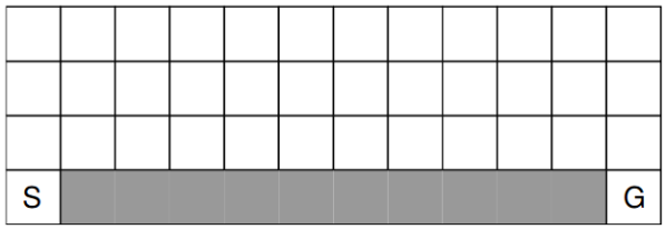
The Cliff Walking experiment as shown in Figure 2 is a classic scenario proposed in Sutton and Barto (2018) and used frequently ever since (e.g., van Seijen et al. (2009)). The agent needs to get from the start state [S] to the goal state [G], while avoiding stepping into the cliff, otherwise rendering a reward of $-100$ and sending him back to the start. For every move which does not lead into the cliff the agent receives a reward of $-1$.

Figure 2. The Cliff Walking: The agent needs to get from the start [S] to the goal [G], avoiding the cliff (grey tiles).

Puddle World: multi-agent

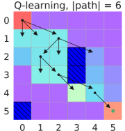
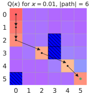
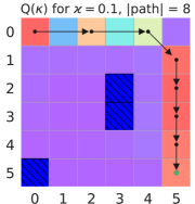
The Puddle World environment is a grid world with puddles which need to be avoided by the joint-action learning agents. The two agents jointly control the movement of a single robot in the Puddle World, each controlling either direction $\langle\text{up},\text{down}\rangle$ or $\langle\text{left},\text{right}\rangle$. Agent 1 can take the actions {stay, move down, move up} and agent 2 can choose {stay, move left, move right, move right by 2}, thus their action spaces are different, further complicating the learning process compared to the single-agent scenario. The joint action is the combination of the two selected actions. We assume a reward of -1 for every move and -100 for stepping into a puddle (returning to the start node). The agents have to move together from the start node at the top left corner to the goal at the bottom right corner. Figure 3 shows the policy learned by our proposed algorithm Q($\kappa$) for the two joint-learning agents. Note how a safer path (longer, avoiding the puddles) is learned with increasing parameter $\varkappa$ (i.e., higher probability of SREs). For $\varkappa=0$ our algorithm degenerates to Q-learning (left panel).

Figure 3. The Puddle World: Q($\kappa$) learns a safer path with increasing $\varkappa$. Puddles are dark blue, the arrows show the optimal actions on the learned path, and the heatmap shows the number of visits to each state (, blue is none).

6.1. Performance

We replicate the experiment of van Seijen et al. (2009) on the Cliff Walking domain, in which we compare our $\kappa$ methods with Q-learning, SARSA and Expected SARSA, and perform a similar experiment on the Puddle World domain. In line with (van Seijen et al., 2009) we show (i) early performance, which is the average return over the first $100$ training episodes, and (ii) converged performance, which is the average return over $100,000$ episodes.

Figure 4. The Cliff Walking (single-agent) in first row and the Puddle World (multi-agent) in second row. Deterministic environment (first column), 10 % stochastic environment (second column) and 10 % attack while training (third column). $\epsilon$-greedy policy with fixed $\epsilon=0.1$. Early performance - dashed lines ($100$ episodes), converged performance - solid lines ($100,000$ episodes).

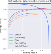
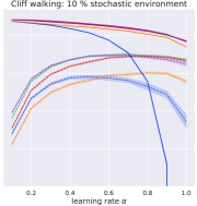
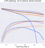
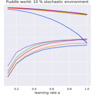
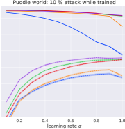
Figure 4 shows the results for three different settings of both scenarios: (i) a deterministic environment, where each action chosen by the policy is executed with certainty; (ii) an environment with $10\%$ stochasticity, in which a random action is taken with $10\%$ of the time; and (iii) an environment with $10\%$ probability of attack, in which an adversarial action is taken $10\%$ of the time. As before, we define an attack as an action that minimizes the Q-value in the given state. The stochastic environment can be seen as modelling random failures.

The early performance experiments are averaged over 300 trials and the converged performance experiments are averaged over 10 trials. We also show the $95\%$ confidence intervals on all results. We fix the exploration rate to $\epsilon=0.1$; for the $\kappa$ methods we set $\varkappa=0.1$ (later in this section we also experiment with different settings of $\varkappa$). Note that the y-axis, showing the average return, is the same in each row for easy comparison. The x-axis shows different learning rates $\alpha$. We can see how the average return decreases with more complex scenarios, from deterministic, over to stochastic, to one with attacks. The $\kappa$ methods are superior to the other baselines in the early performance experiments, especially in the attack case, which is the scenario the $\kappa$ methods are designed for. In the converged performance experiments the $\kappa$ methods beat Q-learning and SARSA and performs at least as well as Expected SARSA.

6.2. Different Levels of Probability of Attack

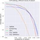
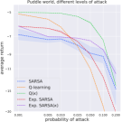
In this section we investigate how the methods behave under different levels of attack, defined by the probability of attack per state. We consider an attack on trained (converged) methods, thus we first train each method for $100,000$ episodes (in deterministic environment) and then we test it on $50,000$ trials with given probability of attack per state. We average the results over $10$ trials and provide $95\%$ confidence intervals. Note, that this is a different methodology of testing the methods against an adversarial attack compared to the experiments in Figure 4, where we considered attacks during training. This experiment shows the strength of the $\kappa$ methods for different levels of attacks. We assume the probability of attack to be known here and thus we set the parameter $\varkappa$ to be equal to that probability, which is the meaning of the parameter $\varkappa$ as described before. In other words, parameter $\varkappa$ prescribes how much safely we want to act. We consider very rare attacks ($0.001$ probability of attack in each state) to more frequent attacks ($0.2$ probability of attack in each state) as shown in Figure 5. For better visualisation we use logarithmic axes. We train all the methods with fixed exploration rate $\epsilon=0.1$ and learning rate $\alpha=0.1$, note that the methods (except SARSA) converge to the same result for different learning rates as shown in left panel of Figure 4. SARSA is very unstable for different learning rates (demonstrated by wide confidence intervals), learns different paths for different $\alpha$ and does not converge fast enough or not at all, which can be partly explained by its higher variance van Seijen et al. (2009). We test the different levels of probability of attack on the Cliff Walking experiment in the left panel of Figure 5, where we can see that the $\kappa$ methods compare favourably to the other baselines, however in some parts they give similar performance as Expected SARSA or SARSA. The Cliff Walking experiment has a limited expressiveness for testing the methods due to a limited number of possible safe paths with low costs (see Figure 2), which is the reason for the $\kappa$ methods to show only similar performance compared to the baselines, not reaching their full potential. However, the Puddle World is more expressive, because there are several possible paths differing in level of safety and cost. The bigger solution space of the Puddle World is also induced by the two cooperating agents, each having their own action space. Therefore, on the right panel of Figure 5 we show the Puddle World experiment for different levels of probability of attack. Here, we can clearly see the $\kappa$ methods outperform the baselines, especially Q($\kappa$) is superior over the whole range of considered probabilities of attack. Note that Q($\kappa$) learns a safer path even for very rare attacks ($0.001$), which is also shown in Figure 3, where Q($\kappa$) learns a path with the same cost (distance) compared to Q-learning, but further to the puddles.

Figure 5. Varying probability of attack: Cliff Walking (left), Puddle World (right), trained 100k, test 50k, $\alpha=0.1$, $\epsilon=0.1$.

6.3. Robustness Analysis

We now test the robustness of the proposed algorithms to an incorrect attack model, meaning that the value of $\varkappa$ in Q($\kappa$) and Expected SARSA($\kappa$) no longer matches the actual probability of attack (in our previous experiments $\varkappa$ matched the actual probability of attack precisely). Figure 6 shows the performance of our algorithms for a range of actual attack probabilities (y-axis) while learning using a fixed parameter $\varkappa=0.1$.

Figure 6. Robustness analysis: Cliff Walking (left), Puddle World (right), trained 100k, test 50k, $\alpha=0.1$, $\epsilon=0.1$, $\varkappa=0.1$.

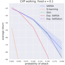
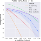
To better highlight the robustness of our methods we choose a range of relatively high actual probabilities of attack around the fixed value of $\varkappa=0.1$ (note that we no longer use a logarithmic scale). One can see that even when $\varkappa$ is not equal to the actual probability of attack the proposed $\kappa$ algorithms still outperform the baselines in most cases. In the Cliff Walking experiment (Figure 6 left) the $\kappa$ methods perform similar to SARSA, however SARSA is quite unstable, as discussed before and as one can see by the width of the confidence interval. The Puddle World experiment (Figure 6 right) demonstrates the superior performance of the $\kappa$ methods, which beat all the baselines even for the fixed parameter $\varkappa$. These results show that even when we do not know the probability of attack accurately we can learn a more robust strategy using the $\kappa$ methods.

7. Discussion and Conclusion

We presented a new operator $\kappa$ for temporal difference learning, which improves robustness of the learning process against potential attacks or perturbations in control. We proved convergence of Q($\kappa$) and Expected SARSA($\kappa$) to (i) the optimal value function $Q^{\star}$ of the original MDP in the limit where $\varkappa\rightarrow 0$; and (ii) the optimal robust value function $Q^{\star}_{\kappa}$ of the MDP that is generalized w.r.t. $\kappa$ for constant parameter $\varkappa$, in both single- and multi-agent versions of the methods. Our complementary empirical results demonstrated that the proposed $\kappa$-methods indeed provide robustness against a chosen scenario of potential attacks and failures. Although our method assumes that a model of such attacks and failures is known to the agent, we further demonstrated that our methods are robust against small model errors. Moreover, we have shown that even in absence of attacks or failures, our method learns a policy that is robust in general against environment stochasticity, in particular in the early stages of learning.

There are several interesting directions for future work. The control space can be extended, allowing for more agents being attacked or malfunctioning with different intensity, or with control transitions depending on additional variables other than the state. Furthermore, the target of adversarial policies could be learned from experience using ideas from opponent modelling (e.g. DPIQN Hong et al. (2018)). Our proposed operator $\kappa$ can potentially be combined with some recent state-of-the-art reinforcement learning methods. For example, the operator could be combined with the multi-step Retrace($\lambda$) (Munos et al., 2016) algorithm, potentially speeding up convergence. Mixed multi-step updates could be introduced by combination with Q($\sigma$) (Asis et al., 2018), where the parameter $\sigma$ can also be state-dependent similarly to the control transitions in our model, allowing to learn robust policies against e.g. multi-step attacks. Another interesting extension along this line would be to model the control transition similar to the options framework (Sutton et al., 1999; Bacon et al., 2017), in which case the alternate control policies could be seen as “malicious” options over which the agent has no control, with potentially complex initiation sets and termination conditions. Such extensions would further increase the flexibility of our proposed operator and narrow the reality gap, making it applicable to a wide range of real-world scenarios.

This project has received funding in the framework of the joint programming initiative ERA-Net Smart Energy Systems’ focus initiative Smart Grids Plus, with support from the European Union’s Horizon 2020 research and innovation programme under grant agreement No 646039. We are indebted to the anonymous reviewers of AAMAS 2019 for their valuable feedback.

References

- (1)
- Asis et al. (2018) Kristopher De Asis, J. Hernandez-Garcia, G. Holland, and Richard S. Sutton. 2018. Multi-Step Reinforcement Learning: A Unifying Algorithm. In AAAI Conference on Artificial Intelligence.
- Bacon et al. (2017) Pierre-Luc Bacon, Jean Harb, and Doina Precup. 2017. The Option-Critic Architecture. In Proceedings of Association for the Advancement of Artificial Intelligence Conference (AAAI). 1726–1734.
- Ciosek and Whiteson (2017) Kamil Andrzej Ciosek and Shimon Whiteson. 2017. OFFER: Off-Environment Reinforcement Learning. In Proceedings of Association for the Advancement of Artificial Intelligence Conference (AAAI).
- Claus and Boutilier (1998) Caroline Claus and Craig Boutilier. 1998. The dynamics of reinforcement learning in cooperative multiagent systems. AAAI/IAAI (1998), 746–752.
- Cristian et al. (1996) Flaviu Cristian, Bob Dancey, and Jon Dehn. 1996. Fault-tolerance in air traffic control systems. ACM Transactions on Computer Systems (TOCS) 14, 3 (1996), 265–286.
- Dvoretzky (1956) Aryeh Dvoretzky. 1956. On Stochastic Approximation. In Proceedings of the Third Berkeley Symposium on Mathematical Statistics and Probability, Volume 1: Contributions to the Theory of Statistics. University of California Press, 39–55.
- Foerster et al. (2018) Jakob N Foerster, Gregory Farquhar, Triantafyllos Afouras, Nantas Nardelli, and Shimon Whiteson. 2018. Counterfactual multi-agent policy gradients. In Thirty-Second AAAI Conference on Artificial Intelligence.
- Garcıa and Fernández (2015) Javier Garcıa and Fernando Fernández. 2015. A comprehensive survey on safe reinforcement learning. Journal of Machine Learning Research 16, 1 (2015), 1437–1480.
- Gaskett (2003) Chris Gaskett. 2003. Reinforcement learning under circumstances beyond its control. In Proceedings of the International Conference on Computational Intelligence for Modelling Control and Automation.
- Hong et al. (2018) Zhang-Wei Hong, Shih-Yang Su, Tzu-Yun Shann, Yi-Hsiang Chang, and Chun-Yi Lee. 2018. A deep policy inference q-network for multi-agent systems. In Proceedings of the 17th International Conference on Autonomous Agents and MultiAgent Systems. 1388–1396.
- Jaakkola et al. (1994) Tommi Jaakkola, Michael I Jordan, and Satinder P Singh. 1994. Convergence of stochastic iterative dynamic programming algorithms. In Advances in Neural Information Processing Systems. 703–710.
- Klima et al. (2016) Richard Klima, Karl Tuyls, and Frans Oliehoek. 2016. Markov Security Games: Learning in Spatial Security Problems. NIPS Workshop on Learning, Inference and Control of Multi-Agent Systems (2016), 1–8.
- Knight (2002) John C Knight. 2002. Safety critical systems: challenges and directions. In Proceedings of the 24th International Conference on Software Engineering. ACM, 547–550.
- Korzhyk et al. (2011) Dmytro Korzhyk, Zhengyu Yin, Christopher Kiekintveld, Vincent Conitzer, and Milind Tambe. 2011. Stackelberg vs. Nash in Security Games: An Extended Investigation of Interchangeability, Equivalence, and Uniqueness. Journal of Artificial Intelligence Research 41 (2011), 297–327.
- Littman (1994) Michael L. Littman. 1994. Markov games as a framework for multi-agent reinforcement learning. Technical Report. Brown University. 157–163 pages.
- Liu et al. (2012) Jing Liu, Yang Xiao, Shuhui Li, Wei Liang, and CL Philip Chen. 2012. Cyber security and privacy issues in smart grids. IEEE Communications Surveys & Tutorials 14, 4 (2012), 981–997.
- Lou et al. (2017) Jian Lou, Andrew M Smith, and Yevgeniy Vorobeychik. 2017. Multidefender security games. IEEE Intelligent Systems 32, 1 (2017), 50–60.
- Morimoto and Doya (2005) Jun Morimoto and Kenji Doya. 2005. Robust reinforcement learning. Neural computation 17, 2 (2005), 335–359.
- Munos et al. (2016) Rémi Munos, Tom Stepleton, Anna Harutyunyan, and Marc Bellemare. 2016. Safe and efficient off-policy reinforcement learning. In Advances in Neural Information Processing Systems (NIPS). 1054–1062.
- Pita et al. (2008) James Pita, Manish Jain, Janusz Marecki, Fernando Ordonez, Christopher Portway, Milind Tambe, Craig Western, Praveen Paruchuri, and Sarit Kraus. 2008. Deployed ARMOR Protection: The Application of a Game Theoretic Model for Security at the Los Angeles International Airport. In International Joint Conference on Autonomous Agents and Multiagent Systems (AAMAS), Vol. 3. 1805–1812.
- Robbins and Monro (1951) Herbert Robbins and Sutton Monro. 1951. A Stochastic Approximation Method. The Annals of Mathematical Statistics 22, 3 (1951), 400–407.
- Ruan et al. (2005) Sui Ruan, Candra Meirina, Feili Yu, Krishna R Pattipati, and Robert L Popp. 2005. Patrolling in a stochastic environment. Technical Report. Electrical and Computer Engineering Department, University of Connecticut, Storrs.
- Shieh et al. (2012) Eric Shieh, Bo An, Rong Yang, Milind Tambe, Craig Baldwin, Joseph DiRenzo, Ben Maule, and Garrett Meyer. 2012. PROTECT: A Deployed Game Theoretic System to Protect the Ports of the United States. International Conference on Autonomous Agents and Multiagent Systems (AAMAS) 1 (2012), 13–20.
- Shooman (2003) Martin L Shooman. 2003. Reliability of computer systems and networks: fault tolerance, analysis, and design. John Wiley & Sons.
- Singh et al. (2000) Satinder Singh, Tommi Jaakkola, Michael L Littman, and Csaba Szepesvári. 2000. Convergence results for single-step on-policy reinforcement-learning algorithms. Machine learning 38, 3 (2000), 287–308.
- Singh et al. (1994) Satinder P Singh, Andrew G Barto, Roderic Grupen, and Christopher Connolly. 1994. Robust reinforcement learning in motion planning. In Advances in Neural Information Processing Systems (NIPS). 655–662.
- Smart (1974) D. R. Smart. 1974. Fixed point theorems. Cambridge University Press, Cambridge.
- Sunehag et al. (2017) Peter Sunehag, Guy Lever, Audrunas Gruslys, Wojciech Marian Czarnecki, Vinicius Zambaldi, Max Jaderberg, Marc Lanctot, Nicolas Sonnerat, Joel Z Leibo, Karl Tuyls, and Thore Grapel. 2017. Value-decomposition networks for cooperative multi-agent learning. arXiv preprint arXiv:1706.05296 (2017).
- Sutton and Barto (2018) Richard S. Sutton and Andrew G. Barto. 2018. Reinforcement Learning: An Introduction (second ed.). The MIT Press, Cambridge, MA.
- Sutton et al. (1999) Richard S Sutton, Doina Precup, and Satinder Singh. 1999. Between MDPs and semi-MDPs: A framework for temporal abstraction in reinforcement learning. Artificial Intelligence 112, 1-2 (1999), 181–211.
- Szepesvari and Littman (1997) Csaba Szepesvari and Michael L Littman. 1997. Generalized Markov Decision Processes: Dynamic-programming and Reinforcement-learning Algorithms. Technical Report. Brown University.
- Tsitsiklis (1994) John N Tsitsiklis. 1994. Asynchronous stochastic approximation and Q-learning. Machine Learning 16, 3 (1994), 185–202.
- van Seijen et al. (2009) Harm van Seijen, Hado van Hasselt, Shimon Whiteson, and Marco Wiering. 2009. A theoretical and empirical analysis of Expected Sarsa. In IEEE Symposium on Adaptive Dynamic Programming and Reinforcement Learning, ADPRL 2009. 177–184.
- Yan et al. (2013) Ye Yan, Yi Qian, Hamid Sharif, and David Tipper. 2013. A survey on smart grid communication infrastructures: Motivations, requirements and challenges. IEEE Communications Surveys & Tutorials 15, 1 (2013), 5–20.
- Zhou and Doyle (1998) Kemin Zhou and John Comstock Doyle. 1998. Essentials of robust control. Vol. 104. Prentice hall, Upper Saddle River, NJ.