Multi-kink scattering in the double sine-Gordon model

Abstract

We study collisions of two, three, and four kinks of the double sine-Gordon model. The initial conditions are taken in a special form in order to provide collision of all kinks in one point. We obtain dependences of the maximal energy densities on the model parameter. We also analyze the final states observed in these collisions.

I Introduction

Interactions of kinks — solutions of the type of solitary waves of non-integrable field-theoretical models in (1+1)-dimensional space-time — are of growing interest Rajaraman.book.1982 ; Vilenkin.book.2000 ; Manton.book.2004 ; Vachaspati.book.2006 . Great amount of important results has been obtained recently for the kink-(anti)kink scattering Gani.PRD.2014 ; Gani.JHEP.2015 ; Gani.JPCS.2016.phi8 ; Bazeia.EPJC.2018.sinh ; Bazeia.JPCS.2017.sinh ; Gani.EPJC.2018.dsg ; Belendryasova.JPCS.2019.dsg ; Gomes.JHEP.2018 ; Bazeia.2018.hybrid ; Dorey.PLB.2018.quasinormal ; Campos.2019.quasinormal ; Zhong.2019.inner . In many cases rather non-trivial picture of interaction has been observed. In particular, it was found that the collision of kink and antikink crucially depends on the initial velocity $v_{\mathrm{in}}$ (in the numerical experiments kink and antikink are initially placed at large distance from each other and are moving towards each other with the initial velocities $v_{\mathrm{in}}$ in the laboratory frame of reference). There is a critical value of the initial velocity $v_{\mathrm{cr}}$, which separates two different regimes of the collision. At $v_{\mathrm{in}}>v_{\mathrm{cr}}$ inelastic reflection of kinks (or passing through each other, if the model allows such process) is observed. At $v_{\mathrm{in}}<v_{\mathrm{cr}}$ after the collision the kink and antikink form a long-living bound state — a bion — which decays slowly radiating energy in the form of small-amplitude waves. Besides, in some models at $v_{\mathrm{in}}<v_{\mathrm{cr}}$ an interesting phenomenon was found — so-called escape windows. Escape windows are intervals of the initial velocity, at which kinks do not form a bion, but escape from each other after two or more collisions. The cause of this phenomenon is the resonance energy exchange between translational and vibrational modes of the kink (antikink), see, e.g., Refs. Campbell.PhysD.1986 ; Kudryavtsev.UFN.1997.eng ; Kudryavtsev.UFN.1997.rus . In some models the kinetic energy of the kinks can be stored in vibrational modes of the system “kink+antikink” Gani.PRE.1999 ; Dorey.PRL.2011 ; Belendryasova.CNSNS.2019.phi8 ; Belendryasova.JPCS.2017.phi8 .

Another very interesting subject that should be mentioned here is interactions of kinks having power-law tails, see, e.g., Refs. Belendryasova.CNSNS.2019.phi8 ; Belendryasova.JPCS.2017.phi8 ; Gomes.PRD.2012 ; Radomskiy.JPCS.2017.tails ; Christov.PRD.2019.long-range ; Christov.2018.long-tails ; Manton.2018.long-range ; Manton.JPA.2018.long-range ; Bazeia.JPC.2018.polynomial-tails . Such kinks arise in various models with both polynomial and non-polynomial potentials. The power-law asymptotics (“fat tails”) of kinks result in their long-range interaction, i.e. the kinks feel each other at very large distances. As a result, the traditionally used initial conditions in the form of superposition of kink and antikink seem to be not valid for simulation of the kink-antikink scattering Christov.PRD.2019.long-range .

The interactions of kinks are studied both numerically and analytically. On the one hand, the scattering processes can be simulated directly by using the numerical methods of solving equations of motion – partial differential equations of second order. On the other hand, there are analytical approximate methods which allow to estimate forces between kink and (anti)kink. These are (i) the collective coordinate approximation Gani.PRD.2014 ; Weigel.PRD.2016.cc ; Demirkaya.JHEP.2107.cc and (ii) Manton’s method (Manton.book.2004, , Ch. 5), Perring.NuclPhys.1962 ; Rajaraman.PRD.1977 ; Manton.NPB.1979 ; Kevrekidis.PRE.2004 .

It is worth to mention that kink-like solutions can also be obtained in more complicated models with two or more scalar fields GaKu.SuSy.2001.eng ; GaKu.SuSy.2001.rus ; Lensky.JETP.2001.eng ; Lensky.JETP.2001.rus ; Alonso-Izquierdo.PRD.2002 ; Kurochkin.CMMP.2004.eng ; Kurochkin.CMMP.2004.rus ; Alonso-Izquierdo.AHEP.2013.kink-like ; Alonso-Izquierdo.JHEP.2014.moduli ; Katsura.PRD.2014 ; Alonso-Izquierdo.Physica_D.2018.dynamics ; Alonso-Izquierdo.PRD.2018.collisions ; Alonso-Izquierdo.2018.MSTB ; Alonso-Izquierdo.2019.scattering ; Morris.AP.2018.mixing ; Alonso-Izquierdo.2019.non-topological ; Mohammadi.CNSNS.2019.two-field-sg . In particular, in GaKu.SuSy.2001.eng ; GaKu.SuSy.2001.rus ; Alonso-Izquierdo.PRD.2002 ; Alonso-Izquierdo.Physica_D.2018.dynamics ; Alonso-Izquierdo.PRD.2018.collisions ; Alonso-Izquierdo.2018.MSTB ; Alonso-Izquierdo.2019.scattering ; Morris.AP.2018.mixing ; Alonso-Izquierdo.2019.non-topological the models with two real scalar fields with polynomial potentials have been studied. In GaLiRa ; GaLiRaconf ; blyankinshtein ; GaKsKu01.eng ; GaKsKu01.rus ; GaKsKu02.eng ; GaKsKu02.rus configurations of the type of domain wall with additional fields localized on it were investigated. Many important results have also been obtained for non-topological field configurations — lumps, Q-balls, etc. Brihaye.PRD.2015 ; Loginov.YadFiz.2011.eng ; Loginov.YadFiz.2011.rus ; Bazeia.EPJC.2017 ; Bazeia.fermion.2017 ; Schweitzer.PRD.2012.1 ; Schweitzer.PRD.2012.2 ; Schweitzer.NPA.2016 ; Nugaev.PRD.2013 ; Bazeia.EPJC.2016.Q-balls ; Bazeia.PLB.2016.Q-balls ; Bazeia.PLB.2017.Q-balls ; Levkov.JHEP.2017.Q-balls ; Loiko.PRD.2018.Q-balls ; Kovtun.PRD.2018.Q-balls ; Loginov.PLB.2018.Q-balls ; Loginov.arXiv.2019.Q-balls .

Kinks, domain walls and other topological defects arise in a great amount of models, hence they are very important for various physical applications from condensed matter to high energy physics and cosmology poltis1 ; valle2016 ; Matsui.JCAP.2016 ; Wachter.PRL.2017 ; Ye.EPJC.2017 ; Ringeval.JCAP.2017 ; GaKiRu ; GaKiRu.conf , see also Vilenkin.book.2000 . Many physical phenomena could be effectively described by one-dimensional topological structures. For example, a three-dimensional domain wall in the direction perpendicular to it can be viewed as a one-dimensional topological field configuration — kink connecting two different vacua of the model. At the same time, the case of $(1+1)$-dimensional space-time structure can be investigated more easily compared to $2+1$ or $3+1$ dimensions.

The processes of collision of several kinks in one point (with extracting maximal energy densities) have been actively investigated over the last few years saadatmand.prd.2015 ; Moradi.JHEP.2017.multikink ; Moradi.EPJB.2017.multikink ; Moradi.CNSNS.2017.multikink ; saad.WaveMotion.2018 . Such processes are of interest for numerous applications. Being topological defects, the kinks bear significant amount of energy. As a result, simultaneous collision of several kinks (antikinks) in one point can lead to formation of spatial domains with high energy density. The authors of Ref. saad.WaveMotion.2018 have shown that with knowing maximal energy densities in collision of $N$ kinks one can predict how many kink-antikink pairs can be produced in particle collisions.

This study deals with the collisions of several kinks of the double sine-Gordon (DSG) model in one point. This model has been actively studied due to its numerous applications, see, e.g., Gani.EPJC.2018.dsg ; Gani.PRE.1999 ; Campbell.PhysD.1986.dsg ; Malomed.PLA.1989.dsg ; Nazifkar.BJP.2010.dsg and references therein. Note that the subject of multi-kink collisions is very vast. The number of parameters that could be changed is very large. These are, in particular, the model parameter $R$, the initial velocities and the initial positions of kinks. In this paper we study collisions of two three and four kinks in one point (in a small spatial region). We focus on the dependences of maximal energy densities on the model parameter $R$. In collisions of four kinks (two kinks and two antikinks, to be more accurate) we investigate how the final configurations depend on $R$. In our numerical simulations we use fixed initial positions and initial velocities of kinks.

Our paper is organized as follows. In Sect. II we recall the main features of the DSG model, write down its kinks, and discuss their main properties. Section III presents the results of the numerical simulations of multi-kink collisions. We conclude with summarizing in Sect. IV, where we also formulate some possible directions for further research.

II Double sine-Gordon model

Within the $(1+1)$-dimensional double sine-Gordon model the dynamics of the real scalar field $\phi(x,t)$ is described by the Lagrangian density

$$\mathcal{L}=\frac{1}{2}\left(\frac{\partial\phi}{\partial t}\right)^{2}-\frac{1}{2}\left(\frac{\partial\phi}{\partial x}\right)^{2}-V(\phi),$$ (1)

where the potential $V(\phi)$ is non-negative function of the field. From the Lagrangian (1) one can obtain the equation of motion for the field $\phi(x,t)$:

$$\frac{\partial^{2}\phi}{\partial t^{2}}-\frac{\partial^{2}\phi}{\partial x^{2}}+\frac{dV}{d\phi}=0.$$ (2)

Below we simulate multi-kink scattering by solving this equation numerically.

In literature there are various modifications and parameterizations of the potential, which all can be called “double sine-Gordon potential”. We will use the so-called $R$-parameterization, see, e.g., Refs. Gani.EPJC.2018.dsg ; Gani.PRE.1999 ; Campbell.PhysD.1986.dsg . In this parameterization the DSG potential is:

$$V(\phi)=\tanh^{2}R\>(1-\cos\phi)+\frac{4}{\cosh^{2}R}\left(1+\cos\frac{\phi}{2}\right).$$ (3)

In Fig. 1 we show (a) this potential for some values of the parameter and (b) the $R$-dependence of the coefficients in front of $(1-\cos\phi)$ and $\displaystyle\left(1+\cos\frac{\phi}{2}\right)$, which are responsible for the “mixing” of $\phi$– and $\displaystyle\frac{\phi}{2}$–sine-Gordon potentials.

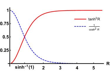
(a)

Figure 1: (a) Potential of the DSG model; (b) $R$-dependence of the coefficients in the potential, which are responsible for the mixing of two sine-Gordon potentials.

Depending on $R$, the potential (3) looks different. In particular,

$$V(\phi)=\begin{cases}4\left(1+\cos\displaystyle\frac{\phi}{2}\right)\quad\mbox{for}\quad R=0,\\ 4-\left(1-\cos\displaystyle\frac{\phi}{2}\right)^{2}\quad\mbox{for}\quad R=\mbox{arsinh}\>1,\\ 1-\cos\phi\quad\mbox{for}\quad R\to+\infty.\end{cases}$$ (4)

The double sine-Gordon model has static topological solution — kink (antikink):

$$\phi_{\mathrm{k}(\mathrm{\bar{k}})}(x)=4\pi n\pm 4\arctan\frac{\sinh x}{\cosh R}.$$ (5)

Notice that for better understanding of many processes in kinks collisions the following fact could be important: the DSG kink (antikink) (5) can be interpreted as a superposition of two sine-Gordon solitons:

$$\phi_{\mathrm{k}(\mathrm{\bar{k}})}(x)=4\pi n\pm\left[\phi_{\mathrm{SGK}}(x+R)-\phi_{\mathrm{SGK}}(R-x)\right],$$ (6)

where

$$\phi_{\mathrm{SGK}}(x)=4\arctan\exp(x)$$ (7)

is the sine-Gordon kink (soliton). Thus the DSG kink can be viewed as a superposition of two sine-Gordon kinks, which are separated by the distance $2R$ (if the DSG kink is centered at $x=0$ then the two sine-Gordon solitons are centered at $x=\pm R$), see Fig. 2.

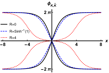
Figure 2: Kinks (monotonously increasing functions $\phi_{\mathrm{k}}(x)$) and antikinks (monotonously decreasing functions $\phi_{\mathrm{\bar{k}}}(x)$) of the DSG model for three different values of the parameter $R$.

Due to the Lorentz invariance, the kink (antikink) moving along the $x$-axis with the velocity $v$ can be obtained by the Lorentz boost:

$$\phi_{\mathrm{k}(\mathrm{\bar{k}})}(x,t)=\phi_{\mathrm{k}(\mathrm{\bar{k}})}(\gamma(x-vt)),$$ (8)

where $\gamma=1/\sqrt{1-v^{2}}$ is the Lorentz factor.

The energy functional which corresponds to the Lagrangian (1) reads

$$E[\phi]=\int\limits_{-\infty}^{\infty}\left[\frac{1}{2}\left(\frac{\partial\phi}{\partial t}\right)^{2}+\frac{1}{2}\left(\frac{\partial\phi}{\partial x}\right)^{2}+V(\phi)\right]dx.$$ (9)

The total energy (9) can be split into three parts: (i) the kinetic energy $K$, (ii) the gradient energy $U$, and (iii) the potential energy $P$:

$$E=K+U+P.$$ (10)

According to this, the integrand in (9), i.e. the total energy density $\varepsilon(x,t)$, can be written as

$$\varepsilon(x,t)=k(x,t)+u(x,t)+p(x,t),$$ (11)

where

$$k(x,t)=\frac{1}{2}\left(\frac{\partial\phi}{\partial t}\right)^{2},\quad u(x,t)=\frac{1}{2}\left(\frac{\partial\phi}{\partial x}\right)^{2},\quad p(x,t)=V(\phi)$$ (12)

are (i) the kinetic energy density, (ii) the gradient energy density, and (iii) the potential energy density, respectively.

In the case of one moving kink $\phi_{\mathrm{k}}(x,t)$ we have:

$$p(x,t)=\frac{8\cosh^{2}R\cdot\cosh^{2}[\gamma(x-vt)]}{\left(\cosh^{2}R+\sinh^{2}[\gamma(x-vt)]\right)^{2}}=(1-v^{2})\,u(x,t)=\frac{1-v^{2}}{v^{2}}\,k(x,t)=\frac{1-v^{2}}{2}\,\varepsilon(x,t).$$ (13)

Integrating the total energy density with respect to $x$, we obtain the total energy of the moving kink:

$$E_{\mathrm{K}}=\int_{-\infty}^{+\infty}\varepsilon(x,t)\>dx=\frac{M_{\mathrm{K}}}{\sqrt{1-v^{2}}},$$ (14)

where

$$M_{\mathrm{K}}=16\left(1+\frac{2R}{\sinh 2R}\right)$$ (15)

is the mass of kink, i.e. the energy of the static DSG kink.

In the next section we present the results of the numerical simulation of collisions of two, three and four DSG kinks in the same point. We find the maximal (over the spatial coordinate $x$ and time $t$) values of the energy densities mentioned above: kinetic, gradient, potential and total. Note that for one moving kink the maximal values can be obtained analytically. Depending on the parameter $R$, they are the following:

$$p_{\mathrm{max}}^{(1)}=(1-v^{2})\,u_{\mathrm{max}}^{(1)}=\frac{1-v^{2}}{v^{2}}\,k_{\mathrm{max}}^{(1)}=\frac{1-v^{2}}{2}\,\varepsilon_{\mathrm{max}}^{(1)}=\frac{8}{\cosh^{2}R}$$ (16)

at $R\leq\mbox{arsinh}\,1$, and

$$p_{\mathrm{max}}^{(1)}=(1-v^{2})\,u_{\mathrm{max}}^{(1)}=\frac{1-v^{2}}{v^{2}}\,k_{\mathrm{max}}^{(1)}=\frac{1-v^{2}}{2}\,\varepsilon_{\mathrm{max}}^{(1)}=2\coth^{2}R$$ (17)

at $R\geq\mbox{arsinh}\,1$.

III Multi-kink scattering

We studied the collisions of two kinks (a kink and an antikink), three kinks (two kinks and an antikink), and four kinks (two kinks and two antikinks) at one point. Our main goal was to obtain $R$-dependences of the maximal values of the energy densities — kinetic, gradient, potential and total. To do this, we numerically solved the discretized version of the equation of motion (2),

$$\frac{d^{2}\phi_{n}}{dt^{2}} - \frac{1}{h^{2}}(\phi_{n-1}-2\phi_{n}+\phi_{n+1})+\displaystyle\frac{1}{12h^{2}}(\phi_{n-2}-4\phi_{n-1}+6\phi_{n}-4\phi_{n+1}+\phi_{n+2})$$ (18)

$$+ \tanh^{2}R\>\sin\phi_{n}-\frac{2}{\cosh^{2}R}\sin\frac{\phi_{n}}{2}=0,$$

using Störmer method of integration. Here $h=0.025$ is the space step, $n=0,\pm 1,\pm 2,...$ and $\phi_{n}(t)=\phi(nh,t)$. The second derivative of the field $\phi$ with respect to $x$, $\phi_{xx}$, is discretized with the accuracy $O(h^{4})$. In our numerical experiments we used the range $-375\leq x\leq 375$. Integration with respect to time was performed with the step $\tau=0.005$. We used $0\leq t\leq 500$ for searching maximal energy densities over $x$ and $t$.

The initial conditions for each case (collisions of two, three and four kinks) will be written below. In the case of collisions of three and four kinks, the initial conditions were fit in such a way that the kinks collided in one point.

From the point of view of physical applications, the energy distribution in collision of two or several kinks is of great importance. The point is that a kink is a topological defect, which describes, for example, a planar domain wall or another formation (“defect”) in a real physical system. The kinks collision thus represents mathematical model of collision of such defects, and the energy densities show space-time distribution of energy.

III.1 Kink-antikink scattering

First of all, note that collisions of the DSG kink and antikink have been studied in detail in recent paper Gani.EPJC.2018.dsg . An interesting phenomenon was found — oscillons in the final state. Besides, the dependence of the critical velocity $v_{\mathrm{cr}}$ on $R$ obtained in Gani.EPJC.2018.dsg was somewhat different from that presented in classical paper Campbell.PhysD.1986.dsg . We think that a series of local maxima of the dependence $v_{\mathrm{cr}}(R)$ observed in Gani.EPJC.2018.dsg is a consequence of more detailed investigation of appropriate range of the initial velocities of the colliding kinks.

Unlike the previous works Gani.EPJC.2018.dsg ; Gani.PRE.1999 ; Campbell.PhysD.1986.dsg , we focus on study of maximal energy densities in collisions of the kink and antikink at the initial velocity $v_{\mathrm{in}}=0.1$ and various $R$. To do this we used the initial condition in the form of the kink and antikink, which are initially placed at $x=-x_{0}$ and $x=+x_{0}$ and moving towards each other with the velocities $v=+v_{\mathrm{in}}$ and $v=-v_{\mathrm{in}}$, respectively,

$$\phi_{\mathrm{k}\mathrm{\bar{k}}}(x)=\phi_{\mathrm{k}}\left(\frac{x+x_{0}-v_{\mathrm{in}}t}{\sqrt{1-v_{\mathrm{in}}^{2}}}\right)+\phi_{\mathrm{\bar{k}}}\left(\frac{x-x_{0}+v_{\mathrm{in}}t}{\sqrt{1-v_{\mathrm{in}}^{2}}}\right)-2\pi,$$ (19)

where $\phi_{\mathrm{k}(\mathrm{\bar{k}})}(x)$ is defined by Eq. (5) with $n=0$. This initial configuration is shown in Fig. 3(a).

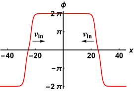
(a)  kink+antikink

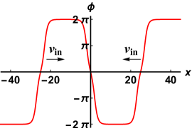
(b)  kink+antikink+kink

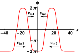
(c)  kink+antikink+kink+antikink

Figure 3: The initial configurations for $R=2$: (a) Eq. (19), (b) Eq. (20), (c) Eq. (21).

In our simulations we used $x_{0}=25$ and $v_{\mathrm{in}}=0.1$. Space-time picture of the collision for some selected values of $R$ is shown in Fig. 4.

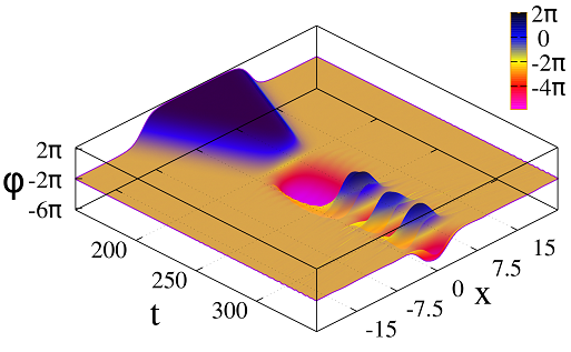
(a)  $R=0.5$

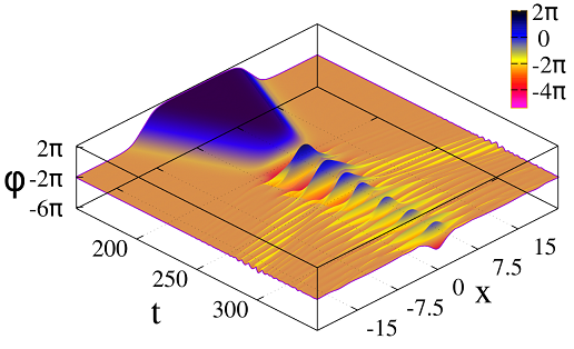
(b)  $R=1.0$

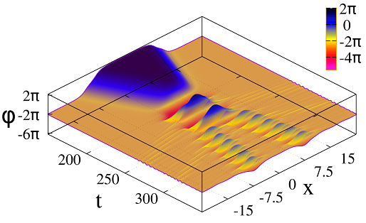
(c)  $R=1.5$

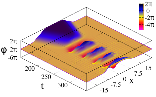
(d)  $R=2.0$

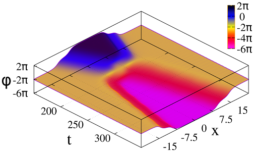
(e)  $R=2.5$

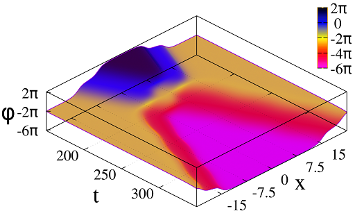
(f)  $R=3.0$

Figure 4: Space-time picture of the kink-antikink collisions for different $R$’s.

We performed numerical simulation of the kink-antikink collisions within a wide range of the parameter $R$. We have obtained the dependences of the maximal energy densities on the parameter $R$, see Fig. 5(d).

(a)  total

(b)  kinetic

(c)  potential

(d)  gradient

Figure 5: Maximal energy densities as functions of $R$ for kink-antikink collisions at $v_{\mathrm{in}}=0.1$

.

These dependences are rather complicated. At $R\stackrel{{\scriptstyle\scriptstyle<}}{{\phantom{}{}_{\sim}}}0.5$ and $R\stackrel{{\scriptstyle\scriptstyle>}}{{\phantom{}{}_{\sim}}}2.5$ we see smooth and monotonously decreasing curves. At the same time, within the range $0.5\stackrel{{\scriptstyle\scriptstyle<}}{{\phantom{}{}_{\sim}}}R\stackrel{{\scriptstyle\scriptstyle<}}{{\phantom{}{}_{\sim}}}2.5$ the dependences look quite stochastic. The observed difference in behavior of the maximal energy densities at various $R$ could be a consequence of different character of kink-antikink interaction at given initial conditions. In particular, depending on the parameter $R$, the initial velocity $v_{\mathrm{in}}=0.1$ can be either less or more than the critical value $v_{\mathrm{cr}}$. The point is that the critical velocity depends on $R$ in a complicated way Gani.EPJC.2018.dsg .

Analyzing the dependence $v_{\mathrm{cr}}(R)$ which is presented in Fig. 6 of Ref. Gani.EPJC.2018.dsg , we can see that the initial velocity $v_{\mathrm{in}}=0.1$ is less than the critical in the range $0.5\stackrel{{\scriptstyle\scriptstyle<}}{{\phantom{}{}_{\sim}}}R\stackrel{{\scriptstyle\scriptstyle<}}{{\phantom{}{}_{\sim}}}2.5$. Thus complicated and almost stochastic behavior of the maximal energy densities is observed for those $R$’s at which the kinks form a bound state, i.e., a bion. On the other hand, at those $R$’s at which the kinks escape from each other after a collision, the smooth and monotonous dependences are observed. We can assume that the complicated dependences of the maximal energy densities on $R$ can be a consequence of complex resonance processes in bion. As a result, energy is redistributed that leads to abrupt changes of the maximal energy densities.

In order to confirm our hypothesis, we performed numerical simulations of the kink-antikink collisions at $v_{\mathrm{in}}=0.17$ and $v_{\mathrm{in}}=0.2$. The maximal energy densities are shown in Figs. 6 and 7. From these figures one can see that regions of the stochastic behavior of the maximal energy densities become narrower. As it was for $v_{\mathrm{in}}=0.1$, at these new initial velocities the stochastic behavior of the energy densities appears at those $R$’s at which $v_{\mathrm{in}}<v_{\mathrm{cr}}(R)$ and the kink and antikink capture each other and form a bion in the final state.

(a)  total

(b)  kinetic

(c)  potential

(d)  gradient

Figure 6: Maximal energy densities as functions of $R$ for kink-antikink collisions at $v_{\mathrm{in}}=0.17$.

(a)  total

(b)  kinetic

(c)  potential

(d)  gradient

Figure 7: Maximal energy densities as functions of $R$ for kink-antikink collisions at $v_{\mathrm{in}}=0.2$.

Another interesting fact is the presence of smooth and monotonous segments of the maximal energy densities in the range $1.5\stackrel{{\scriptstyle\scriptstyle<}}{{\phantom{}{}_{\sim}}}R\stackrel{{\scriptstyle\scriptstyle<}}{{\phantom{}{}_{\sim}}}1.6$, see Fig. 5(d). We can assume that it is a consequence of the fact that at these $R$’s the bound state of kinks evolves differently. The space-time picture of the kink-antikink collision at some selected values of the parameter $R$ from the range $1.49\leq R\leq 1.63$ is shown in Fig. 8. It it clearly seen that at $1.5\stackrel{{\scriptstyle\scriptstyle<}}{{\phantom{}{}_{\sim}}}R\stackrel{{\scriptstyle\scriptstyle<}}{{\phantom{}{}_{\sim}}}1.6$ two escaping oscillons in the final state are formed after two oscillations of the kink-antikink bound state. At other values of $R$ in Fig. 8 the oscillons in the final state are either formed after more complicated evolution of the kink-antikink bound state or not formed at all.

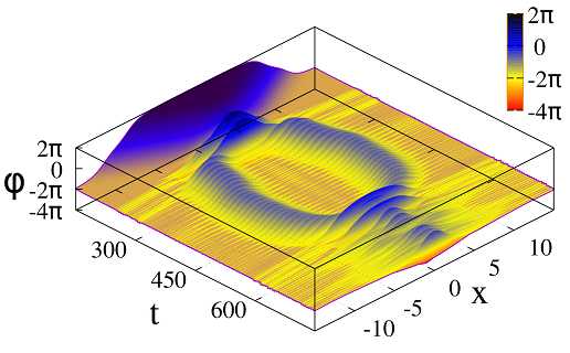
(a)  $R=1.49$

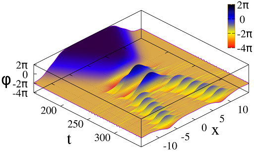
(b)  $R=1.50$

(c)  $R=1.52$

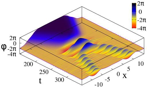
(d)  $R=1.60$

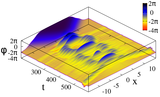
(e)  $R=1.61$

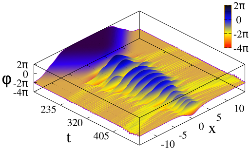
(f)  $R=1.63$

Figure 8: Space-time picture of the kink-antikink collisions for some $R$’s from the range $1.49\leq R\leq 1.63$.

III.2 Collision of two kinks and an antikink

We performed numerical simulation of the collision of three DSG kinks in one point. We used the following initial configuration:

$$\phi_{\mathrm{k\bar{k}k}}(x)=\phi_{\mathrm{k}}\left(\frac{x+x_{0}-v_{\mathrm{in}}t}{\sqrt{1-v_{\mathrm{in}}^{2}}}\right)+\phi_{\mathrm{\bar{k}}}(x)+\phi_{\mathrm{k}}\left(\frac{x-x_{0}+v_{\mathrm{in}}t}{\sqrt{1-v_{\mathrm{in}}^{2}}}\right),$$ (20)

where $\phi_{\mathrm{k}(\mathrm{\bar{k}})}(x)$ is defined by Eq. (5) with $n=0$. This initial condition corresponds to two kinks and an antikink. The antikink is at rest at the origin $x=0$, and two kinks are moving towards the antikink with the initial velocities $v=+v_{\mathrm{in}}$ and $v=-v_{\mathrm{in}}$, starting from $x=-x_{0}$ and $x=+x_{0}$, respectively. This initial configuration is shown in Fig. 3(b). In our simulations we used $x_{0}=25$ and $v_{\mathrm{in}}=0.1$. Space-time picture of the collision for some selected values of $R$ is shown in Fig. 9.

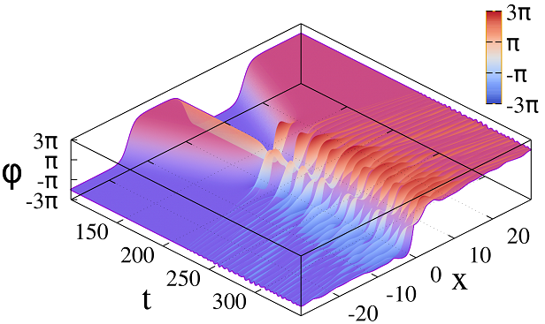
(a)  $R=0.50$

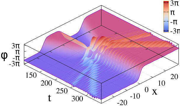
(b)  $R=1.0$

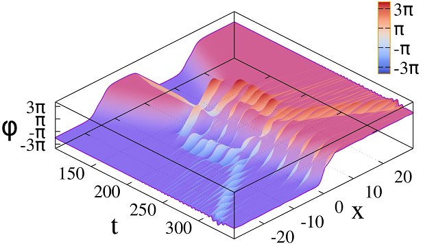
(c)  $R=1.5$

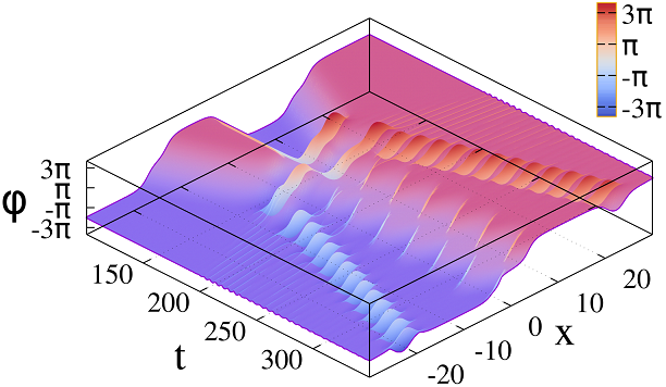
(d)  $R=2.0$

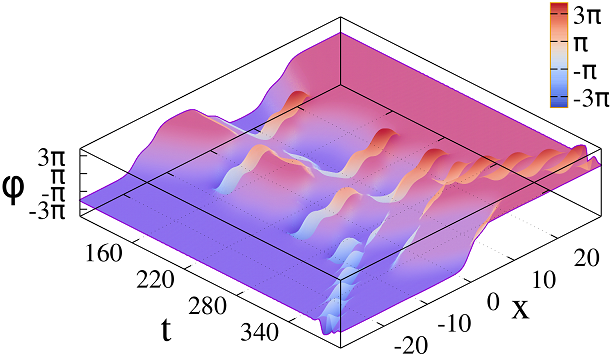
(e)  $R=2.5$

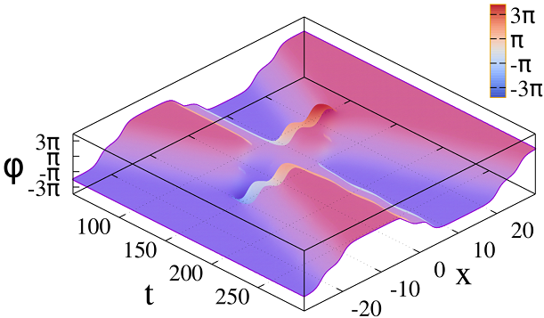
(f)  $R=3.0$

Figure 9: Space-time picture of collisions of three kinks for different $R$’s.

The interaction of three kinks looks rather complicated. In particular, in a pair “kink+antikink” resonance interaction can occur. This leads to appearance of various intermediate and final states, see Fig. 9. (Note that the term “final state” stands here for configuration observed after a long time after the collision. “Long time”, in turn, means a period of time which is much longer than life-times of various bound states (of oscillons, of kink and oscillon, and so on), if such states do not have infinite life-times.)

We have obtained the dependencies of the maximal energy densities on the parameter $R$, see Fig. 10.

(a)  total

(b)  kinetic

(c)  potential

(d)  gradient

Figure 10: Maximal energy densities as functions of $R$ for collisions of three kinks.

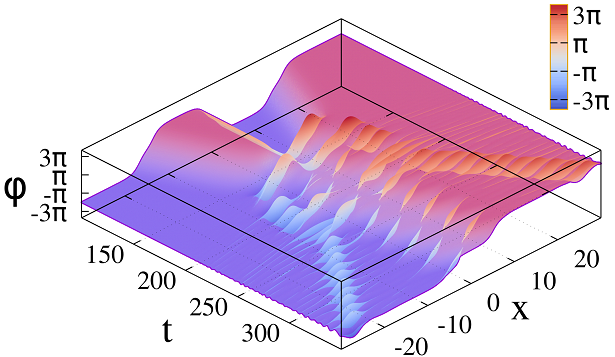
(a)  $R=1.60$

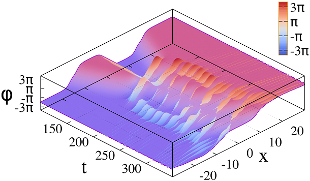
(b)  $R=1.70$

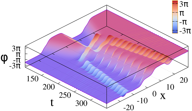
(c)  $R=1.78$

(d)  $R=1.86$

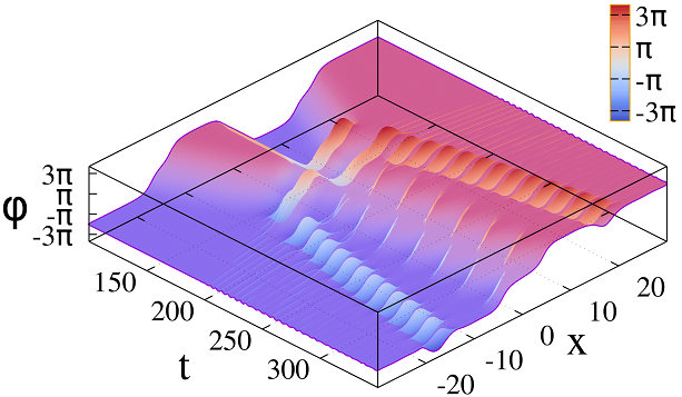
(e)  $R=1.94$

(f)  $R=2.02$

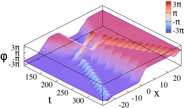
(g)  $R=2.10$

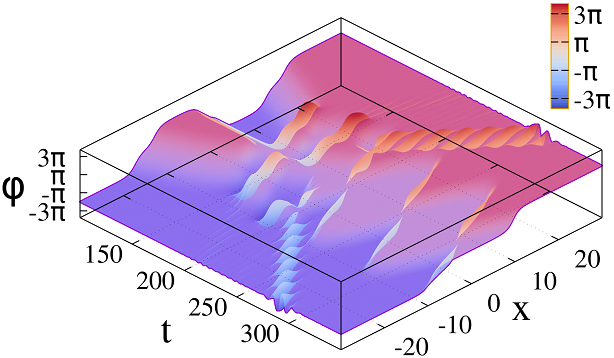
(h)  $R=2.20$

Figure 11: Space-time picture of collisions of three kinks for some $R$’s from the range $1.6\leq R\leq 2.2$.

The maximal potential energy density is monotonously decreasing, while the maximal kinetic, gradient and total energy densities behave in a complicated way, thereby reflecting complex interaction of the three colliding kinks.

Note that in the range $1.7\stackrel{{\scriptstyle\scriptstyle<}}{{\phantom{}{}_{\sim}}}R\stackrel{{\scriptstyle\scriptstyle<}}{{\phantom{}{}_{\sim}}}2.1$ we see a smooth and monotonous segments of the maximal energy densities. We can assume that in this range of $R$ the field evolution is somewhat different. Actually, from Fig. 11 we see that at these $R$’s two escaping oscillons in the final state are formed right after the kinks collision. At the same time, at $R\stackrel{{\scriptstyle\scriptstyle<}}{{\phantom{}{}_{\sim}}}1.7$ and $R\stackrel{{\scriptstyle\scriptstyle>}}{{\phantom{}{}_{\sim}}}2.1$ the escape of oscillons occur after some time during which the oscillons remain bound.

III.3 Collision of two kinks and two antikinks

Finally, we studied the collision of four DSG kinks in one point. To do this, we used the initial configuration of the form of

$$\phi_{\mathrm{k\bar{k}k\bar{k}}}(x)=\phi_{\mathrm{k}}\left(\frac{x+x_{02}-v_{\mathrm{in2}}t}{\sqrt{1-v_{\mathrm{in2}}^{2}}}\right)+\phi_{\mathrm{\bar{k}}}\left(\frac{x+x_{01}-v_{\mathrm{in1}}t}{\sqrt{1-v_{\mathrm{in1}}^{2}}}\right)+$$

$$+\phi_{\mathrm{k}}\left(\frac{x-x_{01}+v_{\mathrm{in1}}t}{\sqrt{1-v_{\mathrm{in1}}^{2}}}\right)+\phi_{\mathrm{\bar{k}}}\left(\frac{x-x_{02}+v_{\mathrm{in2}}t}{\sqrt{1-v_{\mathrm{in2}}^{2}}}\right)-2\pi,$$ (21)

where $\phi_{\mathrm{k}(\mathrm{\bar{k}})}(x)$ is defined by Eq. (5) with $n=0$. The initial configuration (21) corresponds to two kinks and two antikinks moving to the collision point, see Fig. 3(c). We used the following initial values of positions and velocities of the kinks and antikinks: $x_{01}=10$, $x_{02}=25$, $v_{\mathrm{in1}}=0.05$, $v_{\mathrm{in2}}=0.1$. This choice of the parameters guarantees almost simultaneous collision of all four waves in the origin $x=0$.

The space-time picture of the collision for some selected values of the parameter $R$ is presented in Fig. 12.

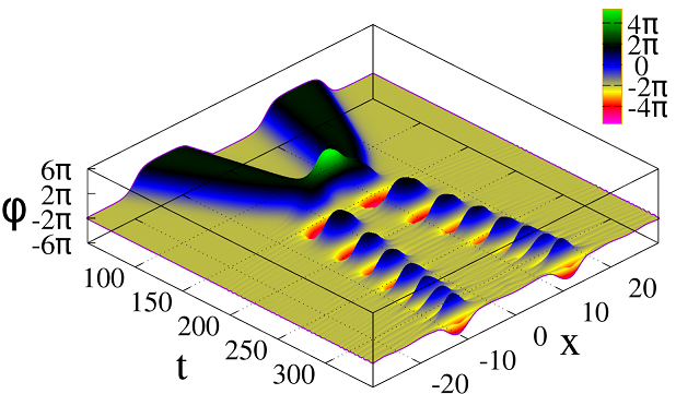
(a)  $R=0.50$

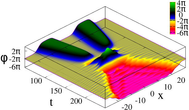
(b)  $R=1.0$

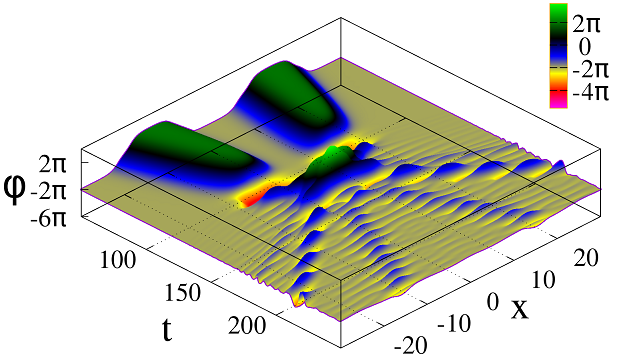
(c)  $R=1.5$

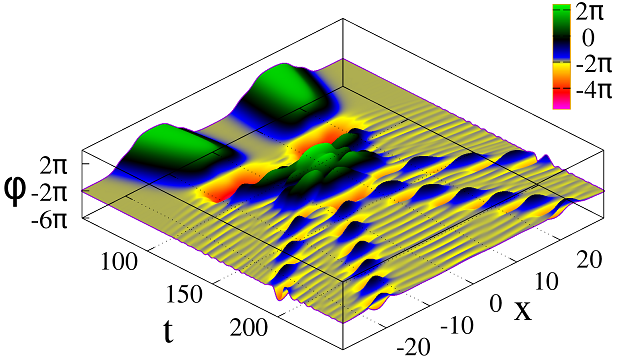
(d)  $R=2.0$

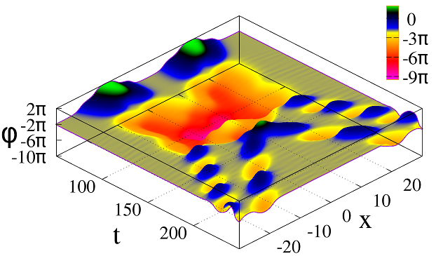
(e)  $R=2.5$

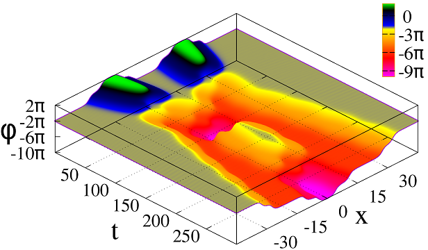
(f)  $R=3.0$

Figure 12: Space-time picture of collisions of four kinks for different $R$’s.

We can see a vast variety of final states. At $R=1.5$, $R=2.0$ and $R=2.5$ we observe four oscillons in the final state. We could propose the following explanation of the formation of oscillons. Each DSG kink/antikink consists of two subkinks, see Eq. (6). In the kinks collision the constituent subkinks interact with each other in a complicated way, thus forming bound states — oscillons. This means that we consider an oscillon as a bound state of subkinks (at the same time, remind that a bion is a bound state of kink and antikink). At $R=0.5$ we observe formation of two bions. At $R=1.0$ the final state has the form of escaping kink and antikink together with two oscillons also escaping from the collision point. At $R=3.0$ in the final state we see a bion localized near the origin $x=0$ and escaping DSG kink and antikink. Maximal values of the energy densities in the case of four kinks collisions are highly dependent on the initial positions of the kinks. That is why we did not study the energy densities here but briefly summarized the observed final states.

IV Discussion and conclusion

We have studied collisions of several kinks of the double sine-Gordon model in one point (in a small spatial region). We have performed numerical simulations of

• collisions of a kink and an antikink,

• collisions of two kinks and an antikink in one point,

• collisions of two kinks and two antikinks in one point.

Collisions of two kinks (i.e. kink-antikink scattering) are thoroughly investigated in literature Gani.EPJC.2018.dsg ; Gani.PRE.1999 ; Campbell.PhysD.1986.dsg . In this paper we focused on energy distributions in the kink-antikink collisions at various values of the parameter $R$. We have obtained $R$-dependences of the maximal (over $x$ and $t$) kinetic, gradient, potential and total energy densities, Fig. 5(d). The maximal kinetic, gradient and total energy densities behave rather stochastic at $0.5\stackrel{{\scriptstyle\scriptstyle<}}{{\phantom{}{}_{\sim}}}R\stackrel{{\scriptstyle\scriptstyle<}}{{\phantom{}{}_{\sim}}}2.5$, while at $R\stackrel{{\scriptstyle\scriptstyle<}}{{\phantom{}{}_{\sim}}}0.5$ and $R\stackrel{{\scriptstyle\scriptstyle>}}{{\phantom{}{}_{\sim}}}2.5$ smooth and monotonous segments are observed. We suppose that such behavior could be a consequence of the fact that the initial velocity of the kinks $v_{\mathrm{in}}=0.1$ is less than the critical velocity $v_{\mathrm{cr}}$, see Gani.EPJC.2018.dsg . This, in turn, leads to kinks’ capture and formation of a bion. Energy redistribution in a bion is complicated and can be viewed as chaotic. At the same time, at $R\stackrel{{\scriptstyle\scriptstyle<}}{{\phantom{}{}_{\sim}}}0.5$ and $R\stackrel{{\scriptstyle\scriptstyle>}}{{\phantom{}{}_{\sim}}}2.5$ we have $v_{\mathrm{in}}>v_{\mathrm{cr}}$, and colliding kinks bounce off each other after the first impact. In this case the complex energy redistribution does not take place, and $R$-dependences of the maximal energy densities are smooth and monotonous.

Besides, at $1.5\stackrel{{\scriptstyle\scriptstyle<}}{{\phantom{}{}_{\sim}}}R\stackrel{{\scriptstyle\scriptstyle<}}{{\phantom{}{}_{\sim}}}1.6$ we also observed small smooth and monotonous segments of the maximal energy densities in Fig. 5(d). In this range of the parameter, unlike other close values of $R$, in the final state we have two escaping oscillons formed after two oscillations of the kink-antikink bound state.

In three kinks collisions (in collisions of two kinks and an antikink) we observed various final states, in particular, similar to (i) excited kink ($R=0.5$, Fig. 9(a)), (ii) excited kink and escaping oscillons ($R=1.0,1.5,2.0,2.5$, Figs. 9(b)–9(e)), and (iii) two escaping kinks and an antikink at rest ($R=3.0$, Fig. 9(f)). The maximal kinetic, gradient and total energy densities behave stochastic. At the same time, within the range $1.7\stackrel{{\scriptstyle\scriptstyle<}}{{\phantom{}{}_{\sim}}}R\stackrel{{\scriptstyle\scriptstyle<}}{{\phantom{}{}_{\sim}}}2.1$ we observed smooth and monotonous segments of the curves. We found that it could be a consequence of the formation of two escaping oscillons in the final state right after the kinks collision. Notice that the maximal total energy density in three-kink collisions is considerably larger than in two-kink collisions, see Figs. 5(d) and 10. At the same time, the maximal potential energy density is nearly the same for the two- and three-kink collisions. It means that the collision process does not affect on the maximal potential energy density. It is interesting that similar situation was observed in the multi-kink collisions in the sine-Gordon model Moradi.EPJB.2017.multikink (up to seven kinks collision) and in the collisions of odd number of kinks in the $\varphi^{4}$ (up to five kinks collision) Moradi.CNSNS.2017.multikink , while in the collisions of even number of kinks in the $\varphi^{4}$ (up to four kinks collision) and in the $\varphi^{6}$ multi-kink collisions the maximal potential energy depends on the number of colliding kinks Moradi.JHEP.2017.multikink ; Moradi.CNSNS.2017.multikink .

Finally, we have studied collisions of four kinks (two kinks and two antikinks). The initial positions and velocities of the kinks were fit in such a way in order to provide almost simultaneous collision of all four waves in one point. After collision we observed a vast variety of the final states. Besides, the maximal energy densities strongly depend on the initial positions of the colliding kinks. That is why the analysis of the maximal energy densities requires detailed investigation of their dependences on parameters of the initial condition, which could be a subject of a separate publication. In this paper we have limited ourselves to the classification of the most typical final configurations. In particular, at $R=0.5$ in the final state we observed two oscillating structures which we classified as bound states of the DSG kink and antikink. At $R=1.0$ we observed escaping kink and antikink along with two oscillons — bound states of subkinks, which are components of the DSG kink (antikink). At $R=1.5$ and $R=2.0$ — only oscillons, at $R=3.0$ — escaping antikink and kink, while the other kink-antikink pair forms a bion localized near the collision point.

So we see a vast variety of final states in collisions of more than two kinks. Moreover, the behavior of the maximal energy densities strongly depends on oscillating structures being formed in the final state.

In conclusion, we would like to mention the following issues which are beyond the scope of our paper, nevertheless, in our opinion, could become subject to future work.

• First, the multi-kink scattering within the field-theoretic models with polynomial potentials of 8th or higher degrees. As we have already mentioned in the Introduction, such models can have kinks with long-range interaction between them due to the kinks’ power-law tails. This long-range interaction could lead to new collective phenomena in multi-kink systems.

• Second, the multi-kink scattering within models with non-polynomial potentials, e.g., sinh-deformed $\varphi^{4}$ or $\varphi^{6}$, could be of interest, and will be studied in a separate publication.

References

- (1) R. Rajaraman, Solitons and Instantons: An Introduction to Solitons and Instantons in Quantum Field Theory (North-Holland, Amsterdam, 1982)
- (2) A. Vilenkin, E.P.S. Shellard, Cosmic Strings and Other Topological Defects (Cambridge University Press, Cambridge, 2000)
- (3) N. Manton, P. Sutcliffe, Topological Solitons (Cambridge University Press, Cambridge, 2004)
- (4) T. Vachaspati, Kinks and Domain Walls: An Introduction to Classical and Quantum Solitons (Cambridge University Press, Cambrifge, 2006)
- (5) V.A. Gani, A.E. Kudryavtsev, M.A. Lizunova, Kink interactions in the (1+1)-dimensional model. Phys. Rev. D 89, 125009 (2014). arXiv:1402.5903
- (6) V.A. Gani, V. Lensky, M.A. Lizunova, Kink excitation spectra in the (1+1)-dimensional model. JHEP 08, 147 (2015). arXiv:1506.02313
- (7) V.A. Gani, V. Lensky, M.A. Lizunova, E.V. Mrozovskaya, Excitation spectra of solitary waves in scalar field models with polynomial self-interaction. J. Phys.: Conf. Ser. 675, 012019 (2016). arXiv:1602.02636
- (8) D. Bazeia, E. Belendryasova, V.A. Gani, Scattering of kinks of the sinh-deformed model. Eur. Phys. J. C 78, 340 (2018). arXiv:1710.04993
- (9) D. Bazeia, E. Belendryasova, V.A. Gani, Scattering of kinks in a non-polynomial model. J. Phys.: Conf. Ser. 934, 012032 (2017). arXiv:1711.07788
- (10) V.A. Gani, A. Moradi Marjaneh, A. Askari, E. Belendryasova, D. Saadatmand, Scattering of the double sine-Gordon kinks. Eur. Phys. J. C 78, 345 (2018). arXiv:1711.01918
- (11) E. Belendryasova, V.A. Gani, A. Moradi Marjaneh, D. Saadatmand, A. Askari, A new look at the double sine-Gordon kink-antikink scattering. J. Phys.: Conf. Ser. 1205, 012007 (2019). arXiv:1810.00667
- (12) A.R. Gomes, F.C. Simas, K.Z. Nobrega, P.P. Avelino, False vacuum decay in kink scattering. JHEP 10, 192 (2018). arXiv:1805.00991
- (13) D. Bazeia, A.R. Gomes, K.Z. Nobrega, F.C. Simas, Kink scattering in a hybrid model. Phys. Lett. B 793, 26 (2019). arXiv:1805.07017
- (14) P. Dorey, T. Romańczukiewicz, Resonant kink-antikink scattering through quasinormal modes. Phys. Lett. B 779, 117 (2018). arXiv:1712.10235
- (15) J.G.F. Campos, A. Mohammadi, Quasinormal modes in kink-antikink interactions: a toy model. arXiv:1905.00835
- (16) Y. Zhong, Z.-C. Jiang, Y.-X. Liu, Y.-Q. Wang, Collision of two kinks with inner structure. arXiv:1906.02920
- (17) D.K. Campbell, M. Peyrard, Solitary wave collisions revisited. Physica D 18, 47 (1986)
- (18) T.I. Belova, A.E. Kudryavtsev, Solitons and their interactions in classical field theory. Phys. Usp. 40, 359 (1997)
- (19) T.I. Belova, A.E. Kudryavtsev, Solitons and their interactions in classical field theory. Usp. Fiz. Nauk 167, 377 (1997)
- (20) V.A. Gani, A.E. Kudryavtsev, Kink-antikink interactions in the double sine-Gordon equation and the problem of resonance frequencies. Phys. Rev. E 60, 3305 (1999). cond-mat/9809015
- (21) P. Dorey, K. Mersh, T. Romańczukiewicz, Y. Shnir, Kink-antikink collisions in the model. Phys. Rev. Lett. 107, 091602 (2011). arXiv:1101.5951
- (22) E. Belendryasova, V.A. Gani, Scattering of the kinks with power-law asymptotics. Commun. Nonlinear Sci. Numer. Simulat. 67, 414 (2019). arXiv:1708.00403
- (23) E. Belendryasova, V.A. Gani, Resonance phenomena in the kinks scattering. J. Phys.: Conf. Ser. 934, 012059 (2017). arXiv:1712.02846
- (24) A.R. Gomes, R. Menezes, J.C.R.E. Oliveira, Highly interactive kink solutions. Phys. Rev. D 86, 025008 (2012). arXiv:1208.4747
- (25) R.V. Radomskiy, E.V. Mrozovskaya, V.A. Gani, I.C. Christov, Topological defects with power-law tails. J. Phys.: Conf. Ser. 798, 012087 (2017). arXiv:1611.05634
- (26) I.C. Christov, R.J. Decker, A. Demirkaya, V.A. Gani, P.G. Kevrekidis, R.V. Radomskiy, Long-range interactions of kinks. Phys. Rev. D 99, 016010 (2019). arXiv:1810.03590
- (27) I.C. Christov, R.J. Decker, A. Demirkaya, V.A. Gani, P.G. Kevrekidis, A. Khare, A. Saxena, Kink-kink and kink-antikink interactions with long-range tails. Phys. Rev. Lett. 122, 171601 (2019). arXiv:1811.07872
- (28) N.S. Manton, Force between kinks with long-range tails. arXiv:1810.00788
- (29) N.S. Manton, Forces between kinks and antikinks with long-range tails. J. Phys. A: Math. Theor. 52, 065401 (2019). arXiv:1810.03557
- (30) D. Bazeia, R. Menezes, D.C. Moreira, Analytical study of kinklike structures with polynomial tails. J. Phys. Commun. 2, 055019 (2018). arXiv:1805.09369
- (31) I. Takyi, H. Weigel, Collective coordinates in one-dimensional soliton models revisited. Phys. Rev. D 94, 085008 (2016). arXiv:1609.06833
- (32) A. Demirkaya, R. Decker, P.G. Kevrekidis, I.C. Christov, A. Saxena, Kink dynamics in a parametric system: a model with controllably many internal modes. JHEP 12, 071 (2017). arXiv:1706.01193
- (33) J.K. Perring, T.H.R. Skyrme, A model unified field equation. Nucl. Phys. 31, 550 (1962)
- (34) R. Rajaraman, Intersoliton forces in weak-coupling quantum field theories. Phys. Rev. D 15, 2866 (1977)
- (35) N.S. Manton, An effective Lagrangian for solitons. Nucl. Phys. B 150, 397 (1979)
- (36) P.G. Kevrekidis, A. Khare, A. Saxena, Solitary wave interactions in dispersive equations using Manton’s approach. Phys. Rev. E 70, 057603 (2004). nlin/0410045
- (37) V.A. Gani, A.E. Kudryavtsev, Collisions of domain walls in a supersymmetric model. Phys. Atom. Nucl. 64, 2043 (2001). hep-th/9904209
- (38) V.A. Gani, A.E. Kudryavtsev, Collisions of domain walls in a supersymmetric model. Yad. Fiz. 64, 2130 (2001). hep-th/9912211
- (39) V.A. Lensky, V.A. Gani, A.E. Kudryavtsev, Domain walls carrying a U(1) charge. Sov. Phys. JETP 93, 677 (2001). hep-th/0104266
- (40) V.A. Lensky, V.A. Gani, A.E. Kudryavtsev, Domain walls carrying a U(1) charge. Zh. Eksp. Teor. Fiz. 120, 778 (2001). hep-th/0104266
- (41) A. Alonso Izquierdo, M.A. Gonzalez Leon, J. Mateos Guilarte, The Kink variety in systems of two coupled scalar fields in two space-time dimensions. Phys. Rev. D 65, 085012 (2002). hep-th/0201200
- (42) V.A. Gani, N.B. Konyukhova, S.V. Kurochkin, V.A. Lensky, Study of stability of a charged topological soliton in the system of two interacting scalar fields. Comput. Math. Math. Phys. 44, 1968 (2004). arXiv:0710.2975
- (43) V.A. Gani, N.B. Konyukhova, S.V. Kurochkin, V.A. Lensky, Study of stability of a charged topological soliton in the system of two interacting scalar fields. Zh. Vychisl. Mat. Mat. Fiz. 44, 2069 (2004). arXiv:0710.2975
- (44) A. Alonso Izquierdo, D. Bazeia, L. Losano, J. Mateos Guilarte, New Models for Two Real Scalar Fields and Their Kink-Like Solutions. Adv. in High Energy Phys. 2013, 183295 (2013). arXiv:1308.2724
- (45) A. Alonso Izquierdo, J. Mateos Guilarte, Quantum-induced interactions in the moduli space of degenerate BPS domain walls. J. High Energy Phys. 01, 125 (2014). arXiv:1307.0740
- (46) H. Katsura, Composite-kink solutions of coupled nonlinear wave equations. Phys. Rev. D 89, 085019 (2014). arXiv:1312.4263
- (47) A. Alonso Izquierdo, Kink dynamics in a system of two coupled scalar fields in two space-time dimensions. Physica D 365, 12 (2018). arXiv:1711.08784
- (48) A. Alonso Izquierdo, Reflection, transmutation, annihilation, and resonance in two-component kink collisions. Phys. Rev. D 97, 045016 (2018). arXiv:1711.10034
- (49) A. Alonso Izquierdo, Kink dynamics in the MSTB Model. Phys. Scr. 94, 085302 (2019). arXiv:1804.05605
- (50) A. Alonso Izquierdo, Asymmetric kink scattering in a two-component scalar field theory model. Commun. Nonlinear Sci. Numer. Simulat. 75, 200 (2019). arXiv:1901.03089
- (51) J.R. Morris, Interacting kinks and meson mixing. Ann. Phys. 400, 346 (2019). arXiv:1901.01467
- (52) A. Alonso Izquierdo, Non-topological kink scattering in a two-component scalar field theory model. arXiv:1906.05040
- (53) M. Mohammadi, N. Riazi, The affective factors on the uncertainty in the collisions of the soliton solutions of the double field sine-Gordon system. Commun. Nonlinear Sci. Numer. Simulat. 72, 176 (2019). arXiv:1906.07498
- (54) V.A. Gani, M.A. Lizunova, R.V. Radomskiy, Scalar triplet on a domain wall: an exact solution. JHEP 04, 043 (2016). arXiv:1601.07954
- (55) V.A. Gani, M.A. Lizunova, R.V. Radomskiy, Scalar triplet on a domain wall. J. Phys.: Conf. Ser. 675, 012020 (2016). arXiv:1602.04446
- (56) N. Blyankinshtein, Q-lumps on a domain wall with a spin-orbit interaction. Phys. Rev. D 93, 065030 (2016). arXiv:1510.07935
- (57) V.A. Gani, V.G. Ksenzov, A.E. Kudryavtsev, Example of a self-consistent solution for a fermion on domain wall. Phys. Atom. Nucl. 73, 1889 (2010). arXiv:1001.3305
- (58) V.A. Gani, V.G. Ksenzov, A.E. Kudryavtsev, Example of a self-consistent solution for a fermion on domain wall. Yad. Fiz. 73, 1940 (2010). arXiv:1001.3305
- (59) V.A. Gani, V.G. Ksenzov, A.E. Kudryavtsev, Stable branches of a solution for a fermion on domain wall. Phys. Atom. Nucl. 74, 771 (2011). arXiv:1009.4370
- (60) V.A. Gani, V.G. Ksenzov, A.E. Kudryavtsev, Stable branches of a solution for a fermion on domain wall. Yad. Fiz. 74, 797 (2011). arXiv:1009.4370
- (61) Y. Brihaye, A. Cisterna, B. Hartmann, G. Luchini, From topological to nontopological solitons: Kinks, domain walls, and Q-balls in a scalar field model with a nontrivial vacuum manifold. Phys. Rev. D 92, 124061 (2015). arXiv:1511.02757
- (62) A.Yu. Loginov, Q kink of the nonlinear O(3) model involving an explicitly broken symmetry. Phys. Atom. Nucl. 74, 740 (2011)
- (63) A.Yu. Loginov, Q kink of the nonlinear O(3) model involving an explicitly broken symmetry. Yad. Fiz. 74, 766 (2011)
- (64) D. Bazeia, A. Mohammadi, Fermionic bound states in distinct kinklike backgrounds. Eur. Phys. J. C 77, 203 (2017). arXiv:1702.00891
- (65) D. Bazeia, A. Mohammadi, D. C. Moreira, Fermion bound states in geometrically deformed backgrounds. Chin. Phys. C 43, 013101 (2019). arXiv:1706.04406
- (66) M. Mai, P. Schweitzer, Energy momentum tensor, and the D-term of Q-balls. Phys. Rev. D 86, 076001 (2012). arXiv:1206.2632
- (67) M. Mai, P. Schweitzer, Radial excitations of Q-balls, and their D-term. Phys. Rev. D 86, 096002 (2012). arXiv:1206.2930
- (68) M. Cantara, M. Mai, P. Schweitzer, The energy-momentum tensor and D-term of Q-clouds. Nucl. Phys. A 953, 1 (2016). arXiv:1510.08015
- (69) I.E. Gulamov, E.Ya. Nugaev, M.N. Smolyakov, Analytic Q-ball solutions and their stability in a piecewise parabolic potential. Phys. Rev. D 87, 085043 (2013). arXiv:1303.1173
- (70) D. Bazeia, M.A. Marques, R. Menezes, Exact solutions, energy and charge of stable Q-balls. Eur. Phys. J. C 76, 241 (2016). arXiv:1512.04279
- (71) D. Bazeia et al., Compact Q-balls. Phys. Lett. B 758, 146 (2016). arXiv:1604.08871
- (72) D. Bazeia, L. Losano, M.A. Marques, R. Menezes, Split Q-balls. Phys. Lett. B 765, 359 (2017). arXiv:1612.04442
- (73) D. Levkov, E. Nugaev, A. Popescu, The fate of small classically stable Q-balls. JHEP 12, 131 (2017). arXiv:1711.05279
- (74) V. Loiko, I. Perapechka, Ya. Shnir, Q-balls without a potential. Phys. Rev. D 98, 045018 (2018). arXiv:1805.11929
- (75) A. Kovtun, E. Nugaev, A. Shkerin, Vibrational modes of Q-balls. Phys. Rev. D 98, 096016 (2018). arXiv:1805.03518
- (76) A.Yu. Loginov, A two-dimensional soliton system of vortex and Q-ball. Phys. Lett. B 777, 340 (2018). arXiv:1901.00993
- (77) A.Yu. Loginov, One-dimensional soliton system of gauged Q-ball and anti-Q-ball. Phys. Rev. D 99, 065011 (2019). arXiv:1901.00272
- (78) E. Greenwood, E. Halstead, R. Poltis, D. Stojkovic, Electroweak vacua, collider phenomenology, and possible connection with dark energy. Phys. Rev. D 79, 103003 (2009). arXiv:0810.5343
- (79) D. Castañeda Valle, E.W. Mielke, Relativistic soliton collisions of axion type dark matter. Phys. Lett. B 758, 93 (2016)
- (80) Y. Matsui, K. Horiguchi, D. Nitta, S. Kuroyanagi, Improved calculation of the gravitational wave spectrum from kinks on infinite cosmic strings. JCAP 11, 005 (2016). arXiv:1605.08768
- (81) J.M. Wachter, K.D. Olum, Gravitational Smoothing of Kinks on Cosmic String Loops. Phys. Rev. Lett. 118, 051301 (2017). arXiv:1609.01153
- (82) J. Ye, K. Wang, Y.F. Cai, Superconducting cosmic strings as sources of cosmological fast radio bursts. Eur. Phys. J. C 77, 720 (2017). arXiv:1705.10956
- (83) C. Ringeval, T. Suyama, Stochastic gravitational waves from cosmic string loops in scaling. JCAP 12, 027 (2017). arXiv:1709.03845
- (84) V.A. Gani, A.A. Kirillov, S.G. Rubin, Classical transitions with the topological number changing in the early Universe. JCAP 04, 042 (2018). arXiv:1704.03688
- (85) V.A. Gani, A.A. Kirillov, S.G. Rubin, Transitions between topologically non-trivial configurations. J. Phys.: Conf. Ser. 934, 012046 (2017). arXiv:1711.07700
- (86) D. Saadatmand, S.V. Dmitriev, P.G. Kevrekidis, High energy density in multisoliton collisions. Phys. Rev. D 92, 056005 (2015). arXiv:1506.01389
- (87) A. Moradi Marjaneh, V.A. Gani, D. Saadatmand, S.V. Dmitriev, K. Javidan, Multi-kink collisions in the model. JHEP 07, 028 (2017). arXiv:1704.08353
- (88) A. Moradi Marjaneh, A. Askari, D. Saadatmand, S.V. Dmitriev, Extreme values of elastic strain and energy in sine-Gordon multi-kink collisions. Eur. Phys. J. B 91, 22 (2017). arXiv:1710.10159
- (89) A. Moradi Marjaneh, D. Saadatmand, K. Zhou, S.V. Dmitriev, M.E. Zomorrodian, High energy density in the collision of kinks in the model. Commun. Nonlinear Sci. Numer. Simulat. 49, 30 (2017). arXiv:1605.09767
- (90) A. Askari, D. Saadatmand, S.V. Dmitriev, K. Javidan, High energy density spots and production of kink-antikink pairs in particle collisions. Wave Motion 78, 54 (2018). arXiv:1608.01847
- (91) D.K. Campbell, M. Peyrard, P. Sodano, Kink-antikink interactions in the double sine-Gordon equation. Physica D 19, 165 (1986)
- (92) B.A. Malomed, Dynamics and kinetics of solitons in the driven damped double sine-Gordon equation. Phys. Lett. A 136, 395 (1989)
- (93) S. Nazifkar, K. Javidan, Collective coordinate analysis for double sine-Gordon model. Braz. J. Phys. 40, 102 (2010)