Abstract

BACKGROUND
Indicators of relative inequality of lifespans are important because they capture the dimensionless shape of aging. They are markers of inequality at the population level and express the uncertainty at the time of death at the individual level. In particular, Keyfitz’ entropy  $H$ represents the elasticity of life expectancy to a change in mortality and it has been used as an indicator of lifespan variation. However, it is unknown how this measure changes over time and whether a threshold age exists, as it does for other lifespan variation indicators.

RESULTS
The time derivative of  $H$ can be decomposed into changes in life disparity $e^{\dagger}$ and life expectancy at birth $e_{o}$. Likewise, changes over time in  $H$ are a weighted average of age-specific rates of mortality improvements. These weights reflect the sensitivity of  $H$ and show how mortality improvements can increase (or decrease) the relative inequality of lifespans. Further, we prove that  $H$ , as well as $e^{\dagger}$, in the case that mortality is reduced in every age, has a threshold age below which saving lives reduces entropy, whereas improvements above that age increase entropy.

CONTRIBUTION
We give a formal expression for changes over time of  $H$ and provide a formal proof of the threshold age that separates reductions and increases in lifespan inequality from age-specific mortality improvements.

1 Relationship

Keyfitz’ entropy is a dimensionless indicator of the relative variation in the length of life compared to life expectancy (Keyfitz 1977; Demetrius 1978). It is usually defined as

$$\hbox{\vbox{\hrule height=0.5pt\kern 1.29167pt\hbox{\kern-2.5pt$H$\kern-0.50003pt}}}(t)=-\frac{\int_{0}^{\infty}\ell(a,t)\,\ln\ell(a,t)\,da}{\int_{0}^{\infty}\ell(a,t)\,da}=\int_{0}^{\infty}c(a,t)\,H(a,t)\,da=\frac{e^{\dagger}(t)}{e_{o}(t)}\;,$$

where $e^{\dagger}(t)=-\int_{0}^{\infty}\ell(a,t)\,\ln\ell(a,t)\,da$ is the life disparity or number of life-years lost as a result of death (Vaupel and Canudas-Romo 2003), $e_{o}(t)=\int_{0}^{\infty}\ell(a,t)\,da$ is the life expectancy at birth at time $t$, $\ell(a,t)$ is the life table survival function, $c(a,t)=\ell(a)\,/\,\int_{0}^{\infty}\ell(x)\,dx$ is the population structure, and $H(a,t)=\int_{0}^{a}\mu(x,t)\,dx$ is the cumulative hazard to age $a$, where $\mu(x,t)$ is the force of mortality (hazard rate or risk of death) at age $x$ at time $t$. Note that $\hbox{\vbox{\hrule height=0.5pt\kern 1.29167pt\hbox{\kern-2.5pt$H$\kern-0.50003pt}}}(t)$ can be interpreted as an average value of $H(a,t)$ in the population at time $t$.

Goldman and Lord (1986) and Vaupel (1986) proved that

$$e^{\dagger}(t)=\int_{0}^{\infty}d(a,t)\,e(a,t)\,da\;,$$

where $d(a,t)$ represents the distribution of deaths and $e(a,t)=\int_{a}^{\infty}\ell(x,t)\,dx\,/\,\ell(a,t)$ the remaining life expectancy at age $a$. This provides an alternative expression for Keyfitz’ entropy:

$$\hbox{\vbox{\hrule height=0.5pt\kern 1.29167pt\hbox{\kern-2.5pt$H$\kern-0.50003pt}}}(t)=\frac{\int_{0}^{\infty}d(a,t)\,e(a,t)\,da}{\int_{0}^{\infty}\ell(a,t)\,da}\;.$$

Let $\dot{\hbox{\vbox{\hrule height=0.5pt\kern 1.29167pt\hbox{\kern-2.5pt$H$\kern-0.50003pt}}}}$ denote the partial derivative of  $H$ with respect to time. We define $\rho(x)=-\dot{\mu}(x)\,/\,\mu(x)$ as the age-specific rates of mortality improvements. Then, the relative derivative of  $H$ can be expressed as a weighted average of age-specific rates of mortality improvement,

(1) $$\dot{\hbox{\vbox{\hrule height=0.5pt\kern 1.29167pt\hbox{\kern-2.5pt$H$\kern-0.50003pt}}}}\,/\,\hbox{\vbox{\hrule height=0.5pt\kern 1.29167pt\hbox{\kern-2.5pt$H$\kern-0.50003pt}}}=\int_{0}^{\infty}\rho(x)\,w(x)\,W(x)\,dx\;,$$

with weights

$$w(x)=\mu(x)\,\ell(x)\,e(x)\qquad\text{and}\qquad W(x)=\frac{1}{e^{\dagger}}\,\big{(}H(x)+\hbox{\vbox{\hrule height=0.5pt\kern 1.29167pt\hbox{\kern-2.5pt$H$\kern-0.50003pt}}}(x)-1\big{)}-\frac{1}{e_{o}}\;.$$

Function $\hbox{\vbox{\hrule height=0.5pt\kern 1.29167pt\hbox{\kern-2.5pt$H$\kern-0.50003pt}}}(x)$ is Keyfitz’ entropy conditioned on surviving to age $x$, defined as

$$\hbox{\vbox{\hrule height=0.5pt\kern 1.29167pt\hbox{\kern-2.5pt$H$\kern-0.50003pt}}}(x)=\frac{e^{\dagger}(x)}{e(x)}=\frac{\int_{x}^{\infty}d(a)\,e(a)\,da}{\int_{x}^{\infty}\ell(a)\,da}\,.$$

where $e^{\dagger}(x)=\int_{x}^{\infty}d(a)\,e(a)\,da\,/\,\ell(x)$ refers to life disparity above age $x$, and $e(x)$ is the remaining life expectancy at age $x$.

Note that Keyfitz’ entropy  $H$ is a measure of lifespan inequality. Thus, higher values represent more lifespan disparity, whereas lower values denote less variation of lifespans. If mortality improvements over time occur at all ages, there exists a unique threshold age $a^{H}$ that separates positive from negative contributions to Keyfitz’ entropy  $H$ resulting from those mortality improvements. This threshold age $a^{H}$ is reached when

(2) $$H\left(a^{H}\right)+\hbox{\vbox{\hrule height=0.5pt\kern 1.29167pt\hbox{\kern-2.5pt$H$\kern-0.50003pt}}}\left(a^{H}\right)=1+\hbox{\vbox{\hrule height=0.5pt\kern 1.29167pt\hbox{\kern-2.5pt$H$\kern-0.50003pt}}}\;.$$

2 Proof

Fernández and Beltrán-Sánchez (2015) showed that the relative derivative of  $H$ can be expressed as

(3) $$\dot{\hbox{\vbox{\hrule height=0.5pt\kern 1.29167pt\hbox{\kern-2.5pt$H$\kern-0.50003pt}}}}\,/\,\hbox{\vbox{\hrule height=0.5pt\kern 1.29167pt\hbox{\kern-2.5pt$H$\kern-0.50003pt}}}=\frac{\dot{e}^{\dagger}}{e^{\dagger}}-\frac{\dot{e}_{o}}{e_{o}}\;,$$

This formula indicates that relative changes in  $H$ over time are given by the difference between relative changes in $e^{\dagger}$ (dispersion component) and relative changes in $e_{o}$ (translation component). We will first provide expressions for $\dot{e}_{o}$ and $\dot{e}^{\dagger}$ to prove that (1) and (3) are equivalent. Next, we will prove the existence of threshold age for  $H$ and its uniqueness.

2.1 Relative changes over time in  $H$

Vaupel and Canudas-Romo (2003) showed that changes over time in life expectancy at birth are a weighted average of the total rates of mortality improvements:

(4) $$\dot{e}_{o}=\int_{0}^{\infty}\rho(x)\,w(x)\,dx\;,$$

where $\rho(x)=-\dot{\mu}(x)\,/\,\mu(x)$ are the age-specific rates of mortality improvement, and $w(x)=\mu(x)\,\ell(x)\,e(x)=d(x)e(x)$ is a measure of the importance of death at age $x$.

Since $d(x)=\mu(x)\,\ell(x)$ and $\ell(x)\,e(x)=\int_{x}^{\infty}\ell(a)\,da$, the partial derivative with respect to time of $e^{\dagger}=\int_{0}^{\infty}d(a)\,e(a)\,da$ can be expressed as

$$\begin{split}\dot{e}^{\dagger}&=\int_{0}^{\infty}\dot{\mu}(x)\,\ell(x)\,e(x)\,dx+\int_{0}^{\infty}\mu(x)\int_{x}^{\infty}\dot{\ell}(a)\,da\,dx\\ &=-\int_{0}^{\infty}\rho(x)\,w(x)\,dx+\int_{0}^{\infty}\dot{\ell}(a)\int_{0}^{a}\mu(x)\,dx\,da\\ &=-\int_{0}^{\infty}\rho(x)\,w(x)\,dx+\int_{0}^{\infty}\dot{\ell}(a)\,H(a)\,da\\ &=-\int_{0}^{\infty}\rho(x)\,w(x)\,dx-\int_{0}^{\infty}\int_{0}^{a}\dot{\mu}(x)\,dx\,\ell(a)\,H(a)\,da\;,\end{split}$$

where $H(a)$ is the cumulative hazard to age $a$. By reversing the order of integration and doing some additional manipulations, we get

(5) $$\begin{split}\dot{e}^{\dagger}&=-\int_{0}^{\infty}\rho(x)\,w(x)\,dx-\int_{0}^{\infty}\dot{\mu}(x)\int_{x}^{\infty}\,\ell(a)\,H(a)\,da\,dx\\ &=-\int_{0}^{\infty}\rho(x)\,w(x)\,dx+\int_{0}^{\infty}\rho(x)\,w(x)\,\frac{\int_{x}^{\infty}\,\ell(a)\,H(a)\,da}{\ell(x)\,e(x)}\,dx\\ &=\int_{0}^{\infty}\rho(x)\,w(x)\left(\frac{\int_{x}^{\infty}\,\ell(a)\big{(}H(a)-H(x)+H(x)\big{)}\,da}{\ell(x)\,e(x)}-1\right)dx\\ &=\int_{0}^{\infty}\rho(x)\,w(x)\left(H(x)\,\frac{\int_{x}^{\infty}\,\ell(a)\,da}{\ell(x)\,e(x)}+\frac{\int_{x}^{\infty}\,\ell(a)\big{(}H(a)-H(x)\big{)}\,da}{\ell(x)\,e(x)}-1\right)\,dx\\ &=\int_{0}^{\infty}\rho(x)\,w(x)\left(H(x)+\frac{\int_{x}^{\infty}\,\ell(a)\big{(}H(a)-H(x)\big{)}\,da}{\ell(x)\,e(x)}-1\right)\,dx\;.\end{split}$$

In Proposition 1 in the Appendix, we prove that

(6) $$e^{\dagger}(x)=\frac{1}{\ell(x)}\int_{x}^{\infty}d(a)\,e(a)\,da=\frac{1}{\ell(x)}\int_{x}^{\infty}\,\ell(a)\big{(}H(a)-H(x)\big{)}\,da\;.$$

Replacing (6) into (5) yields

(7) $$\begin{split}\dot{e}^{\dagger}&=\int_{0}^{\infty}\rho(x)\,w(x)\left(H(x)+\frac{e^{\dagger}(x)}{e(x)}-1\right)dx\\ &=\int_{0}^{\infty}\rho(x)\,w(x)\big{(}H(x)+\hbox{\vbox{\hrule height=0.5pt\kern 1.29167pt\hbox{\kern-2.5pt$H$\kern-0.50003pt}}}(x)-1\big{)}\,dx\;.\end{split}$$

Finally, replacing the expressions of $\dot{e}_{o}$ and $\dot{e}^{\dagger}$ from (4) and (7) into (3), we get

$$\begin{split}\dot{\hbox{\vbox{\hrule height=0.5pt\kern 1.29167pt\hbox{\kern-2.5pt$H$\kern-0.50003pt}}}}\,/\,\hbox{\vbox{\hrule height=0.5pt\kern 1.29167pt\hbox{\kern-2.5pt$H$\kern-0.50003pt}}}&=\frac{1}{e^{\dagger}}\int_{0}^{\infty}\rho(x)\,w(x)\left(H(x)+\hbox{\vbox{\hrule height=0.5pt\kern 1.29167pt\hbox{\kern-2.5pt$H$\kern-0.50003pt}}}(x)-1\right)dx-\frac{1}{e_{o}}\int_{0}^{\infty}\rho(x)\,w(x)\,dx\\ &=\int_{0}^{\infty}\rho(x)\,w(x)\left(\frac{1}{e^{\dagger}}\left(H(x)+\hbox{\vbox{\hrule height=0.5pt\kern 1.29167pt\hbox{\kern-2.5pt$H$\kern-0.50003pt}}}(x)-1\right)-\frac{1}{e_{o}}\right)dx\\ &=\int_{0}^{\infty}\rho(x)\,w(x)\,W(x)\,dx\;,\end{split}$$

which proves (1) and shows that relative changes over time in Keyfitz’ entropy are the average of the rates of mortality improvement weighted by the product $w(x)\,W(x)$. $\square$

2.2 The threshold age for  $H$

Using (1), changes over time in Keyfitz’ entropy  $H$ are given by the function

(8) $$\dot{\hbox{\vbox{\hrule height=0.5pt\kern 1.29167pt\hbox{\kern-2.5pt$H$\kern-0.50003pt}}}}=\hbox{\vbox{\hrule height=0.5pt\kern 1.29167pt\hbox{\kern-2.5pt$H$\kern-0.50003pt}}}\,\int_{0}^{\infty}\rho(x)\,w(x)\,W(x)\,dx\;.$$

If $\dot{\hbox{\vbox{\hrule height=0.5pt\kern 1.29167pt\hbox{\kern-2.5pt$H$\kern-0.50003pt}}}}>0$, lifespan inequality increases over time, whereas $\dot{\hbox{\vbox{\hrule height=0.5pt\kern 1.29167pt\hbox{\kern-2.5pt$H$\kern-0.50003pt}}}}<0$ implies that variation of lifespans decrease over time. Because $\ell(x)$ is a positive function bounded between 0 and 1, Keyfitz’ entropy $\hbox{\vbox{\hrule height=0.5pt\kern 1.29167pt\hbox{\kern-2.5pt$H$\kern-0.50003pt}}}>0$. Moreover, assuming age-specific death rates $\mu(x)$ improve over time for all ages, then $\dot{\mu}(x)<0$ and $\rho(x)>0$ at any age $x$. Therefore, (8) implies that

1. Those ages $x$ in which $w(x)\,W(x)>0$ will contribute positively to Keyfitz’ entropy  $H$ and increase lifespan variation;

2. Those ages $x$ in which $w(x)\,W(x)<0$ will contribute negatively to Keyfitz’ entropy  $H$ and favor lifespan equality;

3. Those ages $x$ in which $w(x)\,W(x)=0$ will have no effect on the variation over time of  $H$ .

Our goal is to prove that if mortality improvements occur for all ages and $\rho(x)>0$, there exists a unique threshold age $a^{H}$ such that $w\left(a^{H}\right)\,W\left(a^{H}\right)=0$. That threshold age will separate positive from negative contributions to  $H$ resulting from mortality improvements.

The product $w(x)\,W(x)$ can be re-expressed as

$$\begin{split}w(x)\,W(x)&=\mu(x)\,\ell(x)\,e(x)\,\left(\,\frac{1}{e^{\dagger}}\left(H(x)+\hbox{\vbox{\hrule height=0.5pt\kern 1.29167pt\hbox{\kern-2.5pt$H$\kern-0.50003pt}}}(x)-1\right)-\frac{1}{e_{o}}\right)\\ &=\frac{\mu(x)\,\ell(x)\,e(x)}{e^{\dagger}}\left(H(x)+\hbox{\vbox{\hrule height=0.5pt\kern 1.29167pt\hbox{\kern-2.5pt$H$\kern-0.50003pt}}}(x)-\hbox{\vbox{\hrule height=0.5pt\kern 1.29167pt\hbox{\kern-2.5pt$H$\kern-0.50003pt}}}-1\right)\;.\end{split}$$

Since $\mu(x)$, $\ell(x)$, $e(x)$ and $e^{\dagger}$ are all positive functions, the threshold age of  $H$ occurs when

(9) $$g(x)=H(x)+\hbox{\vbox{\hrule height=0.5pt\kern 1.29167pt\hbox{\kern-2.5pt$H$\kern-0.50003pt}}}(x)-\hbox{\vbox{\hrule height=0.5pt\kern 1.29167pt\hbox{\kern-2.5pt$H$\kern-0.50003pt}}}-1=0\;.$$

When $x$ is close to 0, $g(x)$ takes negative values since

$$g(0)=H(0)+\hbox{\vbox{\hrule height=0.5pt\kern 1.29167pt\hbox{\kern-2.5pt$H$\kern-0.50003pt}}}^{+}(0)-\hbox{\vbox{\hrule height=0.5pt\kern 1.29167pt\hbox{\kern-2.5pt$H$\kern-0.50003pt}}}-1=0+\hbox{\vbox{\hrule height=0.5pt\kern 1.29167pt\hbox{\kern-2.5pt$H$\kern-0.50003pt}}}-\hbox{\vbox{\hrule height=0.5pt\kern 1.29167pt\hbox{\kern-2.5pt$H$\kern-0.50003pt}}}-1=-1<0\;.$$

Likewise, $g(x)$ takes positive values when $x$ becomes arbitrary large. Note that  $H$ does not depend on age, and therefore

$$\lim_{x\to\infty}g(x)=\lim_{x\to\infty}\left(H(x)+\hbox{\vbox{\hrule height=0.5pt\kern 1.29167pt\hbox{\kern-2.5pt$H$\kern-0.50003pt}}}(x)\right)=\infty\;,$$

because $\lim_{x\to\infty}H(x)=\infty$. By definition, $\hbox{\vbox{\hrule height=0.5pt\kern 1.29167pt\hbox{\kern-2.5pt$H$\kern-0.50003pt}}}(x)\geq 0$ for all $x$, so regardless of the behavior of $\hbox{\vbox{\hrule height=0.5pt\kern 1.29167pt\hbox{\kern-2.5pt$H$\kern-0.50003pt}}}(x)$ when $x$ is arbitrarily large, the limit of $g(x)$ tends to infinity. Hence, given that $g(0)=-1$ and $\lim_{x\to\infty}g(x)=\infty$, in a continuous framework the intermediate value theorem guarantees the existence of at least one age $a^{H}$ at which $g(a^{H})=0$.

Moreover, as shown in Propostion 2 in the Appendix, $g(x)$ is an increasing function. Therefore, there is a unique threshold age $a^{H}$ that separates positive from negative contributions to Keyfitz’ entropy  $H$ , and that threshold age is reached when

$$w(x)\,W(x)=0\Longleftrightarrow g(x)=0\Longleftrightarrow H(x)+\hbox{\vbox{\hrule height=0.5pt\kern 1.29167pt\hbox{\kern-2.5pt$H$\kern-0.50003pt}}}(x)=1+\hbox{\vbox{\hrule height=0.5pt\kern 1.29167pt\hbox{\kern-2.5pt$H$\kern-0.50003pt}}}\;,$$

which proves (2). $\square$

3 Related results

Demographers have developed a battery of indicators to measure how lifespans vary in populations (Colchero et al. 2016; van Raalte and Caswell 2013). The most used indexes are the variance (Edwards and Tuljapurkar 2005; Tuljapurkar and Edwards 2011), standard deviation (van Raalte, Sasson, and Martikainen 2018), or coefficient of variation (Aburto et al. 2018) of the age at death distribution , the Gini coefficient (Shkolnikov, Andreev, and Begun 2003; Archer et al. 2018; Gigliarano, Basellini, and Bonetti 2017), Theil index (Smits and Monden 2009) and years of life lost (Vaupel, Zhang, and van Raalte 2011; Aburto and van Raalte 2018) among others. However, only few studies have analytically derived formulas for threshold age below and above which mortality improvements respectively decrease and increase lifespan variation. Zhang and Vaupel (2009) showed that the threshold age $(a^{\dagger})$ for life disparity $(e^{\dagger})$ occurs when $H(x)+\bar{H}(x)=1$. Similarly, Gillespie, Trotter, and Tuljapurkar (2014) determined a threshold age for the variance of the age at death distribution. van Raalte and Caswell (2013) also showed that it is possible to determine the threshold age by performing an empirical sensitivity analysis of lifespan variation indicators.

In this article, we contribute to the lifespan variation literature by deriving the threshold age $a^{H}$ for Keyfitz’ entropy. This age separates negative from positive contributions of age-specific mortality improvements. We analytically proved its existence and demonstrated in Section 4 that it differs from the threshold age of $e^{\dagger}$.

4 Applications

4.1 Numerical findings

Figure 1 depicts the threshold ages for the two related measures: $e^{\dagger}$ and  $H$ . Calculations were performed using data from the Human Mortality Database (2018) for females in the United States and Italy in 2005. The blue line represents $g(x)$ from Equation (9). The threshold age $a^{H}$ occurs when $g(x)$ crosses zero. The red and grey line display the same functions that Zhang and Vaupel (2009) used to find the threshold age for $e^{\dagger}$. The intersection of these two lines denotes the threshold age $a^{\dagger}$. Finally, the dashed black line depicts the life expectancy at birth. Vaupel, Zhang, and van Raalte (2011) noted that $a^{\dagger}$ tends to fall just below life expectancy. The threshold age for Keyfitz’ entropy $a^{H}$ is greater than $a^{\dagger}$ and is very close above life expectancy for these countries. Not the similarity of the formulas for $a^{\dagger}$ given by $H(a^{\dagger})+\bar{H}(a^{\dagger})=1$ and $a^{H}$ given by $H(a^{H})+\hbox{\vbox{\hrule height=0.5pt\kern 1.29167pt\hbox{\kern-2.5pt$H$\kern-0.50003pt}}}(a^{H})=1+\hbox{\vbox{\hrule height=0.5pt\kern 1.29167pt\hbox{\kern-2.5pt$H$\kern-0.50003pt}}}$.

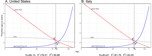
Figure 1: Derivation of threshold ages for $e^{\dagger}$ ($a^{\dagger}$) and Keyfitz’ entropy ($a^{H}$) from life table functions for United States and Italy in 2005. Source: Human Mortality Database (2018)

Panel A and B of Figure 2 illustrate the evolution of the threshold ages for $e^{\dagger}$ and  $H$ for females in France and Sweden respectively. We chose these countries because they portray large series of reliable data available through the Human Mortality Database (2018).

Values for $a^{\dagger}$ are close to life expectancy throughout the period. However, after around 1950 there is a crossover between $a^{\dagger}$ and $e_{o}$ such that $a^{\dagger}$ remained close to life expectancy but below it. This result shows that the threshold age $a^{\dagger}$ being below life expectancy is a modern feature of ageing populations with high life expectancy. From the beginning of the period of observation to the 1950s, the threshold age for Keyfitz’ entropy was above life expectancy for both countries. During some periods $a^{\dagger}$ was roughly constant whereas life expectancy trended upwards. After the 1950s, $a^{\dagger}$ converged towards life expectancy. The code and data to reproduce these results are publicly available through this repository [link not given to avoid identification of authors].

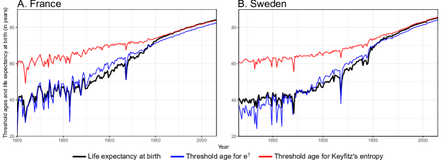
Figure 2: Threshold age for $e^{\dagger}$ and Keyftiz’ entropy  $H$ for females in France and Sweden over time. Source: Human Mortality Database (2018)

4.2 Decomposition of the relative derivative of  $H$

The relative derivative of  $H$ defined in Equation (1) can be decomposed between components before and after the threshold age $a^{H}$ as follows:

(10) $$\begin{split}\dot{\hbox{\vbox{\hrule height=0.5pt\kern 1.29167pt\hbox{\kern-2.5pt$H$\kern-0.50003pt}}}}\,/\,\hbox{\vbox{\hrule height=0.5pt\kern 1.29167pt\hbox{\kern-2.5pt$H$\kern-0.50003pt}}}&=\int_{0}^{\infty}\rho(x)\,w(x)\,W(x)\,dx\;\\ &=\int_{0}^{a^{H}}\rho(x)\,w(x)\,W(x)\,dx+\int_{a^{H}}^{\infty}\rho(x)\,w(x)\,W(x)\,dx\\ &=\underbrace{\left\{\frac{\dot{e}^{\dagger}[x|x<a^{H}]}{e^{\dagger}}-\frac{\dot{e}_{o}[x|x<a^{H}]}{e_{o}}\right\}}_{\textit{Early life component}}+\underbrace{\left\{\frac{\dot{e}^{\dagger}[x|x>a^{H}]}{e^{\dagger}}-\frac{\dot{e}_{o}[x|x>a^{H}]}{e_{o}}\right\}}_{\textit{Late life component}}\end{split}$$

If mortality reductions occur at every age, the early life component in Equation (10) is always positive (contributing to reduce entropy) while the late life component is negative (contributing to increasing entropy). Thus, it is clear that a negative relationship between life expectancy and entropy over time occurs if the early life component outpaces the late life component. This decomposition is based on the additive properties of the derivatives of life expectancy and $e^{\dagger}$ as previously shown in Vaupel and Canudas-Romo (2003) and Fernández and Beltrán-Sánchez (2015).

5 Conclusion

Several authors have been interested in decomposing changes over time in life expectancy (Arriaga 1984; Vaupel 1986; Pollard 1988; Vaupel and Canudas-Romo 2003; Beltrán-Sánchez, Preston, and Canudas-Romo 2008; Beltrán-Sánchez and Soneji 2011). Recently, authors have also investigated how life disparity fluctuations over time can be decomposed (Wagner 2010; Zhang and Vaupel 2009; Shkolnikov et al. 2011; Aburto and van Raalte 2018). In this paper, we bring both perspectives together and shed light on the dynamics behind changes in Keyfitz’ entropy.

Keyfitz (1977) first proposed  $H$ as a life table function that measures the change in life expectancy at birth consequent on a proportional change in age-specific rates. Since then, several authors have been interested in this measure and its use (Demetrius 1978, 1979; Mitra 1978; Goldman and Lord 1986; Vaupel 1986; Hakkert 1987; Hill 1993; Fernández and Beltrán-Sánchez 2015). Keyfitz’ entropy has become an appropriate indicator of lifespan variation that permits comparison of the shape of ageing across different species and over time (Baudisch et al. 2013; Wrycza, Missov, and Baudisch 2015). In this article, we uncover the mathematical regularities behind the changes over time in Keyfitz’ entropy. In particular, this study contributes to the existing literature by showing that (1) Keyfitz’ entropy can be decomposed as a weighted average of rates of mortality improvements and (2) that there exists a threshold age that separates positive and negative contributions of reductions in mortality over time.

Appendix

Proposition 1.

Let $e^{\dagger}(x)=\int_{x}^{\infty}d(a)\,e(a)\,da\,/\,\ell(x)$ be a measure of lifespan disparity above age $x$, where $d(a)$ accounts for the distribution of deaths, $e(a)$ the remaining life expectancy at age $a$, and $\ell(x)$ is the probability of surviving from birth to age $x$. Then,

(A1) $$e^{\dagger}(x)=\frac{1}{\ell(x)}\int_{x}^{\infty}\,\ell(a)\big{(}H(a)-H(x)\big{)}\,da\;,$$

where $H(x)$ is the cumulative hazard to age $x$.

Proof.

Note that

$$\frac{1}{\ell(x)}\int_{x}^{\infty}\,\ell(a)\big{(}H(a)-H(x)\big{)}\,da=\frac{1}{\ell(x)}\int_{x}^{\infty}\,\ell(a)\int_{x}^{a}\mu(y)\,dy\,da\;,$$

where function $\mu(y)$ is the force of mortality or hazard rate. By reversing the order of integration, and using that $e(y)=\int_{y}^{\infty}\ell(a)\,da\,/\,\ell(y)$ and $d(y)=\mu(y)\,\ell(y)$, we get

$$\begin{split}\frac{1}{\ell(x)}\int_{x}^{\infty}\,\ell(a)\int_{x}^{a}\mu(y)\,dy\,da&=\frac{1}{\ell(x)}\int_{x}^{\infty}\mu(y)\int_{y}^{\infty}\ell(a)\,da\,dy\\ &=\frac{1}{\ell(x)}\int_{x}^{\infty}\mu(y)\,\ell(y)\,e(y)\,dy\\ &=\frac{1}{\ell(x)}\int_{x}^{\infty}d(y)\,e(y)\,dy\\ &=e^{\dagger}(x)\;,\end{split}$$

which proves (A1). ∎

Proposition 2.

Let $\ell(x)$ be the probability of surviving from birth to age $x$. Let  $H$ be Keyfitz’ entropy and $\hbox{\vbox{\hrule height=0.5pt\kern 1.29167pt\hbox{\kern-2.5pt$H$\kern-0.50003pt}}}(x)=e^{\dagger}(x)\,/\,e(x)$ Keyfitz’ entropy conditioned on reaching age $x$. Let $H(x)$ be the cumulative hazard to age $x$. Then, $g(x)=H(x)+\hbox{\vbox{\hrule height=0.5pt\kern 1.29167pt\hbox{\kern-2.5pt$H$\kern-0.50003pt}}}(x)-1-\hbox{\vbox{\hrule height=0.5pt\kern 1.29167pt\hbox{\kern-2.5pt$H$\kern-0.50003pt}}}$ is an increasing function.

Proof.

In order to demonstrate that $g(x)$ is an increasing function it is sufficient to show that its first derivative is always positive. Hence, we must prove that

(A2) $$\frac{\partial}{\partial x}\,g(x)=\frac{\partial}{\partial x}\left(H(x)+\hbox{\vbox{\hrule height=0.5pt\kern 1.29167pt\hbox{\kern-2.5pt$H$\kern-0.50003pt}}}(x)-1-\hbox{\vbox{\hrule height=0.5pt\kern 1.29167pt\hbox{\kern-2.5pt$H$\kern-0.50003pt}}}\right)=\frac{\partial}{\partial x}\,H(x)+\frac{\partial}{\partial x}\hbox{\vbox{\hrule height=0.5pt\kern 1.29167pt\hbox{\kern-2.5pt$H$\kern-0.50003pt}}}(x)\geq 0$$

for all ages $x$.

By the fundamental theorem of calculus,

(A3) $$\frac{\partial}{\partial x}\,H(x)=\frac{\partial}{\partial x}\int_{0}^{x}\mu(a)\,da=\mu(x)\;,$$

whereas

$$\frac{\partial}{\partial x}\,\hbox{\vbox{\hrule height=0.5pt\kern 1.29167pt\hbox{\kern-2.5pt$H$\kern-0.50003pt}}}(x)=\frac{\partial}{\partial x}\,\left(\frac{e^{\dagger}(x)}{e(x)}\right)=\frac{1}{e(x)^{2}}\left(e(x)\,\frac{\partial}{\partial x}\,e^{\dagger}(x)-e^{\dagger}(x)\,\frac{\partial}{\partial x}\,e(x)\right)\;.$$

First, note that

(A4) $$\begin{split}\frac{\partial}{\partial x}\,e^{\dagger}(x)&=\frac{\partial}{\partial x}\left(\frac{1}{\ell(x)}\int_{x}^{\infty}d(a)\,e(a)\,da\right)\\ &=\frac{1}{\ell(x)^{2}}\left(\ell(x)\,\frac{\partial}{\partial x}\left(\int_{x}^{\infty}d(a)\,e(a)\,da\right)-\int_{x}^{\infty}d(a)\,e(a)\,da\,\frac{\partial}{\partial x}\,\ell(x)\right)\\ &=\frac{1}{\ell(x)^{2}}\left(\ell(x)\,\big{(}-d(x)\,e(x)\big{)}-\int_{x}^{\infty}d(a)\,e(a)\,da\,\big{(}-\mu(x)\,\ell(x)\big{)}\right)\\ &=-\frac{\mu(x)\,\ell(x)\,e(x)}{\ell(x)}+\mu(x)\,\frac{\int_{x}^{\infty}d(a)\,e(a)\,da}{\ell(x)}\\ &=\mu(x)\left(e^{\dagger}(x)-e(x)\right)\;.\end{split}$$

On the other hand,

(A5) $$\begin{split}\frac{\partial}{\partial x}\,e(x)&=\frac{\partial}{\partial x}\left(\frac{1}{\ell(x)}\int_{x}^{\infty}\ell(a)\,da\right)\\ &=\frac{1}{\ell(x)^{2}}\,\left(\ell(x)\,\frac{\partial}{\partial x}\left(\int_{x}^{\infty}\ell(a)\,da\right)-\int_{x}^{\infty}\ell(a)\,da\,\frac{\partial}{\partial x}\,\ell(x)\right)\\ &=\frac{1}{\ell(x)^{2}}\,\left(\ell(x)\,\big{(}-\ell(x)\big{)}-\int_{x}^{\infty}\ell(a)\,da\,\big{(}-\mu(x)\,\ell(x)\big{)}\right)\\ &=e(x)\,\mu(x)-1\;.\end{split}$$

Therefore, using (A4) and (A5), we get

(A6) $$\begin{split}\frac{\partial}{\partial x}\,\hbox{\vbox{\hrule height=0.5pt\kern 1.29167pt\hbox{\kern-2.5pt$H$\kern-0.50003pt}}}(x)&=\frac{1}{e(x)^{2}}\,\bigg{(}e(x)\,\mu(x)\left(e^{\dagger}(x)-e(x)\right)-e^{\dagger}(x)\big{(}e(x)\,\mu(x)-1\big{)}\bigg{)}\\ &=\frac{1}{e(x)^{2}}\left(e^{\dagger}(x)\,e(x)\,\mu(x)-e(x)^{2}\,\mu(x)-e^{\dagger}(x)\,e(x)\,\mu(x)+e^{\dagger}(x)\right)\\ &=\frac{e^{\dagger}(x)}{e(x)^{2}}-\mu(x)\;.\end{split}$$

Finally, replacing (A3) and (A6) in (A2) yields

$$\frac{\partial}{\partial x}\,g(x)=\mu(x)+\frac{e^{\dagger}(x)}{e(x)^{2}}-\mu(x)=\frac{e^{\dagger}(x)}{e(x)^{2}}\geq 0\;,$$

for all ages $x$, which proves that $g(x)$ is an increasing function. ∎

References

• Aburto and van Raalte (2018) Aburto, J.M. and van Raalte, A.A. (2018). Lifespan dispersion in times of life expectancy fluctuation: The case of Central and Eastern Europe. Demography 55(6): 2071–2096.
• Aburto et al. (2018) Aburto, J.M., Wensink, M., van Raalte, A., and Lindahl-Jacobsen, R. (2018). Potential gains in life expectancy by reducing inequality of lifespans in Denmark: An international comparison and cause-of-death analysis. BMC Public Health 18(1): 831.
• Archer et al. (2018) Archer, C.R., Basellini, U., Hunt, J., Simpson, S.J., Lee, K.P., and Baudisch, A. (2018). Diet has independent effects on the pace and shape of aging in Drosophila melanogaster. Biogerontology 19(1): 1–12.
• Arriaga (1984) Arriaga, E.E. (1984). Measuring and explaining the change in life expectancies. Demography 21(1): 83–96.
• Baudisch et al. (2013) Baudisch, A., Salguero-Gómez, R., Jones, O.R., Wrycza, T., Mbeau-Ache, C., Franco, M., and Colchero, F. (2013). The pace and shape of senescence in angiosperms. Journal of Ecology 101(3): 596–606.
• Beltrán-Sánchez, Preston, and Canudas-Romo (2008) Beltrán-Sánchez, H., Preston, S.H., and Canudas-Romo, V. (2008). An integrated approach to cause-of-death analysis: Cause-deleted life tables and decompositions of life expectancy. Demographic Research 19: 1323–1350.
• Beltrán-Sánchez and Soneji (2011) Beltrán-Sánchez, H. and Soneji, S. (2011). A unifying framework for assessing changes in life expectancy associated with changes in mortality: The case of violent deaths. Theoretical Population Biology 80(1): 38–48.
• Colchero et al. (2016) Colchero, F., Rau, R., Jones, O.R., Barthold, J.A., Conde, D.A., Lenart, A., Németh, L., Scheuerlein, A., Schoeley, J., Torres, C., …, Alberts, S.C., and Vaupel, J.W. (2016). The emergence of longevous populations. Proceedings of the National Academy of Sciences 113(48): E7681–E7690.
• Demetrius (1978) Demetrius, L. (1978). Adaptive value, entropy and survivorship curves. Nature 275: 213–214.
• Demetrius (1979) Demetrius, L. (1979). Relations between demographic parameters. Demography 16(2): 329–338.
• Edwards and Tuljapurkar (2005) Edwards, R.D. and Tuljapurkar, S. (2005). Inequality in life spans and a new perspective on mortality convergence across industrialized countries. Population and Development Review 31(4): 645–674.