FEniCS Mechanics: A Package for Continuum Mechanics Simulations

Abstract

FEniCS Mechanics is a Python package to facilitate computational mechanics simulations. The Python library dolfin, from the FEniCS Project, is used to formulate and numerically solve the problem in variational form. The general balance laws from continuum mechanics are used to enable rapid prototyping of different material laws. In addition to its generality, FEniCS Mechanics also checks the input provided by users to ensure that problem definitions are physically consistent. In turn, this code enables simulations of custom mechanics problems to be more accessible to those with limited programming or mechanics knowledge.

Keywords: computational mechanics, fluid mechanics, solid mechanics, finite element method

1 Motivation and significance

A mathematical description of the kinematics of deformation and its relation to forces acting on and within a body is the basis of continuum mechanics. The mathematical formulation is, in general, a nonlinear set of partial differential equations (PDEs) with corresponding initial and boundary conditions (defining an initial-boundary value problem, IBVP) for which analytical solutions can only be obtained in specialized cases. Thus, computational mechanics is employed to numerically approximate solutions for these problems. With increasing computational power and sophistication of material models, computational mechanics has become a crucial area of engineering design and research.

While various methods are used to discretize PDEs for numerical solutions, the FEniCS Mechanics software described herein utilizes the finite element method (FEM) for spatial discretization via tools provided by the FEniCS package [2]. There are various packages for FEM modeling [16], including commercial software such as Abaqus[4], ANSYS[6], ADINA[5] or Comsol[7]; and open-source software including Deal II [1], FreeFem$++$[3] and FEniCS. Each has unique strengths [13], and FEniCS was chosen because it is open-source, widely-used, well-supported and has broad capabilities that can be leveraged by the FEniCS Mechanics software developed here. The versatility and performance of FEniCS is covered in The FEniCS Book [15].

FEniCS was developed to solve problems that can be formulated in variational form. IBVPs arising from continuum mechanics fit well within this framework. To solve problems in FEniCS, the variational form of the PDEs, function spaces, element types, solver settings, etc., are specified through the development of scripts. However, it is possible to formulate a range of continuum mechanics problems similarly (see documentation). In particular, different types of problems can be described by changing the constitutive relationship, and through the utilization or interpretation of various terms of a generalized variational form. This fact is the basis for FEniCS Mechanics. While a particular continuum mechanics problem can be solved in FEniCS through the development of appropriate scripts, these scripts would typically be specific to the type of problem (e.g., solid, fluid) and properties of the material (e.g., constitutive equations, compressibility). FEniCS Mechanics however provides a framework so that a variety of continuum mechanics problems can be considered through minor changes to a configuration file, or potentially “minimally-invasive” changes to scripts defining the generalized mechanics problem. This provides an efficient framework to consider a variety of mechanics problems, or testing of modeling choices (e.g. types of materials). This more streamlined approach also increases accessibility to computational mechanics simulations for users with minimal programming knowledge, while still maintaining a powerful and extensible open-source framework that can access the full array of FEM and solver capabilities provided through the FEniCS project.

In terms of specific capabilities, FEniCS Mechanics supports both steady-state and time-dependent problems in a single domain, and the user can choose from a list of implemented material models, or provide their own, so long as the material is either elastic (stress depends on the deformation gradient) or viscous (stress depends on the velocity gradient). Furthermore, elastic materials can be specified as compressible or incompressible, whereas all viscous models are assumed to be incompressible. Discretization in time is currently handled by single-step finite-difference schemes, including $\theta$-method for first order systems and Newmark scheme for second order systems (see documentation). The user is advised that stabilization methods have not yet been implemented. Hence, the mesh used for each problem should be chosen carefully to avoid instabilities during computations. Lastly, our design facilitates the addition of user-defined material models and changes to existing algorithms. A description of how the FEniCS Mechanics package can be used to solve computational mechanics problems is given in Section 2. This is followed by a demonstrative example in Section 3.

2 Software description

The description of the problem to be solved is defined through a Python dictionary, referred to as config. FEniCS Mechanics then parses this dictionary to define the variational forms through the Unified Form Language (UFL) from the FEniCS Project [2, 15], which are then used for matrix assembly in order to obtain numerical solutions to the specified problem.

2.1 Software Architecture

Information flow in FEniCS Mechanics is shown in Figure 1. First, the user defines the problem by assigning values to various keys in the config dictionary, e.g., material model, time integration parameters, domain and mesh file. This config dictionary is then provided to a problem class for instantiation.

Figure 1: Diagram showing the flow of information within FEniCS Mechanics.

All problem classes are intended to be derived from the BaseMechanicsProblem class provided in FEniCS Mechanics, including the three problem classes currently implemented and shown in Figure 2(a). The base class provides methods that are common to all mechanics problems, including the parsing of the config dictionary.

(a) Classes that define the variational problem using the UFL from FEniCS.

(b) Classes that assemble the variational forms defined from 2(a), and call the numerical solvers.

(c) Classes that define the constitutive equations for different elastic (left) and fluid (right) materials initiated in MP, SMP, or FMP.

Abbrev.	Full Name	Abbrev.	Full Name
BMP	BaseMechanicsProblem	IM	IsotropicMaterial
MP	MechanicsProblem	LIM	LinearIsoMaterial
FMP	FluidMechanicsProblem	DM	DemirayMaterial [9]
SMP	SolidMechanicsProblem	NHM	NeoHookeMaterial
MBS	MechanicsBlockSolver	AM	AnisotropicMaterial
NVS	NonlinearVariationalSolver∗	FM	FungMaterial [12]
BMS	BaseMechanicsSolver	GM	GuccioneMaterial [10]
SMS	SolidMechanicsSolver	HOM	HolzapfelOgdenMaterial [11]
FMS	FluidMechanicsSolver	F	Fluid
EM	ElasticMaterial	NF	NewtonianFluid

(d) Abbreviations used in the tree diagrams above.

Figure 2: Inheritance diagrams for all classes defined within FEniCS Mechanics, and their abbreviations. ^∗NonlinearVariationalSolver is defined in dolfin from the FEniCS project.

Once config is parsed, the respective problem class – currently MechanicsProblem, SolidMechanicsProblem, or FluidMechanicsProblem – defines the variational equations for the respective problem using the UFL. The MechanicsProblem class defines the variational problem with separate function spaces for vector and scalar valued field variables, whereas the SolidMechanicsProblem and FluidMechanicsProblem classes use the mixed function space functionality of dolfin. The information pertaining to material models in config is passed to separate classes defining constitutive equations. This can be seen in Figure 1.

With the variational equations defined through the UFL and stored as member data of a problem object, a solver object is next created. The three current solver classes are MechanicsBlockSolver, SolidMechanicsSolver, and FluidMechanicsSolver, and are to be used with MechanicsProblem, SolidMechanicsProblem, and FluidMechanicsProblem, respectively. These solver objects have methods that use the UFL forms from the problem objects to assemble the resulting linear algebraic system at each iteration of a nonlinear solve. This is repeated for each time step if the problem is time-dependent. Note that SolidMechanicsSolver and FluidMechanicsSolver are a subclass of the NonlinearVariationalSolver class from dolfin through the BaseMechanicsSolver class, while MechanicsBlockSolver is a stand-alone block solver class based on the FEniCS Application, CBC-Block (https://bitbucket.org/fenics-apps/cbc.block), as shown in Figure 2(b).

The user is expected to interact the most with the problem and solver classes mentioned above. However, in addition to these, various constitutive models have been implemented in a materials sub-module within FEniCS Mechanics. These constitutive models and their inheritance trees are shown in Figures 2(c) and 2(d).

2.2 Software Functionalities

In order to facilitate problem definition and accessibility, FEniCS Mechanics implements the following functionalities:

1. Key-value pairs provided in config and their combinations are checked for validity. This increases accessibility by making sure that invalid, or inconsistent, values in config are not used.

2. FEniCS Mechanics uses the problem specification provided in config to define the variational form using the UFL.

3. The variational form defined through the UFL is used to assemble the resulting linear systems and obtain a numerical solution to the problem.

All three functionalities are demonstrated in the example of Section 3.

3 Illustrative Example

Consider a truncated ellipsoid (Fig. 3(a), left) as considered in Land et al. [14], which is used to model an idealized left ventricle of the heart. This example also serves as verification of FEniCS Mechanics by enabling direct comparison with benchmark solutions presented in  [14]. The model geometry is mechanically loaded by applying a 10 kPa pressure at the inner wall, and the base (top) plane is fixed in all directions. For stability, the pressure is ramped from 0 to 10 kPa in 100 steps. Rather than manually writing a for-loop to solve a quasi-static problem for each of the 100 loading steps, we take advantage of the fact that FEniCS Mechanics supports time-dependent problems. Therefore, the applied pressure is defined as $\bar{p}(t)=10t$ kPa for $t\in[0,1]$, and a time step of $\Delta t=0.01$ is used. To ensure the problem solved at each time step is quasi-static, the density of the material is set to zero to exclude the inertial term from the weak form for the balance of momentum. Passive material behavior is characterized by an incompressible transversely-isotropic constitutive equation as described in Guccione et al. [10]. This constitutive equation is a subclass of the FungMaterial model (Fig. 2(c)) that is provided and is discussed in detail by Humphrey [12]. Constitutive equations of this form were developed to model soft biological tissues, such as arterial and cardiac tissue, and hence was chosen for the comparative study of various cardiac mechanics software by Land et al. [14]. The interested reader is referred to [12, 10, 11, 8] for further details and the references therein. The config dictionary for this problem is shown in Listing 1.

Listing 1: Python code

⬇

import fenicsmechanics as fm

# Material model and parameters

mat_dict = {’const_eqn’: ’guccione’, ’type’: ’elastic’,

’incompressible’: True, ’density’: 0.0,

’bt’: 1.0, ’bf’: 1.0, ’bfs’: 1.0, ’C’: 10.0,

’fibers’: {

’fiber_files’: [’n1-p0.xml.gz’,

’n2-p0.xml.gz’],

’fiber_names’: [’n1’, ’n2’], ’elementwise’: True}}

# Mesh file names

mesh_dict = {’mesh_file’: ’mesh.xml.gz’,

’boundaries’: ’boundaries.xml.gz’}

# Time integration parameters, BCs, and polynomial degree.

formulation_dict = {

’time’:{’dt’: 0.01, ’interval’: [0., 1.]},

’element’: ’p2-p1’,

’domain’: ’lagrangian’,

’bcs’:{

’dirichlet’: {

’displacement’: [[0., 0., 0.]],

’regions’: [10], # Integer ID for base plane

},

’neumann’: {

’regions’: [20], # Integer ID for inner surface

’types’: [’pressure’],

’values’: [’10.0*t’]}}}

# Combine above dictionaries into one.

config = {’material’: mat_dict, ’mesh’: mesh_dict,

’formulation’: formulation_dict}

# Create problem and solver objects.

problem = fm.SolidMechanicsProblem(config)

solver = fm.SolidMechanicsSolver(problem,

fname_disp=’displacement.pvd’)

# Numerically solve the problem.

solver.full_solve()

The original (unloaded) and final (loaded) configurations of the idealized left ventricle using a mesh element size of 1000 $\mu$m are shown in Figure 3. The endocardial (inner wall) apex is at $(0,0,-17)$ mm in the unloaded configuration. It can be seen that in the loaded configuration, a displacement of about 9.7 mm in the negative $z$ direction gives $(0,0,-26.7)$ as its final position. This is in broad agreement with the results of the participating groups of the benchmark paper, see Figure 6 of Land et al. [14]. The number of degrees-of-freedom (DOF) for displacement and pressure, and the resulting endocardial and epicardial apex locations are given for different mesh element sizes in Table 1. These results are provided for direct comparison with Figure 6 in Land et al. [14].

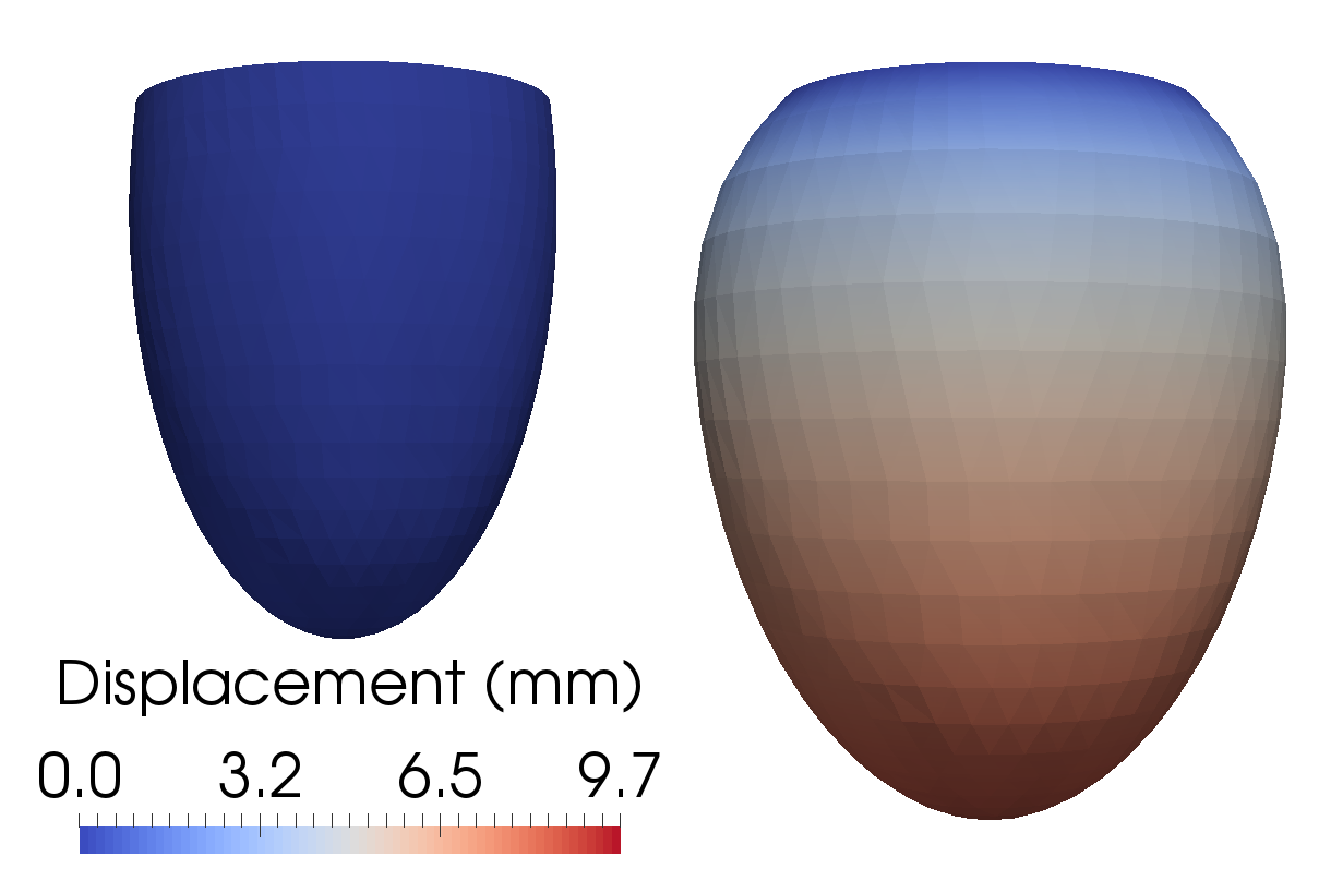
(a) The unloaded (left) and loaded (right) configurations.

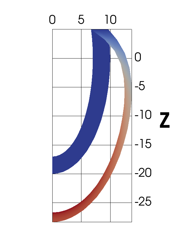
(b) A sliced view of both configurations.

Figure 3: Displacement at the final loading step, $p=10$ kPa, of the idealized left ventricle.

			Final Apex Location ($z$, mm)
Mesh Size ($\mu$m)	DOF($\mathbf{u}$)	DOF($p$)	Endocardium	Epicardium
2000	6264	362	-26.85	-28.09
1000	63630	3084	-26.68	-28.34
500	475176	21504	-26.67	-28.33
300	2156805	94622	-26.67	-28.33

Table 1: Convergence study results for the ellipsoid problem. P2-P1 elements were used for all simulations. Endocardial and epicardial apex locations are in agreement with Figure 6 in Land et al. [14].

4 Impact and Conclusions

Benefits of FEniCS Mechanics stem from the fact that it is built on top of the FEniCS Project. Hence no additional installations are required other than the optional CBC-Block application, as mentioned in Section 2.1. FEniCS provides an interface to state-of-the-art linear solvers and preconditioners from freely available third-party libraries, e.g. PETSc, HYPRE, and Eigen. This is an advantage not found in many other open source projects, which depend on their own solver packages. Another main benefit of using FEniCS as the backbone is the inheritance of parallelization. Problems formulated with FEniCS Mechanics can be run in parallel, given that FEniCS is installed with MPI support. Due to its design as a Python dictionary the simulations are executed in a similar fashion on a high-performance computing cluster as on a regular desktop computer.

A key benefit of FEniCS Mechanics, which distinguishes it from standalone FEniCS, is the reduction of programming skills and theoretical numerical knowledge required from the user. Several common material models have been implemented and the current problem classes span a wide range of possible applications. Altogether, this facilitates access to experimentation and comparison of solutions from differing problem definitions. The names of dictionary keys and values have been chosen to be intuitive to minimize the gap between a user and the simulation they wish to run. This also enables FEniCS Mechanics to raise exceptions when erroneous or inconsistent values are provided by a user, as described in Section 2.2.

While a simplistic interface was maintained in FEniCS Mechanics to facilitate running simulations, advanced users can take full advantage of additional tools provided by the FEniCS Project for altering problem definitions, such as, but not limited to, providing their own constitutive equations for rapid prototyping. Advanced users can also more finely tune the solver and preconditioner parameters used, and perform post-processing tasks within the same script.

Required Metadata

Current code version

Nr.	Code metadata description	Please fill in this column
C1	Current code version	v1.0
C2	Permanent link to code/repository used for this code version	https://gitlab.com/ShaddenLab/fenicsmechanics
C3	Legal Code License	BSD-3-clause
C4	Code versioning system used	git
C5	Software code languages, tools, and services used	Python
C6	Compilation requirements, operating environments & dependencies	FEniCS Project, Version 2016.1.0 and up
C7	If available Link to developer documentation/manual	https://shaddenlab.gitlab.io/fenicsmechanics
C8	Support email for questions	miguelr@berkeley.edu

Table 2: Code metadata

References

- [1] The deal.ii finite element library. URL https://dealii.org.
- [2] Fenics project. https://fenicsproject.org/. Accessed: Nov. 2016.
- [3] Freefem++. URL http://www.freefem.org.
- Abaqus [2018] Abaqus. version 2018. Simulia, Providence, Rhode Island, 2018. URL https://www.3ds.com/products-services/simulia/products/abaqus/.
- ADINA [2018] ADINA. version 9.4.3. ADINA R&D Inc., Watertown, Massachusetts, 2018. URL http://www.adina.com/.
- ANSYS [2018] ANSYS. version 19.2. ANSYS, Inc., Canonsburg, Pennsylvania, 2018. URL https://www.ansys.com/.
- COMSOL Multiphysics [2018] COMSOL Multiphysics. version 5.3. COMSOL AB, Stockholm, Sweden, 2018. URL https://www.comsol.com/.
- Costa et al. [2001] Kevin D. Costa, Jeffrey W. Holmes, and Andrew D. Mcculloch. Modelling cardiac mechanical properties in three dimensions. Philosophical Transactions of the Royal Society A: Mathematical, Physical and Engineering Sciences, 359(1783):1233–1250, 2001. doi: 10.1098/rsta.2001.0828.
- Demiray [1972] Hilmi Demiray. A note on the elasticity of soft biological tissues. Journal of Biomechanics, 5(3):309–311, 1972. doi: 10.1016/0021-9290(72)90047-4.
- Guccione et al. [1995] Julius M. Guccione, Kevin D. Costa, and Andrew D. Mcculloch. Finite element stress analysis of left ventricular mechanics in the beating dog heart. Journal of Biomechanics, 28(10):1167–1177, 1995. doi: 10.1016/0021-9290(94)00174-3.
- Holzapfel and Ogden [2009] Gerhard A. Holzapfel and Ray W. Ogden. Constitutive modelling of passive myocardium: a structurally based framework for material characterization. Philosophical Transactions of the Royal Society A: Mathematical, Physical and Engineering Sciences, 367(1902):3445–3475, Mar 2009. doi: 10.1098/rsta.2009.0091.
- Humphrey [1995] Jay D. Humphrey. Mechanics of the arterial wall: Review and directions. Critical Reviews in Biomedical Engineering, 23(1-2):1–162, 1995. doi: 10.1615/critrevbiomedeng.v23.i1-2.10.
- [13] K. Ladutenko. Fea-compare. URL https://github.com/kostyfisik/FEA-compare.
- Land et al. [2015] Sander Land, Viatcheslav Gurev, Sander Arens, Christoph M. Augustin, Lukas Baron, Robert Blake, Chris Bradley, Sebastian Castro, Andrew Crozier, Marco Favino, and et al. Verification of cardiac mechanics software: benchmark problems and solutions for testing active and passive material behaviour. Proceedings of the Royal Society A: Mathematical, Physical and Engineering Science, 471(2184):20150641, Aug 2015. doi: 10.1098/rspa.2015.0641.
- Logg et al. [2016] Anders Logg, Kent-Andre Mardal, and Garth Wells. Automated Solution of Differential Equations by the Finite Element Method: The FEniCS Book. Springer Berlin, 2016.
- [16] Wikipedia. List of finite element software packages. URL https://en.wikipedia.org/wiki/List_of_finite_element_software_packages.