Self-avoiding walks and connective constants in clustered scale-free networks

Abstract

Various types of walks on complex networks have been used in recent years to model search and navigation in several kinds of systems, with particular emphasis on random walks. This gives valuable information on network properties, but self-avoiding walks (SAWs) may be more suitable than unrestricted random walks to study long-distance characteristics of complex systems. Here we study SAWs in clustered scale-free networks, characterized by a degree distribution of the form $P(k)\sim k^{-\gamma}$ for large $k$. Clustering is introduced in these networks by inserting three-node loops (triangles). The long-distance behavior of SAWs gives us information on asymptotic characteristics of such networks. The number of self-avoiding walks, $a_{n}$, has been obtained by direct enumeration, allowing us to determine the connective constant $\mu$ of these networks as the large-$n$ limit of the ratio $a_{n}/a_{n-1}$. An analytical approach is presented to account for the results derived from walk enumeration, and both methods give results agreeing with each other. In general, the average number of SAWs $a_{n}$ is larger for clustered networks than for unclustered ones with the same degree distribution. The asymptotic limit of the connective constant for large system size $N$ depends on the exponent $\gamma$ of the degree distribution: For $\gamma>3$, $\mu$ converges to a finite value as $N\to\infty$; for $\gamma=3$, the size-dependent $\mu_{N}$ diverges as $\ln N$, and for $\gamma<3$ we have $\mu_{N}\sim N^{(3-\gamma)/2}$.

I Introduction

In last decades, research in various fields has shown evidence that many types of real-life systems can be described in terms of networks, where nodes represent typical system units and edges correspond to interactions between connected pairs of units. Such topological characterization has been applied to describe natural and artificial systems, and is used at present to analyze processes occurring in real systems (social, economic, technological, biological) Dorogovtsev and Mendes (2003); Cohen and Havlin (2010); Albert and Barabási (2002); Strogatz (2001); von Ferber and Holovatch (2013).

Several kinds of theoretical and experimental techniques have been employed to study and characterize a diversity of networks da F. Costa et al. (2007); Newman (2010). Various of these methods aim at studying dynamical processes, such as spread of infections Moore and Newman (2000); Kuperman and Abramson (2001); Hebert-Dufresne et al. (2010); Bauer and Lizier (2012); Liu et al. (2017), signal propagation Watts and Strogatz (1998); Herrero (2002), and random spreading of information and opinion Pandit and Amritkar (2001); Moreno et al. (2004); Candia (2007). The network structure plays an important role in these processes, as has been shown by using stochastic dynamics and random walks Jasch and Blumen (2001); Almaas et al. (2003); Newman (2003); Noh and Rieger (2004); Costa and Travieso (2007); Lopez Millan et al. (2012).

It turns out that many systems can be described by so-called scale-free (SF) networks, displaying a power-law distribution of degrees. In an SF network the degree distribution $P_{\rm sf}(k)$, where $k$ is the number of links connected to a node, has a power-law decay $P_{\rm sf}(k)\sim k^{-\gamma}$. Networks displaying such a degree distribution have been found in both natural and artificial systems, e.g., internet Siganos et al. (2003), world-wide web Albert et al. (1999), social systems Newman (2001), and protein interactions Jeong et al. (2001). In these networks, the exponent $\gamma$ describing the distribution $P_{\rm sf}(k)$ has been usually found in the range $2<\gamma<3$ Dorogovtsev and Mendes (2003); Goh et al. (2002). SF networks have been used to study statistical physics problems, as avalanche dynamics Goh et al. (2003), percolation Radicchi and Fortunato (2009), and cooperative phenomena Dorogovtsev et al. (2002); Herrero (2004); Bartolozzi et al. (2006); Dorogovtsev et al. (2008); Herrero (2009); Dommers et al. (2010); Ostilli et al. (2011).

Self-avoiding walks (SAWs) can be more effective than unrestricted random walks in exploring networks, since they are not allowed to return to sites already visited in the same walk Kim et al. (2016); Tishby et al. (2016). This property has been used to define local search strategies in scale-free networks Adamic et al. (2001). SAWs have been employed with various purposes, such as modeling structural and dynamical aspects of polymers de Gennes (1979); Orlandini and Whittington (2007); Beaton et al. (2012); Guttmann et al. (2014), conformation of DNA molecules Maier and Radler (1999); Witz et al. (2008), characterization of complex crystal structures Herrero (1995, 2014), and analysis of critical phenomena in lattice models Kremer et al. (1982); Clisby (2010); Guttmann and Jacobsen (2013). In the context of complex networks, several features of SAWs have been studied in small-world Herrero and Saboyá (2003), scale-free Herrero (2005a), and fractal networks Hotta (2014); Fricke and Janke (2014).

The asymptotic properties of SAWs in regular and complex networks are usually studied in connection with the so-called connective constant or long-distance effective connectivity, which quantifies the increase in the number of SAWs at long distances Rapaport (1985); Privman et al. (1991). For SF networks, in particular, this has allowed to distinguish different regimes depending on the exponent $\gamma$ of the distribution $P_{\rm sf}(k)$ Herrero (2005a). One can also consider kinetic-growth self-avoiding walks on complex networks, to study the influence of attrition on the maximum length of the paths Herrero (2005b, 2007), but this kind of walks will not be addressed here.

Many real-life networks include clustering, i.e., the probability of finding loops of small size is larger than in random networks. This has been in particular quantified by the so-called clustering coefficient, which measures the likelihood of three-node loops (triangles) in a network Newman (2010). The relevance of loops for different aspects of networks is now generally recognized, and several models of clustered networks have been defined and analyzed by several research groups Holme and Kim (2002); Klemm and Eguiluz (2002); Serrano and Boguñá (2005); Klaise and Johnson (2018); Lopez et al. (2018). In recent years, it has been shown that generalized random graphs can be generated incorporating clustering in such a way that exact formulas can be derived for many of their properties Newman (2009); Miller (2009); Heath and Parikh (2011). This includes the study of physical problems such as critical phenomena in SF networks, e.g. the Ising model Herrero (2015). For an exponent $\gamma\leq 3$ it was found that clustered and unclustered networks with the same size and degree distribution $P(k)$ have different paramagnetic-ferromagnetic transition temperature $T_{c}$, what indicates that clustering favors ferromagnetic correlations and causes an increase in $T_{c}$. Other works on clustered networks have addressed different questions, as robustness Huang et al. (2013), bond percolation Gleeson (2009); Gleeson et al. (2010); Radicchi and Castellano (2016), and spread of diseases Molina and Stone (2012); Wang et al. (2012).

Here we study long-range properties of SAWs in clustered SF networks. We pose the question whether clustering significantly changes the properties of SAWs in this kind of networks. This is particularly interesting for the long-distance behavior of SAWs, which is expected to depend on network characteristics such as cluster concentration and decay of the degree distribution for large degree (exponent $\gamma$ for SF networks). Thus, we focus on the influence of introducing clusters (here triangles) upon the asymptotic limits of SAWs and connective constants. The average number of walks for a given length $n$ is calculated by an iterative procedure, and the results are compared with those obtained from direct enumeration in simulated networks. Both methods yield results which agree with each other in the different regions defined by the exponent $\gamma$ and for a wide range of cluster densities. Comparing results for clustered and unclustered networks with the same degree distribution, we find for large networks with $\gamma>3$ that the long-distance behavior of SAWs is not affected by clustering. On the other hand, clustering changes the connective constants derived from SAWs for networks with $\gamma\leq 3$.

The paper is organized as follows. In Sec. II we describe the clustered SF networks studied here. In Sec. III we present some generalities on SAWs and its application to unclustered scale-free networks. In Sec. IV we introduce an analytical method employed to calculate the number of SAWs in clustered networks, and in Sec. V we compare results of this analytical procedure with those obtained by directly enumerating SAWs in simulated networks. The paper closes with the conclusions in Sec. VI.

II Description of the networks

II.1 Networks construction

We study here clustered networks with a degree distribution $P(k)$, which for large degree $k$ follows a power-law $P_{\rm sf}(k)\sim k^{-\gamma}$. The exponent controlling the decay of the distribution is taken as $\gamma>2$, so that the mean degree $\langle k\rangle$ remains finite in the large-size limit. Clustering is introduced by including triangles into the networks, i.e., triads of connected nodes. One can consider other types of polygons (squares, pentagons, …) to study their effect on the properties of clustered networks, but we take triangles as they are expected to give rise to stronger correlations between entities defined on network sites Herrero (2015). The analytical method described here to study SAWs in the presence of triangles can be easily extended to other types of motifs.

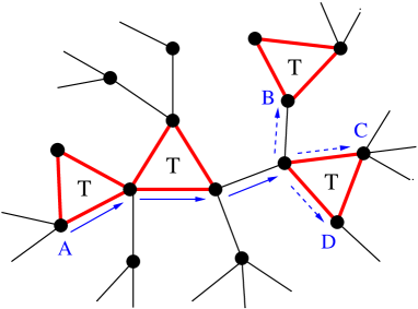
Figure 1: Schematic representation of a typical network considered in this work, for which one separately specifies the number of single edges and triangles (bold red edges) attached to each node. Triangles are indicated as T. Arrows indicate a possible SAW starting from node A. For the fourth step ($n=4$), there are three available edges (one $s$-link and two $t$-links) reaching nodes B, C, and D.

Our networks are generated by using the procedure described by Newman Newman (2009), where the number of single edges and the number of triangles are independently defined. A method like this permits us to manage generalized random graphs, which incorporate clustering in a rather simple manner, thus allowing one to analytically study various properties of the resulting networks Newman (2009). Given a network, we call $N$ the number of nodes, $t_{i}$ the number of triangles of which node $i$ is a vertex, and $s_{i}$ the number of single links not included in triangles ($i=1,...,N$). This means that, for the purpose of network construction, edges within triangles are considered apart from single links. Then, a single link can be regarded as an element connecting two nodes and a triangle as a network component joining together three nodes. Thus, the degree $k_{i}$ of node $i$ is given by $k_{i}=s_{i}+2\,t_{i}$, since each triangle connects it to two other nodes. A schematic plot of this kind of networks is displayed in Fig. 1, where triangles are marked as T. In this figure, single links appear as black lines and edges belonging to triangles are depicted as bold red lines. For clarity of the presentation below, both kinds of edges will be denoted $s$-links and $t$-links, respectively.

The networks are built in two steps. In the first one, we introduce the edges by connecting pairs of nodes. We ascribe to each node $i$ a random integer $s_{i}$, which will be the number of outgoing links (stubs) from this node. The numbers $\{s_{i}\}_{i=1}^{N}$ are picked up from the probability distribution $P_{\rm sf}(s)\sim s^{-\gamma}$, assuming that $s_{i}\geq k_{0}$, the minimum allowed degree Newman (2005). This gives a total number of stubs $K=\sum_{i=1}^{N}s_{i}$, which we impose to be an even integer. Once the numbers $s_{i}$ are defined, we connect stubs at random (giving a total of $L=K/2$ connections), with the conditions: (i) no two nodes can have more than one edge connecting them (no multiedges), and (ii) no node can be connected by a link to itself (no self-edges). Networks fulfilling these conditions are usually called simple networks or simple graphs Newman (2010).

In a second step we incorporate $N_{\Delta}$ triangles into the considered network. $N_{\Delta}$ is defined by the parameter $\nu$, the mean number of triangles in which a node is included, $N_{\Delta}=\frac{1}{3}N\nu$. The number of triangles associated to each node is taken from a Poisson distribution $Q(t)={\rm e}^{-\nu}\nu^{t}/t!$. This gives us $t_{i}$ corners corresponding to node $i$, and the total number is $T=\sum_{i=1}^{N}t_{i}=3N_{\Delta}$. For consistency, $T$ has to be a multiple of 3. Then, we randomly choose triads of corners to form triangles, avoiding multiple and self-edges as in conditions (i) and (ii) in the previous paragraph.

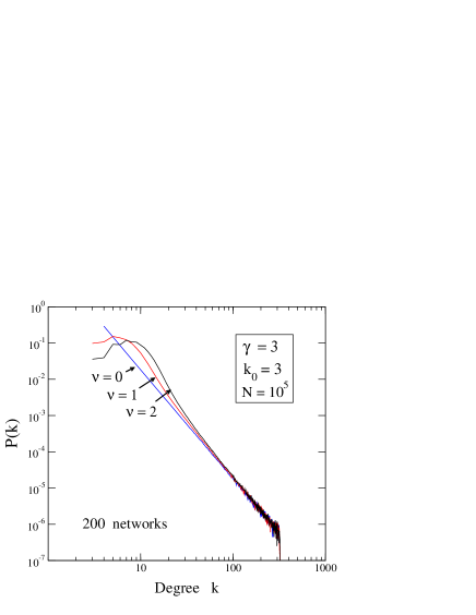
Figure 2: Probability density $P(k)$ as a function of the degree $k$ for networks with $\gamma=3$, minimum degree $k_{0}$ = 3, and $N=10^{5}$ nodes. The displayed data are an average over 200 network realizations for each value of the parameter $\nu$ = 0, 1, and 2.

It is known that long-tailed distributions including nodes with very large degree may display undesired correlations between the degrees of adjacent nodes, especially for exponents $\gamma<3$ Catanzaro et al. (2005). For this reason we have introduced in the networks considered here a maximum-degree cutoff $s_{\rm cut}=\sqrt{N}$, which avoids such correlations (see Sec. II.B) Catanzaro et al. (2005); Herrero (2015). This restriction is in fact only effective for $\gamma<3$, as explained below.

The degree distribution $P(k)$ obtained for clustered networks generated by following the procedure presented above is shown in Fig. 2. In this figure, we display $P(k)$ for networks with $N=10^{5}$ nodes, $\gamma=3$ and $k_{0}=3$. Shown are results for three values of the triangle density: $\nu$ = 0, 1, and 2, corresponding in each case to an average over 200 network realizations. One observes that increasing the value of $\nu$ causes clear changes in $P(k)$ for small $k$ values, with respect to the degree distribution for $\nu=0$. For large degrees, however, the distribution follows a dependence $P_{\rm sf}(k)\sim k^{-\gamma}$ characteristic of scale-free networks with $\gamma=3$. This could be expected from the fact that the Poisson distribution $Q(t)$ associated to the triangles has a fast exponential-like decay for large $t$.

In summary, our networks are defined by the following parameters: $N$ (number of nodes), $k_{0}$ (minimum degree), $\gamma$ (exponent controlling the distribution of single edges, $P_{\rm sf}(s)$), and $\nu$ (density of triangles). For the numerical simulations we have generated networks with several values of these parameters. For each set ($N$, $k_{0}$, $\gamma$, $\nu$), we considered different network realizations, and for a given network we selected at random the starting nodes for the SAWs. For each considered parameter set, the total number of generated SAWs amounted to about $2\times 10^{6}$. All networks considered here contain a single component, i.e. any node in a network can be reached from any other node by traveling through a finite number of links.

For comparison with the results obtained for clustered networks, we have also generated networks with the same degree distribution $P(k)$ than the clustered ones, but without explicitly including triangles. This means that these networks are built up from the degree sequence $\{k_{i}\}_{i=1,...,N}$ given by $k_{i}=s_{i}+2t_{i}$, but randomly connecting the $k_{i}$ outgoing links (stubs) for each node $i$ as indicated above for $s$-links. This corresponds to the so-called configuration model Newman (2010).

II.2 Mean values $\langle k\rangle$ and $\langle k^{2}\rangle$

Important characteristics of the considered networks, which will be used below in our calculations, are the mean values $\langle k\rangle$ and $\langle k^{2}\rangle$. For scale-free networks with $\nu=0$ (no clustering), the average degree is given by

$$\langle s\rangle_{\infty}=\sum_{s=k_{0}}^{\infty}s\,P_{\rm sf}(s)\approx k_{0}\,\frac{\gamma-1}{\gamma-2}\;,$$ (1)

where the expression on the right has been obtained by replacing the sum by an integral, which is justified for large $N$. For our networks including triangles ($\nu>0$), we have $k_{i}=s_{i}+2t_{i}$, and

$$\langle k\rangle_{\infty}=\langle s\rangle_{\infty}+2\,\nu\approx k_{0}\,\frac{\gamma-1}{\gamma-2}+2\,\nu\;.$$ (2)

For clarity of the presentation we write $\langle s\rangle$ to indicate an average value for unclustered SF networks (configuration model), i.e. consisting of $s$-links. We write $\langle k\rangle$ in the general case, which includes clustered networks. Moreover, the subscripts $N$ and $\infty$ refer to networks of size $N$ and to the infinite-size limit (when it exists), respectively. When no subscript appears, we understand that it refers to a general case, without mention to the system size.

For finite networks, a size effect appears in the mean degree, as a consequence of the effective cutoff $k_{\rm cut}$ appearing in the degree distribution. In fact, for a given network of size $N$ one has Dorogovtsev et al. (2002); Iglói and Turban (2002)

$$\sum_{k_{\rm cut}}^{\infty}P_{\rm sf}(s)=\frac{c}{N}\;,$$ (3)

where $c$ is a constant on the order of unity. This yields for $k_{\rm cut}\gg k_{0}$ Herrero (2015):

$$k_{\rm cut}\approx k_{0}\left(\frac{N}{c}\right)^{\frac{1}{\gamma-1}}\,,$$ (4)

so that $k_{\rm cut}\sim\,N^{1/(\gamma-1)}$, as in Dorogovtsev et al. (2002); Iglói and Turban (2002). From Eq. (4), one obtains for finite scale-free networks Herrero (2015):

$$\langle s\rangle_{N}\approx\langle s\rangle_{\infty}\left[1-\left(\frac{c}{N}\right)^{\frac{\gamma-2}{\gamma-1}}+{\cal O}\left(\frac{1}{N}\right)\right]\;.$$ (5)

For the mean value $\langle s^{2}\rangle$, the size dependence and its large-size behavior change with the exponent $\gamma$. For SF networks with $\gamma>3$, the dependence of $\langle s^{2}\rangle$ on $N$ is similar to that of $\langle s\rangle$, namely Herrero (2015) :

$$\langle s^{2}\rangle_{N}\approx\langle s^{2}\rangle_{\infty}\left[1-\left(\frac{c}{N}\right)^{\frac{\gamma-3}{\gamma-1}}+{\cal O}\left(\frac{1}{N}\right)\right]\;,$$ (6)

with $\langle s^{2}\rangle_{\infty}\approx k_{0}^{2}\,(\gamma-1)/(\gamma-3)$.

For $\gamma=3$, we have

$$\langle s^{2}\rangle_{N}=\sum_{k_{0}}^{k_{\rm cut}}s^{2}P_{\rm sf}(s)\approx\frac{2}{k_{0}^{-2}-k_{\rm cut}^{-2}}\,\ln\frac{k_{\rm cut}}{k_{0}}\;,$$ (7)

and using Eq. (4) we find for $k_{\rm cut}\gg k_{0}$:

$$\langle s^{2}\rangle_{N}=k_{0}^{2}\,\ln N+{\cal O}(1)\;.$$ (8)

For SF networks with an exponent $\gamma<3$, Catanzaro et al. Catanzaro et al. (2005) found appreciable correlations between degrees of adjacent nodes when no multiple and self-edges are allowed. These degree correlations can be avoided by introducing a cutoff $k_{\rm cut}\sim N^{1/2}$, as indicated above. Thus, for $\gamma<3$ we generate here networks with a cutoff $k_{\rm cut}=N^{1/2}$. Note that for $\gamma>3$ the cutoff derived above from the condition given in Eq. (3) is more restrictive than putting $k_{\rm cut}=N^{1/2}$, so that in this case the effective cutoff is given by Eq. (4). Then, for finite networks with $\gamma<3$ the mean values $\langle s\rangle_{N}$ and $\langle s^{2}\rangle_{N}$ are given by:

$$\langle s\rangle_{N}\approx\langle s\rangle_{\infty}\left[1-\left(\frac{k_{0}}{\sqrt{N}}\right)^{\gamma-2}\right]\;,$$ (9)

and

$$\langle s^{2}\rangle_{N}\approx k_{0}^{2}\,\frac{\gamma-1}{3-\gamma}\left(\frac{\sqrt{N}}{k_{0}}\right)^{3-\gamma}\;.$$ (10)

For clustered SF networks with a triangle density $\nu>0$, the average value $\langle k^{2}\rangle$ is given by

$$\langle k^{2}\rangle=\langle(s+2t)^{2}\rangle=\langle s^{2}\rangle+4\langle s\rangle\langle t\rangle+4\langle t^{2}\rangle\;,$$ (11)

where we have used the fact that $\langle s\,t\rangle=\langle s\rangle\langle t\rangle$, since variables $s$ and $t$ are independent for the way of building up these networks. Then, for clustered networks with $\gamma>3$, we have in the large-size limit:

$$\langle k^{2}\rangle_{\infty}\approx k_{0}^{2}\,\frac{\gamma-1}{\gamma-3}+4\,k_{0}\,\nu\,\frac{\gamma-1}{\gamma-2}+4\,\nu\,(\nu+1)\,,$$ (12)

where $\nu$ and $\nu\,(\nu+1)$ are the average values $\langle t\rangle$ and $\langle t^{2}\rangle$ corresponding to the Poisson distribution of triangles $Q(t)$. For scale-free networks with $\gamma\leq 3$ one can write expressions for $\langle k^{2}\rangle_{N}$ derived from Eq. (11) by using the corresponding formulas for $\langle s\rangle_{N}$ and $\langle s^{2}\rangle_{N}$ given above.

II.3 Clustering coefficient

The clustering coefficient $C$ is usually defined for complex networks as the ratio Newman (2010, 2009); Yoon et al. (2011)

$$C=\frac{3N_{\Delta}}{N_{3}}\;,$$ (13)

where $N_{\Delta}$ is the number of triangles and $N_{3}$ is the number of connected triplets. Here a connected triplet means three nodes $n_{1}n_{2}n_{3}$ with links ($n_{1},n_{2}$) and ($n_{2},n_{3}$), and $N_{3}$ is given by

$$N_{3}=N\sum_{k}\frac{k(k-1)}{2}P(k)=\frac{1}{2}N\left(\langle k^{2}\rangle-\langle k\rangle\right)\;.$$ (14)

Taking into account that the triangle density in our clustered networks is related to the number of triangles $N_{\Delta}$ by the expression $N_{\Delta}=N\nu/3$, we have

$$C=\frac{2\nu}{\langle k^{2}\rangle-\langle k\rangle}\;.$$ (15)

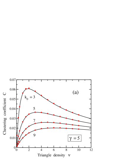
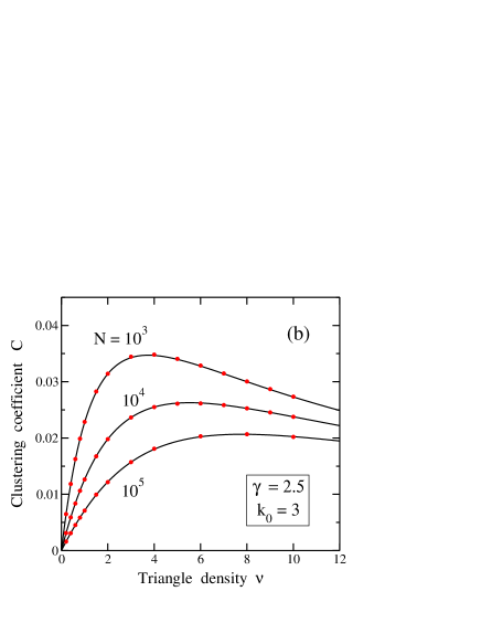
Figure 3: Clustering coefficient $C$ as a function of the triangle density $\nu$ for clustered scale-free networks. (a) $\gamma=5$ and various values of the minimum degree $k_{0}$. From top to bottom, $k_{0}$ = 3, 5, 7, and 9. Solid circles represent results derived from clustered networks with $N=10^{5}$ nodes. Solid lines were analytically derived in the limit $N\to\infty$ by using the expressions given in the text. (b) $\gamma=2.5$ and three different network sizes: $N=10^{3}$, $10^{4}$, and $10^{5}$. Solid lines were calculated by using the formulas for $\langle s\rangle_{N}$ and $\langle s^{2}\rangle_{N}$ given in Sec. II.B for $\gamma<3$.

Note that in our clustered networks it is possible for single edges to form triangles. The average number $N_{\Delta}^{\rm rd}$ of such triangles is given by Newman (2010)

$$N_{\Delta}^{\rm rd}=\frac{1}{6}\left(\frac{\langle k^{2}\rangle}{\langle k\rangle}-1\right)^{3}\;.$$ (16)

This mean value is small for scale-free networks with large $\gamma$, and rises as $\gamma$ decreases. The density of these triangles, $N_{\Delta}^{\rm rd}/N$, vanishes in the thermodynamic limit for $\gamma>7/3$, and for $\gamma<7/3$ this ratio scales as a power of $N$ with exponent $(7-3\gamma)/2$. Calling $\nu_{0}$ the mean number of randomly-generated triangles per node, we have

$$\nu_{0}=\frac{3N_{\Delta}^{\rm rd}}{N}\;,$$ (17)

which rapidly converges to zero for large $N$ for the network parameters considered here. For the minimum value of $\gamma$ studied here, $\gamma=2.5$, we have $\nu_{0}\approx\frac{1}{2}k_{0}^{3/2}N^{-1/4}$, i.e., $\nu_{0}\approx 0.15$ for $k_{0}=3$ and $N=10^{5}$. With these parameters and $\gamma=3$, we find $\nu_{0}\approx 0.02$.

In Fig. 3 we show the clustering coefficient $C$ as a function of the triangle density $\nu$ for clustered scale-free networks. Panel (a) corresponds to $\gamma=5$ and several values of the minimum degree $k_{0}$. Solid symbols were derived from simulations of networks with $N=10^{5}$, and the lines were obtained by using Eq. (15) with the mean values $\langle k\rangle_{\infty}$ and $\langle k^{2}\rangle_{\infty}$ given in Sec. II.B, Eqs. (2) and (12). Small differences between both sets of results are due to the finite size of the simulated networks. For small triangle density $\nu$, the clustering coefficient increases for rising $\nu$ and reaches a maximum, which is more pronounced for smaller $k_{0}$. For a given triangle density $\nu$, $C$ decreases for increasing minimum degree $k_{0}$, as a consequence of the rise in the difference $\langle k^{2}\rangle-\langle k\rangle$ which appears in the denominator of Eq. (15).

In Fig. 3(b), $C$ is plotted vs $\nu$ for scale-free networks with $\gamma=2.5$ and three system sizes: $N=10^{3}$, $10^{4}$, and $10^{5}$. Here one observes a clear dependence of $C$ on $N$, with the clustering coefficient decreasing when rising $N$ for a given triangle density $\nu$. For large $\nu$, one finds a slow decrease in $C$ for increasing $\nu$, with the different curves approaching one to the other.

III Generalities on self-avoiding walks

A self-avoiding walk is defined as a walk along the edges of a network which cannot intersect itself. The walk is restricted to moving to a nearest-neighbor node in each step, and the self-avoiding condition restricts the walk to visit only nodes which have not been occupied earlier in the same walk. Here we do not consider SAWs as kinetically-grown walks in a dynamical process, and just calculate (i.e., count) the number of possible SAWs starting from a given node in a given network. This means that all those SAWs have the same weight for calculating ensemble averages, e.g. the connective constant discussed below. This is not the case of kinetically-grown SAWs, for which the weight is in general not uniform Herrero (2005a, b). The number of SAWs of length $n$ in complex networks depends in general on the considered starting node, however some properties such as the connective constant of a given network are independent of the initial node (see below). In the following we will call $a_{n}$ the average number of SAWs of length $n$, i.e. the mean value obtained by averaging over the network sites and over different network realizations (for a given set of parameters $N$, $k_{0}$, $\gamma$, and $\nu$).

Self-avoiding walks have been traditionally studied on regular lattices. In this case, it is known that the number of SAWs increases for large $n$ as $a_{n}\sim n^{\Gamma-1}\mu^{n}$, where $\Gamma$ is a critical exponent which depends on the lattice dimension $D$ and $\mu$ is the connective constant or effective coordination number of the considered lattice Rapaport (1985). For $D>4$ one has $\Gamma=1$ Privman et al. (1991); Sokal (1995). For a lattice with connectivity $k_{0}$, the connective constant verifies $\mu\leq k_{0}-1$, and can be obtained from the large-$n$ limit

$$\mu=\lim_{n\to\infty}\frac{a_{n}}{a_{n-1}}\hskip 8.53581pt.$$ (18)

This parameter depends on the particular topology of each lattice, and has been calculated very accurately for two- and three-dimensional lattices Sokal (1995).

For complex networks in general the situation is rather different than in the case of regular lattices in low dimensions. This is particularly clear for random networks, which are locally tree-like and do not display the so-called attrition of SAWs caused by the presence of small-size loops of connected nodes. A simple case of network without loops is a Bethe lattice (or Cayley tree) with fixed connectivity $k_{0}$, for which the number of SAWs is given by $a_{n}^{BL}=k_{0}(k_{0}-1)^{n-1}$, and then $\mu_{BL}=k_{0}-1$. For Erdös-Rényi random networks Bollobás (1998) with poissonian distribution of degrees, one has $a_{n}^{\rm ER}=\langle k\rangle^{n}$ Herrero and Saboyá (2003), and then the connective constant is $\mu^{\rm ER}=\langle k\rangle$.

For generalized random networks (configuration model), one has Herrero (2005a)

$$a_{n}=\langle k\rangle\left(\frac{\langle k^{2}\rangle}{\langle k\rangle}-1\right)^{n-1}\;.$$ (19)

In this expression, the ratio $\langle k^{2}\rangle/\langle k\rangle$ is the average degree of a randomly-chosen end node of a randomly selected edge Dorogovtsev and Mendes (2002); Newman (2010). The term $-1$ in Eq. (19) introduces the self-avoiding condition. Thus, the connective constant $\mu$ for random networks is given by

$$\mu=\frac{\langle k^{2}\rangle}{\langle k\rangle}-1\;.$$ (20)

Note that the expression given above for $\mu$ in Erdös-Rényi networks is a particular case of Eq. (20), since for these networks one has $\langle k^{2}\rangle/\langle k\rangle=\langle k\rangle+1$. As indicated above, the number of SAWs on regular lattices scales for large $n$ as $a_{n}\sim n^{\Gamma-1}\mu^{n}$ Privman et al. (1991); Sokal (1995). For unclustered SF networks one has $a_{n}\sim\mu^{n}$, indicating that $\Gamma=1$, the same exponent as for regular lattices in $D>4$.

For scale-free networks with $\gamma>3$, both $\langle k\rangle$ and $\langle k^{2}\rangle$ converge to finite values in the large-system limit. Thus, for unclustered networks (triangle density $\nu=0$) one can approximate the average values in Eq. (20) by those given in Sec. III.A for $\langle k\rangle_{\infty}$ and $\langle k^{2}\rangle_{\infty}$, yielding

$$\mu\approx k_{0}\;\frac{\gamma-2}{\gamma-3}-1\;.$$ (21)

For large $\gamma$ we recover the connective constant corresponding to random regular networks ($k_{i}=k_{0}$ for all nodes), $\mu=k_{0}-1$, as for the Bethe lattice commented above.

For $\gamma\leq 3$ the mean value $\langle k^{2}\rangle$ diverges for $N\to\infty$, and the connective constant $\mu$ defined in Eq. (18) also diverges in the large-size limit Herrero (2005a). In this case we will consider a size-dependent connective constant $\mu_{N}$ defined as

$$\mu_{N}=\frac{\langle k^{2}\rangle_{N}}{\langle k\rangle_{N}}-1\;.$$ (22)

Then, for unclustered SF networks with $\gamma=3$ and $\nu=0$, one has

$$\mu_{N}\approx\frac{1}{2}k_{0}\ln N\;.$$ (23)

For $2<\gamma<3$ and $\nu=0$, $\mu_{N}$ behaves for large unclustered networks as

$$\mu_{N}\approx k_{0}\frac{\gamma-2}{3-\gamma}\left(\frac{\sqrt{N}}{k_{0}}\right)^{3-\gamma}\;.$$ (24)

We emphasize that the expressions given in Eqs. (20) and (22) for the connective constants $\mu$ and $\mu_{N}$, as well as those presented in this Section for SF networks with different values of $\gamma$, are valid for unclustered networks (configuration model). For clustered networks (in our case, triangle density $\nu>0$), those expressions are not valid because triangles introduce correlations in the degrees of adjacent nodes. In this case, one has to implement a different procedure to calculate the ratio $a_{n}/a_{n-1}$ necessary to obtain the connective constant of clustered networks.

IV Self-avoiding walks: analytical procedure

In this section we present an analytical method to calculate the connective constant in clustered scale-free networks, based on an iterative procedure to obtain the average number of walks $a_{n}$ for increasing walk length $n$. The ratio $a_{n}/a_{n-1}$ derived from this method converges fast for the networks studied here (parameter $\gamma>2$). In this procedure we take advantage of the fact that the number of links $s_{i}$ and $t_{i}$ connected to a node $i$ are independent.

The number of $n$-step self-avoiding walks, $a_{n}$, can be written as

$$a_{n}=b_{n}+c_{n}\;,$$ (25)

where $b_{n}$ and $c_{n}$ are the number of walks for which step $n$ proceeds via an $s$-link or a $t$-link, respectively (no matter the kind of links employed in the previous steps). Note that the quantities $a_{n}$, $b_{n}$, and $c_{n}$, are average values for all possible starting nodes in the considered networks. To simplify the notation, we will call $\alpha=2\nu$, i.e., $\alpha$ is the average number of $t$-links connected to a node, $\alpha=2\langle t\rangle$. Moreover, we will call

$$z=\langle s\rangle,\hskip 28.45274ptr=\frac{\langle s^{2}\rangle}{\langle s\rangle}\;.$$ (26)

To obtain $b_{n}$ and $c_{n}$ we will use the iteration formulas (for $n>1$):

$$\left.\begin{array}[]{lll}b_{n}&=&(r-1)\,b_{n-1}+z\,c_{n-1}\\ c_{n}&=&\alpha\,b_{n-1}+(\alpha+1)\,c_{n-1}-\alpha\,a_{n-3}\end{array}\right\}$$ (27)

The initial conditions are: $b_{1}=z$, $c_{1}=\alpha$, $a_{0}=1$, $a_{-1}=0$. In the first equation of (27), $b_{n}$ is calculated from the number of walks $b_{n-1}$ and $c_{n-1}$ of length $n-1$. If step $n-1$ goes on an $s$-link, then the prefactor is $r-1$ to avoid returning on the previous link, as for unclustered SF networks with only $s$-links [see Eq. (19)]. If step $n-1$ proceeds on a $t$-link, then the prefactor of $c_{n-1}$ is $z$ (variables $s$ and $t$ are independent).

To calculate $c_{n}$ in the second equation of (27) we have contributions coming from $b_{n-1}$ and $c_{n-1}$, but there also appears a third term with negative contribution corresponding to the self-avoiding condition, i.e., links associated to closing triangles are not allowed (here we call “closing a triangle” to visit its three edges in three successive steps of a walk). The first two terms on the r.h.s. are obtained from inputs of step $n-1$. If step $n-1$ follows an $s$-link, then the prefactor for $b_{n-1}$ is the mean number of $t$-links per node, i.e., $\alpha$. If step $n-1$ proceeds over a $t$-link, the prefactor for $c_{n-1}$ on the r.h.s. of the second equation is $\alpha+1$. This requires a comment. Remember that in random networks the average degree of a randomly-chosen end node of a randomly selected edge is given by the ratio $\langle k^{2}\rangle/\langle k\rangle$ Dorogovtsev and Mendes (2002); Newman (2010), as indicated above in connection to Eq. (19). Similarly, in our network of triangles, the average number of triangles, $\langle t\rangle^{\prime}$, linked to a randomly-selected end node of a randomly taken $t$-link is given by $\langle t^{2}\rangle/\langle t\rangle$. For the Poisson distribution of triangles we have $\langle t\rangle=\nu$ and $\langle t^{2}\rangle=\nu(\nu+1)$, so that $\langle t\rangle^{\prime}=\nu+1$. Hence, since one $t$-link was already visited in step $n-1$ (this refers to the input associated to $c_{n-1}$), the number of $t$-links available for step $n$ is $2(\nu+1)-1=\alpha+1$ (each triangle includes two available links).

The prefactor for $a_{n-3}$ in the second equation of (27) is the average number of $t$-links corresponding to triangles that close at step $n$. For an SAW of $n-3$ steps, there is an average number of $\nu$ triangles that may close after three more steps in step $n$.

Using both equations in (27), one can derive the connective constant $\mu$ from the asymptotic limit of the ratio $a_{n}/a_{n-1}$. This is presented in Appendix A. We find that $\mu$ can be calculated by solving the system [see Eqs. (39), (42), and (43)]

$$\left.\begin{array}[]{l}\theta\mu^{3}-(\theta\alpha+\theta+\alpha)\mu^{2}+\alpha(1+\theta)=0\\ \mu-z\theta-r+1=0\end{array}\right\}$$ (28)

where $\mu$ and $\theta$ are unknown variables. $\mu$ is the connective constant defined above, and $\theta$ is the asymptotic limit of the ratio $c_{n}/b_{n}$ for large $n$. Both equations can be combined to yield a quartic equation in $\mu$ with coefficients defined from the network parameters $z$, $r$, and $\alpha$. For the networks considered here, this quartic equation has a single positive solution, so that $\mu$ is univocally defined. We note that the initial conditions $b_{1}$ and $c_{1}$ in the system (27) are not relevant for the actual solution of the system. This means that the connective constant derived from (27) is robust, in the sense that putting for $b_{1}$ and $c_{1}$ the values of a particular node $i$ ($s_{i}$ and $t_{i}$) does not change the result for $\mu$, which is a long-range characteristic of each network. Putting mean values for the starting conditions helps to accelerate the convergence of the procedure.

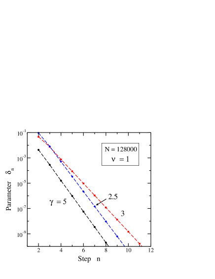
Figure 4: Parameter $\delta_{n}$ as a function of the step number $n$ for clustered scale-free networks with triangle density $\nu=1$, size $N=128,000$ nodes, and minimum degree $k_{0}=3$. Symbols correspond to different values of the exponent $\gamma$: 5 (circles), 3 (squares), and 2.5 (diamonds).

In the case $\nu=0$ (i.e., absence of triangles in unclustered networks, $\alpha=0$), one has, from Eqs. (27), $c_{n}^{\rm un}=0$ for all $n$ and $b_{n}^{\rm un}=(r-1)b_{n-1}^{\rm un}$ with $b_{1}^{\rm un}=\langle s\rangle$ (here the superscript ‘un’ means unclustered). We thus recover the general expression for unclustered networks, Eq. (19), and then $\mu^{\rm un}=\langle s^{2}\rangle/\langle s\rangle-1$.

For $\gamma\leq 3$, we have defined a size-dependent connective constant $\mu_{N}$. In this case, the limits to infinity presented above in this section have no sense. However, the ratios $a_{n}/a_{n-1}$, $b_{n}/b_{n-1}$, and $c_{n}/c_{n-1}$ considered here converge with our present method for relatively low number of steps, $n\ll N$. To analyze the convergence of the ratio $f_{n}=a_{n}/a_{n-1}$, we define the parameter $\delta_{n}=|f_{n}-\mu_{N}|/\mu_{N}$. In Fig. 4 we present in a logarithmic plot the parameter $\delta_{n}$ as a function of the step number $n$ for clustered scale-free networks with triangle density $\nu=1$ and size $N=128,000$. Symbols correspond to different values of the exponent $\gamma$: 5 (circles), 3 (squares), and 2.5 (triangles). It appears that the couple of equations (27) yields values of $f_{n}$ that converge fast to the corresponding limit $\mu_{N}$ in a similar way for networks with $\gamma<3$ and $\gamma>3$. In the latter case, $\mu_{N}\to\mu_{\infty}$ for large $N$.

V Comparison with network simulations

We have generated clustered scale-free networks by following the procedure described in Sec. II. For comparison, we have also constructed unclustered networks, according to the configuration model, with the same degree distribution $P(k)$ than the clustered networks. For both kinds of networks we have calculated the connective constant for several values of the exponent $\gamma$, from the ratio $a_{n}/a_{n-1}$. The results have been compared with those obtained by using the analytical procedures described in Sec. IV. We present these results in three subsections, according to the behavior of the connective constant for different values of $\gamma$.

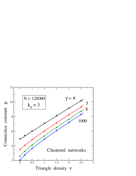
Figure 5: Connective constant $\mu$ vs triangle density $\nu$ for clustered scale-free networks with several values of the exponent $\gamma$: From top to bottom $\gamma$ = 4, 5, 8, and 1000. The networks size is $N$ = 128,000 and the minimum degree $k_{0}=3$. Solid lines correspond to the analytical procedure described in Sec. IV, whereas symbols were derived from enumeration of SAWs in clustered networks. Error bars are less than the symbol size.

V.1 Case $\gamma>3$

In this case the average value $\langle k^{2}\rangle_{N}$ converges to a finite value in the large-size limit, and therefore the connective constant is well defined in this limit. In Fig. 5 we display $\mu$ as a function of the triangle density $\nu$ for clustered scale-free networks with size $N=128,000$, minimum degree $k_{0}=3$, and various values of the exponent $\gamma$. Symbols are data points derived from simulations for $\gamma$ = 4, 5, 8, and 1000. Here the large exponent $\gamma=1000$ is equivalent to the limit $\gamma\to\infty$, as in this case $s_{i}=k_{0}$ for all nodes. Error bars in Fig. 5 are smaller than the symbol size. Lines represent results obtained from the analytical method presented above, and follow closely the data points obtained from the network simulations. For $N=128,000$ the finite-size effect in the connective constant is almost inappreciable for networks with $\gamma>3$.

For $\nu=0$ (no triangles) the connective constant can be directly derived from the mean values $\langle s\rangle_{N}$ and $\langle s^{2}\rangle_{N}$ given in Eqs. (5) and (6), as

$$\mu_{N}=\frac{\langle s^{2}\rangle_{N}}{\langle s\rangle_{N}}-1\;,$$ (29)

as follows from Eq. (19) for unclustered networks. Then, for large $N$, $\mu_{N}$ converges to $\mu_{\infty}$ given in Eq. (21). For clustered networks with $\nu>0$, the connective constant can be obtained by introducing the parameters $z$ and $r$ derived from $\langle s\rangle_{N}$ and $\langle s^{2}\rangle_{N}$ [see Eq. (26)] into the iterative equations (27), or alternatively into the system (28). This gives for different values of $\gamma$ the lines shown in Fig. 5.

For unclustered networks with $\nu>0$, $\mu_{\infty}$ is derived from $\langle k\rangle_{\infty}$ and $\langle k^{2}\rangle_{\infty}$ in Eqs. (2) and (12). For a given network size ($N=128,000$ in Fig. 5), $\mu_{\infty}$ converges to $2\nu$ for large $\nu$, irrespective of the exponent $\gamma$. This comes from the dominant terms in the ratio $\langle k^{2}\rangle_{\infty}/\langle k\rangle_{\infty}$, i.e. $\langle k^{2}\rangle_{\infty}\approx 4\nu^{2}$ and $\langle k\rangle_{\infty}\approx 2\nu$ for $\nu\gg 1$.

The results for the connective constant $\mu_{\infty}$ of unclustered networks are very close to those corresponding to clustered networks, and are not shown in Fig. 5. Both sets of results are in fact indistinguishable within error bars, which are smaller than the symbol size. This is mainly due to the very low probability of high-degree nodes in these networks. This fact, which occurs for $\mu_{\infty}$ in networks with $\gamma>3$, does not happen for networks with $\gamma\leq 3$, where results for $\mu_{N}$ appreciably differ for clustered and unclustered networks (see below).

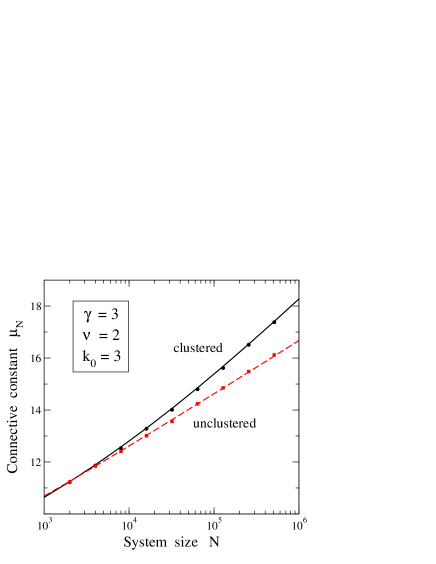
Figure 6: Connective constant $\mu_{N}$ as a function of system size $N$ for scale-free networks with $\gamma=3$ and triangle density $\nu=2$. The solid and dashed lines were obtained analytically for clustered and unclustered (configuration model) networks, respectively. Symbols correspond to results found from simulated scale-free networks. Error bars are smaller than the symbol size.

V.2 Case $\gamma=3$

For scale-free networks with $\gamma=3$ the average value $\langle k^{2}\rangle_{N}$ diverges logarithmically with $N$, see Eq. (8). This behavior controls the asymptotic dependence of the connective constant on system size. In Fig. 6 we present the size-dependent $\mu_{N}$ vs $N$ for scale-free networks with $\gamma=3$ and $\nu=2$. Shown are results for clustered and unclustered (configuration model) networks. As in the case $\gamma>3$ shown above, symbols are data points derived from SAWs in simulated networks, whereas lines were obtained from analytical calculations. For small networks, $\mu_{N}$ is similar for both kinds of networks, and the connective constant corresponding to the clustered ones becomes appreciably larger as the system size increases. For given $N$ and $\nu>0$, we have $\mu_{N}^{\rm cl}>\mu_{N}^{\rm un}$.

For clustered networks (solid line), the procedure to calculate $\mu_{N}$ is the same as that employed above for $\gamma>3$, using the iterative equations (27), and taking into account the adequate expressions for $\langle s\rangle_{N}$ and $\langle s^{2}\rangle_{N}$ given in Eqs. (5) and (7), respectively. We cannot write an exact analytical expression for $\mu_{N}$ as a function of $N$ and $\nu$ for clustered networks, but we can analyze its behavior for large $N$ and $\nu$ from the results of our calculations and network simulations. For large $N$ and relatively small $\nu$, the r.h.s. of the first equation in the iterative system Eq. (27) giving $b_{n}$ is dominated by the contribution of $b_{n-1}$ because $r\gg z$. Then, $b_{n}/b_{n-1}$ converges to $\mu_{N}\approx\langle s^{2}\rangle_{N}/\langle s\rangle_{N}\approx\frac{1}{2}k_{0}\ln N$.

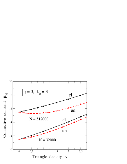
Figure 7: Connective constant $\mu_{N}$ vs triangle density $\nu$ for scale-free networks with $\gamma=3$ and $k_{0}=3$. The data shown correspond to two different network size: $N$ = 512,000 (top) and 32,000 (bottom). Solid and dashed lines correspond to analytical calculations for networks with and without triangles, respectively. Symbols are results derived from network simulations. Error bars are of the order of the symbol size. ‘cl’ and ‘un’ refer to clustered and unclustered SF networks, respectively.

For unclustered networks (dashed line in Fig. 6) $\mu_{N}$ is given by Eq. (22), valid for the configuration model. Here $\langle k\rangle_{N}$ and $\langle k^{2}\rangle_{N}$ are obtained from average values corresponding to $s$-links and $t$-links separately, see Eq. (11). Then, for large $N$ the ratio $\langle k^{2}\rangle_{N}/\langle k\rangle_{N}$ is dominated by the contribution of $s$-links, yielding

$$\mu_{N}\approx\frac{\langle k^{2}\rangle_{N}}{\langle k\rangle_{N}}\approx\frac{\langle s^{2}\rangle_{N}}{\langle s\rangle_{N}+2\nu}\approx\frac{k_{0}^{2}\ln N}{2(k_{0}+\nu)}\;,$$ (30)

which coincides with Eq. (23) for $\nu=0$. This means that for the data shown in Fig. 6 ($\nu=2,k_{0}=3$), the slope of the dashed line for large $N$ is given by $\partial\mu_{N}/\partial\ln N=0.9$. For SF networks with $\gamma=3$ and $\nu=0$, one has $\mu_{N}\sim\frac{1}{2}k_{0}\ln N$ for large $N$, Eq. (23), and we find a slope $\partial\mu/\partial\ln N=1.5$.

In Fig. 7 we show $\mu_{N}$ for networks with $\gamma=3$ as a function of the triangle density $\nu$. We present results for clustered and unclustered networks and two network sizes: $N$ = 32,000 and 512,000 nodes. For both network sizes, $\mu_{N}^{\rm cl}>\mu_{N}^{\rm un}$ for $\nu>0$. For clustered networks with relatively large $N$, $\mu_{N}$ increases monotonically for rising $\nu$, with a slope $d\mu/d\nu$ that grows converging to a value of 2 for large $\nu$. This can be derived from Eq. (37), where the variable $\theta$, defined in (34), is the limit of the ratio $c_{n}/b_{n}$ for large $n$. Taking into account that $c_{n}$ and $b_{n}$ are the mean number of SAWs ending in $t$-links and $s$-links, respectively, one expects that $\theta$ increases as the triangle density (or the number of $t$-links) increases. Thus, we have $\theta\lesssim\langle t\rangle/\langle s\rangle$, as can be found from numerical solutions of Eq. (28) or Eq. (37). Then, for large $\nu$, i.e. $\alpha\gg 1$, we have $\theta\gg 1$, $\mu_{N}\gg 1$, $\sigma=1/\mu_{N}\ll 1$, and from Eq. (28) we find that $\theta\to 2\nu/z$. Using again Eq. (28), one has $\mu_{N}=r+z\theta-1$, with $r$ and $z$ independent of $\nu$, so that $\partial\mu_{N}/\partial\nu=z\,\partial\theta/\partial\nu$, which converges to 2 for large $\nu$.

For unclustered networks (configuration model) we have for large $\nu$, see Eq. (22):

$$\mu_{N}=\frac{\langle k^{2}\rangle_{N}}{\langle k\rangle_{N}}-1\approx\frac{k_{0}^{2}\ln N}{2\nu}+2\nu\;,$$ (31)

and for a given $N$, $\partial\mu_{N}/\partial\nu\to 2$ for large $\nu$. However, for large $N$ this convergence is slower than in the case of clustered networks, as can be observed in Fig. 7.

Summarizing the results presented in this section for clustered networks with $\gamma=3$, we find that for large $N$ or $\nu$, the leading contribution to the connective constant $\mu_{N}$ appears to be either a function $f(N)$ or another function $g(\nu)$, depending on the values of both variables $N$ and $\nu$. This means that the behavior of $\mu_{N}$ can be described as $\mu_{N}\sim f(N)+g(\nu)+h(N,\nu)$, where we include a contribution $h(N,\nu)$ that becomes negligible for large $N$ or $\nu$. For $\gamma=3$ we have $f(N)\to\frac{1}{2}k_{0}\ln N$ for large $N$ and $g(\nu)\to 2\nu$ for large $\nu$. Then, for $k_{0}\ln N\gg\nu$, one has $\mu_{N}\approx\frac{1}{2}k_{0}\ln N$, whereas for $k_{0}\ln N\ll\nu$, $\mu_{N}\approx 2\nu$. This indicates that one has a crossover from a parameter region where the behavior of the connective constant is dominated by the scale-free character of the degree distribution $P_{\rm sf}(s)$, to another region where it is controlled by the cluster distribution (triangles). This is not a sharp crossover, and in the intermediate region a simple decomposition of $\mu_{N}$ into two independent contributions is not valid, as indicated above with the function $h(N,\nu)$. For a given $N$, the crossover occurs for a triangle density $\nu_{c}\sim\frac{1}{4}k_{0}\ln N$. Thus, for $N=5\times 10^{5}$, $\nu_{c}\approx 10$, and for $N=10^{4}$, $\nu_{c}\approx 7$.

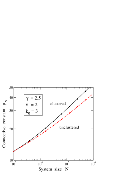
Figure 8: Connective constant $\mu_{N}$ as a function of system size $N$ for scale-free networks with $\gamma=2.5$ and triangle density $\nu=2$. The solid and dashed lines were obtained analytically for clustered and unclustered networks, respectively. Symbols correspond to results obtained from simulated scale-free networks. Error bars are less than the symbol size.

V.3 Case $\gamma<3$

In this case the average value $\langle k^{2}\rangle_{N}$ scales as a power of the network size $N$, similar to $\langle s^{2}\rangle_{N}$ in Eq. (10), and this dependence controls the behavior of the connective constant $\mu_{N}$. In Fig. 8 we display $\mu_{N}$ as a function of $N$ for clustered and unclustered SF networks with exponent $\gamma=2.5$ and triangle density $\nu=2$. As in previous figures, symbols are data points obtained from enumeration of SAWs in simulated networks, and lines correspond to calculations following the procedure described in Sec. IV and Appendix A. As for $\gamma=3$ (see above), the connective constant for $\gamma=2.5$ is similar for clustered and unclustered networks for relatively small $N$. The results for both kinds of networks differ progressively as $N$ increases, being larger the value for clustered networks, as in Fig. 6 for $\gamma=3$. Note, however, that the vertical scale in Fig. 8 is logarithmic in contrast to Fig. 6, where it is linear.

For clustered networks with relatively large $N$ one has $\mu_{N}\approx\langle s^{2}\rangle_{N}/\langle s\rangle_{N}$, as reasoned above for $\gamma=3$. We find for $\gamma=2.5$ a dependence $\mu_{N}\approx\sqrt{k_{0}}N^{1/4}$. This agrees with the results shown in Fig. 8 (solid line), where the derivative $\partial\ln\mu_{N}/\partial\ln N$ converges to 0.25 for $N\to\infty$. In fact this derivative rises for increasing $N$, and for $N=10^{6}$ it is already very close to its asymptotic limit.

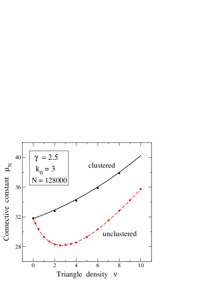
Figure 9: Connective constant $\mu_{N}$ vs triangle density $\nu$ for clustered SF networks with $\gamma=2.5$: the solid line is the result of the analytical model described in Sec. IV, whereas solid circles are data points derived from enumeration of SAWs in simulated clustered networks. The dashed line and solid squares correspond to unclustered networks (configuration model). Error bars are less than the symbol size.

For unclustered networks with $\gamma=2.5$ we have

$$\mu_{N}\approx\frac{\langle k^{2}\rangle_{N}}{\langle k\rangle_{N}}\approx\frac{3k_{0}^{3/2}}{3k_{0}+2\nu}N^{1/4}\;,$$ (32)

which coincides with Eq. (24) for $\nu=0$. Thus, for large $N$ the connective constant behaves in a similar way to clustered networks, i.e. $\mu_{N}\approx AN^{1/4}$, but now the prefactor in Eq. (32) depends on the triangle density $\nu$. For the case presented in Fig. 8 ($\nu=2$) we find $A=1.20$ (large-$N$ limit of dashed line), in agreement with the results obtained from simulations of unclustered networks (solid squares). We note that the convergence to the power-law behavior $\mu_{N}\sim N^{1/4}$ is faster (occurs for smaller size $N$) for clustered than for unclustered networks. In general, for $\gamma<3$ one has $\mu_{N}\sim N^{(3-\gamma)/2}$, as can be derived from the expressions for the mean values $\langle s\rangle$ and $\langle s^{2}\rangle$ given in Sec. II.B.

In Fig. 9 we show the dependence of $\mu_{N}$ on triangle density $\nu$ for clustered and unclustered (configuration model) networks with $\gamma=2.5$ and system size $N=128,000$ nodes. The connective constant for clustered networks increases monotonically with the parameter $\nu$ and the slope $\partial\mu_{N}/\partial\nu$ grows and converges to 2 for large $\nu$. This happens in a way similar to the case $\gamma=3$ discussed above (Fig. 7).

For unclustered networks (solid squares and dashed line in Fig. 9) it is remarkable the decrease in $\mu_{N}$ for increasing $\nu$ close to $\nu=0$ for $N$ = 128,000, i.e., for small $\nu$ we have $\partial\mu_{N}/\partial\nu<0$. This is due to the fact that, for growing $\nu$, the relative increase is larger for $\langle k\rangle_{N}$ than for $\langle k^{2}\rangle_{N}$, so the ratio $\langle k^{2}\rangle_{N}/\langle k\rangle_{N}$ decreases for small $\nu$. This becomes more appreciable for larger network size. In the $\mu_{N}$ vs $\nu$ curve shown in Fig. 9 one has a minimum of $\mu_{N}$ for $\nu=2.7$. For higher triangle density $\nu$, the slope of the curve increases, approaching the line corresponding to clustered networks. For a given system size $N$, the quotient $\langle k^{2}\rangle_{N}/\langle k\rangle_{N}$ yielding $\mu_{N}$ is dominated for large $\nu$ by the term $\langle t^{2}\rangle=4\nu(\nu+1)$ in the numerator [see Eqs. (11) and (12)], and $\langle t\rangle=2\nu$ in the denominator, so $\partial\mu_{N}/\partial\nu\to 2$ in the large-$\nu$ limit.

Summarizing the results shown in this section for clustered networks with $\gamma=2.5$, we obtain that for large $N$ or $\nu$, the connective constant behaves as $\mu_{N}\sim\sqrt{k_{0}}N^{1/4}+g(\nu)+h(N,\nu)$, with $g(\nu)\sim 2\nu$ for large $\nu$. As in the case $\gamma=3$ discussed above, one has in general a contribution $h(N,\nu)$ that becomes negligible in the limits discussed here, and for which we do not have an analytical expression. Then, for $N\gg\nu^{4}$ we have $\mu_{N}\approx\sqrt{k_{0}}N^{1/4}$, and for $N\ll\nu^{4}$, $\mu_{N}\approx 2\nu$. For a given $N$, there appears a crossover at a triangle density $\nu_{c}\sim\frac{1}{2}\sqrt{k_{0}}N^{1/4}$. On one side, for $\nu<\nu_{c}$, the behavior of the connective constant $\mu_{N}$ is dominated by a power of $N$, corresponding to the scale-free degree distribution of single links $P_{\rm sf}(s)$. On the other side, for $\nu>\nu_{c}$ , $\mu_{N}$ is controlled by the distribution of triangles $Q(t)$. For $\gamma=2.5$ and $N=5\times 10^{5}$ we have $\nu_{c}\approx 23$, and for $N=10^{4}$, $\nu_{c}\approx 9$. In general, for $\gamma<3$ the crossover takes place at a triangle density $\nu_{c}$ given by

$$\nu_{c}\sim\frac{1}{2}\,\frac{\gamma-2}{3-\gamma}\,k_{0}^{\gamma-2}\,N^{(3-\gamma)/2}\;.$$ (33)

Note that in this expression the exponent $(3-\gamma)/2$ is the same as that of the connective constant for large $N$: $\mu_{N}\sim N^{(3-\gamma)/2}$. In the parameter region where the behavior of $\mu_{N}$ is controlled by the large-degree tail of the power law $P_{\rm sf}(s)$ (i.e., $\nu<\nu_{c}$), the connective constant can be described by an expression $\mu_{N}\sim N^{\beta}$, where $\beta$ is a variable parameter that evolves from zero for small system size to $(3-\gamma)/2$ for large $N$. Specifically, one can define $\beta$ as the logarithmic derivative $\beta=d\ln\mu_{N}/d\ln N$. Thus, from the results shown in Fig. 8 for clustered networks with $\gamma=2.5$ we find a parameter $\beta$ in the interval from 0.14 for $N=10^{3}$ to 0.247 for $N=7\times 10^{6}$. The latter value is close to the exponent $(3-\gamma)/2=0.25$ corresponding to a pure scale-free network. The variable parameter $\beta$ is in principle regulated by the function $h(N,\nu)$ mentioned above, but we do not know a precise expression for it.

VI Conclusions

Self-avoiding walks are a suitable means to analyze the long-distance properties of complex networks. We have studied the connective constant for clustered scale-free networks by using an iterative analytical procedure that converges in a few steps. The results of these calculations agree well with those derived from direct enumeration of SAWs in simulated networks. These data have been compared with those corresponding to unclustered networks with the same degree distribution $P(k)$. For large unclustered networks, the number of SAWs rises with the number of steps $n$ as $a_{n}/a_{n-1}\approx\langle k^{2}\rangle/\langle k\rangle-1$, but in the presence of clusters the ratio $a_{n}/a_{n-1}$ depends explicitly on the distribution of both $s$ and $t$-links.

Our results can be classified into two different groups, depending on the exponent $\gamma$ of the power-law degree distribution in this kind of networks. Comparing clustered and unclustered networks, the conclusions obtained for $\gamma>3$ differ from those found for $\gamma\leq 3$. For networks with $\gamma>3$, one has a well-defined connective constant $\mu_{\infty}$ in the thermodynamic limit ($N\to\infty$). Adding motifs (here triangles) to the networks causes an increase in $\mu$, mainly due to a rise in the average value $\langle k^{2}\rangle$. Nevertheless, we find a small numerical difference in $\mu$ for clustered and unclustered networks with the same degree distribution $P(k)$.

For $\gamma\leq 3$, the size-dependent connective constant $\mu_{N}$ is similar for clustered and unclustered networks with the same $P(k)$ when one considers small network sizes ($N\lesssim 10^{3}$). This behavior changes for larger networks, where $\mu_{N}^{\rm cl}>\mu_{N}^{\rm un}$. This difference is more apparent for decreasing $\gamma$, due to the larger number of high-degree nodes. For SF networks with $\gamma\leq 3$, $\mu_{N}$ increases with system size $N$, and diverges for $N\to\infty$. Depending on the values of the system size $N$ and triangle density $\nu$, we find two regimes for the connective constant $\mu_{N}$. For a given $N$ there appears a crossover from a region where $\mu_{N}$ is controlled by the scale-free degree distribution $P_{\rm sf}(s)$ of single links (for small $\nu$) to another parameter region where the behavior of $\mu_{N}$ is dominated by the triangle distribution $Q(t)$ (large $\nu$). The crossover between both regimes appears at a triangle density $\nu_{c}$ such that $\nu_{c}\sim\frac{1}{4}k_{0}\ln N$ for $\gamma=3$ and $\nu_{c}\sim N^{(3-\gamma)/2}$ for $\gamma<3$ [see Eq. (33)].

The numerical results for clustered and unclustered scale-free networks may change when different degree cutoffs are employed. This is particularly relevant for $\gamma<3$, since the dependence of $\mu_{N}$ on system size is important. In this respect, to avoid undesired correlations between degrees of adjacent nodes, we have employed here a degree cutoff $k_{\rm cut}=N^{1/2}$.

Other probability distributions, different from the short-tailed Poisson type considered here for triangles, may be introduced to change more strongly the long-degree tail in the overall degree distribution $P(k)$. Thus, a power-law distribution for the triangles can cause a competition between the exponents of both distributions (for $s$-links and $t$-links), which can change the asymptotic behavior of SAWs in such networks in comparison to those presented here.

There are clear similarities between the asymptotic behavior of the connective constant ($\mu_{\infty}$ or $\mu_{N}$) derived from SAWs and the ferromagnetic-paramagnetic transition temperature for the Ising model in this kind of networks Herrero (2015). This is related to the fact that both directly depend on the mean value $\langle k^{2}\rangle$, which changes with the exponent $\gamma$ of the degree distribution. The extent of such similarities in the case of clustered networks is an open question that should be further investigated.

Appendix A Calculation of the connective constant

In this section we present a derivation of the connective constant in clustered networks as the asymptotic limit of the ratio $a_{n}/a_{n-1}$. It is based on the coupled iterative equations given in Eq. (27). To find the values of $b_{n}$ and $c_{n}$ for large $n$, we define

$$\theta_{n}=\frac{c_{n}}{b_{n}};\hskip 56.9055pt\theta=\lim_{n\to\infty}\theta_{n}$$ (34)

and

$$\sigma_{n}=\frac{b_{n}}{b_{n+1}};\hskip 56.9055pt\sigma=\lim_{n\to\infty}\sigma_{n}$$ (35)

Then, from Eqs. (27), (34), and (35), we have

$$\theta_{n}=\frac{\alpha+\theta_{n-1}(\alpha+1)-\sigma_{n-3}\sigma_{n-2}\alpha-\theta_{n-3}\sigma_{n-3}\sigma_{n-2}\alpha}{r-1+\theta_{n-1}z}\;,$$ (36)

and taking the limit $n\to\infty$:

$$\theta=\frac{\alpha+\theta(\alpha+1)-\sigma^{2}\alpha(1+\theta)}{r-1+\theta z}\;.$$ (37)

Moreover, from Eq. (27) we have

$$\frac{b_{n+1}}{b_{n}}=r-1+\theta_{n}z\;,$$ (38)

so that

$$\frac{1}{\sigma}=\lim_{n\to\infty}\frac{b_{n+1}}{b_{n}}=r-1+\theta z\;.$$ (39)

Eqs. (37) and (39) can be used to obtain the limits $\theta$ and $\sigma$, as well as to find the simplified expression

$$\frac{\theta}{\sigma}=\alpha+\theta(\alpha+1)-\sigma^{2}\alpha(1+\theta)\;.$$ (40)

Combining Eqs. (39) and (40), one can eliminate $\sigma$, which yields a quartic equation in $\theta$.

The connective constant $\mu$ is defined as

$$\mu=\lim_{n\to\infty}\frac{a_{n+1}}{a_{n}}\;.$$ (41)

Taking into account that $a_{n}=b_{n}+c_{n}$ [Eq. (25)], we have

$$\mu=\lim_{n\to\infty}\frac{1+\theta_{n+1}}{\sigma_{n}+\theta_{n}\sigma_{n}}=\frac{1}{\sigma}\;.$$ (42)

Using Eq. (42) we can rewrite Eq. (40) as

$$\theta\mu^{3}-(\theta\alpha+\theta+\alpha)\mu^{2}+\alpha(1+\theta)=0\;,$$ (43)

which can be used, along with Eq. (39), to form the system of Eq. (28) in the text.

We note that the asymptotic limit of both $b_{n+1}/b_{n}$ and $c_{n+1}/c_{n}$ is also $\mu$. In fact, from Eqs. (35) and (42), we have

$$\lim_{n\to\infty}\frac{b_{n+1}}{b_{n}}=\frac{1}{\sigma}=\mu\;,$$ (44)

and

$$\lim_{n\to\infty}\frac{c_{n+1}}{c_{n}}=\lim_{n\to\infty}\frac{c_{n+1}}{b_{n+1}}\frac{b_{n+1}}{b_{n}}\frac{b_{n}}{c_{n}}=\theta\mu\frac{1}{\theta}=\mu$$ (45)

For $\gamma\leq 3$, we have defined in Sec III a size-dependent connective constant $\mu_{N}$ . In this case, the limits to infinity presented in this Appendix have no sense. However, the ratios $a_{n}/a_{n-1}$, $b_{n}/b_{n-1}$, and $c_{n}/c_{n-1}$ considered here converge with our present method for relatively low number of steps, $n\ll N$, as indicated in Sec. IV (see Fig. 4).

References

- Dorogovtsev and Mendes (2003) S. N. Dorogovtsev and J. F. F. Mendes, Evolution of Networks: From Biological Nets to the Internet and WWW (Oxford University, Oxford, 2003).
- Cohen and Havlin (2010) R. Cohen and S. Havlin, Complex networks. Structure, robustness and function (Cambridge University Press, Cambridge, 2010).
- Albert and Barabási (2002) R. Albert and A. L. Barabási, Rev. Mod. Phys. 74, 47 (2002).
- Strogatz (2001) S. H. Strogatz, Nature 410, 268 (2001).
- von Ferber and Holovatch (2013) C. von Ferber and Y. Holovatch, Eur. Phys. J. Spec. Topics 216, 49 (2013).
- da F. Costa et al. (2007) L. da F. Costa, F. A. Rodrigues, G. Travieso, and P. R. Villas Boas, Adv. Phys. 56, 167 (2007).
- Newman (2010) M. E. J. Newman, Networks. An Introduction (Oxford University Press, New York, 2010).
- Moore and Newman (2000) C. Moore and M. E. J. Newman, Phys. Rev. E 61, 5678 (2000).
- Kuperman and Abramson (2001) M. Kuperman and G. Abramson, Phys. Rev. Lett. 86, 2909 (2001).
- Hebert-Dufresne et al. (2010) L. Hebert-Dufresne, P.-A. Noel, V. Marceau, A. Allard, and L. J. Dube, Phys. Rev. E 82, 036115 (2010).
- Bauer and Lizier (2012) F. Bauer and J. T. Lizier, EPL 99, 68007 (2012).
- Liu et al. (2017) Q.-H. Liu, W. Wang, M. Tang, T. Zhou, and Y.-C. Lai, Phys. Rev. E 95, 042320 (2017).
- Watts and Strogatz (1998) D. J. Watts and S. H. Strogatz, Nature 393, 440 (1998).
- Herrero (2002) C. P. Herrero, Phys. Rev. E 66, 046126 (2002).
- Pandit and Amritkar (2001) S. A. Pandit and R. E. Amritkar, Phys. Rev. E 63, 041104 (2001).
- Moreno et al. (2004) Y. Moreno, M. Nekovee, and A. F. Pacheco, Phys. Rev. E 69, 066130 (2004).
- Candia (2007) J. Candia, Phys. Rev. E 75, 026110 (2007).
- Jasch and Blumen (2001) F. Jasch and A. Blumen, Phys. Rev. E 64, 066104 (2001).
- Almaas et al. (2003) E. Almaas, R. V. Kulkarni, and D. Stroud, Phys. Rev. E 68, 056105 (2003).
- Newman (2003) M. E. J. Newman, SIAM Rev. 45, 167 (2003).
- Noh and Rieger (2004) J. D. Noh and H. Rieger, Phys. Rev. Lett. 92, 118701 (2004).
- Costa and Travieso (2007) L. d. F. Costa and G. Travieso, Phys. Rev. E 75, 016102 (2007).
- Lopez Millan et al. (2012) V. M. Lopez Millan, V. Cholvi, L. Lopez, and A. Fernandez Anta, Networks 60, 71 (2012).
- Siganos et al. (2003) G. Siganos, M. Faloutsos, P. Faloutsos, and C. Faloutsos, IEEE ACM Trans. Netw. 11, 514 (2003).
- Albert et al. (1999) R. Albert, H. Jeong, and A. L. Barabási, Nature 401, 130 (1999).
- Newman (2001) M. E. J. Newman, Proc. Natl. Acad. Sci. USA 98, 404 (2001).
- Jeong et al. (2001) H. Jeong, S. P. Mason, A. L. Barabási, and Z. N. Oltvai, Nature 411, 41 (2001).
- Goh et al. (2002) K. I. Goh, E. S. Oh, H. Jeong, B. Kahng, and D. Kim, Proc. Natl. Acad. Sci. USA 99, 12583 (2002).
- Goh et al. (2003) K. I. Goh, D. S. Lee, B. Kahng, and D. Kim, Phys. Rev. Lett. 91, 148701 (2003).
- Radicchi and Fortunato (2009) F. Radicchi and S. Fortunato, Phys. Rev. Lett. 103, 168701 (2009).
- Dorogovtsev et al. (2002) S. N. Dorogovtsev, A. V. Goltsev, and J. F. F. Mendes, Phys. Rev. E 66, 016104 (2002).
- Herrero (2004) C. P. Herrero, Phys. Rev. E 69, 067109 (2004).
- Bartolozzi et al. (2006) M. Bartolozzi, T. Surungan, D. B. Leinweber, and A. G. Williams, Phys. Rev. B 73, 224419 (2006).
- Dorogovtsev et al. (2008) S. N. Dorogovtsev, A. V. Goltsev, and J. F. F. Mendes, Rev. Mod. Phys. 80, 1275 (2008).
- Herrero (2009) C. P. Herrero, Eur. Phys. J. B 70, 435 (2009).
- Dommers et al. (2010) S. Dommers, C. Giardina, and R. van der Hofstad, J. Stat. Phys. 141, 638 (2010).
- Ostilli et al. (2011) M. Ostilli, A. L. Ferreira, and J. F. F. Mendes, Phys. Rev. E 83, 061149 (2011).
- Kim et al. (2016) Y. Kim, S. Park, and S.-H. Yook, Phys. Rev. E 94, 042309 (2016).
- Tishby et al. (2016) I. Tishby, O. Biham, and E. Katzav, J. Phys. A: Math. Theor. 49, 285002 (2016).
- Adamic et al. (2001) L. A. Adamic, R. M. Lukose, A. R. Puniyani, and B. A. Huberman, Phys. Rev. E 64, 046135 (2001).
- de Gennes (1979) P. G. de Gennes, Scaling Concepts in Polymer Physics (Cornell University, Ithaca, NY, 1979).
- Orlandini and Whittington (2007) E. Orlandini and S. G. Whittington, Rev. Mod. Phys. 79, 611 (2007).
- Beaton et al. (2012) N. R. Beaton, A. J. Guttmann, and I. Jensen, J. Phys. A: Math. Theor. 45, 055208 (2012).
- Guttmann et al. (2014) A. J. Guttmann, I. Jensen, and S. G. Whittington, J. Phys. A: Math. Theor. 47, 015004 (2014).
- Maier and Radler (1999) B. Maier and J. O. Radler, Phys. Rev. Lett. 82, 1911 (1999).
- Witz et al. (2008) G. Witz, K. Rechendorff, J. Adamcik, and G. Dietler, Phys. Rev. Lett. 101, 148103 (2008).
- Herrero (1995) C. P. Herrero, J. Phys.: Condens. Matter 7, 8897 (1995).
- Herrero (2014) C. P. Herrero, Chem. Phys. 439, 49 (2014).
- Kremer et al. (1982) K. Kremer, A. Baumgärtner, and K. Binder, J. Phys. A: Math. Gen. 15, 2879 (1982).
- Clisby (2010) N. Clisby, Phys. Rev. Lett. 104, 055702 (2010).
- Guttmann and Jacobsen (2013) A. J. Guttmann and J. L. Jacobsen, J. Phys. A: Math. Theor. 46, 435004 (2013).
- Herrero and Saboyá (2003) C. P. Herrero and M. Saboyá, Phys. Rev. E 68, 026106 (2003).
- Herrero (2005a) C. P. Herrero, Phys. Rev. E 71, 016103 (2005a).
- Hotta (2014) Y. Hotta, Phys. Rev. E 90, 052821 (2014).
- Fricke and Janke (2014) N. Fricke and W. Janke, Phys. Rev. Lett. 113, 255701 (2014).
- Rapaport (1985) D. C. Rapaport, J. Phys. A 18, 113 (1985).
- Privman et al. (1991) V. Privman, P. C. Hohenberg, and A. Aharony, in Phase Transitions and Critical Phenomena, edited by C. Domb and J. L. Lebowitz (Academic Press, London, 1991), vol. 14.
- Herrero (2005b) C. P. Herrero, J. Phys. A: Math. Gen. 38, 4349 (2005b).
- Herrero (2007) C. P. Herrero, Eur. Phys. J. B 56, 71 (2007).
- Holme and Kim (2002) P. Holme and B. J. Kim, Phys. Rev. E 65, 026107 (2002).
- Klemm and Eguiluz (2002) K. Klemm and V. M. Eguiluz, Phys. Rev. E 65, 036123 (2002).
- Serrano and Boguñá (2005) M. A. Serrano and M. Boguñá, Phys. Rev. E 72, 036133 (2005).
- Klaise and Johnson (2018) J. Klaise and S. Johnson, Phys. Rev. E 97, 012302 (2018).
- Lopez et al. (2018) F. A. Lopez, P. Barucca, M. Fekom, and A. C. C. Coolen, J. Phys. A: Math. Theor. 51, 085101 (2018).
- Newman (2009) M. E. J. Newman, Phys. Rev. Lett. 103, 058701 (2009).
- Miller (2009) J. C. Miller, Phys. Rev. E 80, 020901 (2009).
- Heath and Parikh (2011) L. S. Heath and N. Parikh, Physica A 390, 4577 (2011).
- Herrero (2015) C. P. Herrero, Phys. Rev. E 91, 052812 (2015).
- Huang et al. (2013) X. Huang, S. Shao, H. Wang, S. V. Buldyrev, H. E. Stanley, and S. Havlin, EPL 101, 18002 (2013).
- Gleeson (2009) J. P. Gleeson, Phys. Rev. E 80, 036107 (2009).
- Gleeson et al. (2010) J. P. Gleeson, S. Melnik, and A. Hackett, Phys. Rev. E 81, 066114 (2010).
- Radicchi and Castellano (2016) F. Radicchi and C. Castellano, Phys. Rev. E 93, 030302 (2016).
- Molina and Stone (2012) C. Molina and L. Stone, J. Theor. Biol. 315, 110 (2012).
- Wang et al. (2012) B. Wang, L. Cao, H. Suzuki, and K. Aihara, J. Theor. Biol. 304, 121 (2012).
- Newman (2005) M. E. J. Newman, Contemp. Phys. 46, 323 (2005).
- Catanzaro et al. (2005) M. Catanzaro, M. Boguñá, and R. Pastor-Satorras, Phys. Rev. E 71, 027103 (2005).
- Iglói and Turban (2002) F. Iglói and L. Turban, Phys. Rev. E 66, 036140 (2002).
- Yoon et al. (2011) S. Yoon, A. V. Goltsev, S. N. Dorogovtsev, and J. F. F. Mendes, Phys. Rev. E 84, 041144 (2011).
- Sokal (1995) A. D. Sokal, in Monte Carlo and Molecular Dynamics Simulations in Polymer Science, edited by K. Binder (Oxford University, Oxford, 1995), pp. 47–124.
- Bollobás (1998) B. Bollobás, Modern Graph Theory (Springer-Verlag, New York, 1998).
- Dorogovtsev and Mendes (2002) S. N. Dorogovtsev and J. F. F. Mendes, Adv. Phys. 51, 1079 (2002).