Entanglement detection with scrambled data

Abstract

In the usual entanglement detection scenario the possible measurements and the corresponding data are assumed to be fully characterized. We consider the situation where the measurements are known, but the data is scrambled, meaning the assignment of the probabilities to the measurement outcomes is unknown. We investigate in detail the two-qubit scenario with local measurements in two mutually unbiased bases. First, we discuss the use of entropies to detect entanglement from scrambled data, showing that Tsallis- and Rényi entropies can detect entanglement in our scenario, while the Shannon entropy cannot. Then, we introduce and discuss scrambling-invariant families of entanglement witnesses. Finally, we show that the set of non-detectable states in our scenario is non-convex and therefore in general hard to characterize.

I Introduction

The characterization of entanglement is a central problem in many experiments. From a theoretical point of view, methods like quantum state tomography or entanglement witnesses are available. In practice, however, the situation is not so simple, as experimental procedures are always imperfect, and the imperfections are difficult to characterize. To give an example, the usual schemes for quantum tomography require the performance of measurements in a well-characterized basis such as the Pauli basis, but in practice the measurements may be misaligned in an uncontrolled manner. Thus, the question arises how to characterize states with relaxed assumptions on the measurements or on the obtained data.

For the case that the measurements are not completely characterized, several methods exist to learn properties of quantum states in a calibration-robust or even device-independent manner seevinck ; squashing ; gittsovich ; bancal ; bancalexp . But even if the measurements are well characterized and trustworthy, there may be problems with the interpretation of the observed probabilities. For instance, in some ion trap experiments rowe2001experimental the individual ions cannot be resolved, so that some of the observed frequencies cannot be uniquely assigned to the measurement operators in a quantum mechanical description. More generally, one can consider the situation where the connection between the outcomes of a measurement and the observed frequencies is lost, in the sense that the frequencies are permuted in an uncontrolled way. We call this situation the “scrambled data” scenario. Still it can be assumed that the measurements have a well-characterized quantum mechanical description; so the considered situation is complementary to the calibration-robust or device-independent scenario.

In this paper, we present a detailed study of different methods of entanglement detection using scrambled data. After explaining the setup and the main definitions, our focus lies on the two-qubit case and Pauli measurements. We first study the use of entropies for entanglement detection. Entropies are natural candidates for this task, as they are invariant under permutations of the probabilities. We demonstrate that Tsallis- and Rényi entropies can detect entanglement in our scenario, while the Shannon entropy is sometimes useless. For deriving our criteria, we prove some entropic uncertainty relations, which may be of independent interest.

Second, we introduce scrambling invariant entanglement witnesses. The key observation is here that for certain witnesses the permutation of the data corresponds to the evaluation of another witness, so that the scrambling of the data does not matter.

Third, we characterize the states for which the scrambled data may origin from a separable state, meaning that their entanglement cannot be detected in the scrambled data scenario. We show that this set of states is generally not convex, which gives an intuition why entanglement detection with scrambled data is a hard problem in general.

II Setup and Definitions

Consider an experiment with two qubits and local dichotomic measurements $A\otimes B$, the data then consists of four outcome probabilities $p(A=\pm 1,B=\pm 1)$. We define the scrambled data as a random permutation of these probabilities within but not in-between measurements, such that the assignment of probabilities to outcomes is forgotten. The restriction that permutations in-between measurements are excluded is natural since they are generically inconsistent because the probabilities within a measurement do not sum up to one anymore.

We denote the Pauli matrices by $\sigma_{x}$, $\sigma_{y}$, and $\sigma_{z}$ and the corresponding eigenvectors as $\ket{\pm}$, $\ket{\text{y}^{\pm}}$, and $\ket{0},\ket{1}$, respectively. As an example for scrambled data, we consider the singlet state $\ket{\psi^{-}}=(\ket{+-}-\ket{-+})/\sqrt{2}$ and the product state $\ket{0}\otimes\ket{+}$. In order to detect the entanglement of $\ket{\psi^{-}}$, it makes sense to perform the local measurements $\sigma_{x}\otimes\sigma_{x}$ and $\sigma_{z}\otimes\sigma_{z}$, as there exists an entanglement witness $W=\mathds{1}+\sigma_{x}\otimes\sigma_{x}+\sigma_{z}\otimes\sigma_{z}$ detecting this state guhne2009entanglement . These measurements yield the outcome probabilities $p_{++}$, $p_{+-}$, $p_{-+}$, and $p_{--}$ and $p_{00}$, $p_{01}$, $p_{10}$, and $p_{11}$, respectively.

	$\ket{\psi^{-}}=(\ket{+-}-\ket{-+})/\sqrt{2}$				$\ket{+}\otimes\ket{0}$
	$p_{++}$	$p_{+-}$	$p_{-+}$	$p_{--}$	$p_{++}$	$p_{+-}$	$p_{-+}$	$p_{--}$
$\sigma_{x}\otimes\sigma_{x}$	$0$	$\frac{1}{2}$	$\frac{1}{2}$	$0$	$\frac{1}{2}$	$\frac{1}{2}$	$0$	$0$
$\sigma_{z}\otimes\sigma_{z}$	$0$	$\frac{1}{2}$	$\frac{1}{2}$	$0$	$\frac{1}{2}$	$0$	$\frac{1}{2}$	$0$

Table 1: This table shows the measurement data for the singlet state and the product state $\ket{+}\otimes\ket{0}$ and local measurements $\sigma_{x}\otimes\sigma_{x}$ and $\sigma_{z}\otimes\sigma_{z}$. The scrambled data is the same for the two states. Thus, detecting the entanglement of the singlet state with these measurements is impossible using only the scrambled data.

From Table 1, we clearly see that the measurement data is different for the two states. However, it is easy to see that there is no way of distinguishing the two states using these measurements if one has access only to the scrambled data since the probability distributions are mere permutations of each other. Thus, it is impossible to detect the entanglement of the singlet state because there is a separable state realizing the same scrambled data. We call states whose scrambled data can be realized by a separable state possibly separable as the entanglement cannot be detected in this scenario.

The above observation motivates to focus specifically on the local measurements $\sigma_{x}\otimes\sigma_{x}$ and $\sigma_{z}\otimes\sigma_{z}$ in the following analysis. However, all results hold more generally for local measurements $A_{1}\otimes B_{1}$ and $A_{2}\otimes B_{2}$ if the eigenstates of both $A_{1},A_{2}$ and $B_{1},B_{2}$ form mutually unbiased bases. This is clear from the Bloch sphere representation because any orthogonal basis can be rotated to match the analysis in this work. Indeed, in dimension two and three, all pairs of mutually unbiased bases are equivalent under local unitaries brierley2009all , including the locally two-dimensional case considered here.

III Entropic uncertainty relations

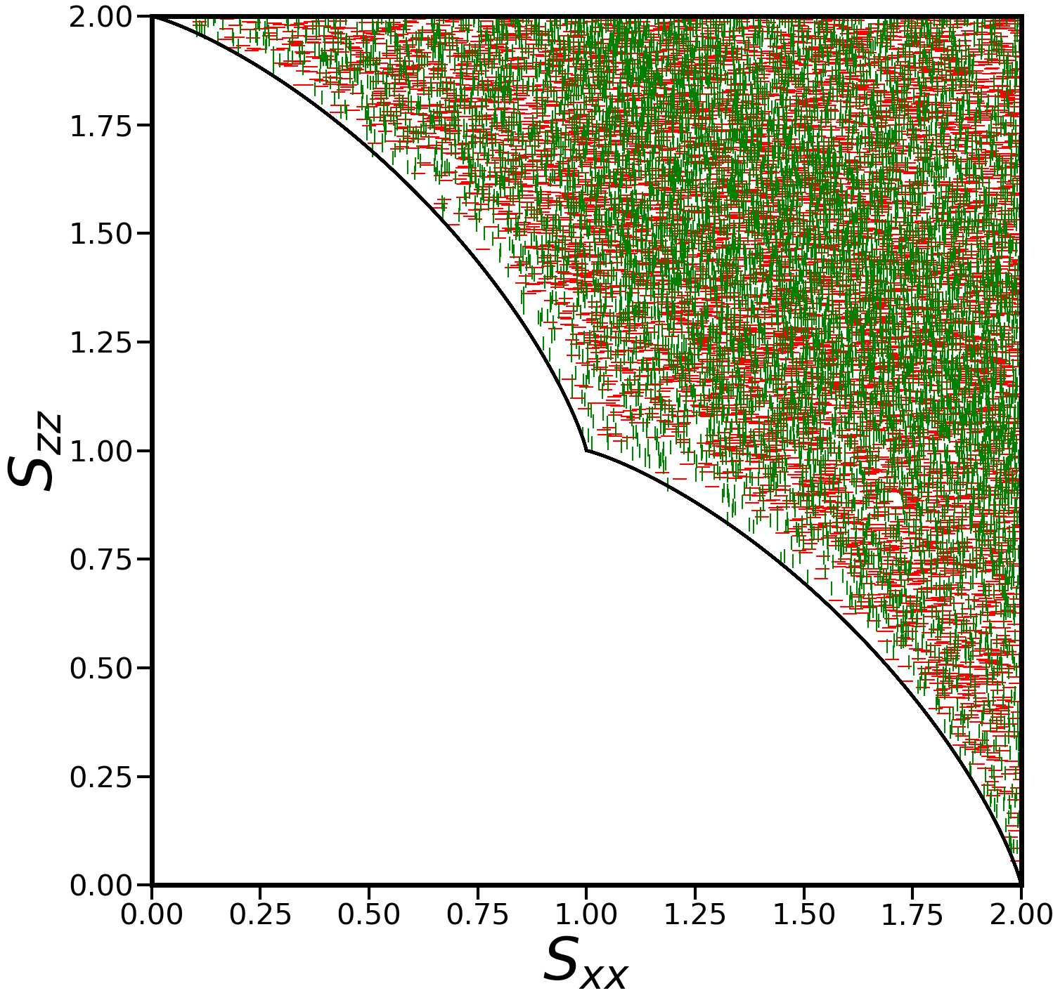
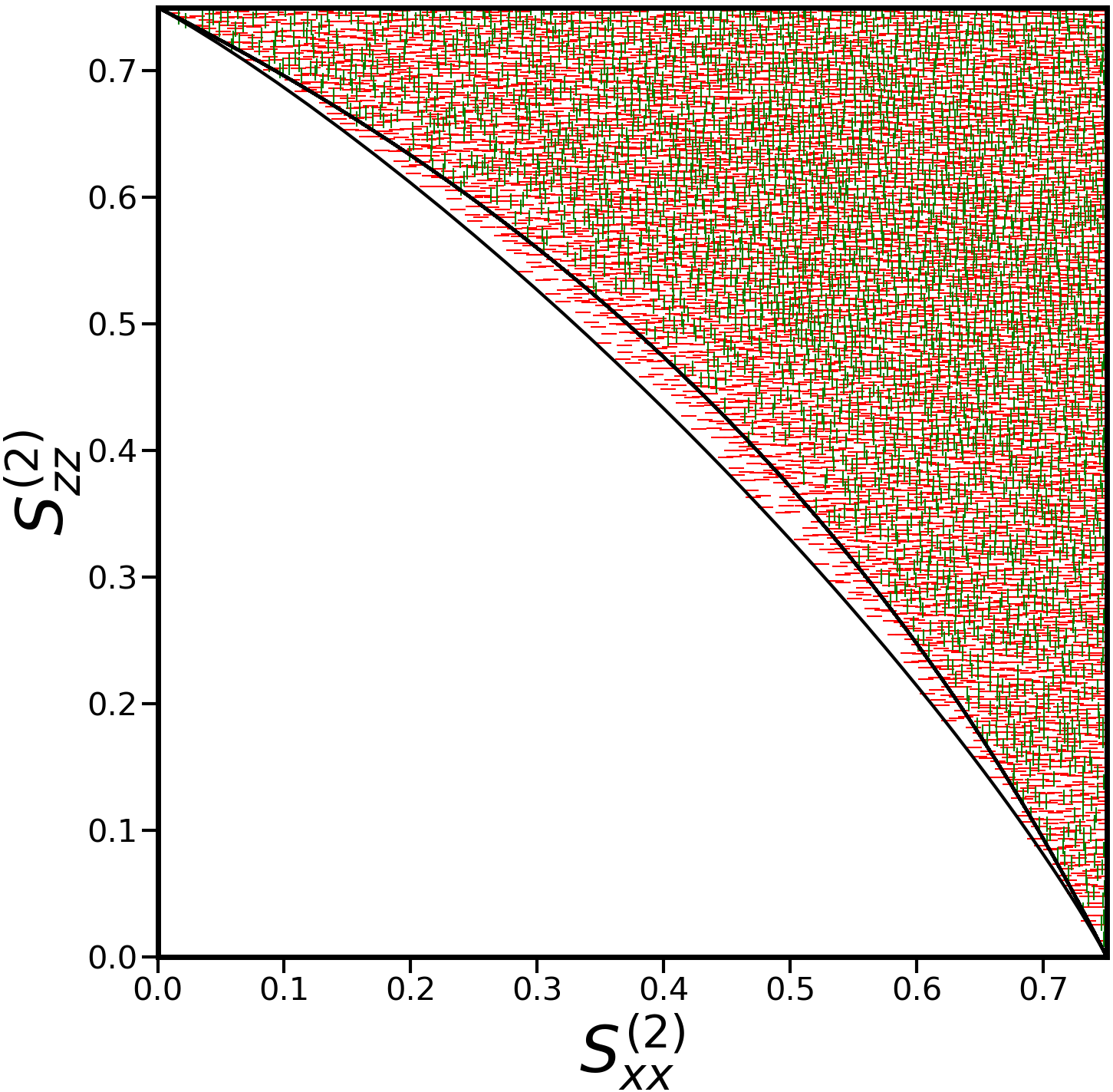
Figure 1: These plots show entropy samples of local measurements $\sigma_{x}\otimes\sigma_{x}$ and $\sigma_{z}\otimes\sigma_{z}$ for Shannon entropy (top) and Tsallis-$2$ entropy (bottom) where separable and entangled states are represented by green vertical and red horizontal lines, respectively. The plot indicates that Shannon entropy is useless for entanglement detection, while Tsallis-$2$ entropy is suitable.

Entropies provide a natural framework to examine scrambled data because they are invariant under permutation of probabilities and hence, robust against scrambling. In this section, we show that measuring Tsallis-$q$ or Rényi-$\alpha$ entropies for the two local measurements $\sigma_{x}\otimes\sigma_{x}$ and $\sigma_{z}\otimes\sigma_{z}$ in many cases allows for the detection of entanglement and show a new family of non-linear, optimal entropic uncertainty relations.

For local measurements $\sigma_{i}\otimes\sigma_{i}$, $S_{ii}$ and $S_{ii}^{(q)}$ where $i\in\{x,y,z\}$ shall denote the Shannon and Tsallis-$q$ entropy of the corresponding four probabilities, respectively. For probabilities $\vec{p}$, they are given by shannon1949 ; havrda1967 ; tsallis1988possible ; wehner2010entropic

$$S(\vec{p}) =-\sum_{j}p_{j}\log p_{j},$$ (1)

$$S^{(q)}(\vec{p}) =\frac{1}{q-1}\Big{(}1-\sum_{j}p_{j}^{q}\Big{)}.$$ (2)

In order to detect entanglement, we investigate the possible pairs of $S_{xx}^{(\tilde{q})}$ and $S_{zz}^{(q)}$ that can be realized by physical states. For gaining some intuition, we have plotted in Fig. 1 random samples of separable and entangled two-qubit states, where separability can be checked using the PPT criterion peres1996separability . As the figures indicate, the accessible region for both kinds of states does not differ in the case of Shannon entropy and hence, entanglement detection seems impossible in this case. This is supported by findings in earlier works: It has been shown in Ref. schwonnek2018additivity that in the case of Shannon entropy and two local measurements, linear entropic uncertainty relations of the type $\alpha S_{xx}+\beta S_{zz}\geq c_{\text{sep}}\geq c$ with bounds $c_{\text{sep}}$ for separable and $c$ for all states, are infeasible to detect entanglement, i.e., $c_{\text{sep}}=c$. Furthermore, Conjecture V.6 in Ref. abdelkhalek2015optimality states that in the example of local measurements $\sigma_{x}\otimes\sigma_{x}$ and $\sigma_{z}\otimes\sigma_{z}$, even non-linear entropic uncertainty relations cannot be used to detect entanglement. However, non-linear relations are unknown in most cases abdelkhalek2015optimality .

In contrast to the case of Shannon entropy, using Tsallis-$2$ entropy, we identify a distinct region occupied by entangled states only, see the lower part of Fig. 1). In the following, we will show that also $(S_{xx}^{(\tilde{q})},S_{zz}^{(q)})$-plots with $q,\tilde{q}\geqslant 2$ exhibit this feature by determining the lower bounds of the set of all and the set of separable states.

In order to obtain the boundary of this realizable region, note first that a vanishing entropy of $S_{ii}^{q}=0$ implies that the system is in an eigenstate of the measurement operator $\sigma_{i}\otimes\sigma_{i}$. Since the measurements define mutually unbiased bases, it is clear that in this case the other entropy is maximal. Hence, the states $\ket{00}$ and $\ket{++}$ lie on the boundary of the realizable region. The mixture of these states with white noise $\mathds{1}/4$ leaves the maximal entropy of one measurement unchanged while increasing the entropy of the other measurement continuously. Therefore, the upper and the right boundary of the region, corresponding to maximal $S_{zz}$ and $S_{xx}$, respectively, is reached by separable states (see Fig. 1). We will see later that the lower boundaries for all and for separable states are both realized by continuous one-parameter families of states. Thus, the mixture of these states with white noise forms a continuous family of curves connecting the lower boundary with the point where both entropies are maximal. Hence, these states realize any accessible point in the entropy plot and it is sufficient to only determine the lower boundary.

III.1 Entropic bound for general states

We begin by determining the bounds in the $(S_{xx}^{(\tilde{q})},S_{zz}^{(q)})$-plot for all states.

In Ref. abdelkhalek2015optimality , Theorem V.2 states that for two concave functionals $f_{1},f_{2}$ on the state space, for any state $\rho$, there is a pure state $\ket{\psi}$ such that $f_{1}(\ket{\psi}\bra{\psi})\leqslant f_{1}(\rho)$ and $f_{2}(\ket{\psi}\bra{\psi})\leqslant f_{2}(\rho)$. Furthermore, it is shown in Theorem V.3 that the state $\ket{\psi}$ can additionally be chosen real if the inputs of the functionals are linked by a real unitary matrix. Thus, in the case of general two-qubit states and local measurements $\sigma_{x}\otimes\sigma_{x}$ and $\sigma_{z}\otimes\sigma_{z}$, the analysis of the boundary of the entropy plots can be reduced to pure real states. First, we will solve the special case where $q=2$, also known as linear entropy. This result can then be used as an anchor to prove the bound for all $q\geqslant 2$.

Lemma 1.

For two-qubit states $\rho$ and fixed $S_{zz}^{(2)}(\rho)$, minimal $S_{xx}^{(2)}(\rho)$ is reached by the unique state $\rho=\ket{\psi_{t}}\bra{\psi_{t}}$ where $\ket{\psi_{t}}=\frac{1}{\sqrt{3+t^{2}}}(t\ket{00}+\ket{01}+\ket{10}+\ket{11})$ and some $t\geqslant 1$ determined by the given entropy $S_{zz}^{(2)}(\rho)$.

Proof.

According to Theorem V.3 in Ref. abdelkhalek2015optimality , if two entropies $S_{1}$ and $S_{2}$ are considered where the measurement bases are related by a real unitary transformation, then for any state $\rho$, there is always a pure and real state $\ket{\psi}$ with $S_{1}(\ket{\psi}\bra{\psi})\leqslant S_{1}(\rho)$ and $S_{2}(\ket{\psi}\bra{\psi})\leqslant S_{2}(\rho)$. As in our case $\sigma_{x}=H\sigma_{z}H^{\dagger}$ where $H$ is the Hadamard matrix, it is sufficient to consider pure real states to obtain minimal $S_{zz}^{(2)}$ for given $S_{xx}^{(2)}$. For a general pure real state $\ket{\psi}=(x_{1},x_{2},x_{3},x_{4})^{T}$, the problem boils down to the following maximization problem under constraints

$$\begin{split}\max_{x_{i}}\>&f(x_{1},x_{2},x_{3},x_{4}),\\ \text{s.t. }&x_{1}^{4}+x_{2}^{4}+x_{3}^{4}+x_{4}^{4}=k=\text{const.},\\ &x_{1}^{2}+x_{2}^{2}+x_{3}^{2}+x_{4}^{2}=1\end{split}$$ (3)

where $f(\{x_{i}\})=(x_{1}+x_{2}+x_{3}+x_{4})^{4}+(x_{1}+x_{2}-x_{3}-x_{4})^{4}+(x_{1}-x_{2}+x_{3}-x_{4})^{4}+(x_{1}-x_{2}-x_{3}+x_{4})^{4}=1-S_{xx}^{(2)}$ and $k=1-S_{zz}^{(2)}$. Note that $\frac{1}{4}\leqslant k\leqslant 1$. It is straightforward to see that $\frac{1}{96}[f(\{x_{i}\})-12\times 1^{2}+8k]=\frac{1}{96}[f(\{x_{i}\})-12(x_{1}^{2}+x_{2}^{2}+x_{3}^{2}+x_{4}^{2})^{2}+8(x_{1}^{4}+x_{2}^{4}+x_{3}^{4}+x_{4}^{4})]=x_{1}x_{2}x_{3}x_{4}$, using the constraints. So, we can replace $f$ by $x_{1}x_{2}x_{3}x_{4}$. Clearly, the $x_{j}$ can be chosen greater than $0$ in case of a maximum. Consequently, $x_{i}$ can be substituted by $\sqrt{y_{i}}$. Because $\sqrt{\cdot}$ is a monotone function, the objective function $y_{1}y_{2}y_{3}y_{4}$ is equivalent to $\sqrt{y_{1}y_{2}y_{3}y_{4}}$ since we are only interested in the state realizing the boundary and not necessarily the boundary itself. Thus, the problem reduces to

$$\begin{split}\max_{y_{i}}\>&y_{1}y_{2}y_{3}y_{4},\\ \text{s.t. }&y_{1}^{2}+y_{2}^{2}+y_{3}^{2}+y_{4}^{2}=k=\text{const.},\\ &y_{1}+y_{2}+y_{3}+y_{4}=1\end{split}$$ (4)

where all $y_{i}$ are positive. Using Lagrange multipliers, one obtains the optimal solution: For given $S_{zz}^{(2)}$, the minimal $S_{xx}^{(2)}$ is reached by the state

$$\ket{\psi_{t}}=\frac{1}{\sqrt{3+t^{2}}}(t\ket{00}+\ket{01}+\ket{10}+\ket{11}),$$ (5)

for some $t\geqslant 1$. Since the minimal $S_{zz}^{(2)}$-entropy state $\ket{\psi_{\infty}}=\ket{00}$ and maximal $S_{zz}^{(2)}$-entropy state $\ket{\psi_{0}}=\frac{1}{2}(\ket{00}+\ket{01}+\ket{10}+\ket{11})$ are part of the family $\ket{\psi_{t}}$ and $\frac{dS_{zz}^{(2)}(\ket{\psi_{t}})}{dt}<0$, fixing $S_{zz}^{(2)}$ uniquely determines $t$ and hence, also $\rho_{t}=\ket{\psi_{t}}\bra{\psi_{t}}$. ∎

This result holds for the Tsallis-2 entropy. However, it can be generalized to any pair of Tsallis-$q$ and Tsallis-$\tilde{q}$ entropies with $q,\tilde{q}\geqslant 2$. To that end, we use a result from Ref. berry2003bounds . There, the authors consider entropy measures $H_{f}=\sum_{i}f(p_{i})$ and $H_{g}=\sum_{i}g(p_{i})$ where $f(0)=g(0)=0$ and the functions $f,g$ are strictly convex (implying that $g^{\prime}(p)$ is invertible) with their first derivatives being continuous in the interval $(0,1)$. They show that then the maximum (minimum) of $H_{f}$ for fixed $H_{g}$ is obtained by the probability distribution $p_{1}\geqslant p_{2}=\dots=p_{n}$ if $f^{\prime}[p(g^{\prime})]$ as a function of $g^{\prime}$ is strictly convex (concave). Furthermore, for each value of $H_{g}$, there is a unique probability distribution of this form.

In the specific case of Tsallis entropies with parameters $q$ and $\tilde{q}$, it is shown that if

$$\frac{q(q-1)}{\tilde{q}(\tilde{q}-1)}p^{q-\tilde{q}}$$ (6)

is monotonically increasing (decreasing), the minimum (maximum) $S^{q}$ for fixed $S^{\tilde{q}}$ is reached by the probability distribution described above, when considering the same measurement for different $q,\tilde{q}$. That is exactly the probability distribution obtained by measuring $\sigma_{x}\otimes\sigma_{x}$ or $\sigma_{z}\otimes\sigma_{z}$ locally in the state $\ket{\psi_{t}}$ since

$$\ket{\psi_{t}} \propto t\ket{00}+\ket{01}+\ket{10}+\ket{11}$$

$$\propto(t+3)\ket{++}+(t-1)(\ket{+-}+\ket{-+}+\ket{--}),$$ (7)

where $t^{2}\geqslant 1$ and $(t+3)^{2}\geqslant(t-1)^{2}$. This observation assists in proving the following theorem:

Figure 2: These sketched plots depict the proof of Theorem 2. Starting with the lower right picture, for fixed $\rho_{r}$ with $S_{xx}^{(\tilde{q})}(\rho_{r})=r$, we consider the state $\ket{\psi_{t_{0}}}$ defined in Lemma 1, with $t_{0}$ such that also $S_{xx}^{(\tilde{q})}(\psi_{t_{0}})=r$. The state $\ket{\psi_{t_{0}}}$ has the largest $S_{xx}^{(2)}$-entropy among all states $\rho$ with $S_{xx}^{(\tilde{q})}(\rho)=r$ berry2003bounds , particularly including $\rho_{r}$ (see lower left). From Lemma 1, it follows that $S_{zz}^{(2)}(\psi_{t_{0}})\leqslant S_{zz}^{(2)}(\rho_{r})$ which is shown in the upper left. This, in turn, implies that $S_{zz}^{(q)}(\psi_{t_{0}})\leqslant S_{zz}^{(q)}(\rho_{r})$ berry2003bounds (see plot on the upper right). In summary, we have for any state $\rho_{r}$ that there exists a state $\ket{\psi_{t_{0}}}$ with $S_{xx}^{(\tilde{q})}(\psi_{t_{0}})=S_{xx}^{(\tilde{q})}(\rho)$ and $S_{zz}^{(q)}(\psi_{t_{0}})\leqslant S_{zz}^{(q)}(\rho)$. This proves that the boundary is realized by the states $\ket{\psi_{t}}$, which is illustrated again in the lower right.

Theorem 2.

For all $q,\tilde{q}\geqslant 2$, the lower boundary in the $(S_{xx}^{(\tilde{q})},S_{zz}^{(q)})$-plot is realized by the family of states $\ket{\psi_{t}}=\frac{1}{\sqrt{3+t^{2}}}(t\ket{00}+\ket{01}+\ket{10}+\ket{11})$ where $t\geqslant 1$.

Proof.

For fixed $r$ and a state $\rho_{r}$ with $S_{xx}^{(\tilde{q})}(\rho_{r})=r$, there exists a unique state $\ket{\psi_{t_{0}}}$ with $S_{xx}^{(\tilde{q})}(\psi_{t_{0}})=r$. From Theorem $1$ in Ref. berry2003bounds , it follows that

$$S_{xx}^{(2)}(\rho_{r})\leqslant S_{xx}^{(2)}(\psi_{t_{0}})\equiv s$$ (8)

(see bottom left graph in Fig. 2). Since $\frac{dS_{zz}^{(2)}(\ket{\psi_{t}})}{dS_{xx}^{(2)}(\ket{\psi_{t}})}=\frac{dS_{zz}^{(2)}(\ket{\psi_{t}})}{dt}\left(\frac{dS_{xx}^{(2)}(\ket{\psi_{t}})}{dt}\right)^{-1}<0$, it follows from Lemma 1 that $S_{xx}^{(2)}(\rho_{r})\leqslant s$ implies

$$S_{zz}^{(2)}(\rho_{r})\geqslant S_{zz}^{(2)}(\psi_{t_{0}})\equiv u$$ (9)

(see top left graph in Fig. 2). Now, given $S_{zz}^{(2)}(\rho_{r})\geqslant u$, using the fact that $\frac{dS_{zz}^{(q)}(\ket{\psi_{t}})}{dS_{zz}^{(2)}(\ket{\psi_{t}})}>0$, it follows from Ref. berry2003bounds that

$$S_{zz}^{(q)}(\rho_{r})\geqslant S_{zz}^{(q)}(\psi_{t_{0}})\equiv v$$ (10)

(see top right graph in Fig. 2).

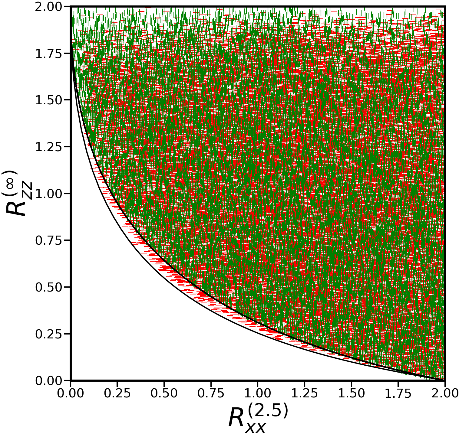
Figure 3: This plots shows entropy samples of local measurements $\sigma_{x}\otimes\sigma_{x}$ and $\sigma_{z}\otimes\sigma_{z}$ for Rényi-$2.5$- and Rényi-$\infty$-entropies, respectively. Separable states are represented by green vertical lines, while red horizontal lines indicate entangled states. The lower boundary is given by the states $\ket{\psi_{t}}$ defined in Lemma 1.

In summary, by considering all values of $r$, we found that for all two-qubit states $\rho_{r}$,

$$S_{xx}^{(\tilde{q})}(\rho_{r})=r \Rightarrow S_{xx}^{(2)}(\rho_{r})\leqslant S_{xx}^{(2)}(\psi_{t_{0}})$$ (11)

$$\Rightarrow S_{zz}^{(2)}(\rho_{r})\geqslant S_{zz}^{(2)}(\psi_{t_{0}})$$ (12)

$$\Rightarrow S_{zz}^{(q)}(\rho_{r})\leqslant S_{zz}^{(q)}(\psi_{t_{0}})$$ (13)

(see also the lower right graph in Fig. 2), where $\ket{\psi_{t_{0}}}$ is uniquely determined by $S_{xx}^{(\tilde{q})}(\psi_{t_{0}})=r$. All bounds, as well as the overall implication $S_{xx}^{(\tilde{q})}(\rho_{r})=r\Rightarrow S_{zz}^{(q)}(\rho_{r})\leqslant S_{zz}^{(q)}(\psi_{t_{0}})$ are tight since they are saturated by the same state $\ket{\psi_{t_{0}}}$. Thus, the lower boundary in the $(S_{xx}^{(\tilde{q})},S_{zz}^{(q)})$-plot is realized by the family of states $\ket{\psi_{t}}=\frac{1}{\sqrt{3+t^{2}}}(t\ket{00}+\ket{01}+\ket{10}+\ket{11})$ where $t\geqslant 1$. ∎

In the above proof, we used the $q=\tilde{q}=2$-case as an anchor to derive the result for all $q,\tilde{q}\geqslant 2$. The same argument also holds if we would use any other anchor case where the $\ket{\psi_{t}}$ are the optimal states. Numerical evidence suggests that the conclusion is indeed valid for any $q,\tilde{q}\gtrsim 1.37$. Furthermore, the result can also be interpreted as a family of entropic uncertainty relations.

Corollary 3.

For all two-qubit states $\rho$ and $q,\tilde{q}\geqslant 2$,

$$F[S_{xx}^{(\tilde{q})}(\rho),S_{zz}^{(q)}(\rho)]\equiv S_{zz}^{(q)}(\rho)-S_{zz}^{(q)}(\ket{\psi_{t}}[S_{xx}^{(\tilde{q})}(\rho)])$$

$$=S_{zz}^{(q)}(\rho)-\frac{1}{q-1}\left(1-\frac{3+t^{2q}[S_{xx}^{(\tilde{q})}(\rho)]}{\{3+t^{2}[S_{xx}^{(\tilde{q})}(\rho)]\}^{q}}\right)\geqslant 0.$$ (14)

Here, $\ket{\psi_{t}}[S_{xx}^{(\tilde{q})}(\rho)]$ and $t[S_{xx}^{(\tilde{q})}(\rho)]$ are the unique state $\ket{\psi_{t}}$ and parameter $t$ in dependence on $S_{xx}^{(\tilde{q})}(\rho)$, such that $S_{xx}^{(\tilde{q})}(\ket{\psi_{t}})=S_{xx}^{(\tilde{q})}(\rho)$.

For the example of $q=\tilde{q}=2$, we have

$$F[S_{xx}^{(2)}(\rho),S_{zz}^{(2)}(\rho)]=S_{zz}^{(2)}-\frac{3QT^{2}-T^{4}}{3Q^{2}}\geqslant 0,$$ (15)

where

$$T =\sqrt{9-12S_{xx}^{(2)}},$$ (16)

$$Q =3+T+\sqrt{3}\sqrt{(1+T)(3-T)}.$$ (17)

This bound is displayed in Fig. 1.

Note that this result is also valid for Rényi-$\alpha$ entropies renyi1961proceedings with $\alpha,\tilde{\alpha}\geqslant 2$ as Rényi-$\alpha$ and Tsallis-$q$ entropies are monotone functions of each other for $\alpha=q$. Thus, the change from the Tsallis- to the Rényi entropy induces simply a rescaling of the axis in the $(S_{xx},S_{zz})$-plot. An example is given in Fig. 3 where $\alpha=2.5$ and $\tilde{\alpha}=\infty$.

In contrast to any linear bounds, which are usually considered schwonnek2018additivity , the uncertainty relations found here are optimal. That means, for any entropic uncertainty relation defined in Corollary 3 and any $S_{zz}^{(q)}$, there exists a state, namely the $\ket{\psi_{t}}$ with the given entropy, saturating the corresponding bound.

III.2 Entropic bound for separable states

In this section, we determine the bound for separable states. Theorem V.2 from Ref. abdelkhalek2015optimality , which shows that for any state $\rho$ there is a pure state $\ket{\psi}$ such that $f_{1}(\psi)\leqslant f_{1}(\rho)$ and $f_{2}(\psi)\leqslant f_{2}(\rho)$, cannot be applied to separable states. This is because the boundary of the space of separable states is determined by positivity as well as separability conditions. While the former implies that states on the boundary are of lower rank, the latter gives a different constraint. However, this can still be used to simplify the optimization process, as we prove in the following:

Theorem 4.

Let $f_{1}$, $f_{2}$ be two continuous concave functions on the state space. Then, for every separable state $\rho$, there exists a separable state $\rho^{*}$ of the form

$$\rho^{*}=(1-p)\ket{ab}\bra{ab}+p\ket{cd}\bra{cd},$$ (18)

where $0\leqslant p\leqslant 1$ and $\ket{ab}\bra{ab}$, $\ket{cd}\bra{cd}$ are pure product states, such that $f_{1}(\rho^{*})\leqslant f_{1}(\rho)$ and $f_{2}(\rho^{*})\leqslant f_{2}(\rho)$.

Proof.

In the range of $\rho$, we consider some state $\sigma$ on the boundary of the space of separable states in this subspace. Then, there is some antipode $\sigma^{\blacktriangledown}$ defined as $\frac{1}{\lambda}\left[\rho-(1-\lambda)\sigma\right]$ for the smallest $\lambda$ such that this expression still describes a separable state. By this definition, obviously, also $\sigma^{\blacktriangledown}$ lies on the boundary. Now, $\sigma$ can be converted continuously into $\sigma^{\blacktriangledown}$ by a curve $t\mapsto\gamma(t)$ on the boundary where $\gamma(0)=\sigma$ and $\gamma(1)=\sigma^{\blacktriangledown}$, as long as the boundary is connected (see Fig.4). Since the functions are continuous, there must be some $t^{*}\in[0,1]$ such that $f_{1}[\gamma(t^{*})]=f_{1}(\rho)$. At this point, either $f_{2}[\gamma(t^{*})]\leqslant f_{2}(\rho)$ or it holds that $f_{1}[\gamma^{\blacktriangledown}(t^{*})]\leqslant f_{1}(\rho)$ and $f_{2}[\gamma^{\blacktriangledown}(t^{*})]\leqslant f_{2}(\rho)$ since otherwise concavity implies the contradiction

$$f_{i}(\rho) \geqslant[1-\lambda(t)]f_{i}[\gamma(t)]+\lambda(t)f_{i}[\gamma^{\blacktriangledown}(t)]$$ (19)

$$>[1-\lambda(t)]f_{i}(\rho)+\lambda(t)f_{i}(\rho)=f_{i}(\rho)$$ (20)

for $i=1$ or $i=2$. Thus, we find a state $\gamma^{*}$ with $f_{1,2}[\gamma^{*}]\leqslant f_{1,2}(\rho)$. Compared to $\rho$, this boundary state $\gamma^{*}$ satisfies at least one additional constraint of the form

$$\gamma^{*}\ket{\phi_{0}}=0, \operatorname{Tr}(\gamma^{*}W)=0,$$ (21)

where $\ket{\phi_{0}}$ is an eigenstate of $\gamma^{*}$ and $W$ is an entanglement witness, because $\gamma^{*}$ lies at the positivity or separability boundary, respectively.

When we decompose $\gamma^{*}$ into pure product states $\gamma^{*}=\sum_{j}p_{j}\ket{a_{j}b_{j}}\bra{a_{j}b_{j}}$, every $\ket{a_{j}b_{j}}\bra{a_{j}b_{j}}$ satisfies the constraints individually. This is because the range of each of them has to be contained in the range of $\gamma^{*}$. Furthermore, for product states it holds that $\operatorname{Tr}(\ket{a_{j}b_{j}}\bra{a_{j}b_{j}}W)\geqslant 0$ and since we have $0=\operatorname{Tr}(\gamma^{*}W)=\sum_{j}p_{j}\operatorname{Tr}(\ket{a_{j}b_{j}}\bra{a_{j}b_{j}}W)$, also $\operatorname{Tr}(\ket{a_{j}b_{j}}\bra{a_{j}b_{j}}W)=0$.

Thus, we can apply this procedure repeatedly, considering only the state space defined by the already accumulated constraints of the form given in Eq. (21). In the end, we either have a pure product state $\rho^{*}$ or a one-dimensional state space spanned by two pure product states $\ket{ab}\bra{ab}$ and $\ket{cd}\bra{cd}$, whose boundary is disconnected and hence, the scheme cannot be applied anymore. This might indeed happen, as there are two-dimensional subspaces of the two-qubit space with exactly two product vectors in it sanpera1998local . Either way, for any separable state $\rho$ we find a state $\rho^{*}$ of the form $\rho^{*}=(1-p)\ket{ab}\bra{ab}+p\ket{cd}\bra{cd}$ such that $f_{1}(\rho^{*})\leqslant f_{1}(\rho)$ and $f_{2}(\rho^{*})\leqslant f_{2}(\rho)$. ∎

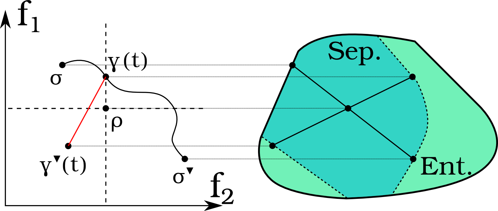
Figure 4: This sketch shows the proof idea of Theorem 4, where the left plot is based on Fig. 6 in Ref. abdelkhalek2015optimality . Any separable state $\rho$ can be written as the mixture of two states on the topological boundary of the space of separable states. These two states can be converted into each other continuously. In this process, we find a state $\gamma^{\blacktriangledown}(t)$ on the boundary such that $f_{1}[\gamma^{\blacktriangledown}(t)]\leqslant f_{1}(\rho)$ and $f_{2}[\gamma^{\blacktriangledown}(t)]\leqslant f_{2}(\rho)$ for continuous concave functionals $f_{1}$ and $f_{2}$.

In the case of local $\sigma_{x}\otimes\sigma_{x}$ and $\sigma_{z}\otimes\sigma_{z}$ measurements, we can restrict the optimization further to real states $\ket{ab}$ and $\ket{cd}$.

Observation 5.

For any separable state $\rho$, there is a state $\rho^{*}=(1-p)\ket{ab}\bra{ab}+p\ket{cd}\bra{cd}$ where $0\leqslant p\leqslant 1$ and $\ket{ab}$ and $\ket{cd}$ are pure and real product states such that $S_{xx}^{(\tilde{q})}(\rho^{*})\leqslant S_{xx}^{(\tilde{q})}(\rho)$ and $S_{zz}^{(q)}(\rho^{*})\leqslant S_{zz}^{(q)}(\rho)$ for any $q,\tilde{q}\in\mathds{R}$.

Proof.

Using Theorem 4, we immediately find a state $\sigma=(1-p)\ket{ab}\bra{ab}+p\ket{cd}\bra{cd}$ such that $S_{xx}^{(\tilde{q})}(\sigma)\leqslant S_{xx}^{(\tilde{q})}(\rho)$ and $S_{zz}^{(q)}(\sigma)\leqslant S_{zz}^{(q)}(\rho)$ for any $q,\tilde{q}\in\mathds{R}$. However, the states $\ket{ab}$ and $\ket{cd}$ might not be real.

A general one-qubit state can be written as $\ket{a}=\cos\frac{\theta}{2}\ket{0}+e^{i\varphi}\sin\frac{\theta}{2}\ket{1}$ where $0\leqslant\theta\leqslant\pi$ and $0\leqslant\varphi<2\pi$. The corresponding probabilities for $\sigma_{x}$ and $\sigma_{z}$ measurements are then given by

$$p_{0} =\cos^{2}\frac{\theta}{2}\text{, }p_{1}=\sin^{2}\frac{\theta}{2},$$ (22)

$$p_{\pm} =\frac{1}{2}\pm\frac{1}{2}\sin\theta\cos\varphi.$$ (23)

Hence, by just varying $\varphi$, $p_{0}$ and $p_{1}$ remain unaffected, while $p_{+}=(1-\alpha)P_{\text{max}}+\alpha P_{\text{min}}$ and $p_{-}=\alpha P_{\text{max}}+(1-\alpha)P_{\text{min}}$, where $P_{\text{max}}=\frac{1}{2}+\frac{1}{2}\sin\theta$ and $P_{\text{max}}=\frac{1}{2}-\frac{1}{2}\sin\theta$, vary continuously with $0\leqslant\alpha\leqslant 1$. Now, consider varying the state $\ket{a}$ in such a way while leaving $\ket{b}$ and $\ket{cd}$ the same. Obviously, the probability distribution for the $\sigma_{z}\otimes\sigma_{z}$ measurement on $\sigma$ stays unchanged. The $\sigma_{x}\otimes\sigma_{x}$ measurement, on the other hand, yields $(1-\alpha)\vec{p_{1}}+\alpha\vec{p_{2}}$ for some probability distributions $\vec{p_{1}}$ and $\vec{p_{2}}$. Hence, the optimization problem over $\alpha$ is an optimization over a convex set of probabilities. As the entropies are concave functions of probability distributions, the optimum can be found at the boundary. Note that we only optimize the $S_{xx}^{\tilde{q}}$ while leaving $S_{zz}^{q}$ unchanged. Thus, $\ket{a}$ can be chosen real and so can $\ket{b}$, $\ket{c}$ and $\ket{d}$. ∎

Reducing the optimization to real states of rank at most two, the lower number of parameters allows for robust numerical analysis. This suggests that for $q,\tilde{q}\geqslant 2$, the boundary is reached by real pure product states of the form

$$\ket{\phi^{q,\tilde{q}}_{\theta}}=\Big{(}\cos\frac{\theta}{2}\ket{0}+\sin\frac{\theta}{2}\ket{1}\Big{)}^{\otimes 2}.$$ (24)

For $q=\tilde{q}=2$, we obtain the (numerical) boundary for separable states $\rho$ as

$$S_{zz}^{(2)}(\rho)\geqslant-\frac{9}{4}+3\sqrt{1-S_{xx}^{(2)}(\rho)}+S_{xx}^{(2)}(\rho),$$ (25)

which is shown in Fig. 1. In the case of Shannon entropy, numerical analysis indicates that the boundary is realized by the states

$$\ket{\phi^{S}_{\theta}} =\ket{0}\otimes\Big{(}\cos\frac{\theta}{2}\ket{0}+\sin\frac{\theta}{2}\ket{1}\Big{)},$$ (26)

$$\ket{\psi^{S}_{\theta}} =\Big{(}\cos\frac{\theta}{2}\ket{0}+\sin\frac{\theta}{2}\ket{1}\Big{)}\otimes\ket{+},$$ (27)

which is also shown in Fig. 1.

III.3 Robustness

In the previous sections, we showed that the accessible regions in the entropy plot $(S^{(q)}_{xx},S^{(\tilde{q})}_{zz})$ are different for general two-qubit states and separable states when $q,\tilde{q}\geqslant 2$. Thus, these entropies provide a scrambling-invariant method to detect entanglement. The accessible regions for $q=\tilde{q}=2$ are shown in Fig. 1.

We investigate the robustness of this detection method for different $q=\tilde{q}\geqslant 2$. The robustness is quantified by the amount of white noise that can be added to the boundary states defined in Eq. (5) such that they are still detectable. Numerical analysis indicates that independent of $q$, the most robust states are those with $S^{(q)}_{xx}=S^{(q)}_{zz}$, i.e. $t=3$. For states $\rho_{\lambda,t}=(1-\lambda)\ket{\psi_{t}}\bra{\psi_{t}}+\lambda\frac{\mathds{1}}{4}$, it also holds that $S^{(q)}_{xx}(\rho_{\lambda,t})=S^{(q)}_{zz}(\rho_{\lambda,t})$ independent of $\lambda$ and hence, they enter the region of separable states at the point of the symmetric real pure product state $\big{[}\frac{1}{\sqrt{1+s^{2}}}(s\ket{0}+\ket{1})\big{]}^{\otimes 2}$ where $s=1+\sqrt{2}$. The maximal noise level $\lambda$ is then determined by

$$\begin{split}&\Big{(}\frac{(1-\lambda)t}{\sqrt{3+t^{2}}}+\frac{\lambda}{4}\Big{)}^{2q}+3\Big{(}\frac{(1-\lambda)}{\sqrt{3+t^{2}}}+\frac{\lambda}{4}\Big{)}^{2q}\\ &=\Big{(}\frac{s^{2}}{1+s^{2}}\Big{)}^{2q}+2\Big{(}\frac{s}{1+s^{2}}\Big{)}^{2q}+\Big{(}\frac{1}{1+s^{2}}\Big{)}^{2q}\end{split}$$ (28)

which can be solved analytically for large $q$. In the limit of $q\rightarrow\infty$, $\lambda=\frac{1}{11}(10-\sqrt{2}-\sqrt{12}-\sqrt{24})\approx 0.020$. Note that this is an upper bound on the robustness, since the boundary of the region of separable states was only determined numerically in the last section. However, even this upper bound is rather small and the method is not very robust. Finally, we see that the method is most robust for large $q$, but the limit is reached very fast.

IV Scrambling-invariant families of entanglement witnesses

A powerful method of detecting entanglement in the usual scenario are entanglement witnesses. An entanglement witness $W$ is a hermitian operator with non-negative expectation values for all separable states, and a negative expectation value for some entangled state $\rho$ guhne2009entanglement . We say that $W$ detects $\rho$, as $\langle W\rangle_{\rho}<0$ proves that $\rho$ is entangled. In this section, we show how witnesses can be used in the scrambled data scenario.

IV.1 Scrambling-invariant witnesses

Inspired by the probability distributions of the states defined in Eq. (5), we define a scrambling-invariant family of entanglement witnesses. In the most general form, with local measurements $\sigma_{x}\otimes\sigma_{x}$, $\sigma_{y}\otimes\sigma_{y}$, and $\sigma_{z}\otimes\sigma_{z}$, they are given by

$$\begin{split}W=\hskip 3.0pt&\mathds{1}+\alpha\ket{x_{1}x_{2}}\bra{x_{1}x_{2}}\\ &+\beta\ket{y_{1}y_{2}}\bra{y_{1}y_{2}}+\gamma\ket{z_{1}z_{2}}\bra{z_{1}z_{2}},\end{split}$$ (29)

where $\ket{x_{j}}\in\{\ket{+},\ket{-}\}$, $\ket{y_{j}}\in\{\ket{\text{y}^{+}},\ket{\text{y}^{-}}\}$, and $\ket{z_{j}}\in\{\ket{0},\ket{1}\}$ for $j=1,2$.

The key observation is that if for fixed $\alpha$, $\beta$ and $\gamma$ this yields an entanglement witness, then also every other choice of $x_{j}$, $y_{j}$ and $z_{j}$ results in an entanglement witness. This is because using only local unitary transformations and the partial transposition, the witnesses can be transformed into each other. Consider for example $W=\mathds{1}+\alpha\ket{+-}\bra{+-}+\beta\ket{\text{y}^{+}\text{y}^{+}}\bra{\text{y}^{+}\text{y}^{+}}+\gamma\ket{10}\bra{10}$, and the transformations $U_{A}=\sigma_{x}$, and $U_{B}=\mathds{1}$. Then, $U_{A}^{\dagger}\otimes U_{B}^{\dagger}W^{T_{A}}U_{A}\otimes U_{B}=\mathds{1}+\alpha\ket{+-}\bra{+-}+\beta\ket{\text{y}^{+}\text{y}^{+}}\bra{\text{y}^{+}\text{y}^{+}}+\gamma\ket{00}\bra{00}$ and one can directly check that any other witness can also be reached.

Indeed, such mappings correspond to permutations of the probabilities, as

$$\langle W\rangle=1+\alpha p_{x_{1}x_{2}}+\beta p_{y_{1}y_{2}}+\gamma p_{z_{1}z_{2}}.$$ (30)

So, for evaluating such a witness from scrambled data, one can just choose the probabilities appropriately in order to minimize the mean value of the witness.

As a remark, for $\alpha,\beta,\gamma<0$, the witnesses are additionally related to an entropic uncertainty relation for min-entropy $S^{\infty}(\vec{p})=-\log\max_{j}p_{j}$ since the smallest expectation value of the corresponding family of entanglement witnesses can be written as

$$\langle W\rangle=1+\alpha e^{-S^{(\infty)}_{xx}(\rho)}+\beta e^{-S^{(\infty)}_{yy}(\rho)}+\gamma e^{-S^{(\infty)}_{zz}(\rho)}.$$ (31)

IV.2 Optimized witnesses

We want to find optimized $\alpha$, $\beta$ and $\gamma$ such that $W$ is an entanglement witness tangent to the space of separable states, i.e., there exists a separable state with $\langle W\rangle=0$. In the following analysis, we restrict ourselves to only two measurements and witnesses of the form

$$W=\mathds{1}+\alpha\ket{++}\bra{++}+\gamma\ket{00}\bra{00}.$$ (32)

First of all, we need to ensure that $\langle W\rangle\geqslant 0$ for all separable states. In order to obtain an optimal witness, we further need to adjust $\alpha$ and $\gamma$ such that for some separable state $\langle W\rangle=0$.

The optimal values for $\alpha$ and $\gamma$ are found by optimizing

$$\min_{\rho_{s}}\operatorname{Tr}(\rho_{s}W)$$ (33)

for all $\alpha$ and $\gamma$. Because of linearity, we only need to consider general pure product states $\ket{\psi_{A}}\otimes\ket{\psi_{B}}$ where

$$\ket{\psi_{A/B}}=\cos\frac{\theta_{A/B}}{2}\ket{0}+e^{i\phi_{A/B}}\sin\frac{\theta_{A/B}}{2}\ket{1}$$ (34)

with $0\leqslant\theta\leqslant\pi$, $0\leqslant\phi<2\pi$. It turns out that for $\frac{\gamma}{\alpha}\geqslant-3-2\sqrt{2}$, the optimal state is given by $\phi_{A}=\phi_{B}=0$ and $\theta_{A}=\theta_{B}$, while $\phi_{A}=\phi_{B}=0$ and $\theta_{A}-\frac{3\pi}{4}=\frac{3\pi}{4}-\theta_{B}$ needs to be considered in the case of $\frac{\gamma}{\alpha}\leqslant-3-2\sqrt{2}$.

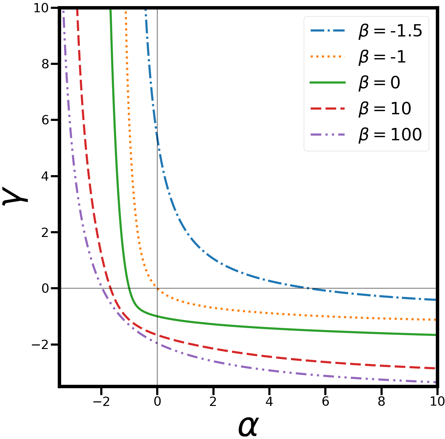
Figure 5: Optimized values for the parameters $\alpha$ and $\gamma$ for different $\beta$ in entanglement witnesses of the form $W=\mathds{1}+\alpha\ket{x_{1}x_{2}}\bra{x_{1}x_{2}}+\beta\ket{y_{1}y_{2}}\bra{y_{1}y_{2}}+\gamma\ket{z_{1}z_{2}}\bra{z_{1}z_{2}}$. Here, optimized means that for some separable state $\langle W\rangle=0$.

Finally, we have to ensure that there exist entangled states with $\langle W\rangle<0$. Since $\langle W\rangle=1+\alpha p_{++}+\gamma p_{00}$ and the probabilities are non-negative, either $\alpha$ or $\gamma$ must necessarily be negative. In that case, the eigenvector of $W$ corresponding to the smallest eigenvalue is indeed given by the entangled state $\ket{\psi_{t}}=\frac{1}{\sqrt{3+t^{2}}}(t,1,1,1)^{T}$ with $t=-{(\alpha-2\gamma+2\sqrt{\alpha^{2}-\alpha\gamma+\gamma^{2}})}/{\alpha}$.

The resulting curve of optimal $\alpha$ and $\gamma$ in the case of $\beta=0$ can thus be obtained analytically and is shown in Fig. 5. More generally, for witnesses of the form in Eq. (29) where $\beta\neq 0$, we find the optimal parameters numerically.

V Non-convex structure of the non-detectable state space

For many methods of entanglement detection, it is crucial that the set of separable states is convex. For instance, the existence of a witness for any entangled state $\rho$ relies on this fact. This convexity is also present in the case of restricted measurements, which are not tomographically complete. If there is a way to detect the entanglement from a restricted set of measurements, it can be done with an entanglement witness curty2005detecting . In this section, we show that this is not the case when only scrambled data is available.

In order to test whether there would in principle be a method to detect the entanglement of a specific state using only scrambled data from local measurements $\sigma_{x}\otimes\sigma_{x}$ and $\sigma_{z}\otimes\sigma_{z}$, we use the fact that the PPT criterion is necessary and sufficient in the two-qubit case horodecki1996ppt . Thus, we can formulate the problem as a family of semi-definite programs (SDPs) boyd . We consider the problem

$$\min_{\rho} 0$$ (35)

s.t. $$\operatorname{Tr}\rho=1,$$

$$\rho\geqslant 0,$$

$$\rho^{T_{B}}\geqslant 0,$$

$$\rho\text{ realizes one of the }(4!)^{2}\text{ permutations}$$

      of the given probability distribution

$$\text{\,\,\,\,\, for measurements }\sigma_{x}\otimes\sigma_{x}\text{ and }\sigma_{z}\otimes\sigma_{z}.$$

This is a so called feasibility problem: If a $\rho$ with the desired properties exist, the output of the SDP is zero, and $\infty$ otherwise. If this family of SDPs fails for all permutations, then there is no separable state that realizes the same scrambled data as the original state. Hence, the entanglement of such a state is detected. Otherwise, we call the state possibly separable.

In practice, without scrambled data, around $1.2\%$ of all random states according to the Hilbert-Schmidt measure can be shown to be entangled using only local measurements $\sigma_{x}\otimes\sigma_{x}$ and $\sigma_{z}\otimes\sigma_{z}$. In the case of scrambled data, we tested approximately $130,000,000$ random mixed states and found around $3000$ detectable states using the corresponding scrambled data. Note that for the implementation it is possible to reduce the number of permutations that need to be considered to just $18$, as local relabeling of the outcomes or the exchange of qubits can be neglected.

Out of these states, only six can be detected using the scrambling-invariant entanglement witnesses and none using the entropic uncertainty relations where $q=\tilde{q}$. The reason for this poor performance is the non-convex structure of the set of non-detectable states, as we discuss now.

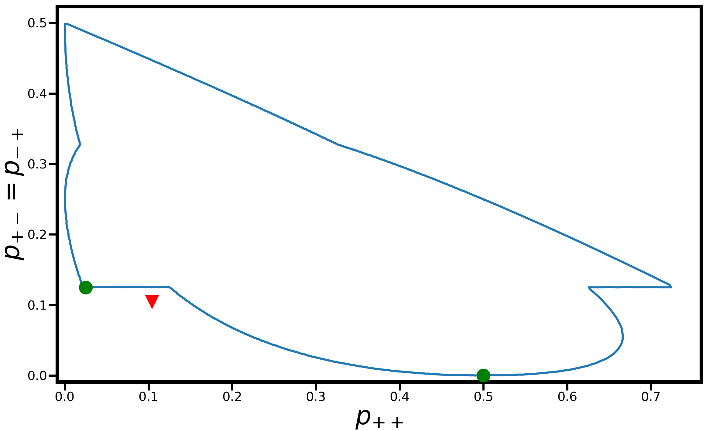
Figure 6: Projection of the set of possibly separable states (blue line) for local measurements $\sigma_{x}\otimes\sigma_{x}$ and $\sigma_{z}\otimes\sigma_{z}$, where $p_{++}=p_{00}$, $p_{+-}=p_{-+}=p_{01}=p_{10}$, and $p_{--}=p_{11}$, onto the coordinates $(p_{++},p_{+-})$. Clearly, this set is non-convex. The green dots and the red triangle correspond to an explicit counterexample to the convexity, as explained in the main text.

First, we note that the set of possibly separable states is star-convex around the maximally mixed state $\frac{\mathds{1}}{4}$. This can be seen as follows: If a state $\rho$ is part of the set of possibly separable states, there is a separable state $\sigma$ that realizes the same probability distribution as $\rho$ up to a permutation. Then, $\lambda\sigma+(1-\lambda)\frac{\mathds{1}}{4}$ is still separable for $0\leqslant\lambda\leqslant 1$ and realizes the same probability distribution as $\lambda\rho+(1-\lambda)\frac{\mathds{1}}{4}$ up to the same permutation as before.

This fact can be used to characterize the boundary of the possibly-separable state space by starting with the maximally mixed state and mixing it with detectable states until the mixture becomes detectable. To illustrate the non-convexity of this set, we assume first that it is convex. Then, the intersection with any convex set, for example the set of states with probabilities $p_{++}=p_{00}$, $p_{+-}=p_{-+}=p_{01}=p_{10}$, and $p_{--}=p_{11}$, would again form a convex set. Furthermore, the projection onto the coordinates $(p_{++},p_{+-})$ would be convex. This projection is shown in Fig. 6. Clearly, it is non-convex, and hence, the initial assumption is incorrect. To make this statement independent of numerical analysis, we provide an explicit counterexample.

Observation 6.

The set of possibly separable states for local measurements $\sigma_{x}\otimes\sigma_{x}$ and $\sigma_{z}\otimes\sigma_{z}$ is non-convex.

The states $\rho_{1}=\frac{1}{4}\left(\mathds{1}\otimes\mathds{1}-\frac{7}{10}(\mathds{1}\otimes\sigma_{x}+\sigma_{x}\otimes\mathds{1}\right.$ $\left.+\mathds{1}\otimes\sigma_{z}+\sigma_{z}\otimes\mathds{1})+\frac{1}{2}(\sigma_{x}\otimes\sigma_{x}+\sigma_{z}\otimes\sigma_{z}+\sigma_{x}\otimes\sigma_{z}\right.$ $\left.+\sigma_{z}\otimes\sigma_{x})\right)$ and $\rho_{2}=\ket{\Phi^{+}}\bra{\Phi^{+}}$ where $\ket{\Phi^{+}}=\frac{1}{\sqrt{2}}(\ket{00}+\ket{11})$ realize probability distributions corresponding to the left and right green dot in Fig. 6, respectively. While $\rho_{1}$ is separable, the product state $\ket{+}\ket{0}$ realizes the same scrambled data as $\rho_{2}$ and hence, $\rho_{2}$ is possibly separable. Thus, they are part of the possibly separable state space. However, the mixture $\rho=\frac{5}{6}\rho_{1}+\frac{1}{6}\rho_{2}$, shown as a red triangle in Fig. 6, is detectable. The scrambled data of the corresponding probability distribution $p_{++}=p_{+-}=p_{-+}=p_{00}=p_{01}=p_{10}=\frac{5}{48}$ and $p_{--}=p_{11}=\frac{33}{48}$ cannot origin from a separable state. The witnesses $W=\mathds{1}\pm\sigma_{x}\otimes\sigma_{x}\pm\sigma_{z}\otimes\sigma_{z}$ certify the entanglement for all permutations.

For general two-qubit states, the same procedure can be applied. Indeed, mixing the $3000$ random detectable states with white noise such that they are barely compatible with scrambled data from separable states, can be used to characterize the boundary of the set of possibly separable states. Mixing pairs of these states with equal weights leads in some cases to detectable states, also witnessing the non-convex structure.

VI Conclusion

We have introduced the concept of scrambled data, meaning that the assignment of probabilities to outcomes of the measurements is lost. Clearly, this restriction limits the possibilities of entanglement detection. Nevertheless, we have shown that using entropies and entanglement witnesses one can still detect the entanglement in some cases. These methods are limited, however, as the set of states whose scrambled data can be realized by separable states is generally not convex.

There are several directions in which our work may be extended or generalized. First, one may consider more general scenarios than the two-qubit situation considered here, such as the case of three or more particles. Second, it would be interesting to study our results on entropies further, in order to derive systematically entropic uncertainty relations for various entropies. Such entropic uncertainty relations find natural applications in the security analysis of quantum key distribution and quantum information theory. Finally, it would be intriguing to connect our scenario to Bell inequalities. This could help to relax assumptions on the data for non-locality detection and device-independent quantum information processing.

VII Acknowledgments

We thank Xiao-Dong Yu, Ana Cristina Sprotte Costa and Roope Uola for fruitful discussions. This work was supported by the DFG, the ERC (Consolidator Grant No. 683107/TempoQ), the Asian Office of Aerospace (R&D grant FA2386-18-1-4033) and the House of Young Talents Siegen.

References

- (1) M. Seevinck and J. Uffink, Phys. Rev. A 76, 042105 (2007).
- (2) N. J. Beaudry, T. Moroder, and N. Lütkenhaus, Phys. Rev. Lett. 101, 093601 (2008).
- (3) J.-D. Bancal, N. Gisin, Y.-C. Liang, and S. Pironio, Phys. Rev. Lett. 106, 250404 (2011).
- (4) T. Moroder and O. Gittsovich, Phys. Rev. A 85, 032301 (2012).
- (5) J. T. Barreiro, J.-D. Bancal, P. Schindler, D. Nigg, M. Hennrich, T. Monz, N. Gisin, and R. Blatt, Nat. Phys. 9, 559 (2013).
- (6) M. A. Rowe, D. Kielpinski, V. Meyer, C. A. Sackett, W. M. Itano, C. Monroe, and D. J. Wineland, Nature 409, 791 (2001).
- (7) O. Gühne and G. Tóth, Phys. Rep. 474, 1 (2009).
- (8) S. Brierley, S. Weigert, and I. Bengtsson, Quant. Inf. Comp. 10, 803 (2010).
- (9) C. Shannon, and W. Weaver, The Mathematical Theory of Communication. University of Illinois Press, Urbana (1949).
- (10) J. Havrda and F. Charvat, Kybernetika 3, 30 (1967).
- (11) C. Tsallis, J. Stat. Phys. 52, 479 (1988).
- (12) S. Wehner and A. Winter, New J. Phys. 12, 25009 (2010).
- (13) A. Peres, Phys. Rev. Lett. 77, 1413 (1996).
- (14) R. Schwonnek, Quantum 2, 59 (2018).
- (15) K. Abdelkhalek, R. Schwonnek, H. Maassen, F. Furrer, J. Duhme, P. Raynal, B.-G. Englert, and R. F. Werner, Int. J. Quantum Inf. 13, 1550045 (2015).
- (16) D. W. Berry, and B. C. Sanders, J. Phys. A 36, 12255 (2003).
- (17) A. Rényi, Proc. of the Fourth Berkeley Symp. Math. Statist. Prob. 1, 547 (1960).
- (18) A. Sanpera, R. Tarrach, and G. Vidal, Phys. Rev. A 58, 826 (1998).
- (19) M. Curty, O. Gühne, M. Lewenstein, and N. Lütkenhaus, Phys. Rev. A 71, 22306 (2005).
- (20) M. Horodecki, P. Horodecki, and R. Horodecki, Phys. Lett. A 223, 1 (1996).
- (21) L. Vandenberghe and S. Boyd, SIAM Rev. 38, 49 (1996).