Approximate k-Cover in Hypergraphs: Efficient Algorithms, and Applications

Abstract.

Given a weighted hypergraph $\mathcal{H}(V,\mathcal{E}\subseteq 2^{V},w)$, the approximate $k$-cover problem seeks for a size-$k$ subset of $V$ that has the maximum weighted coverage by sampling only a few hyperedges in $\mathcal{E}$. The problem has emerged from several network analysis applications including viral marketing, centrality maximization, and landmark selection. Despite many efforts, even the best approaches require $O(kn\log n)$ space complexities, thus, cannot scale to, nowadays, humongous networks without sacrificing formal guarantees. In this paper, we propose BCA, a family of algorithms for approximate $k$-cover that can find $(1-\frac{1}{e}-\epsilon)$-approximation solutions within an $O(\epsilon^{-2}n\log n)$ space. That is a factor $k$ reduction on space comparing to the state-of-the-art approaches with the same guarantee. We further make BCA more efficient and robust on real-world instances by introducing a novel adaptive sampling scheme, termed DTA. Comprehensive evaluations on applications confirm consistent superiority of DTA over the state-of-the-art approaches. DTA reduces the sketch size up to 1000x and runs 10x faster than the competitors while providing solutions with the same theoretical guarantees and comparable quality.

1. Introduction

Given a hypergraph $\mathcal{H}=(V,\mathcal{E}\subseteq 2^{V})$, in which each hyperedge $E\in\mathcal{E}$ can contains one, two, or more nodes, we investigate the approximate $k$-cover problem that seeks a subset of $k$ nodes in $V$ that cover maximum number of hyperedges. While approximate $k$-cover is equivalent to the classic Max-$k$-cover problem (Karp, 1972) allowing a standard greedy $(1-1/e)$-approximation algorithm, the high space and time complexity $O(|V||\mathcal{E}|)$ of the greedy makes it intractable for large instances originated from real-world applications in network analysis. In those applications, including influence maximization (Borgs et al., 2014; Tang et al., 2014, 2015), landmark selection (Potamias et al., 2009), and centrality maximization (Mahmoody et al., 2016), $\mathcal{E}$ often contains (exponentially) large number of hyperedges, thus, we can only afford finding solutions via sampling a few hyperedges.

For example, the landmark selection (LMS) problem in (Potamias et al., 2009) aims to find $k$ landmarks (nodes) that lies on the maximum number of shortest paths in a graph $G=(V,E)$. The problem can be transformed into an instance of approximate $k$-cover on a hypergraph $\mathcal{H}^{\prime}=(V^{\prime}=V,\mathcal{E}^{\prime})$ with $\mathcal{E}^{\prime}=\{E_{s,t}|s,t\in V\}$ contains $O(n^{2})$ hyperedges $E_{s,t}$ defined as all vertices that are on some shortest path from $s$ to $t$. Finding an $(1-1/e)$ approximate solution for LMS takes $O(n^{3})$ space and time and, thus, not tractable for networks with millions of nodes. For other applications like influence maximization, the number of hyperedges, $O(n2^{n})$, limits the exact greedy to only toy networks.

State-of-the-art approaches for influence maximization (Borgs et al., 2014; Tang et al., 2014, 2015; Nguyen et al., 2016a) and centrality maximization (Yoshida, 2014; Mahmoody et al., 2016), despite different applications, all solve implicit instances of approximate $k$-cover via a common framework, termed full sketch. The framework contains two phases: 1) a collection of many random hyperedges are generated using a random oracle, and, 2) greedy algorithm is invoked to solve max-$k$-cover over the generated hyperedges. To guarantee $(1-1/e-\epsilon)$-approximate solutions, even the best approaches incurs a high space complexity $O(nk\log n)$. Empirically, two recent works in (Tang et al., 2017; Arora et al., 2017) indeed confirm that existing algorithms for influence maximization like IMM (Tang et al., 2015) and SSA/DSSA (Nguyen et al., 2016a) only perform well on the WC weight setting but run out of memory for other weight settings, e.g., the trivalency model (Arora et al., 2017) or the slightly perturbed WC (Tang et al., 2017).

In this paper, we introduce BCA, a framework for efficient approximation algorithms for approximate $k$-cover. BCA provides an $(1-1/e-\epsilon)$-approximation within $O(n\log n)$ space, a factor $k$ reduction comparing to the state-of-the-art methods. This space reduction is critical for large instances of approximate $k$-cover, especially, when running on memory-bounded systems. The key novelty of our BCA framework is a coupling of a reduced sketch and space-efficient bounding methods. Our reduced sketch allows non-essential samples (hyperedges) to be removed from the sketch from time to time, thus, keeping a small memory footprint. This contrasts the full-sketch framework used in existing approaches (Tang et al., 2014, 2015, 2017; Nguyen et al., 2016a; Mahmoody et al., 2016) of which all generated samples needs to be kept on the memory in order to apply the standard greedy algorithm. The size of our sketch is reduced in order the magnitude when compare the full sketch, while the running time and the solution quality are comparable to those in the full sketch. Our space-efficient bounding methods helps make smart decisions on when we select the next node into the solution and reduce the sketch, accordingly.

We further reduce the space and time consumption of BCA by introducing a novel adaptive sampling scheme, termed DTA. DTA can adapt well to the real complex of the real-world instances, providing the best overall approach across different applications of approximate $k$-cover without compromising the theoretical guarantee.

Our comprehensive experiments on various applications including k-dominating set, landmarks selection (aka coverage centrality maximization), and influence maximization, show the consistent superiority of our BCA framework, particularly, DTA over the existing approaches. DTA uses substantially less time and memory than its state-of-the-art competitors, up to 10x faster and 1000x reduction in sketch size while providing comparable quality. Our algorithm can find good landmarks in large networks in minutes, and, remains the only algorithm for IM that scale to billion-scale networks on challenging input settings.

We summarize our contributions as follows:

• We formally state the approximate $k$-cover problem and its connection to many important network analysis problems including influence maximization, landmark selection, and centrality maximization problems.

• We propose a family of $(1-1/e-\epsilon)$-approximation algorithm, called BCA, that use only $O(\epsilon^{-2}n\log n)$ spaces, a factor $k$ reduction comparing to the state-of-the art approaches. We provide natural extensions of BCA to the budgeted problem.

• We introduce a novel adaptive sampling scheme, termed DTA, that makes BCA adapt to real-world instances. DTA consistently provides the fastest overall approach across different applications of approximate $k$-cver without compromising the theoretical guarantee.

• We carry comprehensive experiments on various network anlysis problems to demonstrate the consistent superiority of BCA and its adaptive version DTA over the existing approaches, as well as to reveal the time-quality trade-off of each algorithm.

2. Preliminaries

Hypergraph. Let $\mathcal{H}=(V,\mathcal{E})$ be a hypergraph that consists of a set $V$ of $n$ nodes and a multiset $\mathcal{E}$ of $m$ hyperedges such that $\forall E\in\mathcal{E},E\subseteq V$, i.e., each hyperedge can have zero, one, two, or more nodes. A node $v\in V$ is said to cover a hyperedge $E\in\mathcal{E}$, if $v\in E$. Equivalently, we say that such hyperedge $E$ is incident to $v$.

Given a multiset $\mathcal{E}^{\prime}$ of hyperedges in $\mathcal{E}$, the coverage of a node $v$, denoted by $Cov(v,\mathcal{E}^{\prime})$ is defined as the number of hyperedges in $\mathcal{E}^{\prime}$ incident to $v$. Generally, we define the coverage of a subset of nodes $S\subseteq V$ over $\mathcal{E}^{\prime}$ as the number of hyperedges in $\mathcal{E}^{\prime}$ incident to at least one node in $S$, i.e.

(1) $$Cov(S,\mathcal{E}^{\prime})=\left|\left\{E\in\mathcal{E}|S\cap E\neq\emptyset\right\}\right|.$$

Weighted Hypergraph. We consider the more general weighted hypergraph $\mathcal{H}=(V,\mathcal{E},w)$ in which each hyperedge $E\in\mathcal{E}$ is associated with a weight $w_{E}$ and $\sum_{E\in\mathcal{E}}w_{E}=1$, thus, $w$ can be seen as a probability distribution over hyperedges. The weighted coverage of a set of nodes $S$ on the complete set $\mathcal{E}$ of all the weighted hyperedges, denoted and shortened by $\textbf{Cov}_{w}(S)$, is defined as follows:

(2) $$\textbf{Cov}_{w}(S)=\sum_{E\in\mathcal{E},E\cap S\neq\emptyset}w_{E}.$$

Definition 1 ($k$-cover).

Given a weighted hypergraph $\mathcal{H}=(V,\mathcal{E},w)$ and an integer $k$, find a subset $S^{*}\subseteq V$ of size $k$ that has the maximum weighted coverage among all the size-$k$ subsets $S\subseteq V,|S|=k$, i.e.

(3) $$\textbf{Cov}_{w}(S^{*})=\emph{{OPT}{}}=\max_{S\subseteq V,|S|=k}\textbf{Cov}_{w}(S).$$

$S^{*}$ is called the optimal solution.

The $k$-cover is a typical NP-hard problem (Nemhauser and Wolsey, 1981). Furthermore, the coverage function is monotone and submodular, hence, the standard Greedy algorithm finds an $(1-1/e)$-approximate solution (Nemhauser and Wolsey, 1981) and the approximation factor is tight under a widely accepted assumption (Feige, 1998). However, it requires the presence of all the hyperedges and in most applications, this requirement is impractical.

Random Sample Oracle and Approximate $k$-cover. We are interested in the cases when the multiset of hyperedges $\mathcal{E}$ is too large (in terms of memory and time) to be listed explicitly. However, there exists an oracle to sample random hyperedges from $\mathcal{E}$ with probability of generating the hyperedge $E$ equal to its weight $w_{E}$. Let $E_{j}$ be a random hyperedge generated by the oracle, then

(4) $$\Pr[E_{j}=E]=w_{E}.$$

Many $k$-cover instances originated from network analysis problems such as influence and centrality maximizations are, indeed, of exponentially large size and such random sample oracles for them are known (detailed descriptions in Subsection 2.1). Then, the sample hyperedges generated by the oracle can be used to approximate the weighted coverage of any subset $S\subseteq V$ as shown below.

Lemma 1.

Given a weighted hypergraph $\mathcal{H}=(V,\mathcal{E},w)$, let $E_{j}$ be a random hyperedge generated by the random oracle satisfying Eq. (4) and a subset of nodes $S\subseteq V$. Let

(7) $$X^{(j)}_{S}=\left\{\begin{array}[]{ll}1&\mbox{if }E_{j}\cap S\neq\emptyset\\ 0&\mbox{otherwise}\end{array}\right.$$

be a Bernoulli random variable defined on $E_{j}$. Then, we have

(8) $$\mathbb{E}[X^{(j)}_{S}]=\mu_{S}=\textbf{Cov}_{w}(S).$$

Proof.

Let $\mathds{1}_{E\cap S\neq\emptyset}=1$ if $E\cap S\neq\emptyset$ and $0$ otherwise.

$$\mathbb{E}[X^{(j)}_{S}] =\Pr[E_{j}\cap S\neq\emptyset]=\sum_{E\in\mathcal{E}}\mathds{1}_{E\cap S\neq\emptyset}\cdot\Pr[E_{j}=E]$$

$$=\sum_{E\in\mathcal{E}}\mathds{1}_{E\cap S\neq\emptyset}\cdot w_{E}=\sum_{E\in\mathcal{E},E\cap S\neq\emptyset}w_{E}=\textbf{Cov}_{w}(S).$$

∎

Then, given a set $\mathcal{E}^{\prime}$ of random hyperedges generated by the oracle, one can obtain an approximate $Cov(S,\mathcal{E}^{\prime})/|\mathcal{E}^{\prime}|$ of $\textbf{Cov}_{w}(S)$ for any set $S\subseteq V$. Hence, the $k$-cover, i.e. maximizing $\textbf{Cov}_{w}(S)$, can be solved approximately through finding a set $\hat{S}$ of $k$ nodes to cover the most generated hyperedges in $\mathcal{E}^{\prime}$, i.e. maximizing $Cov(S,\mathcal{E}^{\prime})$. Meanwhile, we also desire to find a provably good solution to the original $k$-cover problem. This gives rise to an approximate version of $k$-cover defined as follows:

Definition 2 (Approximate $k$-cover).

Given a hypergraph $\mathcal{H}=(V,\mathcal{E},w)$, a random oracle satisfying Eq. (4), an integer $k$, an approximation factor $\rho\in(0,1)$, find a subset $\hat{S}\subseteq V$ of size $k$ based on samples generated by the oracle that has its weighted coverage at least $\rho$ times the optimal with a high probability of $(1-\delta)$ for a small $\delta<1$, e.g., $\delta=1/n$,

(9) $$\Pr[\textbf{Cov}_{w}(\hat{S})\geq\rho\emph{{OPT}}]\geq 1-\delta.$$

The goal is to identify such an approximate solution $\hat{S}$ in space and time independent of the size of $\mathcal{E}$. The commonly desired approximation ratio is $\rho=1-1/e-\epsilon$ provided a constant $\epsilon$. Many works in different applications of $k$-cover (Yoshida, 2014; Mahmoody et al., 2016; Tang et al., 2014, 2015; Nguyen et al., 2016a) attempt to generate just enough random hyperedges (deciding memory usage and running time) to provide an $(1-1/e-\epsilon)$ approximate solution. Thresholds on that number of hyperedges are proposed and work in certain settings. However, space and time complexities are still high that stops them from running on very large networks as demonstrated in our experiments (Section 6).

2.1. Applications and Related Work

Here we present a variety of network analysis applications that reduce to approximate $k$-cover, their corresponding hyperedge sampling oracles, and the related works.

Table 1. Summary of algorithms for $k$-cover applications. The time to sample hyperedges are excluded. $\tilde{O}()$ suppresses the polylog factors from the complexities. Adaptivity means the ability to adapt to actual complexity of real-world instances.

Algorithm	Problem	Guarantee	Space	Time	Adaptivity	Prefix
Hedge(Mahmoody et al., 2016)	k-Dominating set	$1-\frac{1}{e}-\epsilon$ only if $\textsf{OPT}=\Omega(m)$	$\tilde{O}(\epsilon^{-2}kn)$	-	✗	✗
Y-alg (Yoshida, 2014)	CCM(LANDMARKSd(Potamias et al., 2009))	$(1-\frac{1}{e})\textsf{OPT}-\epsilon n^{2}$	$\tilde{O}(\epsilon^{-2}n^{2})$	$\tilde{O}(\epsilon^{-2}n^{2})$	✗	✗
IMM(Tang et al., 2015)	Influence Maximization	$1-\frac{1}{e}-\epsilon$	$\tilde{O}(\epsilon^{-2}kn)$	$\tilde{O}(\epsilon^{-2}kn)$	✗	✗
DSSA(Nguyen et al., 2016a)	Influence Maximization	$1-\frac{1}{e}-\epsilon$	$\tilde{O}(\epsilon^{-2}kn)$	$\tilde{O}(\epsilon^{-2}kn)$	✓	✗
Distributed sketch(Bateni et al., 2018)	$k$-cover	$1-\frac{1}{e}-\epsilon$	$\mathbf{\tilde{O}(\epsilon^{-2}n)}$ /machine	-	✗	✗
BCA($z^{*}$)[Here]	All above	$1-\frac{1}{e}-\epsilon$	$\mathbf{\tilde{O}(\epsilon^{-2}n)}$	$\tilde{O}(\epsilon^{-2}kn)$	✗	✓
DTA[Here]	All above	$1-\frac{1}{e}-\epsilon$	$\mathbf{\tilde{O}(\epsilon^{-2}n)}$	$\tilde{O}(\epsilon^{-2}kn)$	✓	✗

Landmark Selection. To find good landmarks for shortest path queries, Potamias et al. (Potamias et al., 2009) solve a coverage centrality maximization (CCM) problem. Define combined coverage centrality of a group of nodes $S\subseteq V$ as follows:

(10) $$\mathbb{C}(S)=\sum_{s\neq t\in V}I_{s,t}(S),$$

where $I_{s,t}(S)=1$ if at least one shortest path between $s$ and $t$ passes through some node in $S$.

Finding good landmarks is done by finding $k$ nodes $S$ that maximize the combined coverage centrality $\mathbb{C}(S)$. The greedy algorithm for LANDMARKS_d in (Potamias et al., 2009) has a time complexity $O(n^{3})$, thus, is not efficient for large networks. Our proposed approach here can be used to find good landmarks in much less time and space.

The corresponding $k$-cover for CCM is defined on weighted hypergraph $\mathcal{H}=(V,\mathcal{E},w)$ where $\mathcal{E}$ contains all hyperedges $R_{s\neq t\in V}=\{u\in V|u\text{ is on at least one }s-t\text{ shortest path}\}$ with the same weight $w_{s-t}=1/(n^{2}-n)$ for all of them. Thus, $\mathcal{H}$ can be seen as an unweighted hypergraph and $\mathbb{C}(S)=(n^{2}-n)\cdot\textbf{Cov}_{w}(S)$.

Sample Oracle. To generate a random hyperedge, we pick a random node pair $s\neq t$ from $V$ and return a set of nodes that are on at least one of $s-t$ shortest paths. Apparently, the probability of generating $R_{s\neq t\in V}$ is $w_{s-t}$ due to random selection of $s,t$ pair.

Influence Maximization (IM). Given a graph $\mathcal{G}=(V,E,p)$ where edge $(u,v)\in E$ has probability $p(u,v)\in(0,1]$ representing the influence of $u$ towards $v$ under some diffusion model, the influence of a set $S\subseteq V$, denoted by $\mathbb{I}(S)$, is the expected number of nodes who are eventually influenced by $S$. The Influence Maximization (IM) problem (Domingos and Richardson, 2001; Kempe et al., 2003) seeks a set $S_{k}$ of at most $k$ nodes with the maximum influence.

IM can be seen as an $k$-cover instance with $\mathcal{H}=(V,\mathcal{E},w)$ where $\mathcal{E}$ contains all reverse influence sets (RISs) (Borgs et al., 2014). A random RIS $R_{j}$ associates with a weight $w_{j}=\frac{1}{n}Pr_{g},$ where $Pr_{g}$ is the probability that a sample graph $g$ is generated from $\mathcal{G}$ following the diffusion model. Then, the influence of a set of nodes $S$ is proportional to the weighted coverage of $S$ in $\mathcal{H}$, i.e. $\mathbb{I}(S)=n\cdot\textbf{Cov}_{w}(S)$ (Kempe et al., 2003), hence, maximizing $\mathbb{I}(S)$ is equivalent to maximizing $\textbf{Cov}_{w}(S)$.

The size of $\mathcal{E}$ is exponentially large in most stochastic diffusion model. For example, in the popular independent cascade model (Kempe et al., 2003), $|\mathcal{E}|=n2^{|E|}$.

Sample Oracle. A random RIS $R_{j}\in\mathcal{E}$ is generated by 1) selecting a random node $u\in V$ 2) including into $R_{j}$ all the nodes that are reachable to $u$ in a sample graph $g$ generated according to a given diffusion model (Borgs et al., 2014). Then, the probability of generating an RIS $R_{j}$ is precisely $\frac{1}{n}Pr_{g}=w_{j}$ (Borgs et al., 2014). This RIS sampling algorithm serves as the oracle in our Approximate $k$-cover instance for IM.

Related work. IM (Leskovec et al., 2007; Tang et al., 2014, 2015; Nguyen et al., 2016a; Ohsaka et al., 2016; Du et al., 2013) recently emerged from the vital application of designing a marketing strategy to maximize the benefit. Kempe et al. (Kempe et al., 2003) proved the submodularity property of influence function, thus, greedy algorithm provides an $(1-1/e-\epsilon)$-approximation guarantee. However, the naive greedy algorithm is not efficient due to the #P-hardness of computing influences (Chen et al., 2010). Lazy greedy technique was studied in (Leskovec et al., 2007). Popular algorithms using RIS sampling (Borgs et al., 2014), are summarized in Table 1. For a more comprehensive literature review on IM, see (Arora et al., 2017).

$k$-Dominating Set (Bateni et al., 2018). In this problem, we are given a graph $G(V,E)$ and we aim to find $k$ nodes that cover maximum number of (multi-hop) neighbors.

The $k$-dominating set is a special case of $k$-cover $\mathcal{H}=(V,\mathcal{E})$ with $\mathcal{E}=\{v\in V|E_{v}\}$ in which hyperedge $E_{v}$ contains all nodes in $V$ that can cover $v$ (via multi-hop neighborhoods).

The sample oracle would sample a random node $v\in V$ and generate via reverse reachability from $v$ all nodes that can cover $v$ (Bateni et al., 2018).

$k$-cover and Large-scale Submodular Maximization. Many techniques have been developed for large-scale submodular maximization (see (McGregor and Vu, 2017; Bateni et al., 2018) and the reference therein). However, many of the existing techniques only achieve sub-optimal approximation guarantees and/or space complexities and/or do not scale in practice.

A recent work by Bateni et al. in KDD’18 (Bateni et al., 2018) provided the first algorithm for $k$-cover, a special case of submodular maximization, with optimal approximation guarantee, $1-1/e-\epsilon$, and optimal space complexity $\tilde{O}(n)$ per machine. We achieve the same optimal approximation guarantee and space complexity requiring only a single machine. Further, the empirical results in (Bateni et al., 2018) had to resort to empirical method to determine parameters (e.g., $\sigma$), thus, it is not clear if the proposed algorithm still provide the worst-case guarantee $1-1/e-\epsilon$. In contrast, our proposed algorithms require only parameter $\epsilon$ on the approximation guarantee and can automatically decide the number of samples and other parameters. Yet our algorithm scale to very large instances of billion-scale.

Table 2. Summary of notations

Notations	Descriptions
$\mathcal{H}=(V,\mathcal{E},w)$	Weighted hypergraph of $n$ nodes, $m$ hyperedges
$\mathcal{E}_{r}$	Reduced sketch maintained in BCA
$\mathcal{E}_{f}$	Full sketch of all generated hyperedges in BCA
$Cov(S,\mathcal{E}^{\prime})$	Coverage of a set $S$ on $\mathcal{E}^{\prime}$ of hyperedges
$\textbf{Cov}_{w}(S)$	Weighted coverage of a set $S$ on $\mathcal{E}$
$S^{*},\textsf{OPT}$	The true optimal solution of $k$ nodes for $k$-cover and its optimal weighted coverage value
opt	Running maximum coverage of $k$ nodes on a set of generated hyperedges so far in BCA algorithm.
$f(S,d_{S},\mathcal{E}_{r})$	Upper-bound function on the maximum coverage
$f_{L}(n,\delta,\hat{\mu},N)$	Lower-bound function of $\mu$ with probability $1-\delta$ given an estimate $\hat{\mu}$ on $n$ hyperedges
$f_{U}(n,\delta,\hat{\mu},N)$	Upper-bound function of $\mu$

3. Coverage Thresholding Algorithm

We propose a family of simple, efficient BCA algorithms for $k$-cover problem. It guarantees to find an $(1-1/e-\epsilon)$-approximate solution with probability $1-\delta$ for any given $0<\epsilon<1-1/e,0<\delta<1$. Moreover, it is easily extendable to the budgeted version of the problem with minor changes (See extensions in Section 5). We summarize the notations in Table 2.

3.1. Reduced Sketch & A Family of Bounded Coverage Algorithms (BCA)

Our family of Bounded Coverage Algorithms (BCA) is presented in Algorithm 1 which:

• uses the random oracle to generate random hyperedges $E_{1},E_{2},\dots,E_{j},\ldots$ (Line 6).

• receives a threshold $z$ bounding the maximum coverage of any set of $k$ nodes on generated hyperedges.

• gradually constructs a partial solution $S$ and maintains its coverage $d_{S}$ on the full sketch (Lines 8,11,12).

• only maintains hyperedges that are not covered by the partial solution $S$ in a reduced sketch $\mathcal{E}_{r}$ (Line 10).

Input: A budget $k$, a threshold $z$ and a random oracle

Output: $T$ - maximum number of generated hyperedges,

    $S$ - a candidate solution, and

    $d_{S}$ - coverage of $S$

1 $S\leftarrow\emptyset$; $\triangleright$ Gradually growing solution set

2 $d_{S}\leftarrow 0;$ $\triangleright$ Coverage of $S$ on all the generated hyperedges

3 $\mathcal{E}_{r}\leftarrow\emptyset$; $\triangleright$ Reduced sketch: hyperedges not covered by $S$

4 for $i=1$ to $k$ do

5       while $f(S,d_{S},\mathcal{E}_{r})<z$ do

6             Generate a new hyperedge $E_{j}$;

7             if $E_{j}\cap S\neq\emptyset$ then

8                   $d_{S}=d_{S}+1$ and discard $E_{j}$;

9                  

10            else

11                   Add $E_{j}$ to $\mathcal{E}_{r}$;

12                  

13            

14      Add $u=\arg\max_{v\notin S}Cov(v,\mathcal{E}_{r})$ to $S$;

15       Remove hyperedges covered by $u$ from $\mathcal{E}_{r}$, update $d_{S}$;

16      

17return $<T=\text{size of full sketch},S,d_{S}>$

Algorithm 1 BCA - Bounded Coverage Algorithms

BCA goes over $k$ iterations to select $k$ nodes into $S$ (Lines 4-12). In iteration $i$, it keeps generating new hyperedges as long as the threshold $z$ holds as a bound on the maximum coverage of $k$ nodes on the generated hyperedges so far. To enforce this condition on threshold $z$, we use a function $f(S,d_{S},\mathcal{E}_{r})$ to compute an upper-bound of the maximum coverage on the set of all generated hyperedges. Then, $z$ holds as long as $f(S,d_{S},\mathcal{E}_{r})<z$ (Line 5). When the threshold $z$ fails the check $f(S,d_{S},\mathcal{E}_{r})<z$, the node $u$ with maximum coverage on the reduced sketch $\mathcal{E}_{r}$ is inserted to the partial solution $S$ (Line 11). As a results, hyperedges covered $u$ are removed from reduced sketch $\mathcal{E}_{r}$ and the coverage $d_{S}$ of $S$ increases accordingly (Line 12). If a hyperedge $E_{j}$ is covered by the partial solution $S$, BCA simply increases its coverage $d_{S}$ by 1 and discards $E_{j}$ (Lines 7,8). Otherwise, $E_{j}$ is added into the reduced sketch $\mathcal{E}_{r}$ (Line 10).

Table 3. A running example of BCA$(k=2,z=4)$ on a toy network of 3 nodes $\{1,2,3\}$.

Event	$\mathcal{E}_{r}$	$S$	$d_{S}$	$f(S,d_{s},\mathcal{E}_{r})$	Notes
_	$\emptyset$	$\emptyset$	0	0	Initialization
$E_{1}=\{1,2\}$	$\{E_{1}\}$	$\emptyset$	0	2	$f(S,d_{s},\mathcal{E}_{r})<z$
$E_{2}=\{1,3\}$	$\{E_{1},E_{2}\}$	$\emptyset$	0	4	$f(S,d_{s},\mathcal{E}_{r}^{)}=z$
Select node 1	$\emptyset$	$\{1\}$	2	2	Remove $E_{1},E_{2}$ from $\mathcal{E}_{r}$
$E_{3}=\{2\}$	$\{E_{3}\}$	$\{1\}$	2	4	$f(S,d_{s},\mathcal{E}_{r})=z$
Select node 2	$\emptyset$	$\{1,2\}$	3	3	Remove $E_{3}$ from $\mathcal{E}_{r}$

Example. Let $f(S,d_{S},\mathcal{E}_{r})=d_{S}+k\cdot\max_{v\notin S}Cov(v,\mathcal{E}_{r})$ be the upper-bound function (details in our analysis). We give a running example in Table 3 of $\textsf{BCA}{}(k=2,z=4)$ on an instance of 3 nodes $\{1,2,3\}$. Let assume an instantiation of generated hyperedges as given in Table 3. After initialization of $\mathcal{E}_{r},S,d_{S}$, BCA generates $E_{1}=\{1,2\}$ and put in the reduced sketched since $f(S,d_{S},\mathcal{E}_{r})=2<z$. When $E_{2}=\{1,3\}$ is generated, the upper-bound function $f(S,d_{S},\mathcal{E}_{r})=4=z$, triggering the selection of the node with maximum coverage, i.e. node 1, and both hyperedges $E_{1},E_{2}$ are removed from $\mathcal{E}_{r}$ since they are covered by node 1. After selecting node 1, $f(S,d_{S},\mathcal{E}_{r})=2<z$ and the next hyperedge $E_{3}=\{2\}$ is generated causing $f(S,d_{S},\mathcal{E}_{r})=4=z$ and node 2 having the maximum coverage of 1 is selected. BCA stops as $|S|=2$.

Upper-bound function. The $f(S,d_{S},\mathcal{E}_{r})$ function provides a trade-off between solution quality and time/memory usage. On one hand, the tighter bounds provided by $f(S,d_{S},\mathcal{E}_{r})$ delay the selection of nodes in BCA. That intuitively leads to a better solution. On the other hand, tighter bounds often require more time and space to find. We will present 5 different upper-bound functions with varying quality and time/memory relation.

Reduced sketch $\mathcal{E}_{r}$. By only maintaining a reduced sketch $\mathcal{E}_{r}$ of uncovered hyperedges, BCA has a strong advantage of throwing out (considerably many) unnecessary hyperedges reducing (considerable) memory space, up to 100x in practice (see Table 4). This is in stark contrast to existing approaches, e.g. Hedge(Mahmoody et al., 2016), Y-alg(Yoshida, 2014), IMM(Tang et al., 2015), DSSA(Nguyen et al., 2016a), that have to store all generated hyperedges.

Maintaining reduced sketch. To guarantee, linear-time update for our reduced sketch, we store our sketch using an incidence graph and apply a lazy removal strategy.

The incidence graph maintains mappings between nodes in $V$ and hyperedges in $\mathcal{E}_{r}$ as well as the reversed index. Specifically, each nodes $u\in V$ has a list of incident hyperedges and vice versus, each hyperedge has a list of nodes contained in it. Adding hyperedges to the incidence graph is straightforward and takes only linear time.

Removing hyperedges. When a new node $u$ is selected into the solution (Line 11, BCA), we need to remove from the sketch all hyperedges that covered by $u$ (Line 12, BCA). That is we need to 1) remove all the corresponding hyperedges from the incidence graph and 2) remove those hyperedges from all the incident lists of all nodes that appear in those hyperedges. A naive approach will incur expensive cost.

Lazy removal. Upon removing a hyperedge, we simply mark that hyperedge “deleted” without actual removal of the hyperedges and updating the incident lists of the affected nodes. We, however, keep a count of how many entries in the incidence graph are removed, thus, knowing the ratio between the amount of “trash” contained in the incidence graph.

Whenever the fraction of “trash” in the incidence graph exceeds a predefined constant $\alpha$, set to be $1/3$ in our experiment, we invoke a ‘cleaning’ routine. The ‘cleaning’ routine will simply reconstruct the incidence graph from scratch, removing all marked for removal hyperedges. This batch removal of hyperedges guarantees linear amortized time complexity for hyperedges removal in terms of the hyperedges’ size.

3.2. Analysis for an arbitrary threshold $z$

Solution guarantee analysis. We show that BCA algorithm returns $S$ with coverage $d_{S}\geq(1-(1-\frac{1}{k})^{k})\cdot z\geq(1-\frac{1}{e})\cdot z$ for any given threshold $z$, providing ‘sufficiently tight’ upper-bound function $f(S,d_{S},\mathcal{E}_{r})$.

Denoted by opt, the running maximum coverage, defined as the maximum coverage of any $k$ nodes on the full sketch $\mathcal{E}_{f}$. Here, the full sketch refers to the collection of all the hyperedges that have been generated. Clearly, $E_{r}$, $E_{f}$, and opt varies during the run-time of the algorithm. Thus, before using $\mathcal{E}_{r},\mathcal{E}_{f}$ and opt, we will specify the moment at which they are defined.

Particularly, at the termination of BCA with $T$ generated hyperedges, we will use the notations $\mathcal{E}_{r}^{(T)},\mathcal{E}_{f}^{(T)}$ and $\textsf{opt}^{(T)}$ for $E_{r}$, $E_{f}$, and opt, respectively.

Let

(11) $$f_{r}(S,d_{S},\mathcal{E}_{r})=d_{S}+k\cdot\max_{v\notin S}Cov(v,\mathcal{E}_{r}),$$

termed the requirement function. We first show that $f_{r}(S,d_{S},\mathcal{E}_{r})$ provides an upper-bound for opt.

Lemma 2.

After generating hyperedge $E_{j}$ (Line 6, Alg. 1), the requirement function $f_{r}(S,d_{S},\mathcal{E}_{r})$ satisfies

(12) $$f_{r}(S,d_{S},\mathcal{E}_{r})\geq\textsf{opt}.$$

Proof.

Consider the moment after sampling any hyperedge $E_{j}$, the full sketch $\mathcal{E}_{f}$ is composed of two parts: the reduced sketch $\mathcal{E}_{r}$ and hyperedges that are covered by $S$, i.e., $\mathcal{E}_{f}\backslash\mathcal{E}_{r}$. Thus, $|\mathcal{E}_{f}\backslash\mathcal{E}_{r}|=d_{S}$. We have $Cov(S^{*},\mathcal{E}_{f}\backslash\mathcal{E}_{r})\leq|\mathcal{E}_{f}\backslash\mathcal{E}_{r}|\leq d_{S}$. Since $Cov$ is a monotone and submodular function (McGregor and Vu, 2017), thus, $Cov(S^{*},\mathcal{E}_{r})\leq k\cdot\max_{v\notin S}Cov(v,\mathcal{E}_{r})$. Therefore,

$$\textsf{opt}=Cov(S^{*},\mathcal{E}_{f}\backslash\mathcal{E}_{r})+Cov(S^{*},\mathcal{E}_{r})\leq d_{S}+k\cdot\max_{v\notin S}Cov(v,\mathcal{E}_{r}).$$

∎

We show that for any upper-bound function $f(S,d_{S},\mathcal{E}_{r})$ that is, at least, as ‘tight’ as the requirement function, then the coverage of the returned solution $S$ is also a constant factor close to $\textsf{opt}^{(T)}$.

Lemma 3.

Let $\langle T,S,d_{S}\rangle$ be the output of BCA for an integer $z>0$ and $\rho_{k}=1-\left(1-\frac{1}{k}\right)^{k}\geq 1-\frac{1}{e}$. For any function $f(S,d_{S},\mathcal{E}_{r})$ satisfying the condition

$$\emph{{opt}}\leq f(S,d_{S},\mathcal{E}_{r})\leq f_{r}(S,d_{S},\mathcal{E}_{r})$$

for all the moments after generating $E_{j},1\leq j\leq T$, then

(13) $$z\geq\emph{{opt}}^{(T)}\geq d_{S}\geq\rho_{k}z.$$

Proof.

The proof consists of two components.

$\bullet$ Proving $Cov(S,\mathcal{E}_{f}^{(T)})\geq\rho_{k}z$. Consider the moment when we add the $i^{th}$ node (Line 11, Alg. 1), denoted by $u_{i}$, into $S$ for $i=1..k$. Denote by $d_{i}^{-}$ and $d_{i}^{+}$ the values of $d_{S}$ right before and right after adding the node, respectively. We also define $d_{0}^{+}=0$.

Since $d_{S}$ is non-decreasing, we have $d_{i-1}^{+}\leq d_{i}^{-}\leq d_{i}^{+},\ \forall i=1..k$. Consider the moment right before the selection of $u_{i}$,

$$f(S,d_{S},\mathcal{E}_{r})\geq z$$

$$\Rightarrow\text{ } d_{S}+k\cdot Cov(u_{i},\mathcal{E}_{r})\geq z\text{ \ \ (due to the lemma condition)}$$

$$\Rightarrow\text{ } d_{i}^{-}+k\cdot(d_{i}^{+}-d_{i}^{-})\geq z,\text{ for }i=1..k$$

(14) $$\Rightarrow\text{ } d_{i}^{+}\geq d_{i}^{-}+\frac{z-d_{i}^{-}}{k},\text{ for }i=1..k$$

Therefore,

$$z-d_{i}^{+}\leq z-\Big{(}d_{i}^{-}+\frac{z-d_{i}^{-}}{k}\Big{)} =\Big{(}1-\frac{1}{k}\Big{)}\Big{(}z-d_{i}^{-}\Big{)}$$

(15) $$\leq\Big{(}1-\frac{1}{k}\Big{)}\Big{(}z-d_{i-1}^{+}\Big{)}.$$

Apply the above inequality recursively, we yield

$$z-d_{k}^{+}\leq\Big{(}1-\frac{1}{k}\Big{)}\Big{(}z-d_{k-1}^{+}\Big{)}\leq... \leq\Big{(}1-\frac{1}{k}\Big{)}^{k}\Big{(}z-d_{0}^{+}\Big{)}$$

(16) $$=\Big{(}1-\frac{1}{k}\Big{)}^{k}z.$$

It follows that

(17) $$Cov(S,\mathcal{E}_{f}^{(T)})\geq d^{+}_{k}\geq\Big{(}1-\Big{(}1-\frac{1}{k}\Big{)}^{k}\Big{)}z=\rho_{k}z.$$

$\bullet$ Proving $z\geq\textsf{opt}^{(T)}$. Let $E_{T}$ be the last hyperedge generated in Line 6. Consider the moment right before generating $E_{T}$ (before Line 6). Then, we have

(18) $$\textsf{opt}\leq f(S,d_{S},\mathcal{E}_{r})<z.$$

Note that both opt and $z$ are integer, we obtain

(19) $$\textsf{opt}^{(T)}\leq\textsf{opt}+1\leq z.$$

Since, adding the last hyperedge can only change opt by at most one, we yield the proof. ∎

Compared to the bound of $(1-\frac{1}{e})\textsf{opt}^{(T)}$ returned by traditional greedy algorithm (Nemhauser and Wolsey, 1981) on $T$ generated hyperedges, the quality guarantee of BCA is stronger since $z\geq\textsf{opt}^{(T)}$.

The requirement function $d_{S}+k\max_{v\notin S}Cov(v,\mathcal{E}_{r})$. The simplest upper-bound function that satisfies the condition in Lemma 3 is $f(S,d_{S},\mathcal{E}_{r})=d_{S}+k\cdot\max_{v\notin S}Cov(v,\mathcal{E}_{r})$, namely requirement function. We will analyze the complexity of BCA using this function and will present other more sophisticated upper-bound functions with space and time complexity in Section 5.

Complexity analysis. The space and time complexities of BCA algorithm for any $z$ are shown in the following.

Lemma 4.

BCA algorithm with any $z$ and the requirement function $f_{r}(S,d_{S},\mathcal{E}_{r})$ uses $O(\frac{z\cdot n}{k})$ space and $O(z\cdot n)$ time.

Proof.

Consider two cases:

• The moment after generating any hyperedge $E_{j}$ for $j<T$, then $f(S,d_{S},\mathcal{E}_{r})<z$, thus, $Cov(v,\mathcal{E}_{r})<\frac{z-d_{S}}{k}$.

• The moment after generating $E_{T}$, then $f(S,d_{S},\mathcal{E}_{r})\geq z$. We see that right before adding the hyperedge $E_{T}$ that makes $f(S,d_{S},\mathcal{E}_{r})\geq z$, $Cov(v,\mathcal{E}_{r})<\frac{z-d_{S}}{k}$. Hence, by only generating one more hyperedge $E_{T}$, the coverage of any node can only increase by 1, i.e., $\forall v\in V,Cov(v,\mathcal{E}_{r})<\frac{z-d_{S}}{k}+1$.

Thus, $Cov(v,\mathcal{E}_{r})<\frac{z-d_{S}}{k}+1\leq\frac{z}{k}+1$ at all time. Since there are $n$ nodes, the space is bounded by $(\frac{z}{k}+1)n=O(\frac{z\cdot n}{k})$.

The time complexity is linear to the total size of all the observed hyperedges which is $O(z\cdot n)$ due to the fact that the maximum coverage of any node on all the observed hyperedges never exceeds $z+1$ and there are $n$ nodes. ∎

Prefix Solution Property. An interesting characteristic of our BCA algorithms is that any prefix of the returned solution is also $(1-1/e)$-optimal for the same size. That means the first $k^{\prime}\leq k$ nodes in $S$ is at least $(1-1/e)$ the maximum coverage of $k^{\prime}$ nodes.

Lemma 5.

Any prefix set $S_{k^{\prime}}$ of size $k^{\prime}\leq k$ of $S$ is an $(1-1/e)$-approximate solution of size $k^{\prime}$ on the generated hyperedges, i.e.

(20) $$Cov(S_{k^{\prime}},\mathcal{E}_{f}^{(T)})\geq\rho_{k^{\prime}}\emph{{opt}}^{(T)}_{k^{\prime}}$$

where $\emph{{opt}}^{(T)}_{k^{\prime}}$ is the maximum coverage of size-$k^{\prime}$ sets.

This property follows from a corollary of Lemma 3 that the coverage of $S_{k^{\prime}}$ satisfies $Cov(S_{k^{\prime}},\mathcal{E}_{f}^{(T)})\geq(1-(1-1/k)^{k^{\prime}})z$ and $z$ remains to be an upper-bound for size $k^{\prime}$.

3.3. Analysis of threshold $z^{*}$ for achieving $(1-1/e-\epsilon)$ approximation guarantee

Solution guarantee analysis. The following theorem states that with a large enough $z$, BCA returns a near-optimal solution for $k$-cover on the hypergraph $\mathcal{H}$. That is for

$$z=z^{*}=O\left(\epsilon^{-2}k\log n\right),$$

the returned solution $S_{z^{*}}$ will satisfy

(21) $$\Pr\big{[}\textbf{Cov}_{w}(S_{z^{*}})\geq(1-1/e-\epsilon)\emph{{OPT}}\big{]}\geq 1-\delta.$$

For fixed $0<p<1$, e.g., $p=1/n$, and $T^{*}=O\left(\epsilon^{-2}k\log n\frac{1}{\textsf{OPT}}\right)$, defined later in Eq. 46, we first prove that the number of hyperedges $T$ is close to $T^{*}$.

Lemma 6.

For $0<p<1$, with $z=z^{*}$, $T$, the number of hyperedges acquired by BCA satisfies that

$$\Pr[T^{*}\leq T\leq cT^{*}]\geq 1-4/p,$$

where constant $c=\frac{(1+\epsilon_{2})}{(1-\epsilon_{2})(1-1/e)}$.

The proof, using concentration inequalities on all subset of size $k$, is presented in the appendix.

In the following, we prove that within the bounded range of acquired hyperedges, the return solution is at least $(1-1/e-\epsilon)$ of the optimal solution with high probability.

For some fixed constant $\alpha>0$, we divide the interval $\left[T^{*},cT^{*}\right]$ into $\left\lceil\log_{1+\alpha}c\right\rceil$ smaller ones $[L_{i},U_{i}]$ with $i$ taking values from $1$ to $\left\lceil\log_{1+\alpha}c\right\rceil$, i.e. $L_{i}=T^{*}(1+\alpha)^{i-1}$ and $U_{i}=T^{*}(1+\alpha)^{i}$. Recall that $\alpha$ is a small positive number, i.e. $\alpha=0.1$. Since $T^{*}\leq T\leq cT^{*}$, $T$ falls into at least one of these small intervals. Hence, we will show that when $T$ falls within any interval, the returned seed set is at least $(1-1/e-\epsilon)$ optimal.

Lemma 7.

For the interval $[T^{*},cT^{*}]$, BCA returns an $(1-1/e-\epsilon)$-approximate solution with probability at least $1-\left\lceil\log_{1+\alpha}c\right\rceil\frac{4}{p}$.

We are now ready to prove the main theorem.

Theorem 1.

For $0<\epsilon<1-1/e,0<\delta<1$, let

(22) $$z^{*}=O\left(\epsilon^{-2}k\log n\right),$$

where the exact form of $z^{*}$ is given in Eq. (9) in the proof. BCA with $z=z^{*}$ and $f(S,d_{S},\mathcal{E}_{r})\leq f_{r}(S,d_{S},\mathcal{E}_{r})$ returns an $(1-1/e-\epsilon)$-approximate solution $S_{z^{*}}$ with probability at least $(1-\delta)$,

(23) $$\Pr\big{[}\textbf{Cov}_{w}(S_{z^{*}})\geq(1-1/e-\epsilon)\emph{{OPT}}\big{]}\geq 1-\delta.$$

Proof.

From Lemmas 6 and 7, BCA returns an $(1-1/e-\epsilon)$-approximate solution with probability of at least $1-\frac{4}{p}-\left\lceil\log_{1+\alpha}c\right\rceil\frac{4}{p}$. Thus, in order to provide the quality guarantee with the desirable probability $1-\delta$, we need to set $p$ such that

$$\frac{4}{p}+\left\lceil\log_{1+\alpha}c\right\rceil\frac{4}{p}=\delta$$

(24) $$\Rightarrow\text{ } p=\frac{4(1+\left\lceil\log_{1+\alpha}c\right\rceil)}{\delta}.$$

That completes the proof of Theorem 1. ∎

Complexity analysis. The time and space complexities of BCA depend on the upper-bound function deployed. Assuming that the requirement function $f(S,d_{S},\mathcal{E}_{r})=d_{S}+k\cdot\max_{v\notin S}Cov(v,\mathcal{E}_{r})$, which can be computed efficiently by storing the coverage of every node and updating their orders, is employed, we show the time and space complexities of BCA to provide $(1-1/e-\epsilon)$-approximation factor as a direct corollary of Lemma 4.

Theorem 2.

BCA algorithm with $z=z^{*}$ and the requirement function $f_{r}(S,d_{S},\mathcal{E}_{r})$ uses $O(\frac{z^{*}n}{k})=O(\epsilon^{-2}n\log n)$ space and runs in $O(z^{*}n)=O(\epsilon^{-2}nk\log n)$ time.

Remark: Although setting $z=z^{*}$ in BCA guarantees an $(1-1/e-\epsilon)$-approximation ratio, the fixed value $z^{*}$ may be too conservative and a much smaller value may suffice to provide a satisfactory solution. We propose an efficient search procedure for large enough $z$ to provide the same approximation guarantee in the next section.

4. Adaptive Sampling Algorithm

We propose a dynamic threshold algorithm, namely DTA, that searches for the smallest sufficient threshold $z$ to provide an $(1-1/e-\epsilon)$-approximate solution. To cope with the dependency arising from multiple guesses of the threshold, we incorporate adaptive sampling technique with BCA.

Input: A selection budget $k$ and $\epsilon,\delta$

Output: An $(1-1/e-\epsilon)$-approximate solution set $S_{k}$

1 Let $z^{*}$ defined in Theorem 1 and $i_{0},\delta^{\prime}$ follow Eq. (28), (29);

2 Let $\beta=0.1,S_{c}=\emptyset$ and $\textsf{UB}=0$;

3 for $z\in\Big{\{}\frac{z^{*}}{2^{i_{0}}},\frac{z^{*}}{2^{i_{0}-1}},\dots,z^{*}\Big{\}}$ do

4       $d_{c}=0$;

5       In parallel do:

6                $\bullet$ $<T_{z},S_{z},d_{z}>=\textsf{BCA}(k,z)$;

7                 $\bullet$ for each hyperedge $E_{j}$ in BCA(k, z) do

8           if $S_{c}\cap E_{j}\neq\emptyset$ then

9                $d_{c}=d_{c}+1$;

10          $N_{j}=\#\text{received hyperedges till }E_{j}$;

11           if $S_{c}\neq\emptyset$ and $N_{j}=\left\lceil(1+\beta)^{t}\right\rceil$ then

12                $\textsf{LB}=f_{L}(N_{j},d_{c}/N_{j},\delta^{\prime},N_{j})$;

13                if $\rho_{S}=\frac{\textsf{LB}}{\textsf{UB}}\geq 1-1/e-\epsilon$ then

14                     return $S_{z}$;

15               

16          

17     $t_{u}=\left\lceil\log_{1+\beta}(T_{z})\right\rceil$, $\textsf{UB}=f_{U}(T_{z},z/T_{z},\delta^{\prime},\left\lceil(1+\beta)^{t_{u}}\right\rceil)$;

18      $S_{c}=S_{z}$;

19     

20return $S_{z^{*}}$;

Algorithm 2 DTA - Dynamic Threshold Algorithm

4.1. Adaptive Sampling Algorithm

To avoid the fixed setting of $z=z^{*}$ in BCA in order to obtain an $(1-1/e-\epsilon)$-approximate solution, our Dynamic Threshold Algorithm (DTA) makes multiple guesses of the threshold $z$ and runs BCA algorithm to find a candidate solution $S_{z}$. Then, $S_{z}$ is verified whether it meets the quality requirement of $(1-1/e-\epsilon)$-optimality by an empirical quality assessment (Lines 11-14). The details are given in Algorithm 2.

DTA runs on a geometric grid of guessed thresholds $z$ (Line 3). For each $z$, we run in parallel: 1) BCA algorithm with threshold $z$ to find a new candidate solution $S_{z}$ that will be checked in the next iteration (Line 16) and 2) the quality assessment of the current candidate solution $S_{c}$. Note that for the first round $i_{0}$, the assessment is disabled since there is no candidate solution $S_{c}=\emptyset$.

Quality assessment for $S_{c}$. The quality of $S_{c}$, denoted by $\rho_{S}$, is evaluated as

(25) $$\rho_{S}=\frac{\textsf{LB}}{\textsf{UB}},$$

where

• $\textsf{UB}=f_{U}\big{(}T_{z},z/T_{z},\delta^{\prime},\left\lceil(1+\beta)^{t_{u}}\right\rceil\big{)}$ provides an upper-bound of OPT with probability $1-\delta^{\prime}$. This bound is applied on the closest point larger than $T_{z}$ on a geometric grid of the number of hyperedges. It is computed once after every run of BCA with a threshold $z$ (Line 14).

• $\textsf{LB}=f_{L}(N_{j},d_{c}/N_{j},\delta^{\prime},N_{j})$ provides a lower-bound on the quality of candidate solution $S_{c}$ with probability $1-\delta^{\prime}$. This function is called on a geometric grid on hyperedges observed by BCA (Lines 10-13).

The detailed formulations are provided in Eq. (56) and (55) in our appendix and satisfy the following properties.

Lemma 8.

The lower-bound $\textsf{LB}=f_{L}(N_{j},d_{c}/N_{j},\delta^{\prime},N_{j})$ and upper-bound $\textsf{UB}=f_{U}\big{(}T_{z},z/T_{z},\delta^{\prime},\left\lceil(1+\beta)^{t}\right\rceil\big{)}$ satisfy

(26) $$\Pr\left[\textsf{LB}\leq\textbf{Cov}_{w}(S_{z})\right]\geq 1-\delta^{\prime},$$

(27) $$\Pr\left[\textsf{UB}\geq\emph{{OPT}}\right]\geq 1-\delta^{\prime}.$$

DTA compares $\rho_{S}$ with the desired approximation guarantee $(1-1/e-\epsilon)$ and stops when $\rho_{S}\geq(1-1/e-\epsilon)$ (Line 12).

Internal constant settings. The two constants $i_{0}$ and $\delta^{\prime}$ decides the first threshold $\frac{z^{*}}{2^{i_{0}}}$ and the success probability of DTA. We set $i_{0}$ to be the smallest integer such that $z^{*}/2^{i_{0}}\geq(2+2/3\epsilon)\log(1/\delta)/\epsilon^{2}$ which is the threshold on the optimal coverage (Dagum et al., 2000) if we want to estimate it with high precision:

(28) $$i_{0}=\left\lceil\log_{2}\frac{z^{*}\epsilon^{2}}{(2+2/3\epsilon)\log(1/\delta)}\right\rceil,$$

(29) $$\delta^{\prime}=\frac{\delta}{2\log_{2}(z^{*})\log_{1+\beta}(cT^{*})},$$

where $T^{*}$ and $c$ are defined in Theorem 1 with OPT set to the smallest possible value $k$ (to make it computable).

4.2. The Analysis

Adaptive Sampling. The DTA algorithm generates hyperedges adaptively which means that the test (Line 4 in Algorithm 2) performed on the hyperedges generated so far determines whether it terminates right there or more hyperedges are necessary. This introduces dependency between the stopping time at which the algorithm terminates and the correctness of achieving an $(1-1/e-\epsilon)$-approximate solution. This stopping time is also a random variable depending on the obtained hyperedges. Thus, we cannot apply a typical concentration bound.

To cope with the random stopping time, we adopt concentration inequalities on weakly-dependent random variables from martingale theory. These inequalities transform the bounds holding at a deterministic time $t$ to bounds that hold at every point of time up to $t$ (see Lemma 11).

Based on Lemma 8, we prove quality guarantee of DTA.

Theorem 1.

Given $0<\epsilon<1-1/e,0<\delta<1$, DTA returns an $(1-1/e-\epsilon)$-approximate solution with a probability of at least $1-7\delta/3$.

The proof are presented in our appendix. Thus, to achieve the desired solution guarantee with a specific probability $1-\tilde{\delta}$, we set $\delta=3\tilde{\delta}/7$ (used in our experiments). The space and time complexities of DTA are bounded as follows.

Theorem 2.

DTA uses only $O(\epsilon^{-2}n\log n)$ space and runs in time $O(\epsilon^{-2}kn\log n)$.

Proof.

Since the space complexity of BCA with threshold $z$ is $O(\frac{zn}{k})$ and DTA is dominated by the last call to BCA with the maximum threshold $z^{*}$ in term of memory usage, DTA uses $O(\frac{z^{*}n}{k})=O(\epsilon^{-2}n\log n)=\tilde{O}(\epsilon^{2}n)$ space. Note that the quality assessment does not incur extra space for storing hyperedges.

As shown by Lemma 4, assuming requirement upper-bound function, each run of BCA with threshold $z$ uses $O(z\cdot n)$ time. Note that the quality assessment uses the same amount of time $O(z\cdot n)$. Thus, the time complexity of DTA is $O((\frac{z^{*}}{2^{i_{0}}}+\frac{z^{*}}{2^{i_{0}-1}}+\dots+z^{*})\cdot n)=O(z^{*}n)=O(\epsilon^{-2}nk\log n)$. ∎

4.3. Comparison to Recent Adaptive Schemes (Nguyen et al., 2016a; Tang et al., 2018)

Adaptive sampling was used in SSA and DSSA (Nguyen et al., 2016a) . The main idea is an out-of-sample validation scheme that uses two separate pools of samples: one for finding solution and one for validating the found solution. The algorithm returns the solution if passing the validation, otherwise, it doubles the number of hyperedges and starts over.

DSSA also construct an upper bound on the optimal solution using the candidate solutions and the fact that the candidate solution is $1-1/e$ optimal on the first pool of samples. The lower-bound on the candidate solution is found via a concentration inequality using the second pool of samples (Nguyen et al., 2016b).

A recent work in (Tang et al., 2018) also follows out-of-sample-validation approach and improves the upper-bound on the optimal solution using the online bound from Leskovec (Leskovec et al., 2007) and improve the lower-bound on the candidate solution via a slightly stronger concentration inequality.

Although our proposed DTA algorithm shares the idea of adaptive sampling and empirical quality bound, there are critical difference in our approach

• Space efficiency. DTA uses a reduced sketch to provide the same approximation gurantee in only $\tilde{O}(n)$ space, a factor $k$ reduction comparing to DSSA, SSA, and other methods that store all samples before invoking the greedy algorithm for max-coverage.

• Stronger assessment bound. DTA uses a tighter quality bound (Lemma 8) and assessment methods that further reduces the number of samples. In this work, we provide new data structure to efficiently update the online bound from (Leskovec et al., 2007; Tang et al., 2018), termed top-$k$ function. We also derive other bounds including requirement functions and dual-fitting bounds.

5. Extensions

We discuss different upper-bound functions for BCA algorithm and extend it for the budgeted and weighted versions of the $k$-cover problem and for a streaming data model.

5.1. Other Upper-bound Functions

We present 3 other upper-bound functions that satisfy the requirements for BCA and analyze their complexities.

Top-$k$ function $f(S,d_{S},\mathcal{E}_{r})=d_{S}+\sum_{v\in top-k}Cov(v,\mathcal{E}_{r})$. The $\textsf{top}-k$ is the set of $k$ nodes with largest coverages over the reduced sketch $\mathcal{E}_{r}$. Similarly to the argument for the requirement function, this top-k upper bound satisfies $\textsf{opt}\leq d_{S}+\sum_{v\in\textsf{top}-k{}}Cov(v,\mathcal{E}_{r})\leq d_{S}+k\cdot\max_{v\notin S}Cov(v,\mathcal{E}_{r})$. This upper-bound function is a special case of the online bound in (Leskovec et al., 2007) that is applicable for any monotone submodular function.

Unlike the requirement function, that can be updated within linear time during insertion/deletion of hyperedges, a naive approach for updating the Top-$k$ upper-bound can incur an $O(k)$ cost per insertion/deletion of hyperedges, making the BCA inefficient.

Fast Top-$k$ function update using stepwise-heap: To compute $\sum_{v\in\textsf{top}-k{}}Cov(v,\mathcal{E}_{r})$ quickly and the node with maximum coverage (Lines 7), we use a data structure, called Stepwise-Heap, that maintains an increasing order of nodes according the their hyperdegrees. When adding/removing a hyperedge $E_{j}$, the stepwise-heap can be updated in a linear times in terms of $|E_{j}|$. This data structure is essential to keep the time complexity for the BCA algorithm low, i.e., $O(\epsilon^{-2}nk\log n)$.

Specifically, our stepwise-heap stores nodes in $V$ using an array. The nodes are kept in a non-decreasing order of their (hyper) degrees. All nodes with the same (hyper) degree $i$ belong to the same “bucket” $i$ and the starting position of the bucket $i$ is tracked by a variable $b_{i}$, for $i=0..z$. Initially, all the nodes are in bucket $0$.

Adding/removing a hyperedge $E_{j}$: When a hyperedge is added (Line 6), the degree of a node $u$ node in the hyperedge will increase from $d(u)$ to $d(u)+1$ and will be moved from the bucket $d(u)$ to $d(u)+1$. In fact, we only need to swap $u$ with the node at the end of bucket $d(u)$ and decrease the value of $b(d(u)+1)$ by one. This takes $O(1)$ time for each node in $E_{j}$ and $O(|E_{j}|)$ in total. We can remove an hyperedge in a similar way, swapping each node $u\in E_{j}$ with the node at the beginnning of bucket $d(u)$ and increase $b(d(u))$ by one.

Updating the value of Top-$k$ function: Initially, top-$k$ sum is zero. We keep track the bucket and the position of the top-$k$ during addition/removal of hyperedges. During the update (either adding or removing), each node $u\in E_{j}$ will change the value of the sum of top-$k$ by at most one, and can be kept tracked in $O(1)$. Thus, the sum of top-$k$ can be kept tracked in $O(|E_{j}|)$ during the adding/removing of $E_{j}$.

Dual Fitting Upper-bound Functions. We can find the exact bound that matches the optimal value using Integer Linear Programming (ILP), unfortunately the time complexity would be exponential and cannot solve even small problems. We devise a dual fitting bound that bases on the dual form of the Linear Programming relaxation (LP) of the problem. The LP relaxation and dual forms are as follows.

Primal form (LP)

$$\max\sum_{i=1}^{m}y_{i}\text{ \ \ \ s.t. }$$

$$y_{i}-\sum_{v_{j}\in E_{i}}x_{j}\leq 0\text{ \ }(\forall i=1..m)$$

$$\sum_{j=1}^{n}x_{j}\leq k,\text{ }x_{j}\geq 0\text{ }(\forall j=1..n)$$

$$0\leq y_{i}\leq 1,\text{ }(\forall i=1..m)$$

Dual form (dual fitting - DF)

$$\min\Big{(}kt+\sum_{i=1}^{m}z_{i}\Big{)}\text{ \ \ \ s.t. }$$

$$t-\sum_{E_{i}\ni v_{j}}f_{i}\geq 0\text{ \ }(\forall j=1..n)$$

$$z_{i}+f_{i}\geq 1\text{ \ }(\forall i=1..m)$$

$$t,z_{i},f_{i}\geq 0\text{ \ }(\forall i=1..m)$$

Any feasible solution of the dual program provides an upper-bound due to the weak duality theorem and the optimal bound of this type is obtained by an exact LP solver. We call this bound LP which has high time complexity (Borgwardt, 1987).

We develop a fast algorithm, namely DF (dual fitting), that does not solve the dual program to optimality but delivers good practical performance. The algorithm starts with the setting of variables: for those hyperedges $E_{i}$ covered by $S$, set $z_{i}=1,f_{i}=0$; for the rest of hyperedges, $z_{i}=0,f_{i}=1$. It consists in two operations: Increase-$t$ and Decrease-$t$ that adjust the value of $t$ and $f_{i},z_{i}$ to a feasible solution while trying to reduce the value of objective function $\left(kt+\sum_{i=1}^{m}z_{i}\right)$.

2-Dimensional Relax Dual Fitting. The dual form can be simplified based on an observation that for the optimal solution, all the constraints $z_{i}+f_{i}\geq 1,\forall i=1..m$ must be tight. That is because if there is an untight constraint $z_{i}+f_{i}>1$, we can decrease the value of $z_{i}$ to make it tight resulting in better objective value. Thus, we can eliminate the variables $f_{i}$ completely and replace $f_{i}$ by $1-z_{i}$ with a range constraint that $0\leq z_{i}\leq 1$.

We relax the resulted dual program to reduce the size all the way down to a 2-dimensional problem as follows: Assign value $\alpha\in[0,1]$ to variables $z_{i}$ that their corresponding hyperedges $E_{i}$ are covered by $S$ and assign 0 for the others. Hence, we obtain the following 2-dimensional relaxed dual program with two variables, $\alpha$ and $t$.

2-Dimensional dual fitting (DF-2D)

(30) $$\text{ }\min\left(kt+\alpha d_{S}\right)$$

(31) s.t. $$t-(D_{i}-\alpha S_{i})\geq 0\text{ \ }(\forall i=1..n)$$

$$t\geq 0,0\leq\alpha\leq 1\text{ \ }$$

Note that by setting $\alpha=1$, the resulted objective value comes back to the requirement function. Thus, the optimal $\alpha$ at least gives a tighter upper-bound than the first requirement function.

The 2D dual program can be solved efficiently in linear time $O(n)$ and constant time to update if a new constraint is added into the program (Megiddo, 1984). Similarly to the two other upper-bound functions, DF-2D requires only $O(\epsilon^{-2}n\log n)$ space and constant time to update in expectation (Megiddo, 1984).

5.2. Budgeted $k$-cover

Table 4. Comparison of reduced sketch (RS) and full sketch (FS) on different problems for $k=100$ and $\epsilon=0.05$.

				Sketch Size			Time (s)		Quality (%)
Problems	Data	#nodes	#edges	RS	FS	Reduction	RS	FS	RS	FS
Dominating Set	DBLP	655K	2M	21M	59M	2.8x	3	3	22	22
	Orkut	3M	234M	240M	18.3G	76x	47	1048	87	89
	Twiter	41.7M	1.5B	53M	7.6G	144x	27	457	73	74
Influence Maximiation	DBLP	655K	2M	54M	152M	2.8x	18.7	16	0.31	0.32
	Orkut	3M	234M	20.8M	858M	41x	152	1723	69	68
	Twiter	41.7M	1.5B	2.7G	61G	22x	9614	9573	24	25
Lanmark Selection	DBLP	655K	2M	1M	3.9M	3.9x	78	90	22	22
	Orkut	3M	234M	496K	4.3M	8.7x	110	108	62	67
	Twiter	41.7M	1.5B	6.8M	58M	8.5x	1216	1438	58	60

The budgeted $k$-cover imposes a cost $c_{v}$ of selecting node $v$ and has a budget $L$ for the total cost of all the selected nodes. That means we can only select a set of nodes whose total cost is at most $L$. Without loss of generality, assume $L\geq c_{v},\forall v\in V$, otherwise, we can just ignore those nodes with cost more than $L$. We adapt BCA algorithm for this budgeted version to return an $(1-1/\sqrt{e})$-approximate solution as follows:

• Change the second requirement (R2) on the upper-bound function from $f(S,\mathcal{E})\leq k\cdot\max_{v\notin S}Cov(v,\mathcal{E})$ to $f(S,\mathcal{E})\leq L\cdot\max_{v\notin S\cup Q}\frac{Cov(v,\mathcal{E})}{c_{v}}$ where $Q$ is the set of nodes that have maximum ratio of coverage over cost but are not added to $S$ due to their costs exceed the remaining budget $L-c_{S}$. To satisfy this requirement, the similar three possible upper-bound functions can be applied:

  • The requirement function which matches the second condition above.

  • The top-k function when nodes are ranked according to the ratio of coverage to cost and $k$ is the first value such that $\sum_{v\in\textsf{top}-k{}}c_{v}\geq L$.

  • A dual bound is derived similarly to the case of unweighted by solving a linear program in 2D.

• A node $v$ is added to $S$ when: 1) the condition in Line 5 of Alg. 1 is met; 2) $v$ is the node with maximum ratio of coverage over its cost; and 3) the cost $c_{v}$ does not exceed the remaining budget $L-d_{S}$. The algorithm terminates when all the remaining unselected nodes have costs greater than the leftover budget $L-c_{S}$. During acquiring the hyperedges, it also maintains the node $v_{\max}$ with maximum hyperdegree $d_{\max}$ among all the nodes in $V$ with respect to all the acquired hyperedges. When terminated, the algorithm returns the current solution set $S$ if $d_{S}\geq d_{\max}$ or $v_{\max}$ otherwise.

• The threshold $z^{*}$ at which BCA returns an $(1-1/\sqrt{e}-\epsilon)$-approximate solution is modified to

  (32) $$z^{*}=O(\epsilon^{-2}k_{m}\log n),$$

  where $k_{m}$ is size of the largest set whose cost is at most $L$. The value of $z^{*}$ is set by the observation that in the worst case, we need to bound the bad events in (47) for all sets of size at most $k_{m}$. In the uniform case with cost 1 for every node, we consider all sets of size at most $k$.

The approximation guarantee and complexity of our adapted BCA are shown as follows.

Theorem 1.

The DTA algorithm adapted for the budgeted $k$-cover problem gives an $(1-e^{-0.5}-\epsilon)$-approximate solution and uses $O(\frac{c_{\max}}{c_{\min}}n\log n)$ memory space where $c_{\max}\text{ and }c_{\min}$ are max and min costs of selecting nodes.

5.2.1. Approximation guarantee in Theorem 1

Let $r$ be the number of selection iterations at which the stopping condition in Line 5 of Alg. 1 is met until the first set from the optimal solution is considered but not added to $S$ due to causing exceeding the remaining budget $L-c_{S}$. Let $l$ be the number of sets added to $S$ in the first $r$ iterations. Note that $r\geq 2$ and $l\geq 1$ since every node has cost smaller than $L$. Let $c_{i}$ be the cost of the $i^{th}$ node added to $S$.

We prove the lemma in two steps:

$\bullet$ Prove $d^{+}_{i}\geq\left[1-\prod_{j=1}^{i}\left(1-\frac{c_{j}}{L}\right)\right]\cdot z$. From the selection criterion of nodes into $S$, we have that $\forall i=1,\dots,l+1$,

$$d^{-}_{i}+f(S,\mathcal{E})\geq z$$

$$\Rightarrow\text{ } d^{-}_{i}+L\max_{v\notin S\cup Q}\frac{Cov(v,\mathcal{E})}{c_{v}}\geq z$$

$$\Rightarrow\text{ } d^{-}_{i}+\frac{L}{c_{i}}(d^{+}_{i}-d^{-}_{i})\geq z$$

(33) $$\Rightarrow\text{ } d^{+}_{i}-d^{-}_{i}\geq\frac{c_{i}}{L}(z-d^{-}_{i})$$

We prove the statement using induction. First, with $i=1$, it obviously hold that $d^{+}_{1}\geq\frac{c_{1}}{L}z$. For any $1<i\leq l+1$, we have

$$d^{+}_{i} =d^{-}_{i}+(d^{+}_{i}-d^{-}_{i})\geq d^{-}_{i}+\frac{c_{i}}{L}(z-d^{-}_{i})$$

$$\geq\left(1-\frac{c_{i}}{L}\right)d^{-}_{i}+\frac{c_{i}}{L}z\geq\left(1-\frac{c_{i}}{L}\right)d^{+}_{i-1}+\frac{c_{i}}{L}z$$

$$\geq\left(1-\frac{c_{i}}{L}\right)\left(1-\prod_{j=1}^{i-1}\left(1-\frac{c_{j}}{L}\right)\right)\cdot z+\frac{c_{i}}{L}\cdot z$$

(34) $$\geq\left(1-\prod_{j=1}^{i}\left(1-\frac{c_{j}}{L}\right)\right)\cdot z$$

$\bullet$ Prove $Cov^{(T)}(S)\geq(1-1/\sqrt{e})\textsf{opt}_{k}$. If there exists a node $v$ covering at least $\frac{z}{2}$, then our modified budgeted BCA algorithm will guarantee to return a set with coverage at least $\frac{z}{2}$ or have approximation ratio of at least $\frac{1}{2}$. Otherwise, let consider the case that none of the nodes have coverage more than $\frac{z}{2}$. Under this consideration, if the returned set $S$ has $c_{S}\leq\frac{L}{2}$, then all other nodes $V\backslash S$ have costs at least $\frac{L}{2}$ (otherwise, it can be added to $S$). Thus, the optimal solution $S^{*}_{z}$ on acquired hyperedges contains at most $1$ node in $V\backslash S$. Additionally, since every node has coverage at most $\frac{z}{2}$, we find that $Cov^{(T)}(S\cap S^{*}_{z})\geq\frac{z}{2}$ implying $d_{S}\geq\frac{z}{2}$. On the other hand, if $c_{S}\geq\frac{L}{2}$ or $L\leq 2c_{S}$, from inequality (34), we have,

$$d^{+}_{l} \geq\left(1-\prod_{j=1}^{l}\left(1-\frac{c_{j}}{L}\right)\right)\cdot z$$

(35) $$\geq\left(1-\left(1-\frac{1}{2l}\right)^{l}\right)\cdot z\geq\left(1-\frac{1}{\sqrt{e}}\right)\cdot z.$$

5.2.2. Space complexity in Theorem 1

By setting $z$ to the modified value of $z^{*}$, similarly to proof of Theorem 1, it provides an $(1-e^{-0.5}-\epsilon)$-approximation ratio and uses $O(\frac{c_{\max}}{c_{\min}}n\log n)$-memory space due to the selection criterion,

$$d_{S}+f(S,d_{S},\mathcal{E}_{r})\leq z^{*}$$

$$\Rightarrow\text{ } \frac{Cov(v,\mathcal{E}_{r})\cdot L}{c_{v}}\leq O(\epsilon^{-2}k_{m}\log n)$$

(36) $$\Rightarrow\text{ } Cov(v,\mathcal{E}_{r})\leq O\left(\epsilon^{-2}\frac{c_{v}\cdot k_{m}\log n}{L}\right)\leq O\left(\epsilon^{-2}\frac{c_{\max}}{c_{\min}}\log n\right)$$

The last inequality is based on the observations that $c_{v}\leq c_{\max}$ and $L\geq k_{m}\cdot c_{\min}$. Thus, the maximum total space is $O\left(\frac{c_{\max}}{c_{\min}}\epsilon^{-2}n\log n\right)$. The same results hold for DTA algorithm on the updated $z^{*}$.

6. Experiments

(a) Sketch size - DLBP

(b) Running time - DLBP

(c) Quality - DLBP

(d) Sketch size - Orkut

(e) Running time - Orkut

(f) Quality - Orkut

(g) Sketch size - Twitter

(h) Running time - Twitter

(i) Quality - Twitter

Figure 1. Performance for $k$-Dominating Set with varying $k$ and $\epsilon=0.1$. DTA reduces sketch size and time up by factors as large as 1000+ while providing comparable solution quality.

We conduct extensive experiments to assess the performance of our proposed approaches on three representative applications: $k$-dominating set, influence maximization, and land mark selection. The definitions of the applications can be found in section 2.1.

First, we assess the effectiveness of our reduced sketch in Subsec. 6.1 following by the comparison of our algorithms with the state-of-the-art approaches for each application in Subsec. 6.2 to 6.4

Metrics. The comparisons are done using the following three metrics.

• Running time. We measure the total running time of each algorithm in seconds.

• Sketch size. We measure the size of the sketches used by the compared algorithms. The sketch size is measured as the maximum number of elements in the sketches (e.g. the total size of the incident lists in the incidence graph) through the run-time, multiplied by the size of the data type to store the elements (8 bytes for integers).

• Quality. We measure the quality of a solution $S$ as the (expected) coverage of the solution. For $k$-Dominating set, the coverage is the number of 2-hop neighbors covered by $S$. For Influence maximization (Kempe et al., 2003), we measure the quality as the expected fraction of influenced nodes. For Landmark selection, the quality of $S$ is measured as the expected fraction of node pairs with shortest path passing through a node in $S$. The expected values are estimated within a relative error of $1\%$ and a confident $1-1/n$ following the approach in (Nguyen et al., 2017).

Datasets. We evaluate the algorithms for the 3 applications on three popular real-world networks from (sna, 2017; Kwak et al., 2010) with sizes from millions to 1.5 billion edges (see Table 4)

We obtain the implementations of all algorithms by the authors. DSSA is the latest version after being fixed (Nguyen et al., 2016b). In comparison with other algorithms, DTA uses the requirement function and later, we study different upper-bound functions and their effects to the performance of BCA/DTA.

Experimental Environment. All the experiments are run on a cluster of 16 Linux machines, each of which has a 2.30Ghz Intel(R) Xeon(R) CPU E5-2650 v3 40 core processor and 256GB of RAM. We limit the running time of each algorithm to be within 12 hours and memory to 200GB.

6.1. Full Sketch vs. Reduced sketch

We compare our reduced sketch $\mathcal{E}_{r}$ with the full sketch, in which all hyperedges are stored before invoking the greedy algorithm to solve the max-$k$-coverage.

We first run DTA with the basic requirement function and $\epsilon=0.05,\delta=1/n,k=100$ and obtain the peak total size of the reduced and full sketch. Then on the same set of hyperedges generated by DTA without removing any hyperedges, termed full sketch $E_{f}$, we run the greedy algorithm (Nemhauser and Wolsey, 1981) on $\mathcal{E}_{f}$.

The time, sketch size, and quality for the two sketching methods are shown in Table 4. Across all three applications, the reduced sketch provide solutions with comparable solution quality and running time. However, the reduced sketch reduce the space up to several orders of magnitude. For example, on Twitter, the reduction factors for the three applications are 144x, 22x, and 8.5x, respectively.

6.2. Results on $k$-Dominating Set

We compare DTA with an adaptation of Hedge (Mahmoody et al., 2016) for the $k$-dominating set problem. The extensions are straightforward by replacing the sampling procedure and keep all the other settings and assumptions to provide the $(1-1/e-\epsilon)$ approximation guarantee.

(a) Sketch size

(b) Running time

(c) Quality

Figure 2. Influence Maximization experiments across different $k$ on DBLP network with $\epsilon=0.1$.

(a) Sketch size

(b) Running time

(c) Quality

Figure 3. Landmark Selection experiments across different $k$ on DBLP network with $\epsilon=0.1$.

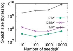
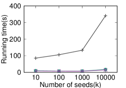
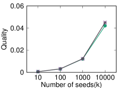
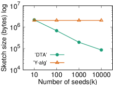
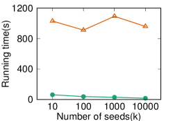
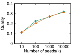
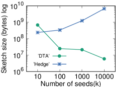
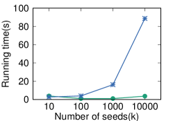
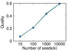
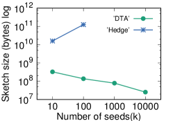
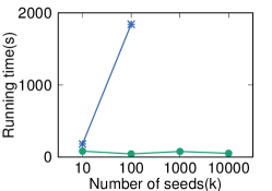
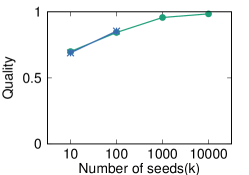
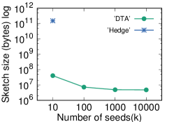
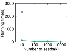
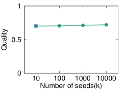
The experiment results are shown in Fig. 1. The proposed DTA is several orders of magnitude faster and using several orders less space, while providing comparable solution quality. For example, on Twitter, DTA uses 3735x less space and 19x faster for $k=10$. Hedge cannot complete within the time/space limit for other values of $k$.

6.3. Results on Influence Maximization

We compare DTA with IMM (Tang et al., 2015) and DSSA (Nguyen et al., 2016a) RIS-based algorithms that provide $(1-1/e-\epsilon)$ approximation guarantee.

The algorithms are compared on the popular independent cascade (IC) model (Kempe et al., 2003) and the probabilities on the edges are selected at random from $\{0.1,0.01,0.001\}$ following (Cohen et al., 2014; Chen et al., 2010; Jung et al., 2012). This settings of weights has been shown to be challenging in recent studies (Tang et al., 2017; Arora et al., 2017).

The results are shown in Fig. 2. Unfortunately, none of the two algorithms IMM (Tang et al., 2015) and DSSA (Nguyen et al., 2013) can complete within the time/space limit on Orkut and Twitter. Thus, only the results for DBLP are available.

On DBLP, DTA use 122x less space than IMM and 2.6x less space than DSSA. All algorithms produce solutions with similar quality. We note that on bigger network the reduction in space will be much larger. Unfortunately, none of the two algorithms can complete in the larger networks.

6.4. Results on Landmark Selection

For landmark selection, we compare DTA with Y-alg (Yoshida, 2014) state-of-the-art algorithm for Landmark selection (aka coverage centrality maximizations). Note that Y-alg only provide (arguably weaker) addictive theoretical guarantees (see Table 1).

The results are consistent with those in the previous applications. DTA uses 24 time less space and runs 59 times faster than Y-alg, while providing comparable solution quality.

Overall, our reduced sketch approach reduces the space up to several orders of magnitude while providing comparable running time and solution quality. The proposed algorithm DTA with adaptive sampling technique can further reduces the number of samples to provide $1-1/e-\epsilon$ approximation guarantee. Thus, DTA, with optimal approximation guarantee and optimal space complexity, and practical scalability provides an ideal solutions for $k$-cover and related applications.

7. Conclusion

We introduce a simple, space and time-efficient algorithmic framework, called BCA, that finds a near-optimal $(1-1/e-\epsilon)$-approximate solution for the fundamental $k$-cover problem. Our algorithms only requires $O(\epsilon^{-2}n\log n)$-space thanks to reduced sketch feature, $O(\epsilon^{-2}kn\log n)$-time and can be easily extended to budgeted, weighted versions. The empirical results show a leap performance benefit in saving time and memory in various applications of $k$-cover in comparison existing algorithms.

8. Concentration inequalities

We use the following concentration inequality.

Lemma 9.

Let $X^{(i)}_{S},i=1..N$ be $N$ Bernoulli random variables with the same mean $0\leq\mu_{S}\leq 1$ defined in Eq. (7). Then for any $x\geq 0$,

$$\Pr\Big{[}\max_{1\leq j\leq N}\big{|}\sum_{i=1}^{j} (X^{(i)}_{S}-\mu_{S})\big{|}\geq x\Big{]}\leq$$

$$2\exp\Big{(}\frac{-x^{2}}{2(N\mu_{S}(1-\mu_{S})+\frac{1}{3}x)}\Big{)}.$$

To prove the above concentration inequality, we use the following general Hoeffding’s bounds for supermartingales stated in Theorem 2.1 and Remark 2.1 of (Fan et al., 2012):

Lemma 10 ((Fan et al., 2012)).

Assume that $(\xi_{i},\mathcal{F}_{i})_{i=1,\dots,N}$ are supermartingale differences satisfying $\xi_{i}\leq 1$. Let $\Sigma_{j}=\sum_{i=1}^{j}\xi_{i}$. Then, for any $x\geq 0$ and $v>0$, the following bound holds,

$$\Pr\left[\Sigma_{j}\geq x\text{ and }\langle\Sigma\rangle_{j}\leq v^{2}\text{ for some }j=1,\dots,N\right]$$

(37) $$\leq\exp\Big{(}-\frac{x^{2}}{2(v^{2}+\frac{1}{3}x)}\Big{)},$$

where $\langle\Sigma\rangle_{j}=\sum_{i=1}^{j}\mathbb{E}(\xi_{i}^{2}|\mathcal{F}_{i-1})$.

By choosing $v^{2}=\sum_{i=1}^{N}\mathbb{E}(\xi_{i}^{2}|\mathcal{F}_{i-1})$, we have $\langle\Sigma\rangle_{j}\leq v^{2},\forall j=1,\dots,N$ and thus,

(38) $$\Pr\Big{[}\max_{1\leq j\leq n}\Sigma_{j}\geq x\Big{]}\leq\exp\Big{(}-\frac{x^{2}}{2(v^{2}+\frac{1}{3}x)}\Big{)}.$$

In our context of $k$-cover, based on random variables $X^{(j)}_{S}$ defined in Eq. (7), we define another set of random variables,

(39) $$\xi_{j}=X^{(j)}_{S}-\mu_{S},$$

that satisfy $-\mu_{S}\leq\xi_{j}\leq 1-\mu_{S}$ and form a sequence of supermartingale differences since

(40) $$\mathbb{E}[\xi_{j}|\mathcal{F}_{j-1}]=\mathbb{E}\left[X^{(j)}_{S}-\mu_{S}\right]=0,$$

where $\{\mathcal{F}_{i}\}_{i=1,2,\dots}$ is a filtration in which $\mathcal{F}_{i}$ is the $\sigma$-algebra defined on the outcomes of the first $i$ Bernoulli variables $\xi_{j},\forall j=1,\dots,i$. Thus, the inequality bound (38) simplifies in our case to,

$$\Pr\Big{[}\max_{1\leq j\leq N}\sum_{i=1}^{j} (X^{(i)}_{S}-\mu_{S})\geq x\Big{]}\leq$$

$$\exp\Big{(}-\frac{x^{2}}{2(N\mu_{S}(1-\mu_{S})+\frac{1}{3}x)}\Big{)}.$$

Similarly considering $\xi_{j}=\mu_{S}-X^{(j)}_{S}$, we obtain

$$\Pr\Big{[}\max_{1\leq j\leq N}\sum_{i=1}^{j} (X^{(i)}_{S}-\mu_{S})\leq-x\Big{]}\leq$$

$$\exp\Big{(}-\frac{x^{2}}{2(N\mu_{S}(1-\mu_{S})+\frac{1}{3}x)}\Big{)}.$$

From Lemma 9, we derive the number of random variables $X^{(j)}_{S}$ to provide the concentration bound with a fixed probability $\delta$.

Corollary 0.

Let $X^{(i)}_{S},i=1..N$ be $N$ Bernoulli random variables with mean $0\leq\mu_{S}\leq 1$ defined in Eq. (7). Let

(41) $$N(\epsilon,\delta,\mu)=2\Big{(}1+\frac{1}{3}\Big{)}\frac{1}{\mu\epsilon^{2}}\ln\Big{(}\frac{2}{\delta}\Big{)}.$$

Then for $\epsilon\geq 0$, $\mu\geq\mu_{S}$ and $N\geq N(\epsilon,\delta,\mu)$,

(42) $$\Pr\Big{[}\max_{1\leq j\leq N}\big{|}\sum_{i=1}^{j}(X^{(i)}_{S}-\mu_{S})\big{|}\geq\epsilon\mu N\Big{]}\leq\delta.$$

9. Omitted Proofs

First, we introduce some essential definitions used in our proof. Let $0<\alpha<1$ be a small constant, e.g. $\alpha=0.1$ and fixed $0<p<1$, e.g, $p=1/n$. Define

(43) $$\epsilon_{2} =\frac{\sqrt{\log p+\log\leavevmode\resizebox{14.22636pt}{}{${n\choose k}$}}}{(1-1/e)\sqrt{\log p}+\sqrt{\log p+\log\leavevmode\resizebox{14.22636pt}{}{${n\choose k}$}}}\frac{\epsilon}{1+\alpha},$$

(44) $$c =\frac{(1+\epsilon_{2})}{(1-\epsilon_{2})(1-1/e)},p=\frac{4(1+\left\lceil\log_{1+\alpha}c\right\rceil)}{\delta},$$

$$z^{*}=\frac{1+\epsilon_{2}}{1-1/e}\left(2+\frac{2}{3}\epsilon_{2}(1-\alpha)\right)\epsilon_{2}^{-2}\log\left(p{n\choose k}\right)$$

(45) $$=O\left(\epsilon^{-2}k\log n\right),$$

and,

(46) $$T^{*}=z^{*}\frac{(1-1/e)(1+\alpha)^{2}}{(1+\epsilon_{2})}\frac{1}{\textsf{OPT}}=O\left(\epsilon^{-2}k\log n\frac{1}{\textsf{OPT}}\right).$$

Proof of Lemma 6.

$\bullet$ Prove $T\geq T^{*}$ with probability $1-2/p$. Consider the case when $T^{*}$ hyperedges have been acquired. Apply the bound in Corollary 1 for a set $S$ with $\mu=\mu_{S^{*}}=\textsf{OPT}\geq\mu_{S}$ and note that $T^{*}\geq N(\epsilon_{2},\frac{1}{p{n\choose k}},\textsf{OPT})$,

(47) $$\Pr\Big{[}\max_{1\leq j\leq T^{*}}\big{|}\sum_{i=1}^{j}(X^{(i)}_{S}-\mu_{S})\big{|}\geq\epsilon_{2}\mu_{S^{*}}T^{*}\Big{]}\leq\frac{2}{p{n\choose k}}.$$

The inequality bound (47) is essential through the whole proof and reused multiple times later on. From (47), since there are at most ${n\choose k}$ sets having exactly $k$ nodes,

$$\Pr\Big{[}\max_{1\leq j\leq T^{*},|S|=k}\big{|}\sum_{i=1}^{j}(X^{(i)}_{S}-\mu_{S})\big{|}\geq\epsilon_{2}\mu_{S^{*}}T^{*}\Big{]}\leq\frac{2}{p}$$

$$\Rightarrow\text{ } \Pr\Big{[}\max_{1\leq j\leq T^{*},|S|=k}\sum_{i=1}^{j}X^{(i)}_{S}\geq\mu_{S}\cdot j+\epsilon_{2}\mu_{S^{*}}T^{*}\Big{]}\leq\frac{2}{p}.$$

Note that $\mu_{S}\leq\mu_{S^{*}}=\textsf{OPT},j\leq T^{*}$. Replacing $\mu_{S}$ by $\mu_{S^{*}}$, plugging $T^{*}$ and simplifying the above equation give

(48) $$\Pr\Big{[}\max_{1\leq j\leq T^{*},|S|=k}\sum_{i=1}^{j}X^{(i)}_{S}\geq(1-\frac{1}{e})z^{*}\Big{]}\leq\frac{2}{p}$$

In other words, with a probability of $1-\frac{2}{p}$, there is no set of $k$ nodes that can cover $(1-\frac{1}{e})z^{*}$ acquired hyperedges or more. However, since BCA returns a set that covers at least $(1-\frac{1}{e})z^{*}$ hyperedges (Lemma 3) when $z=z^{*}$. That means that BCA acquires more at least $T^{*}$ hyperedges with probability $1-2/p$.

$\bullet$ Prove $T<\frac{(1+\epsilon_{2})}{(1-\epsilon_{2})(1-1/e)}T^{*}$ with probability $1-2/p$. Similar to (47), for the optimal set $S^{*}$, we have with $T^{\prime}=\frac{(1+\epsilon_{2})}{(1-\epsilon_{2})(1-1/e)}T^{*}$

$$\Pr\Big{[}\max_{1\leq j\leq T^{\prime}}\big{|}\sum_{i=1}^{j}(X^{(i)}_{S^{*}}-\mu_{S^{*}})\big{|}\geq\epsilon_{2}\mu_{S^{*}}T^{\prime}\Big{]}\leq\frac{2}{p{n\choose k}}.$$

Consider the last $j=T^{\prime}$ and rearrange the terms, we get

$$\Pr\Big{[}\sum_{i=1}^{T^{\prime}}X^{(i)}_{S^{*}}\leq\mu_{S^{*}}\cdot T^{\prime}-\epsilon_{2}\mu_{S^{*}}T^{\prime}\Big{]}\leq\frac{2}{p{n\choose k}}.$$

Placing $T^{\prime}=\frac{(1+\epsilon_{2})}{(1-\epsilon_{2})(1-1/e)}T^{*}$ gives

$$\Pr\Big{[}\sum_{i=1}^{T^{\prime}}X^{(i)}_{S^{*}}\leq(1-\epsilon_{2})\mu_{S^{*}}\frac{(1+\epsilon_{2})}{(1-\epsilon_{2})(1-1/e)}T^{*}\Big{]}\leq\frac{2}{p{n\choose k}}$$

(49) $$\Rightarrow\text{ } \Pr\Big{[}\sum_{i=1}^{T^{\prime}}X^{(i)}_{S^{*}}\leq z^{*}\Big{]}\leq\frac{2}{p{n\choose k}}\leq\frac{2}{p}$$

Thus, with a probability of at least $1-\frac{2}{p},\sum_{i=1}^{T^{\prime}}X^{(i)}_{S^{*}}>z^{*}$ happens. However, BCA guarantees that the coverage of any set on the acquired hyperedges is at most $z^{*}$. That means $T<\frac{(1+\epsilon_{2})}{(1-\epsilon_{2})(1-1/e)}T^{*}$ with probability at least $1-2/p$. ∎

Proof of Lemma 7.

We prove the guarantee in each interval and then combine all the intervals to get the overall approximation guarantee.

$\bullet$ Consider an interval $[L_{i},U_{i}]$. Let define $\mathcal{B}_{S}$ the collection of bad sets of $k$ nodes in the sense that the coverage of each set is less than $(1-1/e-\epsilon)$ the optimal coverage of $k$ nodes, i.e. $\forall S\in\mathcal{B}_{S},\textbf{Cov}_{w}(S)<(1-1/e-\epsilon)\textsf{OPT}{}$ or similarly $\forall S\in\mathcal{B}_{S},\mu_{S}<(1-1/e-\epsilon)\mu_{S^{*}}$. We show that any bad set in $\mathcal{B}_{S}$ is returned with probability at most $\frac{4}{p}$ by considering two events:

• $\max_{L_{i}\leq j\leq U_{i}}\frac{\sum_{i=1}^{j}X^{(i)}_{S^{*}}}{j}\leq(1-\frac{\epsilon-\epsilon_{2}(1+\alpha)}{1-1/e})\mu_{S^{*}}$ and the returned solution $\hat{S}\in\mathcal{B}_{S}$.

• $\max_{L_{i}\leq j\leq U_{i}}\frac{\sum_{i=1}^{j}X^{(i)}_{S^{*}}}{j}>(1-\frac{\epsilon-\epsilon_{2}(1+\alpha)}{1-1/e})\mu_{S^{*}}$ and the returned solution $\hat{S}\in\mathcal{B}_{S}$.

Thus, the probability of returning a set $S\in\mathcal{B}_{S}$ is

$$\Pr[E1]+\Pr[E2].$$

We bound each of these events in the following.

The probability of the first joint event (E1) is less than the probability of $\max_{L_{i}\leq j\leq U_{i}}\frac{\sum_{i=1}^{j}X^{(i)}_{S^{*}}}{j}\leq(1-\frac{\epsilon-\epsilon_{2}}{1-1/e})\mu_{S^{*}}$ which is bounded by $\frac{2}{p}$ as shown below.

Apply Corollary 1 with $\mu=\mu_{S^{*}}=\textsf{OPT}$ and $N=U_{i}\geq T^{*}\geq N(\frac{\epsilon/(1+\alpha)-\epsilon_{2}}{1-1/e},\frac{1}{p},\mu_{S^{*}})$,

$$\Pr\Big{[}\max_{1\leq j\leq U_{i}}\Big{|}\sum_{i=1}^{j}(X^{(i)}_{S^{*}}-\mu_{S^{*}})\Big{|}\geq\frac{\epsilon/(1+\alpha)-\epsilon_{2}}{1-1/e}\mu_{S^{*}}U_{i}\Big{]}\leq\frac{2}{p}$$

Consider the sub-interval $j\in[L_{i},U_{i}]$ and note that $\frac{U_{i}}{j}\leq\frac{U_{i}}{L_{i}}=(1+\alpha)$ and rearrange the terms, we obtain:

$$\Pr[E1] =\Pr\Big{[}\max_{L_{i}\leq j\leq U_{i}}\frac{\sum_{i=1}^{j}X^{(i)}_{S^{*}}}{j}\leq(1-\frac{\epsilon-\epsilon_{2}(1+\alpha)}{1-1/e})\mu_{S^{*}}\Big{]}$$

$$\leq\frac{2}{p}.$$

The second joint event (E2) implies:

• $\sum_{i=1}^{T}X^{(i)}_{\hat{S}}\geq(1-1/e)\sum_{i=1}^{T}X^{(i)}_{S^{*}}$ (due to Lemma 3)

• $\mu_{\hat{S}}<(1-1/e-\epsilon)\mu_{S^{*}}$

• $\frac{\sum_{i=1}^{T}X^{(i)}_{S^{*}}}{T}>(1-\frac{\epsilon-\epsilon_{2}(1+\alpha)}{1-1/e})\mu_{S^{*}}$

From the three above inequalities, we derive

$$\frac{\sum_{i=1}^{T}X^{(i)}_{\hat{S}}}{T} \geq(1-1/e)\frac{\sum_{i=1}^{T}X^{(i)}_{S^{*}}}{T}$$

$$>(1-1/e)(1-\frac{\epsilon-\epsilon_{2}(1+\alpha)}{1-1/e})\mu_{S^{*}}$$

$$>(1-1/e-\epsilon)\mu_{S^{*}}+\epsilon_{2}(1+\alpha)\mu_{S^{*}}$$

(50) $$>\mu_{\hat{S}}+\epsilon_{2}(1+\alpha)\mu_{S^{*}}.$$

Hence, the probability of (E2) is bounded by

$$\Pr[E2]\leq\Pr\Big{[}\max_{L_{i}\leq j\leq U_{i}}\frac{\sum_{i=1}^{j}X^{(i)}_{\hat{S}}}{j}>\mu_{\hat{S}}+(1+\alpha)\epsilon_{2}\mu_{S^{*}}\Big{]}.$$

Apply again Corollary 1 on a set $S$ with $U_{i}\geq T^{*}\geq N((1+\alpha)\epsilon_{2},\frac{1}{p}\frac{1}{{n\choose k}},\mu_{S^{*}})$ hyperedges and consider the sub-interval $[L_{1},U_{1}]$,

$$\Pr\Big{[}\max_{L_{i}\leq j\leq U_{i}}\Big{|}\sum_{i=1}^{j}(X^{(i)}_{S}-\mu_{S})\Big{|}\geq(1+\alpha)\epsilon_{2}\mu_{S^{*}}U_{i}\Big{]}\leq\frac{2}{p}\frac{1}{{n\choose k}}$$

$$\Rightarrow\text{ }\Pr\Big{[}\max_{L_{i}\leq j\leq U_{i}}\frac{\sum_{i=1}^{j}X^{(i)}_{\hat{S}}}{j}-\mu_{\hat{S}}\geq\epsilon_{2}(1+\alpha)\mu_{S^{*}}\Big{]}\leq\frac{2}{p}.$$

Therefore, we obtain

(51) $$\Pr[E2]\leq\frac{2}{p}.$$

Combine the probabilities of (E1) and (E2), we find that the probability of returning a bad set is at most $\frac{4}{p}$ when $T\in[L_{i},U_{i}]$.

$\bullet$ Consider all $[L_{i},U_{i}]$, $\forall i=1,\dots,\left\lceil\log_{1+\alpha}c\right\rceil$. The probability of returning a bad set in any of the intervals $[L_{i},U_{i}]$ is bounded by

(52) $$\left\lceil\log_{1+\alpha}c\right\rceil\frac{4}{p},$$

because there are $\left\lceil\log_{1+\alpha}c\right\rceil$ such intervals. ∎

9.1. Proof of Lemma 8

We state the following general lemma and apply it in a straightforward manner to derive the results in Lemma 8.

Lemma 11.

Let $X_{1},X_{2},\dots,X_{N}$ be weakly dependent Bernoulli random variables satisfying $\forall i=1..N,$

$$E[X_{i}|X_{1},X_{2},\ldots,X_{i-1}]=E[X_{i}^{2}|X_{1},X_{2},\ldots,X_{i-1}]=\mu.$$

For $\delta\in(0,1)$, define $c_{i}=\ln(\frac{1}{\delta})/i,a=\frac{i}{N}$ and $\hat{\mu}_{i}=\frac{1}{j}\sum_{j=1}^{i}X_{j}$,

(53) $$\Pr\left[\mu\geq f_{L}(i,\hat{\mu}_{i},\delta,N),\ \forall i=1..N\right]\geq 1-\delta,$$

(54) $$\Pr\left[\mu\leq f_{U}(i,\hat{\mu}_{i},\delta,N),\ \forall i=1..N\right]\geq 1-\delta,$$

where

(55) $$f_{L}(i,\hat{\mu}_{i},\delta,N)=\min\Bigg{\{}\hat{\mu}_{i}+\frac{(\hat{\mu}_{i}-1)c_{i}}{3-c_{i}},$$

$$\leavevmode\resizebox{227.62204pt}{}{$\frac{3c_{i}+3a\hat{\mu}_{i}-ac_{i}(\hat{\mu}_{i}+1)-\sqrt{c_{i}^{2}(3+a(\hat{\mu}_{i}-1))^{2}+18a(1-\hat{\mu}_{i})\hat{\mu}_{i}}}{c_{i}(6-2a)+3a}$}\Bigg{\}},$$

and,

(56) $$f_{U}(i,\hat{\mu}_{i},\delta,N)=\max\Bigg{\{}\hat{\mu}_{i}+\frac{(i-\hat{\mu}_{i})c_{i}}{3+c_{i}},$$

$$\leavevmode\resizebox{227.62204pt}{}{$\frac{3c_{i}+3a\hat{\mu}_{i}+ac_{i}(1+\hat{\mu}_{i})+\sqrt{c_{i}^{2}(3+a(1-\hat{\mu}_{i}))^{2}+18a(1-\hat{\mu}_{i})\hat{\mu}_{i}}}{c_{i}(6+2a)+3a}$}\Bigg{\}}.$$

From the bound in Lemma 9, we derive the following:

Lemma 0.

Given Bernouli random variables $X_{1},\ldots,X_{N}$ with mean $E[X_{i}]=\mu\leq 1/2$, let $\hat{\mu}_{i}=\frac{1}{i}\sum_{j=1}^{i}X_{j}$, $\delta\in(0,1)$ and fixed $N$. Denote $c=\ln(\frac{1}{\delta})/N$ and $t=\frac{1}{3}c(1-\mu)+\sqrt{\frac{1}{9}c^{2}(1-\mu)^{2}+2\mu(1-\mu)c}$,

(57) $$\Pr\left[\hat{\mu}_{i}-\mu\leq\frac{N}{i}t,\ \forall i=1..N\right]\geq 1-\delta,$$

and,

(58) $$\Pr\left[\hat{\mu}_{i}-\mu\geq-\frac{N}{i}t,\ \forall i=1..N\right]\geq 1-\delta.$$

Proof.

Deriveing Lower-bound function: By Lemma 1, we have

(59) $$\Pr\left[\hat{\mu}_{i}-\mu\leq\frac{N}{i}t,\ \forall i=1..N\right]\geq 1-\delta,$$

where

(60) $$t=\frac{1}{3}c(1-\mu)+\sqrt{\frac{1}{9}c^{2}(1-\mu)^{2}+2\mu(1-\mu)c}.$$

Therefore, with probability at least $1-\delta$, $\forall i=1..N$

$$\hat{\mu}_{i}-\mu\leq\frac{1}{3}c_{i}(1-\mu)+\sqrt{\frac{c_{i}^{2}}{9}(1-\mu)^{2}+2\mu(1-\mu)c_{i}\frac{N}{i}}$$

$$\Leftrightarrow\text{ } \hat{\mu}_{i}-\mu-\frac{1}{3}c_{i}(1-\mu)\leq\sqrt{\frac{c_{i}^{2}}{9}(1-\mu)^{2}+2\mu(1-\mu)c_{i}\frac{N}{i}}$$

From the above inequality, $\forall i=1..N$, consider two cases:

• $\hat{\mu}_{i}-\mu-\frac{1}{3}c_{i}(1-\mu)<0$, then $\mu>\frac{\hat{\mu}_{i}-c_{i}/3}{1-c_{i}/3}$

• $\hat{\mu}_{i}-\mu-\frac{1}{3}c_{i}(1-\mu)\geq 0$, then taking the square of two sides, we have,

  (61) $$\left(\hat{\mu}_{i}-\mu-\frac{c_{i}}{3}(1-\mu)\right)^{2}\leq\frac{c_{i}^{2}}{9}(1-\mu)^{2}+2c_{i}\frac{N}{i}\mu(1-\mu).$$

  Solve the above quadratic inequality for $\mu$, we obtain another lower-bound for $\mu$.

Deriving Upper-bound function. By Lemma 1,

(62) $$\Pr\left[\hat{\mu}_{i}-\mu\geq-\frac{n}{i}t,\ \forall i=1..N\right]\geq 1-\delta.$$

Follow the similar steps as in deriving the lower-bound function above, we obtain the upper-bound function in the lemma. ∎

The lower-bound function $f_{L}(N_{j},d_{c}/N_{j},\delta^{\prime},N_{j})$ is directly obtained from $f_{L}(i,\hat{\mu}_{i},\delta,N)$. Notice that we can replace $\hat{\mu}_{i}$ in the upper-bound $f_{U}(i,\hat{\mu}_{i},\delta,N)$ by a larger number and still obtain an upper-bound with the same probability guarantee. Thus, the upper-bound $f_{U}\big{(}T_{z},z/T_{z},\delta^{\prime},\left\lceil(1+\beta)^{t_{u}}\right\rceil\big{)}$ is derived from $f_{U}(i,\hat{\mu}_{i},\delta,N)$ by using the larger value $z/T$ for the coverage of optimal solution.

9.2. Proof of Theorem 1

DTA returns either $S_{z}$ when the test $\rho_{S}\geq 1-1/e-\epsilon$ succeeds (Lines 9, 10) or $S_{z^{*}}$ (Line 13). We show that the corresponding returned solutions are $(1-1/e-\epsilon)$-approximate with probabilities $1-4\delta/3$ and $1-\delta$, respectively. Then the lemma follows by adding these probabilities.

Return $S_{z}$ when the test $\rho_{S}\geq 1-1/e-\epsilon$ succeeds. The $(1-1/e-\epsilon)$ approximation ratio is directly obtained by Lemma 8. The probability of this guarantee is computed by taking the sum of the two probabilities in Lemma 8 times the number of times that $\rho_{S}$ is computed. By Lemma 8, each bound $\rho_{S}$ holds with prob. $1-2\delta^{\prime}=1-\frac{\delta}{\log_{2}(z^{*})\log_{1+\beta}(cT^{*})}$ since the lower and upper bounds returned by $f_{L}(.)$ and $f_{U}(.)$ individually hold with probability $1-\delta^{\prime}$. We show that the total number of times that $f_{L}(.)$ and $f_{U}(.)$ are computed is at most $\log_{2}(z^{*})\log_{1+\beta}(cT^{*})$ with probability $1-\delta/3$. Then, the accumulated probability is given by $1-\frac{\delta}{\log_{2}(z^{*})\log_{1+\beta}(cT^{*})}\cdot\log_{2}(z^{*})\log_{1+\beta}(cT^{*})-\delta/3=1-4\delta/3$. Thus, it is sufficient to show that the total number of times that $f_{L}(.)$ and $f_{U}(.)$ are computed is at most $\log_{2}(z^{*})\log_{1+\beta}(cT^{*})$.

For $z=z^{*}/2^{i},i\geq 1$, similar to the proof of Eq. (49), BCA with threshold $z$ acquires $T\geq cT^{*}$ hyperedges with probability at most

(63) $$\Pr\Big{[}\sum_{i=1}^{T}X^{(i)}_{S^{*}}\leq z\Big{]}\leq 2\Big{(}\frac{1}{p}\Big{)}^{2^{i}}<2\Big{(}\frac{1}{p}\Big{)}^{i}.$$

Thus, the probability that BCA with $z$ samples at most $cT^{*}$ hyperedges, hence, there are at most $\log_{1+\beta}(cT^{*})$ times that $f_{L}(.)$ and $f_{U}(.)$ are computed, is $1-2(\frac{1}{p})^{i}$. Then, accumulating this probability over all BCA calls with $z\in\Big{\{}\frac{z^{*}}{2^{i_{0}}},\frac{z^{*}}{2^{i_{0}-1}},\dots,z^{*}\Big{\}}$, we obtain the probability of DTA having at most $\log_{2}(z^{*})\log_{1+\beta}(cT^{*})$ computation rounds of $f_{L}(.)$ and $f_{U}(.)$ to be at least

(64) $$1-\sum_{i=1}^{\log_{2}(z^{*})}2\Big{(}\frac{1}{p}\Big{)}^{i}\geq 1-2\frac{1}{p}\frac{1}{1-1/p}\geq 1-\frac{\delta}{3},$$

where $p$ was replaced by its definition in Eq. (24).

DTA returns $S_{z^{*}}$. By Theorem 1, BCA with $z=z^{*}$ finds an $(1-1/e-\epsilon)$-approximate solution with probability $1-\delta$.

References

- (1)
- sna (2017) 07.01.2017. Stanford network analysis project. http://snap.stanford.edu..
- Arora et al. (2017) A. Arora, S. Galhotra, and S. Ranu. 2017. Debunking the myths of influence maximization: An in-depth benchmarking study. In SIGMOD. 651–666.
- Bateni et al. (2018) M. Bateni, H. Esfandiari, and V. Mirrokni. 2018. Optimal Distributed Submodular Optimization via Sketching. In SIGKDD. 1138–1147.
- Borgs et al. (2014) C. Borgs, M. Brautbar, J. Chayes, and B. Lucier. 2014. Maximizing Social Influence in Nearly Optimal Time. In SODA. SIAM, 946–957.
- Borgwardt (1987) K. Borgwardt. 1987. The Simplex Algorithm: A Probabilistic Analysis, Algorithms and Combinatorics.
- Chen et al. (2010) W. Chen, Y. Yuan, and L. Zhang. 2010. Scalable influence maximization in social networks under the linear threshold model. In ICDM. 88–97.
- Cohen et al. (2014) E. Cohen, D. Delling, T. Pajor, and R. F. Werneck. 2014. Sketch-based influence maximization and computation: Scaling up with guarantees. In CIKM. 629–638.
- Dagum et al. (2000) P. Dagum, R. Karp, M. Luby, and S. Ross. 2000. An Optimal Algorithm for Monte Carlo Estimation. SICOMP (2000), 1484–1496.
- Domingos and Richardson (2001) P. Domingos and M. Richardson. 2001. Mining the network value of customers. In KDD. ACM, 57–66.
- Du et al. (2013) N. Du, L. Song, M. Gomez-Rodriguez, and H. Zha. 2013. Scalable influence estimation in continuous-time diffusion networks. In NIPS. 3147–3155.
- Fan et al. (2012) X. Fan, I. Grama, and Q. Liu. 2012. Hoeffding’s inequality for supermartingales. Stochastic Processes and their Applications 122, 10 (2012), 3545–3559.
- Feige (1998) U. Feige. 1998. A threshold of ln n for approximating set cover. JACM (1998), 634–652.
- Huang et al. (2017) K. Huang, S. Wang, G. Bevilacqua, X. Xiao, and L. V. S. Lakshmanan. 2017. Revisiting the stop-and-stare algorithms for influence maximization. VLDB (2017), 913–924.
- Jung et al. (2012) K. Jung, W. Heo, and W. Chen. 2012. Irie: Scalable and robust influence maximization in social networks. In ICDM. 918–923.
- Karp (1972) R. M. Karp. 1972. Reducibility among combinatorial problems. In Complexity of computer computations. Springer, 85–103.
- Kempe et al. (2003) D. Kempe, J. Kleinberg, and É. Tardos. 2003. Maximizing the spread of influence through a social network. In KDD. 137–146.
- Kwak et al. (2010) H. Kwak, C. Lee, H. Park, and S. Moon. 2010. What is Twitter, a social network or a news media?. In WWW. 591–600.
- Leskovec et al. (2007) J. Leskovec, A. Krause, C. Guestrin, C. Faloutsos, J. VanBriesen, and N. Glance. 2007. Cost-effective outbreak detection in networks. In KDD. 420–429.
- Mahmoody et al. (2016) A. Mahmoody, C. E. Tsourakakis, and E. Upfal. 2016. Scalable Betweenness Centrality Maximization via Sampling. In KDD. 1765–1773.
- McGregor and Vu (2017) A. McGregor and H. T. Vu. 2017. Better Streaming Algorithms for the Maximum Coverage Problem. In ICDT. 1–18.
- Megiddo (1984) N. Megiddo. 1984. Linear programming in linear time when the dimension is fixed. JACM 31, 1 (1984), 114–127.
- Nemhauser and Wolsey (1981) G. L. Nemhauser and L. A. Wolsey. 1981. Maximizing submodular set functions: formulations and analysis of algorithms. North-Holland Mathematics Studies (1981), 279–301.
- Nguyen et al. (2017) H. T. Nguyen, T. P. Nguyen, T. N. Vu, and T. N. Dinh. 2017. Outward Influence and Cascade Size Estimation in Billion-scale Networks. In SIGMETRICS. 63–63.
- Nguyen et al. (2013) H. T. Nguyen, M. T. Thai, and T. N. Dinh. 2013. Cost-aware Targeted Viral Marketing in Billion-scale Networks. In INFOCOM. 55–59.
- Nguyen et al. (2016a) H. T. Nguyen, M. T. Thai, and T. N. Dinh. 2016a. Stop-and-Stare: Optimal Sampling Algorithms for Viral Marketing in Billion-scale Networks. In SIGMOD. 695–710.
- Nguyen et al. (2016b) H. T. Nguyen, M. T. Thai, and T. N. Dinh. 2016b. Stop-and-Stare: Optimal Sampling Algorithms for Viral Marketing in Billion-scale Networks. arXiv preprint arXiv:1605.07990 (2016).
- Ohsaka et al. (2016) N. Ohsaka, T. Akiba, Y. Yoshida, and K. Kawarabayashi. 2016. Dynamic influence analysis in evolving networks. VLDB (2016), 1077–1088.
- Potamias et al. (2009) M Potamias, F. Bonchi, C. Castillo, and A. Gionis. 2009. Fast shortest path distance estimation in large networks. In CIKM. 867–876.
- Tang et al. (2018) J. Tang, X. Tang, X. Xiao, and J. Yuan. 2018. Online Processing Algorithms for Influence Maximization. In In SIGMOD. ACM, New York, NY, USA, 991–1005. https://doi.org/10.1145/3183713.3183749
- Tang et al. (2017) J. Tang, X. Tang, and J. Yuan. 2017. Influence Maximization Meets Efficiency and Effectiveness: A Hop-Based Approach. ASONAM (2017).
- Tang et al. (2015) Y. Tang, Y. Shi, and X. Xiao. 2015. Influence Maximization in Near-Linear Time: A Martingale Approach. In SIGMOD. 1539–1554.
- Tang et al. (2014) Y. Tang, X. Xiao, and Y. Shi. 2014. Influence maximization: Near-optimal time complexity meets practical efficiency. In SIGMOD. 75–86.
- Yoshida (2014) Y. Yoshida. 2014. Almost linear-time algorithms for adaptive betweenness centrality using hypergraph sketches. In KDD. 1416–1425.