Predictive Scotogenic Model with Flavor Dependent Symmetry

Abstract

In this paper, we propose a viable approach to realise two texture-zeros in the scotogenic model with flavor dependent $U(1)_{B-2L_{\alpha}-L_{\beta}}$ gauge symmetry. These models are extended by two right-handed singlets $N_{Ri}$ and two inert scalar doublets $\eta_{i}$, which are odd under the dark $Z_{2}$ symmetry. Among all the six constructed textures, texture $A_{1}$ and $A_{2}$ are the only two allowed by current experimental limits. Then choosing texture $A_{1}$ derived from $U(1)_{B-2L_{e}-L_{\tau}}$, we perform a detail analysis on the corresponding phenomenology such as predictions of neutrino mixing parameters, lepton flavor violation, dark matter and collider signatures. One distinct nature of such model is that the structure of Yukawa coupling $\bar{L}\tilde{\eta}N_{R}$ is fixed by neutrino oscillation data, and can be further tested by measuring the branching ratios of charged scalars $\eta_{1,2}^{\pm}$.

I Introduction

It is well known that the Standard Model (SM) needs extensions to accommodate two missing spices: the tiny but no-zero neutrino masses and the cosmological dark matter (DM) candidates. One way of incorporating above two issues in a unified framework is the scotogenic model Ma:2006km ; Krauss:2002px ; Aoki:2008av , where neutrinos are radiatively generated and the DM fields serves as intermediate messengers propagating inside the loop diagram. With all new particles around TeV scale, the scotogenic model leads to testable phenomenologies Ma:2006fn ; Hambye:2006zn ; Sierra:2008wj ; Suematsu:2009ww ; Schmidt:2012yg ; Bouchand:2012dx ; Ma:2012ez ; Klasen:2013jpa ; Ho:2013hia ; Modak:2014vva ; Molinaro:2014lfa ; Faisel:2014gda ; Merle:2015gea ; Ahriche:2016cio ; Lindner:2016kqk ; Hessler:2016kwm ; Borah:2017dfn ; Abada:2018zra ; Hugle:2018qbw ; Baumholzer:2018sfb ; Borah:2018rca ; Bian:2018bxr . Therefore, viable models are extensively studies in recent years Cai:2017jrq .

On the other hand, the understanding of the leptonic flavor structure is still one of the major open questions in particle physics. The consensus is that the leptonic mass texture is tightly restricted under the present experimental data. An attractive approach is to consider two texture-zeros in neutrino mass matrix ($M_{\nu}$) so that the number of parameters in the Lagrangian is reducedFrampton:2002yf . The phenomenological analysis of two texture-zeros models have been studied in Ref.Fritzsch:2011qv ; Alcaide:2018vni . Among fifteen logically patterns, seven of them are compatible to the low-energy experimental data.

On the theoretical side, the simplest way of realizing texture-zeros is to impose the discrete $Z_{N}$ flavor symmetryGrimus:2004hf . However, it might be more appealing to adopt gauge symmetries instead of discrete ones, because the latter may be treated as the residual of $U(1)$ gauge symmetry. It is noted that one can not set any restriction on lepton mass matrix by means of fields with flavor universal charges. Thus the flavor dependent $U(1)$ gauge symmetry is the reasonable choice. Along this thought of idea, specific models are considered in the context of seesaw mechanisms. In Ref.Araki:2012ip , the two texture-zeros are realized based on the anomaly-free $U(1)_{X}$ gauge symmetry with $X\equiv B-\sum x_{\alpha}L_{\alpha}(\alpha=e,\mu,\tau)$ being the linear combination of baryon number $B$ and the lepton numbers $L_{\alpha}$ per family. In Ref.Cebola:2013hta , more solutions are found in the type-I and/or III seesaw framework.

It is then natural to ask if predictive texture-zeros in $M_{\nu}$ can be realized in the scotogenic scenario and several attempts have been made in this direction. For example, one texture-zero is recently considered in Ref. Kitabayashi:2018bye . Texture $B_{1}$-$B_{4}$ have been discussed in a model-independent way in Ref. Kitabayashi:2017sjz . Texture $C$ is obtained by introducing $U(1)_{L_{\mu}-L_{\tau}}$ gauge symmetry Baek:2015mna ; Baek:2015fea ; Lee:2017ekw ; Asai:2018ocx . Texture $B_{2}$ is realised with $U(1)_{L_{e}+L_{\mu}-L_{\tau}}$ gauge symmetry in Ref. Nomura:2017ohi . If the quark flavor is also flavor dependent, e.g., $U(1)_{xB_{3}-xL_{e}-L_{\mu}+L_{\tau}}$, then one can further interpret the $R_{K}$ anomaly with texture $A_{1}$ Ko:2017quv . Other viable two texture-zeros are systematically realised in Ref. Nomura:2018rvy by considering the $U(1)_{B-2L_{\alpha}-L_{\beta}}$ gauge symmetry with three right-handed singlets. In this paper, we provide another viable approach. Under same flavor dependent $U(1)_{B-2L_{\alpha}-L_{\beta}}$ gauge symmetry, we introduce only two right-handed singlets but two inert scalars, leading to different texture-zeros. In aspect of predicted phenomenology, the texture $B_{1}$ considered in Ref. Nomura:2018rvy is marginally allowed by current Planck result for $\sum m_{i}<0.12$ eV Aghanim:2018eyx , we thus consider texture $A_{1}$ with latest neutrino oscillation data Esteban:2018azc as the benchmark model. In this case, the gauge symmetry is $U(1)_{B-2L_{e}-L_{\tau}}$ in our approach.

The rest of this paper is organised as follows. Start with classic scotogenic model in Sec. II, we first discuss the realization of texture-zeros in scotogenic model with $U(1)_{B-2L_{\alpha}-L_{\beta}}$ gauge symmetry in a general approach. Then the texture $A_{1}$ derived from $U(1)_{B-2L_{e}-L_{\tau}}$ is explained in detail. The corresponding phenomenological predictions, such as neutrino mixing parameters, lepton flavor violation rate, dark matter and highlights of collider signatures are presented in Sec. III. Finally, conclusions are summarised in Sec. IV.

II The Model Setup

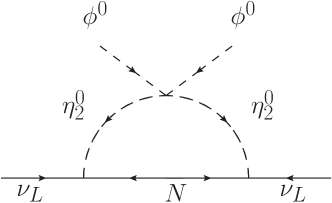
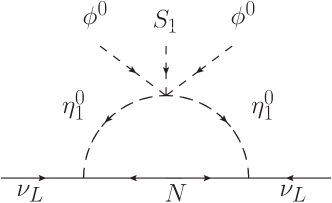
Figure 1: Radiative neutrino mass at one-loop. Left pattern is for classic scotogenic model, while right pattern is the additional contribution in our models.

II.1 Classic scotogenic model

In the classic scotogenic model proposed by Ma Ma:2006km , three right-handed fermion singlets $N_{Ri}(i=1\sim 3)$ and an inert scalar doublet field $\eta=(\eta^{+},\eta^{0})$ are added to the SM. In addition, a discrete $Z_{2}$ symmetry is imposed for the new fields in order to forbid the tree-level neutrino Yukawa interaction and stabilize the DM candidate. The relevant interactions for neutrino masses generation are given by

$$\mathcal{L}~{}\supset~{}h_{\alpha i}\overline{L}_{\alpha}\tilde{\eta}N_{Ri}+\frac{1}{2}M_{N}\overline{N}_{R}^{c}N_{R}+\frac{1}{2}\lambda(\Phi^{\dagger}\eta)^{2}+\text{h.c.}.$$ (1)

The mass matrix $M_{N}$ can be diagonalized by an unitary matrix $V$ satisfying

$$V^{T}M_{N}V=\hat{M}_{N}\equiv\text{diag}(M_{N1},M_{N2},M_{N3}).$$ (2)

Due to the $Z_{2}$ symmetry, the neutrino masses are generated at one-loop level, as show in left pattern of Fig. 1. The neutrino mass matrix can be computed exactly, i.e.

$$(M_{\nu})_{\alpha\beta}=\frac{1}{32\pi^{2}}\sum_{k}h_{\alpha i}V_{ik}h_{\beta j}V_{jk}M_{Nk}\Big{[}\frac{m_{R}^{2}}{m_{R}^{2}\!-M_{Nk}^{2}}\log\big{(}\frac{m_{R}^{2}}{M_{Nk}^{2}}\big{)}-\frac{m_{I}^{2}}{m_{I}^{2}\!-M_{Nk}^{2}}\log\big{(}\frac{m_{I}^{2}}{M_{Nk}^{2}}\big{)}\Big{]}\\$$ (3)

where $m_{R}$ and $m_{I}$ are the masses of $\sqrt{2}\Re\eta^{0}$ and $\sqrt{2}\Im\eta^{0}$. If we assume $m_{0}^{2}\equiv(m_{R}^{2}+m_{I}^{2})/2\gg M_{Nk}^{2}$, $M_{\nu}$ are then given by

$$\begin{split}(M_{\nu})_{\alpha\beta}&\simeq-\frac{1}{32\pi^{2}}\frac{\lambda v^{2}}{m_{0}^{2}}\sum_{k}h_{\alpha i}V_{ik}h_{\beta j}V_{jk}M_{Nk}\\ &=-\frac{1}{32\pi^{2}}\frac{\lambda v^{2}}{m_{0}^{2}}(hM_{N}h^{T})_{\alpha\beta}\end{split}$$ (4)

The neutrino mass matrix $M_{\nu}$ is diagonalized as

$$U_{\text{PMNS}}^{T}M_{\nu}U_{\text{PMNS}}=\hat{m}_{\nu}\equiv\text{diag}(m_{1},m_{2},m_{3}),$$ (5)

where $U_{\text{PMNS}}$ is the neutrino mixing matrix denoted as

$$U_{\text{PMNS}}\!=\!\left(\begin{array}[]{ccc}c_{12}c_{13}&s_{12}c_{13}&s_{13}\\ -c_{12}s_{23}s_{13}-s_{12}c_{23}e^{-i\delta}&-s_{12}s_{23}s_{13}+c_{12}c_{23}e^{-i\delta}&s_{23}c_{13}\\ -c_{12}c_{23}s_{13}+s_{12}s_{23}e^{-i\delta}&-s_{12}c_{23}s_{13}-c_{12}s_{23}e^{-i\delta}&c_{23}c_{13}\end{array}\right)\!\times\!\text{diag}(e^{i\rho},e^{i\sigma},1)$$ (9)

Here, we define $c_{ij}=\cos\theta_{ij}$ and $s_{ij}=\sin\theta_{ij}$ ($ij=12,23,13$) for short, $\delta$ is the Dirac phase and $\rho,\sigma$ are the two Majorana phases as in Ref. Fritzsch:2011qv .

Group	Lepton Fields								Scalar Fields
	$L_{\alpha}$	$\ell_{\alpha R}$	$L_{\beta}$	$\ell_{\beta R}$	$L_{\gamma}$	$\ell_{\gamma R}$	$N_{R1}$	$N_{R2}$	$\Phi$	$\eta_{1}$	$\eta_{2}$	$S_{1}$	$S_{2}$
$SU(2)_{L}$	$2$	$1$	$2$	$1$	$2$	$1$	$0$	$0$	$2$	$2$	$2$	$1$	$1$
$U(1)_{Y}$	$-\frac{1}{2}$	$-1$	$-\frac{1}{2}$	$-1$	$-\frac{1}{2}$	$-1$	$1$	$1$	$\frac{1}{2}$	$\frac{1}{2}$	$\frac{1}{2}$	$0$	$0$
$Z_{2}$	$+$	$+$	$+$	$+$	$+$	$+$	$-$	$-$	$+$	$-$	$-$	$+$	$+$
$U(1)_{B-2L_{\alpha}-L_{\beta}}$	$-2$	$-2$	$-1$	$-1$	$0$	$0$	$-1$	$-2$	$0$	$-1$	$0$	$2$	$3$

Table 1: Particle content and corresponding charge assignments.

II.2 Two texture-zeros in scotogenic model

In this section, we demonstrate a class of scotogenic models with $G_{SM}\times U(1)_{B-2L_{\alpha}-L_{\beta}}\times Z_{2}$ gauge symmetry where two texture-zero structures in $M_{\nu}$ are successfully realized. The particle content and corresponding charge assignments are listed in Tab. 1. In the fermion sector, we introduce two right-handed $SU(2)_{L}$ singlets $N_{R1}$ and $N_{R2}$ and assume they carry the same no-zero $B-2L_{\alpha}-L_{\beta}$ charges as two of SM leptons respectively. Noticeably, if one further introduce one additional $N_{R3}$ with zero $B-2L_{\alpha}-L_{\beta}$ charge, the approach considered in Ref. Nomura:2018rvy are then reproduced. In terms of gauged $U(1)_{B-2L_{\alpha}-L_{\beta}}$ symmetry, the anomaly free conditions should be considered first and we find all anomalies are zero because

$$[SU(3)_{c}]^{2}U(1)_{X} : 3\times\frac{1}{2}\Big{(}\frac{2}{3}-\frac{1}{3}-\frac{1}{3}\Big{)}=0$$ (10)

$$U(1)_{Y}[U(1)_{X}]^{2} : 3\Big{[}6\Big{(}\frac{1}{6}\Big{)}\!-3\Big{(}\frac{2}{3}\Big{)}\!-3\Big{(}\frac{1}{3}\Big{)}\Big{]}\Big{(}\frac{1}{3}\Big{)}^{2}\!\!+\Big{[}2\Big{(}\!-\frac{1}{2}\Big{)}\!-\!\Big{(}\!-1\Big{)}\Big{]}\Big{[}(-1)^{2}+(-2)^{2}\Big{]}=0$$

$$[SU(2)_{L}]^{2}U(1)_{X} : \frac{1}{2}\Big{[}3\times 3\Big{(}\frac{1}{3}\Big{)}+(-1)+(-2)\Big{]}=0$$

$$[U(1)_{Y}]^{2}U(1)_{X} : 3\Big{[}6\Big{(}\frac{1}{6}\Big{)}^{2}-3\Big{(}\frac{2}{3}\Big{)}^{2}-3\Big{(}\frac{1}{3}\Big{)}^{2}\Big{]}\Big{(}\frac{1}{3}\Big{)}+\Big{[}2\Big{(}-\frac{1}{2}\Big{)}^{2}-\Big{(}-1\Big{)}^{2}\Big{]}(-1-2)=0$$

$$U(1)_{X}^{3} : 2(-1)^{3}-2(-1)^{3}+2(-2)^{3}-2(-2)^{3}=0$$

$$[\text{Gravity}]^{2}U(1)_{X} : 2(-1)-2(-1)+2(-2)-2(-2)=0$$

Let us now discuss the scotogenic realizations of two texture-zeros in $M_{\nu}$. With two $N_{R}$ components, $h$ and $M_{N}$ are $3\times 2$ and $2\times 2$ matrices respectively. From Eq.(4), it is clear that the texture-zeros of $M_{\nu}$ can be attributed to the texture-zeros in $h$ and $M_{N}$ matrices. In the original scotogenic model with an inert scalar doublet $\eta$ and two $N_{R}$ fields, the charge assignments for $U(1)_{B-2L_{\alpha}-L_{\beta}}$ gauge symmetry give rise to only two Yukawa terms for $h_{\alpha i}\overline{L}_{\alpha}\tilde{\eta}N_{Ri}(\alpha=e,\mu,\tau,i=1,2)$. In this case, at least two texture-zeros are placed in the same line of $h$ matrix, being therefore excluded experimentally. In order to accommodate the realistic neutrino mixing data, the scotogenic model are extended where, in scalar sector, two inert doublet $\eta_{1}$ and $\eta_{2}$ are introduced (see Tab. 1). In addition, two scalar singlet $S_{1}$ and $S_{2}$ are added so that $U(1)_{B-2L_{\alpha}-L_{\beta}}$ symmetry is spontaneously breaking after $S_{1,2}$ get the vacuum expectation value (VEV) $\langle S_{1,2}\rangle=v_{1,2}/\sqrt{2}$. Note that $N_{Ri}$ and $\eta_{i}$ are odd under the discrete $Z_{2}$ symmetry. Since we have two inert scalars, the relevant scalar interactions for the loop-induced neutrino masses is given by

$$\mathcal{L}_{S}~{}\supset\frac{\lambda}{\Lambda}(\Phi\eta_{1})^{2}S_{1}+\lambda^{\prime}(\Phi\eta_{2})^{2}+\text{h.c.},$$ (11)

where $\Lambda$ is a new high energy scale and the first term is a dimension-five operator guaranteed by the accidental $U(1)_{B-2L_{\alpha}-L_{\beta}}$ symmetry. One can achieve the effective operator by simply adding a new scalar singlet $\rho\sim(1,0,1,-)$ so that in scalar sector $\mathcal{L}_{S}~{}\supset\mu(\Phi^{\dagger}\eta)\rho^{\dagger}+\mu^{\prime}\rho^{2}S_{1}$ is allowed. Then the effective interaction $\lambda(\Phi\eta_{1})^{2}S_{1}/\Lambda$ is obtained by integrate the $\rho$ field out of $\mathcal{L}_{S}$ sector. In the following analysis, we adopt the expression of effective operator in Eq.(11) and do not consider its specific realization in detail.

The neutrinos acquire their tiny masses radiatively though the one-loop diagram depicted in Fig. 1. Therefore, the neutrino mass matrix is formulated by two different contribution, namely,

$$(M_{\nu})\propto hM_{N}h^{T}+fM_{N}f^{T},$$ (12)

where $h$ and $f$ are the Yukawa coupling texture for $\overline{L}_{\alpha}\tilde{\eta}_{1}N_{Ri}$ and $\overline{L}_{\alpha}\tilde{\eta}_{2}N_{Ri}$ with further assumption $\Lambda=\langle S_{1}\rangle$ and $\lambda=\lambda^{\prime}$. As a case study, we consider the $U(1)_{B-2L_{e}-L_{\tau}}$ gauge symmetry under which the flavor dependent Yukawa interaction is given by

$$-\mathcal{L}_{\text{Y}} = h_{\mu 1}\bar{L}_{\mu}\tilde{\eta}_{1}N_{R1}+h_{\tau 2}\bar{L}_{\tau}\tilde{\eta}_{1}N_{R2}+f_{\tau 1}\bar{L}_{\tau}\tilde{\eta}_{2}N_{R1}+f_{e2}\bar{L}_{e}\tilde{\eta}_{2}N_{R2}$$

$$+y_{11}\overline{N^{c}_{R1}}N_{R1}S_{1}+y_{12}(\overline{N^{c}_{R1}}N_{R2}+\overline{N^{c}_{R2}}N_{R1})S_{2}+\text{h.c.},$$

where from the charge assignment, the texture of fermion Yukawa coupling are

$$h=\left(\begin{array}[]{cc}0&0\\ h_{\mu 1}&0\\ 0&h_{\tau 2}\end{array}\right),\quad f=\left(\begin{array}[]{cc}0&f_{e2}\\ 0&0\\ f_{\tau 1}&0\end{array}\right),\quad y=\left(\begin{array}[]{cc}y_{11}&y_{12}\\ y_{12}&0\end{array}\right).$$ (22)

Texture of $M_{\nu}$	Group	Texture of $M_{\nu}$	Group	Status
$A_{1}:\left(\begin{array}[]{ccc}0&0&\times\\ 0&\times&\times\\ \times&\times&\times\end{array}\right)$	$U(1)_{B-2L_{e}-L_{\tau}}$	$A_{2}:\left(\begin{array}[]{ccc}0&\times&0\\ \times&\times&\times\\ 0&\times&\times\end{array}\right)$	$U(1)_{B-2L_{e}-L_{\mu}}$	Allowed
$B_{3}:\left(\begin{array}[]{ccc}\times&0&\times\\ 0&0&\times\\ \times&\times&\times\end{array}\right)$	$U(1)_{B-2L_{\mu}-L_{\tau}}$	$B_{4}:\left(\begin{array}[]{ccc}\times&\times&0\\ \times&\times&\times\\ 0&\times&0\end{array}\right)$	$U(1)_{B-2L_{\tau}-L_{\mu}}$	Marginally Allowed
$D_{1}:\left(\begin{array}[]{ccc}\times&\times&\times\\ \times&0&0\\ \times&0&\times\end{array}\right)$	$U(1)_{B-2L_{\mu}-L_{e}}$	$D_{2}:\left(\begin{array}[]{ccc}\times&\times&\times\\ \times&\times&0\\ \times&0&0\end{array}\right)$	$U(1)_{B-2L_{\tau}-L_{e}}$	Excluded

Table 2: Two texture-zeros and corresponding $U(1)_{B-2L_{\alpha}-L_{\beta}}$ symmetry. Here, $\times$ denotes a nonzero matrix element.

Provided all the element in $M_{N}$ to be equal, then from the texture structure in Eq.(22) and using Eq.(12) we have the $M_{\nu}$ as

$$M_{\nu}\propto\left(\begin{array}[]{ccc}0&0&f_{e2}f_{\tau 1}\\ 0&h_{\mu 1}^{2}&h_{\mu 1}h_{\tau 2}\\ f_{e2}f_{\tau 1}&h_{\mu 1}h_{\tau 2}&f_{\tau 1}^{2}\end{array}\right),$$ (26)

which is texture $A_{1}$ allowed by experimental data Fritzsch:2011qv ; Alcaide:2018vni . Other possible realizations with $U(1)_{B-2L_{\alpha}-L_{\beta}}$ can then be easily obtained in a similar approach. In Tab. 2, we summarize all the six textures realised by $U(1)_{B-2L_{\alpha}-L_{\beta}}$ in our approach. According to Ref. Alcaide:2018vni , texture $A_{1}$ and $A_{2}$ predict $\sum m_{i}\sim 0.07$ eV, hence are allowed by Planck limit $\sum m_{i}<0.12$ eV Aghanim:2018eyx . Texture $B_{3}$ and $B_{4}$ predict $\sum m_{i}\gtrsim 0.15$ eV, thus are marginally allowed if certain mechanism is introduced to modify cosmology data. Texture $D_{1}$ and $D_{2}$ are already excluded by neutrino oscillation data. Following phenomenological predictions are based on texture $A_{1}$ with $U(1)_{B-2L_{e}-L_{\tau}}$.

In the mass eigenstate of heavy Majorana fermion $N_{i}$, the corresponding Yukawa couplings with leptons are easily obtained by

$$h^{\prime}=hV=\left(\begin{array}[]{cc}0&0\\ h_{\mu 1}V_{11}&h_{\mu 1}V_{12}\\ h_{\tau 2}V_{21}&h_{\tau 2}V_{22}\end{array}\right),\quad f^{\prime}=fV=\left(\begin{array}[]{cc}f_{e2}V_{21}&f_{e2}V_{22}\\ 0&0\\ f_{\tau 1}V_{11}&f_{\tau 1}V_{12}\end{array}\right).$$ (33)

For the $Z_{2}$-even scalars, the CP-even scalars in weak-basis ($\sqrt{2}\Re\Phi^{0},\sqrt{2}\Re S_{1},\sqrt{2}\Re S_{2}$) mix into mass-basis ($h,H_{1},H_{2}$) with mass spectrum $M_{h}\sim M_{H_{1}}<M_{H_{2}}$. Without loss of generality, we further assume mixing angle between ($h,H_{1}$) being $\alpha$ and vanishing mixing angles between $H_{2}$ and $h/H_{1}$ for simplicity. The would-be Goldstone boson $\Phi^{+},\sqrt{2}\Im\Phi^{0},\sqrt{2}\Im S_{2}$ are absorbed by gauge boson $W^{+},Z,Z^{\prime}$ respectively, leaving $\sqrt{2}\Im S_{1}$ a massless Mojoron $J$. In principle, if we introduce $U(1)_{D}$ gauge symmetry to produce the discrete $Z_{2}$ symmetry, this Mojoron $J$ could be absorbed by the dark gauge boson $Z_{D}$ Ma:2013yga . For $Z_{2}$-odd scalars, there is no mixing between $\eta_{1}$ and $\eta_{2}$. Since texture of $M_{\nu}$ in Eq. (4) is derived by $m_{0}^{2}\gg M_{Nk}^{2}$, only fermion DM is allowed in this paper.

III Phenomenology

III.1 Neutrino Mixing

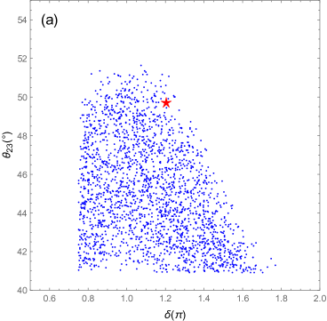
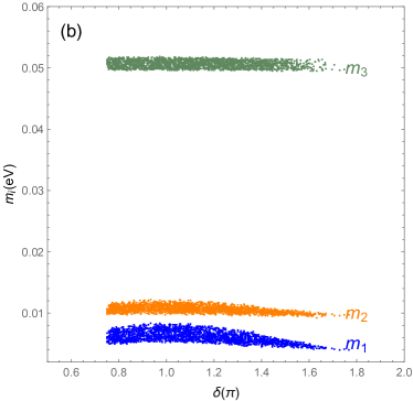
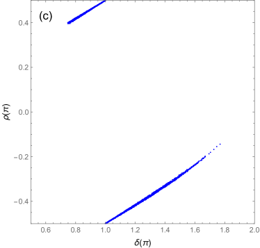
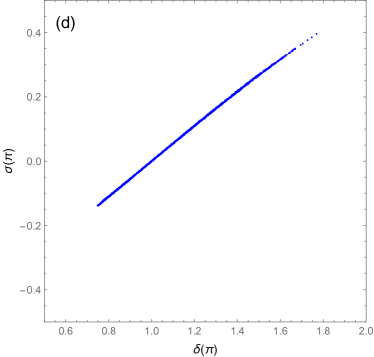
Figure 2: Allowed samples of $A_{1}$ texture with neutrino oscillation data varied in $3\sigma$ range of Ref. Esteban:2018azc . In pattern (a), the red star $\bigstar$ stands for the best fit point from global analysis.

The flavor dependent $U(1)_{B-2L_{e}-L_{\tau}}$ symmetry leads to texture $A_{1}$ Fritzsch:2011qv ; Alcaide:2018vni . Since $(M_{\nu})_{ee}=0$, the predicted effective Majorana neutrino mass $\langle m\rangle_{ee}$ is exactly zero for the neutrinoless double-beta decay. Therefore, only normal hierarchy is allowed Bilenky:1999wz ; Vissani:1999tu . Following the procedure in Ref. Fritzsch:2011qv , we now update the predictions of neutrino oscillation data with latest global analysis results Esteban:2018azc .

In Fig. 2, we show the scanning results of texture $A_{1}$. It is worth to note that the best fit value of neutrino oscillation parameters by global analysis Esteban:2018azc is only marginally consistent with predictions of texture $A_{1}$, which is clearly seen in Fig. 2 (a). From Fig. 2 (b), we obtain that $m_{1}\sim 0.007$ eV, $m_{2}\sim 0.01$ eV, and $m_{3}\approx\sqrt{\Delta m^{2}}\sim 0.05$ eV. The resulting sum of neutrino mass is then $\sum m_{i}\sim 0.07$ eV, thus it satisfies the bound from cosmology, i.e., $\sum m_{i}<0.12$ eV Aghanim:2018eyx . The Dirac phase should fall in the range $\delta\in[0.75\pi,1.77\pi]$, meanwhile Fig. 2 (c) and (d) indicate that $\rho\approx\frac{\delta}{2}$ and $\sigma\approx\frac{\delta}{2}-\frac{\pi}{2}$.

Instead of the marginally best fit value, we take $\delta=\pi$ and $\theta_{23}=46^{\circ}$ with other oscillation parameters being the best fit value in Ref Esteban:2018azc as the benchmark point for illustration, which leads to the following neutrino mass structure

$$M_{\nu}=\left(\begin{array}[]{ccc}0&0&0.0110\\ 0&0.0293&0.0219\\ 0.0110&0.0219&0.0256\end{array}\right)~{}\text{eV}$$ (37)

By comparing the analytic $M_{\nu}$ in Eq. (26) and numerical $M_{\nu}$ in Eq. (37), one can easily reproduce the observed neutrino oscillation data by requiring

$$\frac{h_{\tau 2}}{h_{\mu 1}}:\frac{f_{\tau 1}}{h_{\mu 1}}:\frac{f_{e2}}{h_{\mu 1}} = \frac{(M_{\nu})_{\mu\tau}}{(M_{\nu})_{\mu\mu}}:\sqrt{\frac{(M_{\nu})_{\tau\tau}}{(M_{\nu})_{\mu\mu}}}:\frac{(M_{\nu})_{e\tau}}{\sqrt{(M_{\nu})_{\mu\mu}(M_{\nu})_{\tau\tau}}}$$

$$\simeq 0.745:0.933:0.401.$$

Hence, we can take $h_{\mu 1}$ as free parameters and determine the other three Yukawa coupling by using above ratios. The overall neutrino mass scale is then determined by $\lambda v^{2}M_{N}h_{\mu 1}^{2}/(32\pi^{2}m_{0}^{2})\approx 0.0293$ eV.

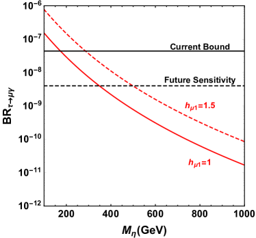
Figure 3: Predictions for $\tau\to\mu\gamma$ (left) and $\tau\to e\gamma$ (right) with corresponding current bound Aubert:2009ag and future sensitivity Hayasaka:2013dsa . In these figures, we have fixed $M_{N_{1}}=200$ GeV.

III.2 Lepton Flavor Violation

The new Yukawa interactions of the form $\bar{L}\tilde{\eta}N_{R}$ will contribute to lepton flavor violation (LFV) processes Toma:2013zsa ; Ding:2014nga . In this work, we take the radiative decay $\ell_{i}\to\ell_{j}\gamma$ for illustration. With flavor dependent $U(1)_{B-2L_{e}-L_{\tau}}$ symmetry, it is clear from Eq. (II.2) that $\eta_{1}^{\pm}(\eta_{2}^{\pm})$ will only induce $\tau\to\mu\gamma(\tau\to e\gamma)$ at one-loop level. It is worth to note that the most stringent $\mu\to e\gamma$ decay is missing at one-loop level. Hence, if the ongoing experiments observe $\tau\to\mu\gamma$ and $\tau\to e\gamma$ but no $\mu\to e\gamma$, this model will be favored. The corresponding branching ratios are calculated as

$$\text{BR}(\tau\to\mu\gamma) = \frac{3\alpha}{64\pi G_{F}^{2}}\left|\sum_{i=1}^{2}\frac{(h_{\mu 1}V_{1i})(h_{\tau 2}V_{2i})^{*}}{M_{\eta_{1}}^{2}}F\left(\frac{M_{Ni}^{2}}{M_{\eta_{1}}^{2}}\right)\right|^{2}\text{BR}(\tau\to\mu\nu_{\tau}\bar{\nu}_{\mu}),$$ (39)

$$\text{BR}(\tau\to e\gamma) = \frac{3\alpha}{64\pi G_{F}^{2}}\left|\sum_{i=1}^{2}\frac{(f_{e2}V_{2i})(f_{\tau 1}V_{1i})^{*}}{M_{\eta_{2}}^{2}}F\left(\frac{M_{Ni}^{2}}{M_{\eta_{2}}^{2}}\right)\right|^{2}\text{BR}(\tau\to e\nu_{\tau}\bar{\nu}_{e}),$$

where the loop function $F(x)$ is

$$F(x)=\frac{1-6x+3x^{2}+2x^{3}-6x^{2}\ln x}{6(1-x)^{4}}.$$ (40)

In the limit for degenerate $M_{N}$, we have

$$\text{BR}(\tau\to\ell\gamma)\propto\left|\sum_{i=1}^{2}V_{1i}V_{2i}^{*}\right|^{2}=|(VV^{\dagger})_{12}|^{2}=0,$$ (41)

where in the last step, we have considered the fact that $V$ is an unitary matrix. Therefore, large cancellations between the contribution of two $N_{i}$ are also possible even in the case of non-degenerate $M_{N}$. In Fig. 3, we show the predictions for $\tau\to\mu\gamma$ and $\tau\to e\gamma$. Although constraint on BR($\tau\to e\gamma$) is slightly more stringent than BR($\tau\to\mu\gamma$), the predicted BR($\tau\to e\gamma$) is much smaller than BR($\tau\to\mu\gamma$). It is clear that the current bound is quite loose, e.g., $M_{\eta}\gtrsim 200$ GeV with $h_{\mu 1}=1$ can be allowed.

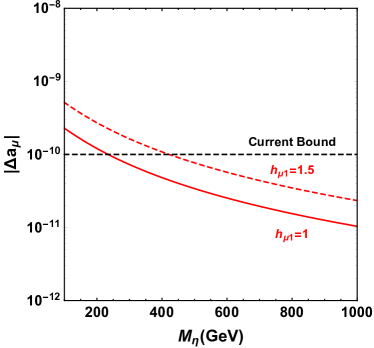
Figure 4: Predictions for $|\Delta a_{\mu}|$. In this figures, we have fix $M_{N_{1}}=200$ GeV.

Although the Yukawa interaction $\bar{L}_{\mu}\tilde{\eta}_{1}N_{i}$ can not induce $\mu\to e\gamma$ at one-loop, it does contribute to muon anomalous magnetic moment Lindner:2016bgg

$$\Delta a_{\mu}=-\sum_{i=1}^{2}\frac{|h_{\mu 1}V_{1i}|^{2}M_{\mu}^{2}}{16\pi^{2}M_{\eta_{1}}^{2}}F\left(\frac{M_{Ni}^{2}}{M_{\eta_{1}}^{2}}\right).$$ (42)

Comparing with BR($\tau\to\ell\gamma$), there is no cancellations between the contribution of two $N_{i}$. However, the total contribution to $\Delta a_{\mu}$ is negative, while the observed discrepancy $\Delta a_{\mu}=a_{\mu}^{\text{EXP}}-a_{\mu}^{\text{SM}}=(261\pm 78)\times 10^{-11}$ is positive Blum:2013xva . Thus, the Yukawa interaction $\bar{L}_{\mu}\tilde{\eta}_{1}N_{R1}$ can not explain the $(g-2)_{\mu}$ anomaly, and some other new physics is required Lindner:2016bgg . On the other hand, since a too large negative contribution to $\Delta a_{\mu}$ is not favored, we consider theoretical $|\Delta a_{\mu}|<10^{-10}$ in the following. The results are shown in Fig. 4. We find that the bound from $|\Delta a_{\mu}|<10^{-10}$ is actually slightly more stringent than BR$(\tau\to\mu\gamma)$.

III.3 Dark Matter

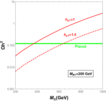
Figure 5: Predicted relic density as a function of $m_{\eta}$, where we have fix $M_{N_{1}}=200$ GeV. The green line corresponds to the observed relic density $\Omega h^{2}=0.120\pm 0.001$ Aghanim:2018eyx .

In this work, we consider $N_{1}$ is the DM candidate. In the original scotogenic model Ma:2006km , the viable annihilation channel is $N_{1}N_{1}\to\ell^{+}\ell^{-},\bar{\nu}\nu$ via the Yukawa interaction $\bar{L}_{\ell}\tilde{\eta}N_{1}$ Kubo:2006yx . However, such annihilation channel is tightly constrained by non-observation of LFV Vicente:2014wga . Thanks to relative loose constraints from $\tau$ decays, the scanning results of Ref. Vicente:2014wga suggested that $N_{1}$ should have a large coupling to $L_{\tau}$. Thus, the dominant annihilation channel is $\tau^{+}\tau^{-}$ and $\bar{\nu}_{\tau}\nu_{\tau}$ with $M_{N_{1}}\lesssim 3$ TeV.

Quite different from the original scotogenic model Ma:2006km , the LFV process is either vanishing or suppressed in this flavor dependent model. Therefore, $\mathcal{O}(1)$ Yukawa coupling can be easily realised without tuning. In the following quantitative investigation, we consider a special scenario, i.e., $M_{\eta_{1}}=M_{\eta_{2}}=M_{\eta}$ for simplicity. For vanishing lepton masses, the Yukawa-portal annihilation cross section is Kubo:2006yx ; Li:2010rb

$$\sigma v_{\text{rel}}=a+bv_{\text{rel}}^{2}=0+\sum_{\alpha,\beta}\left|h^{\prime}_{\alpha 1}h^{\prime*}_{\beta 1}+f^{\prime}_{\alpha 1}f^{\prime*}_{\beta 1}\right|^{2}\frac{r^{2}(1-2r+2r^{2})}{24\pi M_{N_{1}}^{2}}v_{\text{rel}}^{2},$$ (43)

where $v_{\text{rel}}$ is the relative speed, $h^{\prime}$ and $f^{\prime}$ are defined in Eq. (33), $r=M_{N_{1}}^{2}/(M_{\eta}^{2}+M_{N_{1}}^{2})$. The thermally averaged cross section is calculated as $\langle\sigma v_{\text{rel}}\rangle=a+6b/x_{f}$, where the freeze-out parameter $x_{f}=M_{N_{1}}/T_{f}$ is obtained by numerically solving

$$x_{f}=\ln\left(\frac{0.038M_{\text{Pl}}M_{N_{1}}\langle\sigma v_{\text{rel}}\rangle}{\sqrt{g_{*}x_{f}}}\right).$$ (44)

The relic density is then calculated as Bertone:2004pz

$$\Omega h^{2}=\frac{1.07\times 10^{9}{\rm GeV}^{-1}}{M_{\text{Pl}}}\frac{x_{f}}{\sqrt{g_{*}}}\frac{1}{a+3b/x_{f}},$$ (45)

where $M_{\text{Pl}}=1.22\times 10^{19}$ GeV is the Planck mass, $g_{*}$ is the number of relativistic degrees of freedom. The numerical results are depicted in Fig 5. Provided the mass of the DM candidate is $M_{N_{1}}=200$ GeV, then the observed relic density is interpreted by $h_{\mu 1}=1,M_{\eta}=366$ GeV or $h_{\mu 1}=1.5,M_{\eta}=640$ GeV. That is to say, $h_{\mu 1}\sim\mathcal{O}(1)$ is required to obtain correct relic density, and the larger $h_{\mu 1}$ is, the larger the mass splitting $M_{\eta}-M_{N_{1}}$ is.

In addition to the Yukawa-portal interaction, $N_{1}$ can also annihilate via the Higgs-portal and $Z^{\prime}$-portal interactions Okada:2010wd ; Kanemura:2011vm ; Okada:2012sg ; Wang:2015saa ; Okada:2016gsh ; Okada:2018ktp ; Han:2018zcn . In these two scenarios, $M_{N_{1}}\simeq M_{h,H}/2$ or $\simeq M_{Z^{\prime}}/2$ are usually required to realize correct relic density Borah:2018smz . If the additional scalar singlet scalar $H$ is lighter than $N_{1}$, then the annihilation channel $N_{1}N_{1}\to HH$ with $H\to b\bar{b}$ is able to explain the Fermi-LAT gamma-ray excess at the Galactic center Kim:2016csm ; Ding:2018jdk .

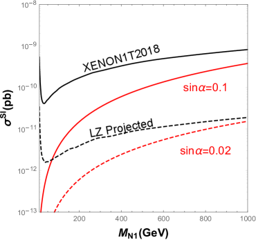
Figure 6: Spin-independent cross section as a function of $M_{N_{1}}$. The black solid and dashed line correspond to current XENON1T Aprile:2018dbl and future LZ Akerib:2018lyp limits, respectively. In this figure, we have set $M_{H_{1}}=500$ GeV and $v_{S}=10$ TeV.

The spin-independent DM-nucleon scattering cross section is dominantly mediated by scalar interactions, which is given by

$$\sigma^{\text{SI}}=\frac{4}{\pi}\left(\frac{M_{p}M_{N_{1}}}{M_{p}+M_{N_{1}}}\right)^{2}f_{p}^{2},$$ (46)

where $M_{p}$ is the proton mass and the hadronic matrix element $f_{p}$ reads

$$\frac{f_{p}}{M_{p}}=\sum_{q=u,d,s}f^{p}_{Tq}\frac{\alpha_{q}}{M_{q}}+\frac{2}{27}\left(1-\sum_{q=u,d,s}f^{p}_{Tq}\right)\sum_{q=c,b,t}\frac{\alpha_{q}}{M_{q}}.$$ (47)

and the effective vertex

$$\frac{\alpha_{q}}{M_{q}}=-\frac{y_{N_{1}}}{\sqrt{2}v}\sin 2\alpha\left(\frac{1}{M_{h}^{2}}-\frac{1}{M_{H_{1}}^{2}}\right),$$ (48)

Here, $y_{N_{1}}=y_{11}V_{11}^{2}$ is the effective Yukawa coupling of $N_{1}$ with $S_{1}$. For proton, the parameters $f^{p}_{Tq}$ are evaluated as $f^{p}_{Tu}=0.020\pm 0.004$, $f^{p}_{Td}=0.026\pm 0.005$ and $f^{p}_{Ts}=0.118\pm 0.062$ Ellis:2000ds . Fig. 6 shows the numerical results for direct detection. It is obvious that the predicted $\sigma^{\text{SI}}$ with $\sin\alpha=0.1$ lies below current XENON1T limit, but the range of $M_{N_{1}}\gtrsim 70$ GeV is within future LZ’s reach. However, if no direct detection signal is observed by LZ, then $\sin\alpha\lesssim 0.02$ should be satisfied.

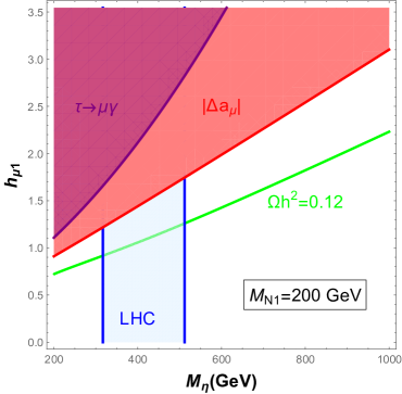
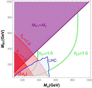
Figure 7: Combined results for the Yukawa-portal DM. Left pattern: in the $h_{\mu 1}$-$M_{\eta}$ plane; right pattern: in the $M_{N_{1}}$-$M_{\eta}$ plane. The green lines satisfy the condition for correct relic density. And the blue regions are excluded by LHC direct search, which will be discussed in Sec. III.4.

In Fig. 7, we show the combined results from LFV, $|\Delta a_{\mu}|$, relic density and LHC search. In left pattern of Fig. 7, it indicates that for $M_{N_{1}}=200$ GeV, the only exclusion region is from LHC search. Hence, either $M_{\eta}\lesssim 300$ GeV with $h_{\mu 1}\lesssim 0.9$ or $M_{\eta}\gtrsim 500$ GeV with $h_{\mu 1}\gtrsim 1.3$ is required. In right pattern of Fig. 7, two benchmark value $h_{\mu 1}=1.0,1.5$ are chosen to illustrate. For $h_{\mu 1}=1.0$, we have $250~{}\text{GeV}\lesssim M_{N_{1}}\lesssim M_{\eta}\sim 400$ GeV. Therefore, the only viable region is $M_{N_{1}}\sim M_{\eta}\lesssim 400$ GeV for $h_{\mu 1}\lesssim 1$. Meanwhile for $h_{\mu 1}=1.5$, $M_{N_{1}}\gtrsim 120$ GeV with $M_{\eta}\gtrsim 520$ GeV is able to escape LHC limit.

III.4 Collider Signature

In this part, we highlight some interesting collider signatures. Begin with the newly discovered 125 GeV Higgs boson $h$ Aad:2012tfa ; Chatrchyan:2012xdj . The existence of massless Mojoron $J$ will induce the invisible decay of SM Higgs via $h\to JJ$ Wang:2016vfj . The corresponding decay width is evaluated as

$$\Gamma(h\to JJ)\simeq\frac{M_{h}^{3}\sin^{2}\alpha}{32\pi v_{S}^{2}}.$$ (49)

Then, the branching ratio of invisible decay is BR($h\to JJ)=\Gamma(h\to JJ)/(\Gamma(h\to JJ)+\Gamma_{\text{SM}}\cos^{2}\alpha)$, where $\Gamma_{\text{SM}}=4.09$ MeV deFlorian:2016spz . Currently, the combined direct and indirect observational limit on invisible Higgs decay is BR($h\to JJ)<0.24$ Khachatryan:2016whc . Typically for $\sin\alpha=0.1,v_{S}=10$ TeV, we have BR($h\to JJ)=4.8\times 10^{-4}$, which is far below current limit. Meanwhile, if $M_{H_{1}}<2M_{h}$, then $h\to H_{1}H_{1}$ with $H_{1}\to JJ$ will also contribute to invisible Higgs decay  Bonilla:2015uwa .

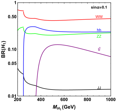
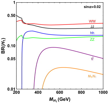
Figure 8: Branching ratios of scalar singlet $H_{1}$ for $\sin\alpha=0.1$(left) and $\sin\alpha=0.02$(right). In this figures, we have also fix $M_{N_{1}}=200$ GeV and $v_{S}=10$ TeV. Note in left pattern, BR$(H_{1}\to N_{1}N_{1})$ is less than 0.01, thus is not shown in the plot.

In this paper, we consider the high mass scenario $M_{H_{1}}>M_{h}$. In addition to the usual $H_{1}\to$ SM final states as real singlet model Robens:2016xkb , the heavy scalar singlet can also decay into Majoron pair $H_{1}\to JJ$ and DM pair $H_{1}\to N_{1}N_{1}$. Fig. 8 shows the dominant decay branching ratios of $H_{1}$. The invisible BR$(H_{1}\to JJ)$ is less than 0.02 when $\sin\alpha=0.1$, therefore $H_{1}$ appears as a SM heavy Higgs with BR$(H_{1}\to hh)\approx\text{BR}(h\to ZZ)\approx\frac{1}{2}\text{BR}(H_{1}\to WW)\approx\frac{1}{4}$. While for $\sin\alpha=0.02$, the invisible BR$(H_{1}\to JJ)$ increases to about $0.25$, reaching the same order of visible $VV,hh$ decay. And the other invisible decay $H_{1}\to N_{1}N_{1}$ maximally reaches about $0.03$ at $M_{H_{1}}\sim 600$ GeV. The dominant production channel of $H_{1}$ is via gluon fusion at LHC, which can be estimated as

$$\sigma(gg\to H_{1})\approx\sin^{2}\alpha\times\sigma(gg\to h),$$ (50)

where $\sigma(gg\to h)$ is the SM Higgs production cross section but calculated with $M_{h}=M_{H_{1}}$. At present, $\sin\alpha\sim 0.1$ Ilnicka:2018def leads to the promising signatures as $H_{1}\to WW\to e\nu\mu\nu$ Aaboud:2017gsl , $ZZ\to 4\ell$ Aaboud:2018bun and $hh\to 2b2\gamma$ Sirunyan:2018iwt ; Aaboud:2018ftw , etc. In the future, if no DM direct detection signal is observed, then the signature of heavy scalar $H_{1}$ will be much suppressed by tiny value of $\sin\alpha$.

$q\bar{q}$	$e^{+}e^{-}$	$\mu^{+}\mu^{-}$	$\tau^{+}\tau^{-}$	$\nu\nu$	$NN$	$H_{1}H_{1}$
0.154	0.308	0	0.077	0.192	0.192	0.077

Table 3: Decay branching ratio of $U(1)_{B-2L_{e}-L_{\tau}}$ gauge boson $Z^{\prime}$, where we have show the lepton flavor individually.

Next, we discuss the gauge boson $Z^{\prime}$ associated with $U(1)_{B-2L_{e}-L_{\tau}}$. Its decay branching ratios are flavor-dependent, which makes it quite easy to distinguish from the flavor-universal ones, such as $Z^{\prime}$ from $U(1)_{B-L}$ Basso:2008iv . Considering the heavy $Z^{\prime}$ limit, its partial decay width into fermion and scalar pairs are given by

$$\Gamma(Z^{\prime}\to f\bar{f}) = \frac{M_{Z^{\prime}}}{24\pi}g^{\prime 2}N_{C}^{f}(Q_{fL}^{2}+Q_{fR}^{2}),$$ (51)

$$\Gamma(Z^{\prime}\to SS^{*}) = \frac{M_{Z^{\prime}}}{48\pi}g^{\prime 2}Q_{S}^{2},$$ (52)

where $N_{C}^{f}$ is the number of colours of the fermion $f$, i.e., $N_{C}^{l,\nu}=1$, $N_{C}^{q}=3$, and $Q_{X}$ is the $U(1)_{B-2L_{e}-L_{\tau}}$ charge of particle $X$. In Tab. 3, we present the branching ratio of $Z^{\prime}$. The dominant channel is $Z^{\prime}\to e^{+}e^{-}$ with branching ratio of $0.308$, and no $Z^{\prime}\to\mu^{+}\mu^{-}$. The $B-2L_{e}-L_{\tau}$ nature of $Z^{\prime}$ predicts definite relation between quark and lepton final states, e.g.,

$$\text{BR}(Z^{\prime}\to b\bar{b}):\text{BR}(Z^{\prime}\to e^{+}e^{-}):\text{BR}(Z^{\prime}\to\mu^{+}\mu^{-}):\text{BR}(Z^{\prime}\to\tau^{+}\tau^{-})=\frac{1}{3}:4:0:1,$$ (53)

which is also an intrinsic property to distinguish $Z^{\prime}$ of $U(1)_{B-2L_{e}-L_{\tau}}$ from other flavored gauge bosons Chun:2018ibr .

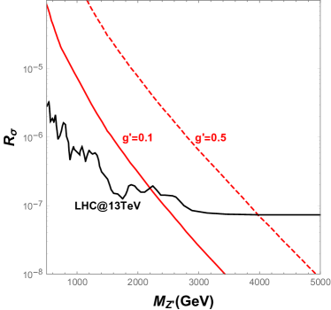
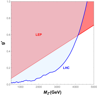
Figure 9: Left pattern: predicted cross section ratios in $U(1)_{B-2L_{e}-L_{\tau}}$ and corresponding limit from LHC. Right pattern: allowed parameter space in the $g^{\prime}$-$M_{Z^{\prime}}$ plane.

In the framework of $U(1)_{B-2L_{e}-L_{\tau}}$, one important constraint on $Z^{\prime}$ comes from the precise measurement of four-fermion interactions at LEP Cacciapaglia:2006pk , which requires

$$\frac{M_{Z^{\prime}}}{g^{\prime}}\gtrsim 7~{}{\rm TeV}.$$ (54)

Since $Z^{\prime}$ couples to both quarks and leptons, the most promising signature at LHC is the dilepton signature $pp\to Z^{\prime}\to e^{+}e^{-}$. Searches for such dilepton signature have been performed by ATLAS Aaboud:2017buh and CMS collaboration Sirunyan:2018exx . Because of no $Z^{\prime}\to\mu^{+}\mu^{-}$ channel, we can only take the results from CMS, which provides a limit on the ratio

$$R_{\sigma}=\frac{\sigma(pp\to Z^{\prime}+X\to e^{+}e^{-}+X)}{\sigma(pp\to Z+X\to e^{+}e^{-}+X)}.$$ (55)

The theoretical cross section of the dilepton signature are calculated by using MadGraph5_aMC@NLO Alwall:2014hca . Left pattern of Fig. 9 shows that the dilepton signature has excluded $M_{Z^{\prime}}\lesssim 2.2(4.0)$ TeV for $g^{\prime}=0.1(0.5)$. Then comparing the theoretical ratio with experimental limit, one can acquire the exclusion limit in the $g^{\prime}-M_{Z^{\prime}}$ plane as shown in right pattern of Fig. 9. Obviously, LHC limit is more stringent than LEP when $M_{Z^{\prime}}\lesssim 4$ TeV.

The inert charge scalars $\eta_{1,2}^{\pm}$ are also observable at LHC. They can decay into charged leptons and right-hand singlets via the Yukawa interactions as

$$\Gamma(\eta^{\pm}_{1}\to\ell^{\pm}N_{i}) = \frac{M_{\eta_{1}^{\pm}}}{16\pi}\left|h^{\prime}_{\ell i}\right|^{2}\left(1-\frac{M_{N_{i}}^{2}}{M_{\eta^{\pm}_{1}}^{2}}\right)^{2},$$ (56)

$$\Gamma(\eta^{\pm}_{2}\to\ell^{\pm}N_{i}) = \frac{M_{\eta_{1}^{\pm}}}{16\pi}\left|f^{\prime}_{\ell i}\right|^{2}\left(1-\frac{M_{N_{i}}^{2}}{M_{\eta^{\pm}_{2}}^{2}}\right)^{2}.$$ (57)

From Eq. (II.2), we aware that $\eta_{1}^{\pm}$ decays into $\mu,\tau$ final states, while $\eta_{2}^{\pm}$ decays into $e,\tau$ final states. The electron-phobic nature of $\eta_{1}^{\pm}$ and muon-phobic nature of $\eta_{2}^{\pm}$ make them quite easy to distinguish. Meanwhile, their decay branching ratios are related by neutrino oscillation data through the Yukawa coupling $h^{\prime},f^{\prime}$. Considering the benchmark point in Eq. (III.1), the predicted branching ratios are shown in Tab.  4 in the heavy scalar limit. The dominant decay channel of $\eta^{\pm}_{1}$ is $\mu^{\pm}N_{1}$, and $\tau^{\pm}N_{1}$ for $\eta^{\pm}_{2}$. So $\eta^{\pm}_{1}$ is expected easier to be discovered. Produced via the Drell-Yan process $pp\to\eta^{+}_{1}\eta^{-}_{1},\eta^{+}_{2}\eta^{-}_{2}$, the decay channel $\eta^{\pm}_{1,2}\to\ell^{\pm}N_{1}$ then leads to signature $\ell^{+}\ell^{-}+\cancel{E}_{T}$. Exclusion region by direct LHC search for such signature Aaboud:2018jiw has been shown in right pattern of Fig. 7. To satisfy the direct LHC search bounds, one needs either $M_{N_{1}}\lesssim M_{\eta}<500$ GeV or $M_{\eta}>500$ GeV.

Final state	$e^{\pm}N_{1}$	$\mu^{\pm}N_{1}$	$\tau^{\pm}N_{1}$	$e^{\pm}N_{2}$	$\mu^{\pm}N_{2}$	$\tau^{\pm}N_{2}$
$\eta^{\pm}_{1}$	0.000	0.465	0.099	0.000	0.178	0.258
$\eta^{\pm}_{2}$	0.043	0.000	0.611	0.113	0.000	0.233

Table 4: Branching ratios of charge scalar $\eta_{1,2}^{\pm}$.

IV Conclusion

The scotogenic model is an elegant pathway to explain the origin of neutrino mass and dark matter. Meanwhile, texture-zeros in neutrino mass matrix provide a promising way to under stand the leptonic flavor structure. Therefore, it is appealing to connect the scotogenic model with texture-zeros. In this paper, we propose a viable approach to realise two texture-zeros in the scotogenic model with flavor dependent $U(1)_{B-2L_{\alpha}-L_{\beta}}$ gauge symmetry. These models are extended by two right-handed singlets $N_{Ri}$ and two inert scalar doublets $\eta_{i}$, which are odd under the dark $Z_{2}$ symmetry. Six kinds of texture-zeros are realised in our approach, i.e., texture $A_{1}$, $A_{2}$, $B_{3}$, $B_{4}$, $D_{1}$ and $D_{2}$. Among all the six texture-zeros, we find that texture $A_{1}$ and $A_{2}$ are allowed by current experimental limits, while texture $B_{3}$ and $B_{4}$ are marginally allowed. Besides, texture $D_{1}$ and $D_{2}$ are already excluded by neutrino oscillation data.

Realization of texture-zeros in the scotogenic model makes the model quite predictive. And we have taken texture $A_{1}$ derived from $U(1)_{B-2L_{e}-L_{\tau}}$ for illustration. Some distinct features are summarized in the following:

• The texture $A_{1}$ predicts vanishing neutrinoless double beta decay rate. And only normal neutrino mass hierarchy is allowed. It predicts $m_{1}\sim 0.007$ eV, $m_{2}\sim 0.01$ eV, and $m_{3}\approx\sqrt{\Delta m^{2}}\sim 0.05$ eV, then $\sum m_{i}\sim 0.07$ eV. There are also strong correlation between the Dirac and Majorana phases, i.e., $\rho\approx\frac{\delta}{2}$ and $\sigma\approx\frac{\delta}{2}-\frac{\pi}{2}$.

• The ratios of corresponding Yukawa couplings are also predicted by neutrino oscillation data, e.g.,

  $$\frac{h_{\tau 2}}{h_{\mu 1}}:\frac{f_{\tau 1}}{h_{\mu 1}}:\frac{f_{e2}}{h_{\mu 1}}\simeq 0.745:0.933:0.401.$$

• Due to specific Yukawa structure, the LFV process $\mu\to e\gamma$ is missing at one-loop level. Meanwhile, large cancellations are possible for $\tau\to\mu\gamma$ and $\tau\to e\gamma$ with degenerate right-handed singlets. More stringent constraint comes from muon anomalous magnetic moment $\Delta a_{\mu}$. Although $\mathcal{O}(1)$ Yukawa couplings are easily to avoid such limit.

• Satisfying all constraints, correct relic density of dark matter $N_{1}$ is achieved for $M_{N_{1}}\lesssim M_{\eta}<500$ GeV with $h_{\mu 1}\lesssim 1$ or $M_{\eta}>500$ GeV with $h_{\mu 1}>1$.As for direct detection, we have shown that the predicted spin-independent DM-nucleon cross section $\sigma^{\text{SI}}$ with $\sin\alpha=0.1$ satisfies the current XENON1T limit, but is within future reach of LZ.

• The massless Mojoron $J$ contributes to invisible decay of SM Higgs. The additional scalr singlet $H_{1}$ can be probe in the channel $gg\to H_{1}\to W^{+}W^{-},ZZ$ at LHC. Decays of charged scalars $\eta_{1,2}^{\pm}$ lead to $pp\to\eta^{+}_{1,2}\eta^{-}_{1,2}\to\ell^{+}\ell^{-}+\cancel{E}_{T}$ signature. Note that the corresponding branching ratios are also correlated with neutrino oscillation parameters.

• The neutral gauge boson $Z^{\prime}$ is promising via the di-electron signature $pp\to Z^{\prime}\to e^{+}e^{-}$. Its $B-2L_{e}-L_{\tau}$ nature can be confirmed by

  $$\text{BR}(Z^{\prime}\to b\bar{b}):\text{BR}(Z^{\prime}\to e^{+}e^{-}):\text{BR}(Z^{\prime}\to\mu^{+}\mu^{-}):\text{BR}(Z^{\prime}\to\tau^{+}\tau^{-})=\frac{1}{3}:4:0:1,$$

In a nutshell, the scotogenic model with flavor dependent $U(1)_{B-2L_{\alpha}-L_{\beta}}$ symmetry predicts distinct and observable phenomenology, which is useful to distinguish from other models.

V Acknowledgements

The work of Weijian Wang is supported by National Natural Science Foundation of China under Grant Numbers 11505062, Special Fund of Theoretical Physics under Grant Numbers 11447117 and Fundamental Research Funds for the Central Universities under Grant Numbers 2014ZD42. The work of Zhi-Long Han is supported by National Natural Science Foundation of China under Grant No. 11805081 and No. 11605075, Natural Science Foundation of Shandong Province under Grant No. ZR2018MA047, No. ZR2017JL006 and No. ZR2014AM016.

References

- (1) E. Ma, Phys. Rev. D 73, 077301 (2006) [hep-ph/0601225].
- (2) L. M. Krauss, S. Nasri and M. Trodden, Phys. Rev. D 67, 085002 (2003) [hep-ph/0210389].
- (3) M. Aoki, S. Kanemura and O. Seto, Phys. Rev. Lett. 102, 051805 (2009) [arXiv:0807.0361 [hep-ph]].
- (4) E. Ma, Mod. Phys. Lett. A 21, 1777 (2006) [hep-ph/0605180].
- (5) T. Hambye, K. Kannike, E. Ma and M. Raidal, Phys. Rev. D 75, 095003 (2007) [hep-ph/0609228].
- (6) D. Aristizabal Sierra, J. Kubo, D. Restrepo, D. Suematsu and O. Zapata, Phys. Rev. D 79, 013011 (2009) [arXiv:0808.3340 [hep-ph]].
- (7) D. Suematsu, T. Toma and T. Yoshida, Phys. Rev. D 79, 093004 (2009) [arXiv:0903.0287 [hep-ph]].
- (8) D. Schmidt, T. Schwetz and T. Toma, Phys. Rev. D 85, 073009 (2012) [arXiv:1201.0906 [hep-ph]].
- (9) R. Bouchand and A. Merle, JHEP 1207, 084 (2012) [arXiv:1205.0008 [hep-ph]]. A. Merle and M. Platscher, JHEP 1511, 148 (2015) [arXiv:1507.06314 [hep-ph]].
- (10) E. Ma, A. Natale and A. Rashed, Int. J. Mod. Phys. A 27, 1250134 (2012) [arXiv:1206.1570 [hep-ph]].
- (11) M. Klasen, C. E. Yaguna, J. D. Ruiz-Alvarez, D. Restrepo and O. Zapata, JCAP 1304, 044 (2013) [arXiv:1302.5298 [hep-ph]].
- (12) S. Y. Ho and J. Tandean, Phys. Rev. D 87, 095015 (2013) [arXiv:1303.5700 [hep-ph]].
- (13) K. P. Modak, JHEP 1503, 064 (2015) [arXiv:1404.3676 [hep-ph]].
- (14) E. Molinaro, C. E. Yaguna and O. Zapata, JCAP 1407, 015 (2014) [arXiv:1405.1259 [hep-ph]].
- (15) G. Faisel, S. Y. Ho and J. Tandean, Phys. Lett. B 738, 380 (2014) [arXiv:1408.5887 [hep-ph]].
- (16) A. Merle and M. Platscher, Phys. Rev. D 92, no. 9, 095002 (2015) [arXiv:1502.03098 [hep-ph]].
- (17) A. Ahriche, K. L. McDonald and S. Nasri, JHEP 1606, 182 (2016) [arXiv:1604.05569 [hep-ph]].
- (18) M. Lindner, M. Platscher, C. E. Yaguna and A. Merle, Phys. Rev. D 94, no. 11, 115027 (2016) [arXiv:1608.00577 [hep-ph]].
- (19) A. G. Hessler, A. Ibarra, E. Molinaro and S. Vogl, JHEP 1701, 100 (2017) [arXiv:1611.09540 [hep-ph]].
- (20) D. Borah and A. Gupta, Phys. Rev. D 96, no. 11, 115012 (2017) [arXiv:1706.05034 [hep-ph]].
- (21) A. Abada and T. Toma, JHEP 1804, 030 (2018) [arXiv:1802.00007 [hep-ph]].
- (22) T. Hugle, M. Platscher and K. Schmitz, Phys. Rev. D 98, no. 2, 023020 (2018) [arXiv:1804.09660 [hep-ph]].
- (23) S. Baumholzer, V. Brdar and P. Schwaller, JHEP 1808, 067 (2018) [arXiv:1806.06864 [hep-ph]].
- (24) D. Borah, P. S. B. Dev and A. Kumar, arXiv:1810.03645 [hep-ph].
- (25) L. Bian and X. Liu, arXiv:1811.03279 [hep-ph].
- (26) Y. Cai, J. Herrero-García, M. A. Schmidt, A. Vicente and R. R. Volkas, Front. in Phys. 5, 63 (2017) [arXiv:1706.08524 [hep-ph]].
- (27) P. H. Frampton, S. L. Glashow and D. Marfatia, Phys. Lett. B 536, 79 (2002) [hep-ph/0201008].
- (28) H. Fritzsch, Z. z. Xing and S. Zhou, JHEP 1109, 083 (2011) [arXiv:1108.4534 [hep-ph]].
- (29) J. Alcaide, J. Salvado and A. Santamaria, JHEP 1807, 164 (2018) [arXiv:1806.06785 [hep-ph]].
- (30) W. Grimus, A. S. Joshipura, L. Lavoura and M. Tanimoto, Eur. Phys. J. C 36, 227 (2004) [hep-ph/0405016].
- (31) T. Araki, J. Heeck and J. Kubo, JHEP 1207, 083 (2012) [arXiv:1203.4951 [hep-ph]].
- (32) L. M. Cebola, D. Emmanuel-Costa and R. Gonzalez Felipe, Phys. Rev. D 88, no. 11, 116008 (2013) [arXiv:1309.1709 [hep-ph]].
- (33) T. Kitabayashi, Phys. Rev. D 98, no. 8, 083011 (2018) [arXiv:1808.01060 [hep-ph]].
- (34) T. Kitabayashi, S. Ohkawa and M. Yasuè, Int. J. Mod. Phys. A 32, no. 32, 1750186 (2017) [arXiv:1703.09417 [hep-ph]].
- (35) S. Baek, H. Okada and K. Yagyu, JHEP 1504, 049 (2015) [arXiv:1501.01530 [hep-ph]].
- (36) S. Baek, Phys. Lett. B 756, 1 (2016) [arXiv:1510.02168 [hep-ph]].
- (37) S. Lee, T. Nomura and H. Okada, Nucl. Phys. B 931, 179 (2018) [arXiv:1702.03733 [hep-ph]].
- (38) K. Asai, K. Hamaguchi, N. Nagata, S. Y. Tseng and K. Tsumura, arXiv:1811.07571 [hep-ph].
- (39) T. Nomura and H. Okada, Phys. Dark Univ. 21, 90 (2018) [arXiv:1712.00941 [hep-ph]].
- (40) P. Ko, T. Nomura and H. Okada, Phys. Lett. B 772, 547 (2017) [arXiv:1701.05788 [hep-ph]].
- (41) T. Nomura and H. Okada, arXiv:1806.09957 [hep-ph].
- (42) N. Aghanim et al. [Planck Collaboration], arXiv:1807.06209 [astro-ph.CO].
- (43) I. Esteban, M. C. Gonzalez-Garcia, A. Hernandez-Cabezudo, M. Maltoni and T. Schwetz, arXiv:1811.05487 [hep-ph].
- (44) E. Ma, I. Picek and B. Radovčić, Phys. Lett. B 726, 744 (2013) [arXiv:1308.5313 [hep-ph]].
- (45) S. M. Bilenky, C. Giunti, W. Grimus, B. Kayser and S. T. Petcov, Phys. Lett. B 465, 193 (1999) [hep-ph/9907234].
- (46) F. Vissani, JHEP 9906, 022 (1999) [hep-ph/9906525].
- (47) T. Toma and A. Vicente, JHEP 1401, 160 (2014) [arXiv:1312.2840 [hep-ph]].
- (48) R. Ding, Z. L. Han, Y. Liao, H. J. Liu and J. Y. Liu, Phys. Rev. D 89, no. 11, 115024 (2014) [arXiv:1403.2040 [hep-ph]].
- (49) B. Aubert et al. [BaBar Collaboration], Phys. Rev. Lett. 104, 021802 (2010) [arXiv:0908.2381 [hep-ex]].
- (50) K. Hayasaka [Belle and Belle-II Collaborations], J. Phys. Conf. Ser. 408, 012069 (2013).
- (51) M. Lindner, M. Platscher and F. S. Queiroz, Phys. Rept. 731, 1 (2018) [arXiv:1610.06587 [hep-ph]].
- (52) T. Blum, A. Denig, I. Logashenko, E. de Rafael, B. L. Roberts, T. Teubner and G. Venanzoni, arXiv:1311.2198 [hep-ph].
- (53) J. Kubo, E. Ma and D. Suematsu, Phys. Lett. B 642, 18 (2006) [hep-ph/0604114].
- (54) A. Vicente and C. E. Yaguna, JHEP 1502, 144 (2015) [arXiv:1412.2545 [hep-ph]].
- (55) T. Li and W. Chao, Nucl. Phys. B 843, 396 (2011) [arXiv:1004.0296 [hep-ph]].
- (56) G. Bertone, D. Hooper and J. Silk, Phys. Rept. 405, 279 (2005) [hep-ph/0404175].
- (57) N. Okada and O. Seto, Phys. Rev. D 82, 023507 (2010) [arXiv:1002.2525 [hep-ph]].
- (58) S. Kanemura, O. Seto and T. Shimomura, Phys. Rev. D 84, 016004 (2011) [arXiv:1101.5713 [hep-ph]].
- (59) N. Okada and Y. Orikasa, Phys. Rev. D 85, 115006 (2012) [arXiv:1202.1405 [hep-ph]].
- (60) W. Wang and Z. L. Han, Phys. Rev. D 92, 095001 (2015) [arXiv:1508.00706 [hep-ph]].
- (61) N. Okada and S. Okada, Phys. Rev. D 93, no. 7, 075003 (2016) [arXiv:1601.07526 [hep-ph]].
- (62) S. Okada, Adv. High Energy Phys. 2018, 5340935 (2018) [arXiv:1803.06793 [hep-ph]].
- (63) Z. L. Han and W. Wang, Eur. Phys. J. C 78, no. 10, 839 (2018) [arXiv:1805.02025 [hep-ph]].
- (64) D. Borah, D. Nanda, N. Narendra and N. Sahu, arXiv:1810.12920 [hep-ph].
- (65) Y. G. Kim, K. Y. Lee, C. B. Park and S. Shin, Phys. Rev. D 93, no. 7, 075023 (2016) [arXiv:1601.05089 [hep-ph]].
- (66) R. Ding, Z. L. Han, L. Huang and Y. Liao, Chin. Phys. C 42, no. 10, 103101 (2018) [arXiv:1802.05248 [hep-ph]].
- (67) J. R. Ellis, A. Ferstl and K. A. Olive, Phys. Lett. B 481, 304 (2000) [hep-ph/0001005].
- (68) E. Aprile et al. [XENON Collaboration], Phys. Rev. Lett. 121, no. 11, 111302 (2018) [arXiv:1805.12562 [astro-ph.CO]].
- (69) D. S. Akerib et al. [LUX-ZEPLIN Collaboration], arXiv:1802.06039 [astro-ph.IM].
- (70) M. Aaboud et al. [ATLAS Collaboration], JHEP 1710, 182 (2017) [arXiv:1707.02424 [hep-ex]].
- (71) M. Aaboud et al. [ATLAS Collaboration], Eur. Phys. J. C 78, no. 12, 995 (2018) [arXiv:1803.02762 [hep-ex]].
- (72) G. Aad et al. [ATLAS Collaboration], Phys. Lett. B 716, 1 (2012) [arXiv:1207.7214 [hep-ex]].
- (73) S. Chatrchyan et al. [CMS Collaboration], Phys. Lett. B 716, 30 (2012) [arXiv:1207.7235 [hep-ex]].
- (74) W. Wang and Z. L. Han, Phys. Rev. D 94, no. 5, 053015 (2016) [arXiv:1605.00239 [hep-ph]].
- (75) D. de Florian et al. [LHC Higgs Cross Section Working Group], arXiv:1610.07922 [hep-ph].
- (76) V. Khachatryan et al. [CMS Collaboration], JHEP 1702, 135 (2017) [arXiv:1610.09218 [hep-ex]].
- (77) C. Bonilla, J. W. F. Valle and J. C. Romão, Phys. Rev. D 91, no. 11, 113015 (2015) [arXiv:1502.01649 [hep-ph]].
- (78) T. Robens and T. Stefaniak, Eur. Phys. J. C 76, no. 5, 268 (2016) [arXiv:1601.07880 [hep-ph]].
- (79) A. Ilnicka, T. Robens and T. Stefaniak, Mod. Phys. Lett. A 33, no. 10n11, 1830007 (2018) [arXiv:1803.03594 [hep-ph]].
- (80) M. Aaboud et al. [ATLAS Collaboration], Eur. Phys. J. C 78, no. 1, 24 (2018) [arXiv:1710.01123 [hep-ex]].
- (81) M. Aaboud et al. [ATLAS Collaboration], Phys. Rev. D 98, no. 5, 052008 (2018) [arXiv:1808.02380 [hep-ex]].
- (82) A. M. Sirunyan et al. [CMS Collaboration], Phys. Lett. B 788, 7 (2019) [arXiv:1806.00408 [hep-ex]].
- (83) M. Aaboud et al. [ATLAS Collaboration], JHEP 1811, 040 (2018) [arXiv:1807.04873 [hep-ex]].
- (84) L. Basso, A. Belyaev, S. Moretti and C. H. Shepherd-Themistocleous, Phys. Rev. D 80, 055030 (2009) [arXiv:0812.4313 [hep-ph]].
- (85) E. J. Chun, A. Das, J. Kim and J. Kim, arXiv:1811.04320 [hep-ph].
- (86) G. Cacciapaglia, C. Csaki, G. Marandella and A. Strumia, Phys. Rev. D 74, 033011 (2006) [hep-ph/0604111].
- (87) A. M. Sirunyan et al. [CMS Collaboration], JHEP 1806, 120 (2018) [arXiv:1803.06292 [hep-ex]].
- (88) J. Alwall et al., JHEP 1407, 079 (2014) [arXiv:1405.0301 [hep-ph]].