Extracting the pomeron-pomeron-$f_{2}(1270)$ coupling in the $pp\to pp\pi^{+}\pi^{-}$ reaction through angular distributions of the pions

Abstract

We discuss how to extract the pomeron-pomeron-$f_{2}(1270)$ ($\mathbb{P}\mathbb{P}f_{2}(1270)$) coupling within the tensor-pomeron model. The general $\mathbb{P}\mathbb{P}f_{2}(1270)$ coupling is a combination of seven basic couplings (tensorial structures). To study these tensorial structures we propose to measure the central-exclusive production of a $\pi^{+}\pi^{-}$ pair in the invariant mass region of the $f_{2}(1270)$ meson. An analysis of angular distributions in the $\pi^{+}\pi^{-}$ rest system, using the Collins-Soper (CS) and the Gottfried-Jackson (GJ) frames, turns out to be particularly relevant for our purpose. For both frames the $\cos\theta_{\pi^{+}}$ and $\phi_{\pi^{+}}$ distributions are discussed. We find that the azimuthal angle distributions in these frames are fairly sensitive to the choice of the $\mathbb{P}\mathbb{P}f_{2}$ coupling. We show results for the resonance case alone as well as when the dipion continuum is included. We show the influence of the experimental cuts on the angular distributions in the context of dedicated experimental studies at RHIC and LHC energies. Absorption corrections are included for our final distributions.

I Introduction

The pomeron ($\mathbb{P}$) is an essential object for understanding diffractive phenomena in high-energy physics. Within QCD the pomeron is a color singlet, predominantly gluonic, object. The spin structure of the pomeron, in particular its coupling to hadrons, is, however, not yet a matter of consensus. In the tensor-pomeron model for soft high-energy scattering formulated in Ewerz:2013kda the pomeron exchange is effectively treated as the exchange of a rank-2 symmetric tensor. The diffractive amplitude for a given process with soft pomeron exchange can then be formulated in terms of effective propagators and vertices respecting the rules of quantum field theory.

It is rather difficult to obtain definitive statements on the spin structure of the pomeron from unpolarised elastic proton-proton scattering. On the other hand, the results from polarised proton-proton scattering by the STAR Collaboration Adamczyk:2012kn provide valuable information on this question. Three hypotheses for the spin structure of the pomeron, tensor, vector, and scalar, were discussed in Ewerz:2016onn in view of the experimental results from Adamczyk:2012kn . Only the tensor-ansatz for the pomeron was found to be compatible with the experiment. Also some historical remarks on different views of the pomeron were made in Ewerz:2016onn .

In Britzger:2019lvc further strong evidence against the hypothesis of a vector character of the pomeron was given. It was shown there that a vector pomeron necessarily decouples in elastic photon-proton scattering and in the absorption cross sections of virtual photons on the proton, that is, in the structure functions of deep inelastic lepton-nucleon scattering. A tensor pomeron, on the other hand, has no such problems and tensor-pomeron exchanges, soft and hard, give an excellent description of the absorption cross sections for real and virtual photons on the proton at high energies.

In the last few years we have undertaken a scientific program to analyse the production of light mesons in the tensor-pomeron and vector-odderon model in several exclusive reactions: $pp\to ppM$ Lebiedowicz:2013ika , $pp\to pp\pi^{+}\pi^{-}$ Lebiedowicz:2014bea ; Lebiedowicz:2016ioh , $pp\to pn\rho^{0}\pi^{+}$ ($pp\rho^{0}\pi^{0}$) Lebiedowicz:2016ryp , $pp\to ppK^{+}K^{-}$ Lebiedowicz:2018eui , $pp\to pp(\sigma\sigma,\rho^{0}\rho^{0}\to\pi^{+}\pi^{-}\pi^{+}\pi^{-})$ Lebiedowicz:2016zka , $pp\to ppp\bar{p}$ Lebiedowicz:2018sdt , $pp\to pp(\phi\phi\to K^{+}K^{-}K^{+}K^{-})$ Lebiedowicz:2019jru , and $pp\to pp(\phi\to K^{+}K^{-},\mu^{+}\mu^{-})$ Lebiedowicz:2019boz . Some azimuthal angle correlations between the outgoing protons can verify the $\mathbb{P}\mathbb{P}M$ couplings for scalar $f_{0}(980)$, $f_{0}(1370)$, $f_{0}(1500)$, $f_{0}(1710)$ and pseudoscalar $\eta$, $\eta^{\prime}(958)$ mesons Lebiedowicz:2013ika ; Lebiedowicz:2018eui . The couplings, being of nonperturbative nature, are difficult to obtain from first principles of QCD. The corresponding coupling constants were fitted to differential distributions of the WA102 Collaboration Barberis:1998ax ; Barberis:1999cq ; Barberis:1999zh and to the results of Kirk:2000ws . As was shown in Lebiedowicz:2013ika ; Lebiedowicz:2018eui , the tensorial $\mathbb{P}\mathbb{P}f_{0}$, $\mathbb{P}\mathbb{P}\eta$, and $\mathbb{P}\mathbb{P}\eta^{\prime}$ vertices correspond to the sum of two lowest orbital angular momentum - spin couplings, except for the $f_{0}(1370)$ meson. The tensor meson case is a bit complicated as there are, in our approach, seven (!) possible pomeron-pomeron-$f_{2}(1270)$ couplings in principle; see the list of possible $\mathbb{P}\mathbb{P}f_{2}$ couplings in Appendix A of Lebiedowicz:2016ioh and in Sec. II below.

It was shown in Barberis:1996iq ; Barberis:1999cq that the cross section for the undisputed $q\bar{q}$ tensor mesons, $f_{2}(1270)$, $f^{\prime}_{2}(1525)$, peaks at $\phi_{pp}=\pi$ and is suppressed at small $\rm{dP_{t}}$ in contrast to the tensor glueball candidate $f_{2}(1950)$; see e.g. Barberis:2000em . Here, $\phi_{pp}$ is the azimuthal angle between the transverse momentum vectors $p_{t,1}$, $p_{t,2}$ of the outgoing protons and $\rm{dP_{t}}$ (the so-called ’glueball-filter variable’ Close:1997pj ) is defined by their difference $\mbox{\boldmath$dP_{t}$}=\mbox{\boldmath$p_{t,2}$}-\mbox{\boldmath$p_{t,1}$}$, $\rm{dP_{t}}=|\mbox{\boldmath$dP_{t}$}|$. In Lebiedowicz:2016ioh we gave some arguments from studying the $\phi_{pp}$ and $\rm{dP_{t}}$ distributions that one particular coupling $\mathbb{P}\mathbb{P}f_{2}$ (denoted by $j=2$) may be preferred. We roughly reproduced the experimental data obtained by the WA102 Collaboration Barberis:1999cq and by the ABCDHW Collaboration Breakstone:1990at with this coupling. It was demonstrated in Lebiedowicz:2016ioh that the relative contribution of resonant $f_{2}(1270)$ and dipion continuum strongly depends on the cut on four-momentum transfer squared $t_{1,2}$ in a given experiment. However, we must remember that at low energies also the secondary (especially $f_{2\mathbb{R}}$) exchanges may play an important role.

Now, we ask the question whether and how the $\mathbb{P}\mathbb{P}f_{2}$ couplings can be studied in central-exclusive processes. In the present work we discuss such a possibility: analysis of angular distributions of pions from the decay of $f_{2}$, in two systems of reference, the Collins-Soper (CS) and the Gottfried-Jackson (GJ) systems. We will consider diffractive production of the $f_{2}(1270)$ resonance which is expected to be abundantly produced in the $pp\to pp\pi^{+}\pi^{-}$ reaction; see e.g. Lebiedowicz:2016ioh . We will try to analyse whether such a study could shed light on the $\mathbb{P}\mathbb{P}f_{2}(1270)$ couplings. In Austregesilo:2013yxa ; Austregesilo:2014oxa ; Austregesilo:2016sss the central exclusive production of two-pseudoscalar mesons in $pp$ collisions at the COMPASS experiment at CERN SPS was reported. There, preliminary data of pion angular distributions in the $\pi^{+}\pi^{-}$ rest system using the GJ frame was shown. We refer the reader to Adamczyk:2014ofa ; Aaltonen:2015uva ; Khachatryan:2017xsi ; Sikora:2018cyk ; CMS:2019qjb ; Schicker:2019qcn for the latest measurements of central $\pi^{+}\pi^{-}$ production in high-energy proton-(anti)proton collisions. In the future the corresponding $\mathbb{P}\mathbb{P}f_{2}(1270)$ couplings could be adjusted by comparison to precise experimental data from both RHIC and the LHC.

II Formalism

We study central exclusive production of $\pi^{+}\pi^{-}$ in proton-proton collisions

$$p(p_{a},\lambda_{a})+p(p_{b},\lambda_{b})\to p(p_{1},\lambda_{1})+\pi^{+}(p_{3})+\pi^{-}(p_{4})+p(p_{2},\lambda_{2})\,,$$ (1)

where $p_{a,b}$, $p_{1,2}$ and $\lambda_{a,b}$, $\lambda_{1,2}\in\{+1/2,-1/2\}$ denote the four-momenta and helicities of the protons, and $p_{3,4}$ denote the four-momenta of the charged pions, respectively.

We are, in the present article, mainly interested in the region of the $\pi^{+}\pi^{-}$ invariant mass in the $f_{2}(1270)$ region. There we should take into account two main processes shown by the diagrams in Fig. 1. For the $f_{2}(1270)$ resonance (the diagram (a)) we consider only the $\mathbb{P}\mathbb{P}$ fusion. The secondary reggeons $f_{2\mathbb{R}}$, $a_{2\mathbb{R}}$, $\omega_{\mathbb{R}}$, $\rho_{\mathbb{R}}$ should give small contributions at high energies. We also neglect contributions involving the photon. In the case of the non-resonant continuum (the diagrams (b)) we include in the calculations both $\mathbb{P}$ and $f_{2\mathbb{R}}$-reggeon exchanges. For an extensive discussion we refer to Lebiedowicz:2014bea ; Lebiedowicz:2016ioh .

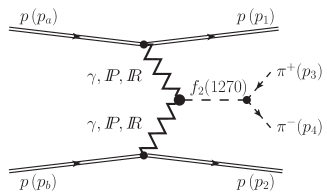
(a) (b)

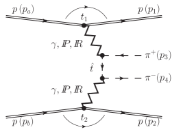
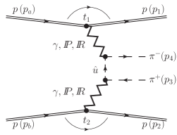
Figure 1: The Born diagrams for the $pp\to pp\pi^{+}\pi^{-}$ reaction. In (a) we have the $\pi^{+}\pi^{-}$ production via the $f_{2}(1270)$ resonance, in (b) the continuum $\pi^{+}\pi^{-}$ production. The exchange objects are the photon ($\gamma$), the pomeron ($\mathbb{P}$) and the reggeons ($\mathbb{R}$).

The kinematic variables for the reaction (1) are

$$s=(p_{a}+p_{b})^{2},\quad s_{34}=M_{\pi\pi}^{2}=(p_{3}+p_{4})^{2},$$

$$q_{1}=p_{a}-p_{1},\quad q_{2}=p_{b}-p_{2},\quad t_{1}=q_{1}^{2},\quad t_{2}=q_{2}^{2},$$

$$p_{34}=q_{1}+q_{2}=p_{3}+p_{4},$$

$$s_{1}=(p_{a}+q_{2})^{2}=(p_{1}+p_{34})^{2},\quad s_{2}=(p_{b}+q_{1})^{2}=(p_{2}+p_{34})^{2}\,.$$ (2)

The $\mathbb{P}\mathbb{P}$-exchange (Born-level) amplitude for $\pi^{+}\pi^{-}$ production via the tensor $f_{2}$-meson ($f_{2}\equiv f_{2}(1270)$) exchange can be written as

$$\begin{split}{\cal M}^{(\mathbb{P}\mathbb{P}\to f_{2}\to\pi^{+}\pi^{-})}_{\lambda_{a}\lambda_{b}\to\lambda_{1}\lambda_{2}\pi^{+}\pi^{-}}=&(-i)\,\bar{u}(p_{1},\lambda_{1})i\Gamma^{(\mathbb{P}pp)}_{\mu_{1}\nu_{1}}(p_{1},p_{a})u(p_{a},\lambda_{a})\;i\Delta^{(\mathbb{P})\,\mu_{1}\nu_{1},\alpha_{1}\beta_{1}}(s_{1},t_{1})\\ &\times i\Gamma^{(\mathbb{P}\mathbb{P}f_{2})}_{\alpha_{1}\beta_{1},\alpha_{2}\beta_{2},\rho\sigma}(q_{1},q_{2})\;i\Delta^{(f_{2})\,\rho\sigma,\alpha\beta}(p_{34})\;i\Gamma^{(f_{2}\pi\pi)}_{\alpha\beta}(p_{3},p_{4})\\ &\times i\Delta^{(\mathbb{P})\,\alpha_{2}\beta_{2},\mu_{2}\nu_{2}}(s_{2},t_{2})\;\bar{u}(p_{2},\lambda_{2})i\Gamma^{(\mathbb{P}pp)}_{\mu_{2}\nu_{2}}(p_{2},p_{b})u(p_{b},\lambda_{b})\,.\end{split}$$ (3)

Here $\Delta^{(\mathbb{P})}$ and $\Gamma^{(\mathbb{P}pp)}$ denote the effective propagator and proton vertex function, respectively, for the tensor-pomeron exchange. For the explicit expressions, see Sect. 3 of Ewerz:2013kda . More details related to the amplitude (3) are given in Lebiedowicz:2016ioh . $\Delta^{(f_{2})}$ and $\Gamma^{(f_{2}\pi\pi)}$ denote the tensor-meson propagator and the $f_{2}\pi\pi$ vertex, respectively. As was mentioned in Ewerz:2013kda we cannot use a simple Breit-Wigner ansatz for the $f_{2}$ propagator in conjunction with the $f_{2}\pi\pi$ vertex from (3.37), (3.38) of Ewerz:2013kda because the partial-wave unitarity relation is not satisfied. We should use, therefore, a model for the $f_{2}$ propagator considered in Eqs. (3.6)–(3.8) and (5.19)–(5.22) of Ewerz:2013kda . The form factor $F^{(f_{2}\pi\pi)}(p_{34}^{2})$ for the $f_{2}\pi\pi$ vertex and for the $f_{2}$ propagator is taken to be the same as (7) below, but with $\Lambda_{f_{2}\pi\pi}$ instead of $\Lambda_{\mathbb{P}\mathbb{P}f_{2}}$.

The main ingredient of the amplitude (3) is the pomeron-pomeron-$f_{2}$ vertex 

$$i\Gamma_{\mu\nu,\kappa\lambda,\rho\sigma}^{(\mathbb{P}\mathbb{P}f_{2})}(q_{1},q_{2})=\left(i\Gamma_{\mu\nu,\kappa\lambda,\rho\sigma}^{(\mathbb{P}\mathbb{P}f_{2})(1)}\mid_{\rm{bare}}+\sum_{j=2}^{7}i\Gamma_{\mu\nu,\kappa\lambda,\rho\sigma}^{(\mathbb{P}\mathbb{P}f_{2})(j)}(q_{1},q_{2})\mid_{\rm{bare}}\right)\tilde{F}^{(\mathbb{P}\mathbb{P}f_{2})}(q_{1}^{2},q_{2}^{2},p_{34}^{2}).\qquad$$ (4)

Here $\tilde{F}^{(\mathbb{P}\mathbb{P}f_{2})}$ is a form factor for which we make a factorised ansatz (see (4.17) of Lebiedowicz:2016ioh )

$$\tilde{F}^{(\mathbb{P}\mathbb{P}f_{2})}(q_{1}^{2},q_{2}^{2},p_{34}^{2})=F_{M}(q_{1}^{2})F_{M}(q_{2}^{2})F^{(\mathbb{P}\mathbb{P}f_{2})}(p_{34}^{2})\,.$$ (5)

We are taking here the same form factor for each vertex with index $j$ ($j=1,...,7$). In principle, we could take a different form factor for each vertex. We take

$$F_{M}(t)=\frac{1}{1-t/\Lambda_{0}^{2}}\,,\quad\Lambda_{0}^{2}=0.5\;{\rm GeV}^{2}\,;$$ (6)

$$F^{(\mathbb{P}\mathbb{P}f_{2})}(p_{34}^{2})=\exp{\left(\frac{-(p_{34}^{2}-m_{f_{2}}^{2})^{2}}{\Lambda_{\mathbb{P}\mathbb{P}f_{2}}^{4}}\right)}\,,\quad\Lambda_{\mathbb{P}\mathbb{P}f_{2}}=1\;{\rm GeV}\,.$$ (7)

The expressions for our bare vertices in (4), obtained from the coupling Lagrangians in Appendix A of Lebiedowicz:2016ioh , are as follows:

$$\begin{split}i\Gamma_{\mu\nu,\kappa\lambda,\rho\sigma}^{(\mathbb{P}\mathbb{P}f_{2})(1)}=2i\,g^{(1)}_{\mathbb{P}\mathbb{P}f_{2}}M_{0}\,R_{\mu\nu\mu_{1}\nu_{1}}\,R_{\kappa\lambda\alpha_{1}\lambda_{1}}\,R_{\rho\sigma\rho_{1}\sigma_{1}}\,g^{\nu_{1}\alpha_{1}}\,g^{\lambda_{1}\rho_{1}}\,g^{\sigma_{1}\mu_{1}}\,,\end{split}$$ (8)

$$\begin{split}i\Gamma_{\mu\nu,\kappa\lambda,\rho\sigma}^{(\mathbb{P}\mathbb{P}f_{2})(2)}(q_{1},q_{2})=-\frac{2i}{M_{0}}\,g^{(2)}_{\mathbb{P}\mathbb{P}f_{2}}\,\Bigl{(}&(q_{1}\cdot q_{2})\,R_{\mu\nu\rho_{1}\alpha}\,R_{\kappa\lambda\sigma_{1}}^{\quad\;\;\,\alpha}-q_{1\rho_{1}}\,q_{2}^{\mu_{1}}\,R_{\mu\nu\mu_{1}\alpha}\,R_{\kappa\lambda\sigma_{1}}^{\quad\;\;\,\alpha}\\ &-q_{1}^{\mu_{1}}\,q_{2\sigma_{1}}\,R_{\mu\nu\rho_{1}\alpha}\,R_{\kappa\lambda\mu_{1}}^{\quad\;\;\,\alpha}+q_{1\rho_{1}}\,q_{2\sigma_{1}}\,R_{\mu\nu\kappa\lambda}\Bigr{)}R_{\rho\sigma}^{\quad\rho_{1}\sigma_{1}}\,,\end{split}$$ (9)

$$\begin{split}i\Gamma_{\mu\nu,\kappa\lambda,\rho\sigma}^{(\mathbb{P}\mathbb{P}f_{2})(3)}(q_{1},q_{2})=-\frac{2i}{M_{0}}\,g^{(3)}_{\mathbb{P}\mathbb{P}f_{2}}\,\Bigl{(}&(q_{1}\cdot q_{2})\,R_{\mu\nu\rho_{1}\alpha}\,R_{\kappa\lambda\sigma_{1}}^{\quad\;\;\,\alpha}+q_{1\rho_{1}}\,q_{2}^{\mu_{1}}\,R_{\mu\nu\mu_{1}\alpha}\,R_{\kappa\lambda\sigma_{1}}^{\quad\;\;\,\alpha}\\ &+q_{1}^{\mu_{1}}\,q_{2\sigma_{1}}\,R_{\mu\nu\rho_{1}\alpha}\,R_{\kappa\lambda\mu_{1}}^{\quad\;\;\,\alpha}+q_{1\rho_{1}}\,q_{2\sigma_{1}}\,R_{\mu\nu\kappa\lambda}\Bigr{)}R_{\rho\sigma}^{\quad\rho_{1}\sigma_{1}}\,,\end{split}$$ (10)

$$\begin{split}i\Gamma_{\mu\nu,\kappa\lambda,\rho\sigma}^{(\mathbb{P}\mathbb{P}f_{2})(4)}(q_{1},q_{2})=-\frac{i}{M_{0}}\,g^{(4)}_{\mathbb{P}\mathbb{P}f_{2}}\,\Bigl{(}q_{1}^{\alpha_{1}}\,q_{2}^{\mu_{1}}\,R_{\mu\nu\mu_{1}\nu_{1}}\,R_{\kappa\lambda\alpha_{1}\lambda_{1}}+q_{2}^{\alpha_{1}}\,q_{1}^{\mu_{1}}\,R_{\mu\nu\alpha_{1}\lambda_{1}}\,R_{\kappa\lambda\mu_{1}\nu_{1}}\Bigr{)}R^{\nu_{1}\lambda_{1}}_{\quad\;\;\;\rho\sigma}\,,\end{split}$$ (11)

$$\begin{split}i\Gamma_{\mu\nu,\kappa\lambda,\rho\sigma}^{(\mathbb{P}\mathbb{P}f_{2})(5)}(q_{1},q_{2})=-\frac{2i}{M_{0}^{3}}\,g^{(5)}_{\mathbb{P}\mathbb{P}f_{2}}\,\Bigl{(}&q_{1}^{\mu_{1}}\,q_{2}^{\nu_{1}}\,R_{\mu\nu\nu_{1}\alpha}\,R_{\kappa\lambda\mu_{1}}^{\quad\;\;\,\alpha}+q_{1}^{\nu_{1}}\,q_{2}^{\mu_{1}}\,R_{\mu\nu\mu_{1}\alpha}\,R_{\kappa\lambda\nu_{1}}^{\quad\;\;\,\alpha}\\ &-2(q_{1}\cdot q_{2})\,R_{\mu\nu\kappa\lambda}\Bigr{)}q_{1\alpha_{1}}\,q_{2\lambda_{1}}\,R^{\alpha_{1}\lambda_{1}}_{\quad\;\;\;\rho\sigma}\,,\end{split}$$ (12)

$$\begin{split}i\Gamma_{\mu\nu,\kappa\lambda,\rho\sigma}^{(\mathbb{P}\mathbb{P}f_{2})(6)}(q_{1},q_{2})=\frac{i}{M_{0}^{3}}\,g^{(6)}_{\mathbb{P}\mathbb{P}f_{2}}\,\Bigl{(}&q_{1}^{\alpha_{1}}\,q_{1}^{\lambda_{1}}\,q_{2}^{\mu_{1}}\,q_{2\rho_{1}}\,R_{\mu\nu\mu_{1}\nu_{1}}\,R_{\kappa\lambda\alpha_{1}\lambda_{1}}\\ &+q_{2}^{\alpha_{1}}\,q_{2}^{\lambda_{1}}\,q_{1}^{\mu_{1}}\,q_{1\rho_{1}}\,R_{\mu\nu\alpha_{1}\lambda_{1}}\,R_{\kappa\lambda\mu_{1}\nu_{1}}\Bigr{)}R^{\nu_{1}\rho_{1}}_{\quad\;\;\;\rho\sigma}\,,\end{split}$$ (13)

$$\begin{split}i\Gamma_{\mu\nu,\kappa\lambda,\rho\sigma}^{(\mathbb{P}\mathbb{P}f_{2})(7)}(q_{1},q_{2})=-\frac{2i}{M_{0}^{5}}\,g^{(7)}_{\mathbb{P}\mathbb{P}f_{2}}\,q_{1}^{\rho_{1}}\,q_{1}^{\alpha_{1}}\,q_{1}^{\lambda_{1}}\,q_{2}^{\sigma_{1}}\,q_{2}^{\mu_{1}}\,q_{2}^{\nu_{1}}\,R_{\mu\nu\mu_{1}\nu_{1}}\,R_{\kappa\lambda\alpha_{1}\lambda_{1}}\,R_{\rho\sigma\rho_{1}\sigma_{1}}\,,\end{split}$$ (14)

where

$$R_{\mu\nu\kappa\lambda}=\frac{1}{2}g_{\mu\kappa}g_{\nu\lambda}+\frac{1}{2}g_{\mu\lambda}g_{\nu\kappa}-\frac{1}{4}g_{\mu\nu}g_{\kappa\lambda}\,.$$ (15)

In (8) to (14) the Lorentz indices of the pomeron with momentum $q_{1}$ are denoted by $\mu\nu$, of the pomeron with momentum $q_{2}$ by $\kappa\lambda$, and of the $f_{2}$ by $\rho\sigma$. Furthermore, $M_{0}\equiv 1$ GeV and the $g^{(j)}_{\mathbb{P}\mathbb{P}f_{2}}$ ($j=1,...,7$) are dimensionless coupling constants. The values of the coupling constants $g^{(j)}_{\mathbb{P}\mathbb{P}f_{2}}$ are not known and are not easy to be found from first principles of QCD, as they are of nonperturbative origin. At the present stage these coupling constants $g_{\mathbb{P}\mathbb{P}f_{2}}^{(j)}$ should be fitted to experimental data.

Considering the fictitious reaction of two “real tensor pomerons” annihilating to the $f_{2}$ meson, see Appendix A of Lebiedowicz:2016ioh , we find that we can associate the couplings (8)–(14) with the following $(l,S)$ values $(0,2)$, $(2,0)-(2,2)$, $(2,0)+(2,2)$, $(2,4)$, $(4,2)$, $(4,4)$, $(6,4)$, respectively.

To give the full physical amplitudes we should include absorptive corrections to the Born amplitudes. For the details how to include the $pp$-rescattering corrections in the eikonal approximation for the four-body reaction see e.g. Sec. 3.3 of Lebiedowicz:2014bea . Other rescattering corrections, such as possible pion-proton Lebiedowicz:2015eka ; Ryutin:2019khx and pion-pion Lebiedowicz:2011nb interactions in the final state, and also so-called “enhanced” corrections Harland-Lang:2013dia , are neglected in the present calculations. In practice we work with the amplitudes in the high-energy approximation; see Eqs. (3.19)–(3.21) and (4.23) of Lebiedowicz:2016ioh .

We are interested in the angular distribution of the $\pi^{+}$ in the center-of-mass system of the $\pi^{+}\pi^{-}$ pair. Various reference systems are commonly used; see e.g. Bolz:2014mya for a discussion of such systems for the $\gamma p\to\pi^{+}\pi^{-}p$ reaction. For the Collins-Soper system Collins:1977iv ; Soper:1982wc for the reaction (1) we set the unit vectors defining the axes as follows:

$$\begin{split}&\mbox{\boldmath$e$}_{\textbf{3},\,\rm CS}=\frac{\mbox{\boldmath$\hat{p}_{a}$}-\mbox{\boldmath$\hat{p}_{b}$}}{|\mbox{\boldmath$\hat{p}_{a}$}-\mbox{\boldmath$\hat{p}_{b}$}|}\,,\\ &\mbox{\boldmath$e$}_{\textbf{2},\,\rm CS}=\frac{\mbox{\boldmath$\hat{p}_{a}$}\times\mbox{\boldmath$\hat{p}_{b}$}}{|\mbox{\boldmath$\hat{p}_{a}$}\times\mbox{\boldmath$\hat{p}_{b}$}|}\,,\\ &\mbox{\boldmath$e$}_{\textbf{1},\,\rm CS}=\frac{\mbox{\boldmath$\hat{p}_{a}$}+\mbox{\boldmath$\hat{p}_{b}$}}{|\mbox{\boldmath$\hat{p}_{a}$}+\mbox{\boldmath$\hat{p}_{b}$}|}\,.\end{split}$$ (16)

These satisfy the condition $\mbox{\boldmath$e$}_{\textbf{1},\,\rm CS}=\mbox{\boldmath$e$}_{\textbf{2},\,\rm CS}\times\mbox{\boldmath$e$}_{\textbf{3},\,\rm CS}$. Here $\mbox{\boldmath$\hat{p}_{a}$}=\mbox{\boldmath$p_{a}$}/|\mbox{\boldmath$p_{a}$}|$, $\mbox{\boldmath$\hat{p}_{b}$}=\mbox{\boldmath$p_{b}$}/|\mbox{\boldmath$p_{b}$}|$, where $p_{a}$, $p_{b}$ are the three-momenta of the initial protons in the $\pi^{+}\pi^{-}$ rest system. There we have $\mbox{\boldmath$p_{34}$}=0$ and $\mbox{\boldmath$p_{a}$}+\mbox{\boldmath$p_{b}$}=\mbox{\boldmath$p_{1}$}+\mbox{\boldmath$p_{2}$}$. Now we denote by $\theta_{\pi^{+},\,{\rm CS}}$ and $\phi_{\pi^{+},\,{\rm CS}}$ the polar and azimuthal angles of $\hat{p}_{3}$ (the $\pi^{+}$ meson momentum) relative to the coordinate axes (16). We have then e.g.

$$\cos\theta_{\pi^{+},{\,\rm CS}}=\mbox{\boldmath$\hat{p}_{3}$}\cdot\mbox{\boldmath$e$}_{\textbf{3},\,\rm CS}\,,$$ (17)

where $\mbox{\boldmath$\hat{p}_{3}$}=\mbox{\boldmath$p_{3}$}/|\mbox{\boldmath$p_{3}$}|$.

Alternatively, for the experiments that can measure at least one of the outgoing protons, the Gottfried-Jackson (GJ) system could be used as well. For the GJ system Gottfried:1964nx we set

$$\begin{split}&\mbox{\boldmath$e$}_{\textbf{3},\,\rm GJ}=\frac{\mbox{\boldmath$q_{1}$}}{|\mbox{\boldmath$q_{1}$}|}\,,\\ &\mbox{\boldmath$e$}_{\textbf{2},\,\rm GJ}=\frac{\mbox{\boldmath$q$}_{\textbf{1},\,\rm c.m.}\times\mbox{\boldmath$q$}_{\textbf{2},\,\rm c.m.}}{|\mbox{\boldmath$q$}_{\textbf{1},\,\rm c.m.}\times\mbox{\boldmath$q$}_{\textbf{2},\,\rm c.m.}|}\,,\\ &\mbox{\boldmath$e$}_{\textbf{1},\,\rm GJ}=\mbox{\boldmath$e$}_{\textbf{2},\,\rm GJ}\times\mbox{\boldmath$e$}_{\textbf{3},\,\rm GJ}\,.\end{split}$$ (18)

Here $q_{1}$ is the three-momentum of the pomeron (emitted by the proton with positive $p_{z}$) in the $\pi^{+}\pi^{-}$ rest system. The second axis of the GJ coordinate system is fixed by the normal to the production plane ($\mathbb{P}$-$\mathbb{P}$-$\pi^{+}\pi^{-}$ plane) in the $pp$ center-of-mass (c.m.) system. $\mbox{\boldmath$q$}_{\textbf{1},\,\rm c.m.}$ and $\mbox{\boldmath$q$}_{\textbf{2},\,\rm c.m.}$ are three-momenta defined in the $pp$ c.m. frame.

For some further remarks on this GJ system see Appendix A.

Having defined these angles we can now examine the differential cross sections $d^{2}\sigma/(d\cos\theta_{\pi^{+},\,{\rm CS}}\,d\phi_{\pi^{+},\,{\rm CS}})$, $d\sigma/d\cos\theta_{\pi^{+},\,{\rm CS}}$, $d\sigma/d\phi_{\pi^{+},\,{\rm CS}}$, and the corresponding distributions in the GJ system.

III Results

As discussed in the introduction, very good observables which can be used for visualizing the role of the $\mathbb{P}\mathbb{P}f_{2}$ couplings, given by Eqs. (8)–(14) (cf. also Appendix A of Lebiedowicz:2016ioh ), could be the differential cross sections $d\sigma/d\cos\theta_{\pi^{+}}$ and $d\sigma/d\phi_{\pi^{+}}$, both in the CS and the GJ systems of reference; see (16) and (18), respectively. In Figs. 2–5 and 7–10 we show such angular distributions for the $\pi^{+}$ meson in the $\pi^{+}\pi^{-}$ rest frame.

In Fig. 2 we collected angular distributions for all (seven) independent $\mathbb{P}\mathbb{P}f_{2}(1270)$ couplings for $\sqrt{s}=13$ TeV, $p_{t,\pi}>0.1$ GeV and for two different cuts on the pseudorapidities of the pions, $|\eta_{\pi}|<1.0$ (the top panels), and $|\eta_{\pi}|<2.5$ (the bottom panels), that will be measured in the LHC experiments. In Fig. 3 we show results for the STAR experimental conditions with extra cuts on the leading protons, specified in Sikora:2018cyk ,

$$(p_{x,p}+0.3\;{\rm GeV})^{2}+p_{y,p}^{2}<0.25\;{\rm GeV}^{2}\,,$$

$$0.2\;{\rm GeV}<|p_{y,p}|<0.4\;{\rm GeV}\,,\quad p_{x,p}>-0.2\;{\rm GeV}\,.$$ (19)

Quite different distributions are obtained for different couplings. Note that the shape of the angular distributions depends on the coverage in $|\eta_{\pi}|$. From the left top panel in Fig. 2 we see that the condition $|\eta_{\pi}|<1.0$ leads to a reduction of the cross sections mostly at $\cos\theta_{\pi^{+},\,{\rm CS}}\approx\pm 1$ compared to the results with $|\eta_{\pi}|<2.5$ shown in the left bottom panel. To our surprise, particularly interesting are the distributions in azimuthal angle. The distributions for the resonance contribution alone can be approximated as

$$d\sigma/d\phi_{\pi^{+},\,{\rm CS}}\approx A\pm B\cos(n\,\phi_{\pi^{+},\,{\rm CS}})\,,$$ (20)

for $|\cos\theta_{\pi^{+},\,{\rm CS}}|<0.5$ (as will be shown below), where $A$ and $B$ depend on experimental conditions. For most of the couplings $n=2$ but for the $j=2$ coupling it is $n=4$. The reader is asked to note the different number of oscillations for the $j=2$ coupling. The shape of $\phi_{\pi^{+},\,{\rm CS}}$ distributions depends also on the cuts on $|\eta_{\pi}|$. Therefore, we expect these differences to be better visible when one compares the results related to different regions of pion pseudorapidity. Let us note that the LHCb Collaboration can measure $\pi^{+}\pi^{-}$ production for $2.0<\eta_{\pi}<4.5$ Goncerz:2018xcw .

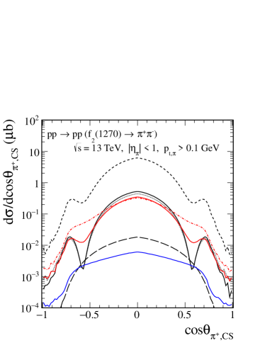
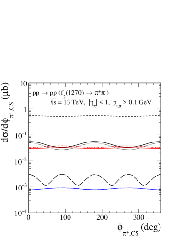
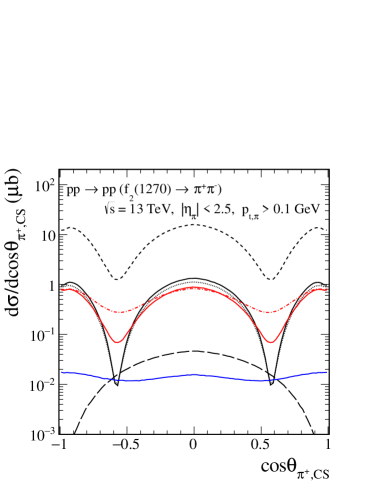
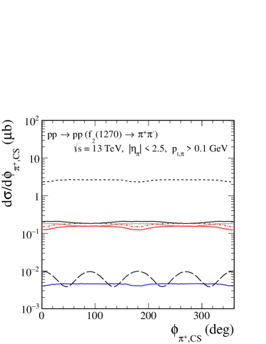
Figure 2: The distributions in $\cos\theta_{\pi^{+},\,{\rm CS}}$ (the left panels) and in $\phi_{\pi^{+},\,{\rm CS}}$ (the right panels) for the $pp\to pp(f_{2}(1270)\to\pi^{+}\pi^{-})$ reaction. The calculations were done for $\sqrt{s}=13$ TeV with different cuts on $|\eta_{\pi}|$ and $p_{t,\pi}>0.1$ GeV. The individual contributions of the different $\mathbb{P}\mathbb{P}f_{2}$ couplings from (8) to (14) are shown: $j=1$ (the black solid line), $j=2$ (the black long-dashed line), $j=3$ (the black dashed line), $j=4$ (the black dotted line), $j=5$ (the blue solid line), $j=6$ (the red solid line), and $j=7$ (the red dot-dashed line). The results correspond to the arbitrary choice of coupling constants $g_{\mathbb{P}\mathbb{P}f_{2}}^{(j)}=1.0$. No absorption effects were included here.

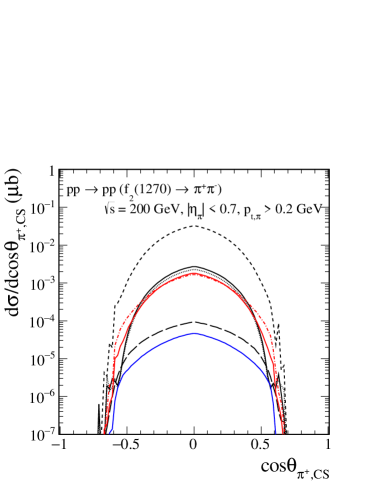
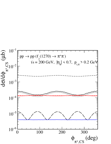
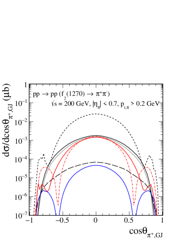
Figure 3: The same as in Fig. 2 but for $\sqrt{s}=200$ GeV and the STAR experimental cuts from Sikora:2018cyk : $|\eta_{\pi}|<0.7$, $p_{t,\pi}>0.2$ GeV, and with cuts on the leading protons (19). In the top panels, we show the pion angular distributions in the $\pi^{+}\pi^{-}$ rest system using the CS frame (16). In the bottom panels, we show the results using the GJ frame (18).

In Fig. 4 we show the two-dimensional distributions in ($\phi_{\pi^{+},\,{\rm CS}},\cos\theta_{\pi^{+},\,{\rm CS}}$) for $\sqrt{s}=13$ TeV and $|\eta_{\pi}|<2.5$. We can observe interesting structures for the $pp\to pp\pi^{+}\pi^{-}$ reaction. We show results for the individual $\mathbb{P}\mathbb{P}f_{2}(1270)$ coupling terms and for the continuum $\pi^{+}\pi^{-}$ production. Different tensorial couplings generate very different patterns which should be checked experimentally.

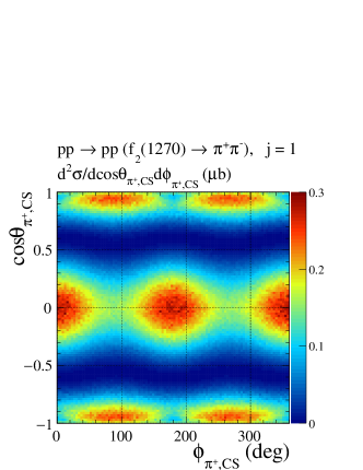
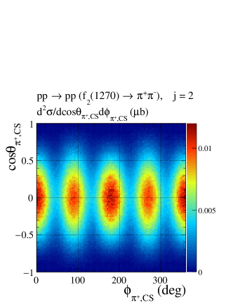
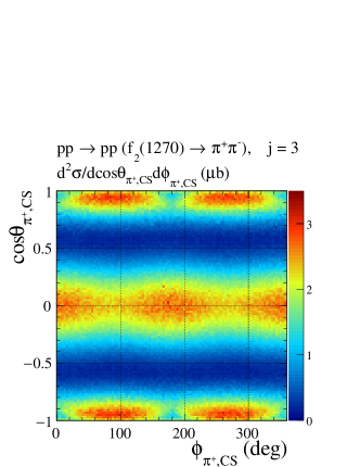
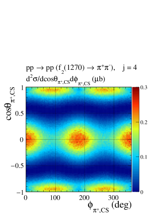
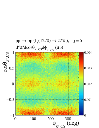
(a) (b) (c) (d) (e) (f)

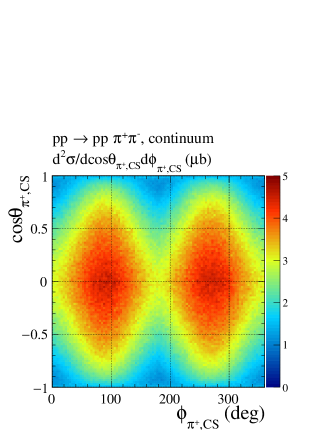
Figure 4: The two-dimensional distributions in ($\phi_{\pi^{+},\,{\rm CS}},\cos\theta_{\pi^{+},\,{\rm CS}}$) for the $pp\to pp\pi^{+}\pi^{-}$ reaction. The calculations were done for $\sqrt{s}=13$ TeV and with cuts on $|\eta_{\pi}|<2.5$. The individual $f_{2}(1270)\to\pi^{+}\pi^{-}$ contributions for five $\mathbb{P}\mathbb{P}f_{2}$ couplings, (a) $j=1$, (b) $j=2$, (c) $j=3$, (d) $j=4$, (e) $j=5$, and (f) the $\pi^{+}\pi^{-}$ continuum term are presented. The results for $\pi^{+}\pi^{-}$ production via $f_{2}(1270)$ resonance were obtained with coupling constants $g_{\mathbb{P}\mathbb{P}f_{2}}^{(j)}=1.0$. No absorption effects were included here.

Some preliminary low-energy COMPASS results Austregesilo:2013yxa ; Austregesilo:2014oxa suggest the presence of two maxima in the $\phi_{\pi^{+},\,{\rm GJ}}$ distribution. So far there are no official analogous data for high-energy scattering either from STAR or the LHC experiments. Nevertheless we have asked ourselves the question if and how we can get a similar structure (two maxima at $\phi_{\pi^{+},\,{\rm GJ}}=\pi/2$, $3/2\pi$) in terms of our $\mathbb{P}\mathbb{P}f_{2}$ couplings (8) to (14).

In Fig. 5 we show the azimuthal angle distributions using the CS (16) and the GJ (18) frames. Here we examine the combination of two $\mathbb{P}\mathbb{P}f_{2}$ couplings: $j=2$ (9) and $j=5$ (12). We show results for the individual $j=2,5$ coupling terms and for their coherent sum. For this purpose, we fixed the $j=2$ coupling constant to $g_{\mathbb{P}\mathbb{P}f_{2}}^{(2)}=1.0$, and assumed various values for $g_{\mathbb{P}\mathbb{P}f_{2}}^{(5)}$. In the top and bottom panels, the red and green lines correspond to the results when both couplings have opposite signs and the same signs, respectively. Different interference patterns can be seen there depending on the ratio of the two couplings, $R=g_{\mathbb{P}\mathbb{P}f_{2}}^{(2)}/g_{\mathbb{P}\mathbb{P}f_{2}}^{(5)}$.

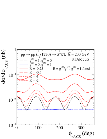
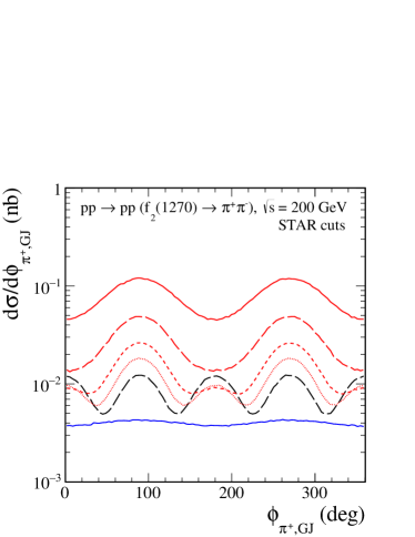
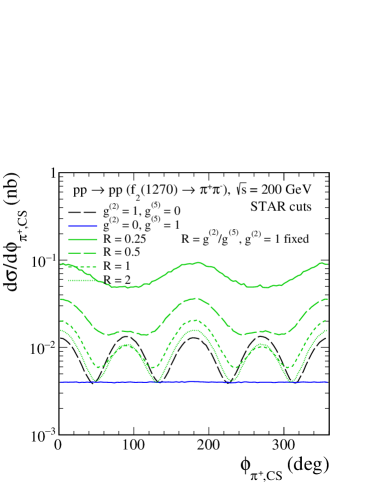
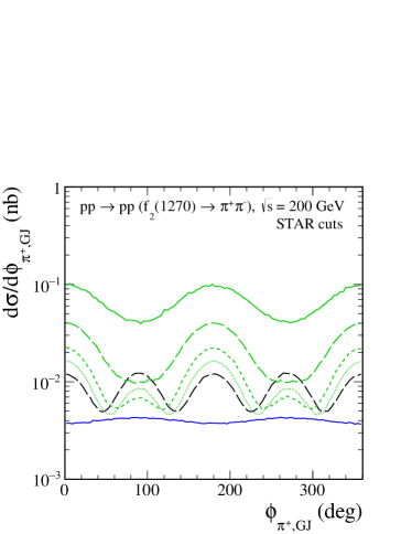
Figure 5: The distributions in azimuthal angle in the $\pi^{+}\pi^{-}$ rest system using the CS frame (left panels) and the GJ frame (right panels), respectively. The calculations were done for the STAR kinematics (see the caption of Fig. 3). No absorption effects were included here.

Now we discuss whether the absorption effects (the $pp$-rescattering corrections) may change the angular distributions discussed so far in the Born approximation. We have checked that a slightly different size of absorption effects may occur for the $j=1,...,7$ resonant terms. The absorption effects lead to a significant reduction of the cross section. However, the shapes of the polar and azimuthal angle distributions are practically not changed. This indicates that the absorption effects should not disturb the determination of the type of the $\mathbb{P}\mathbb{P}f_{2}(1270)$ coupling. However, the continuum and the resonant terms may be differently affected by absorption. This will have to be taken into account when one tries to extract the strengths of the couplings from such distributions.

The measurement of forward protons would be useful to better understand absorption effects. The GenEx Monte Carlo generator Kycia:2014hea ; Kycia:2017ota could be used in this context. We refer the reader to Kycia:2017iij where a first calculation of four-pion continuum production in the $pp\to pp\pi^{+}\pi^{-}\pi^{+}\pi^{-}$ reaction with the help of the GenEx code was performed.

Clearly, by a comparison of our model results to high-energy experimental data we shall be able to determine or at least set limits on the parameters of the $\mathbb{P}\mathbb{P}f_{2}(1270)$ coupling. At the moment, however, this is not yet possible since only some, mostly preliminary, experimental distributions were presented Adamczyk:2014ofa ; Aaltonen:2015uva ; Khachatryan:2017xsi ; Sikora:2018cyk ; CMS:2019qjb .

In Fig. 6 we show the dipion invariant mass distributions for different experimental conditions specified in the legend. One can see the recent high-energy data from the STAR, CDF, and CMS experiments, as well as predictions of our model. Panels (a) and (b) show the preliminary STAR data from Adamczyk:2014ofa and Sikora:2018cyk , respectively. Panels (c) and (d) show the CDF experimental data from Aaltonen:2015uva . Panel (e) shows a very recent result obtained by the CMS Collaboration CMS:2019qjb . In the calculations we include both the nonresonant continuum and $f_{2}(1270)$ terms. The panels (b) and (f) show the results including extra cuts on the outgoing protons. For the STAR experiment we take the cuts (19) and for the ATLAS-ALFA experiment we take 0.17 GeV $<|p_{y,p}|<$ 0.50 GeV. The absorption effects (the $pp$-rescattering corrections only) were taken into account at the amplitude level. The two-pion continuum was fixed by using the monopole form of the off-shell pion form factor with the cut-off parameter $\Lambda_{\rm{off,M}}=0.8$ GeV; see (3.18) of Lebiedowicz:2016ioh . For the $f_{2}(1270)$ contribution, in order to get distinct maxima at $\phi_{\pi^{+},\,{\rm GJ}}=\pi/2$, $3/2\pi$, we take a combination of two $\mathbb{P}\mathbb{P}f_{2}$ couplings, $(g_{\mathbb{P}\mathbb{P}f_{2}}^{(2)},g_{\mathbb{P}\mathbb{P}f_{2}}^{(5)})=(-4.0,16.0)$ (set A) and $(4.0,-16.0)$ (set B), which correspond to the solid and long-dashed lines, respectively. The complete results indicate an interference effect of the continuum and the $f_{2}(1270)$ term. For comparison we show also the contributions of the individual terms separately.

We can see from Fig. 6, that in the $f_{2}$ mass region we describe fairly well the preliminary STAR and CMS data but we overestimate the CDF data Aaltonen:2015uva . In the CMS and CDF measurements there are possible contributions of proton dissociation. The continuum contribution underestimates the data in the region $M_{\pi^{+}\pi^{-}}<1$ GeV, however, there are also possible other processes e.g. from $f_{0}(500)$, $f_{0}(980)$, and $\rho^{0}$ production not included in the present analysis; see e.g. Lebiedowicz:2014bea ; Lebiedowicz:2016ioh . Also other effects, such as the rescattering corrections discussed in Lebiedowicz:2011nb ; Lebiedowicz:2015eka ; Ryutin:2019khx , can be very important there.

We emphasize, that in our calculation of the $\pi^{+}\pi^{-}$-continuum term we include not only the leading pomeron exchanges ($\mathbb{P}\mathbb{P}\to\pi^{+}\pi^{-}$) but also the $\mathbb{P}f_{2\mathbb{R}}$, $f_{2\mathbb{R}}\mathbb{P}$, and $f_{2\mathbb{R}}f_{2\mathbb{R}}$ exchanges. There is interference between the corresponding amplitudes. Their role is very important especially at low energies (COMPASS, WA102, ISR) but even for the STAR kinematics their contribution is not negligible. Adding the $f_{2\mathbb{R}}$ reggeon exchanges increases the cross section by 56% and 45% for the kinematical conditions shown in Figs. 6 (a) and (b), respectively. A similar role of secondary reggeons can be expected for the production of resonances. This means that our results for the $f_{2}(1270)$ resonance (roughly matched to the STAR data) should be treated rather as an upper estimate. This may be the reason why our result for $f_{2}(1270)$ is well above the CDF data.

We summarize this part by the general observation that it is very difficult to describe all available data with the same set of parameters. High-energy central exclusive data expected from CMS-TOTEM and ATLAS-ALFA will allow a better understanding of the diffractive production mechanisms.

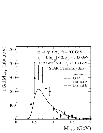
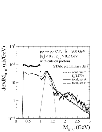
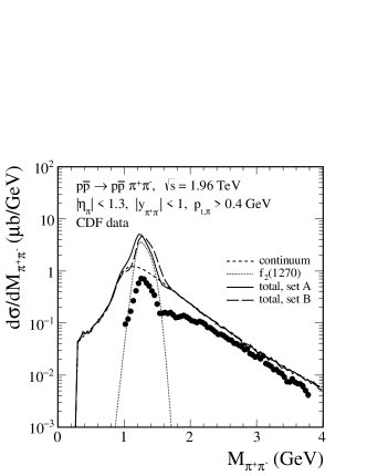
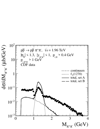
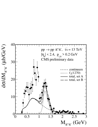
(a) (b) (c) (d) (e) (f)

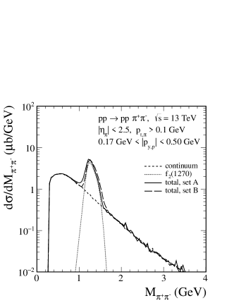
Figure 6: Two-pion invariant mass distributions with the relevant kinematical cuts for (a), (b) STAR, (c), (d) CDF, (e) CMS, and (f) ATLAS-ALFA experiments. The STAR preliminary data from Adamczyk:2014ofa ; Sikora:2018cyk , the CDF data from Aaltonen:2015uva , and the CMS preliminary data from CMS:2019qjb are shown. The calculations for the STAR and ATLAS-ALFA experiments were done with extra cuts on the leading protons. The short-dashed lines represent the nonresonant continuum contribution, the dotted lines represent the results for the $f_{2}(1270)$ contribution, while the solid and long-dashed lines represent their coherent sum for the two parameter sets A and B, respectively. Here we take, in set A $(g_{\mathbb{P}\mathbb{P}f_{2}}^{(2)},g_{\mathbb{P}\mathbb{P}f_{2}}^{(5)})=(-4.0,16.0)$ and, in set B $(g_{\mathbb{P}\mathbb{P}f_{2}}^{(2)},g_{\mathbb{P}\mathbb{P}f_{2}}^{(5)})=(4.0,-16.0)$; see (5), (9), (12). The absorption effects are included here.

In Figs. 7 and 8 we show the two-dimensional angular distributions for the STAR and ATLAS-ALFA kinematics, respectively. In the left panels the results for the CS system and in the right panels for the GJ system are presented. In the top panels we show results for the continuum term, in the center panels for the $f_{2}(1270)$ term, and in the bottom panels for their coherent sum. Here we take the set A with the $\mathbb{P}\mathbb{P}f_{2}$ coupling parameters $(g_{\mathbb{P}\mathbb{P}f_{2}}^{(2)},g_{\mathbb{P}\mathbb{P}f_{2}}^{(5)})=(-4.0,16.0)$. Figures 9 and 10 show that the complete results indicate an interference effect of the continuum and the $f_{2}(1270)$ term calculated for the sets A and B, see the solid and long-dashed lines, respectively. The interference effect depends crucially on the choice of the $\mathbb{P}\mathbb{P}f_{2}(1270)$ coupling. A combined analysis of the $M_{\pi^{+}\pi^{-}}$ and angular distributions in the $\pi^{+}\pi^{-}$ rest frames would, therefore, help to pin down the underlying reaction mechanism.

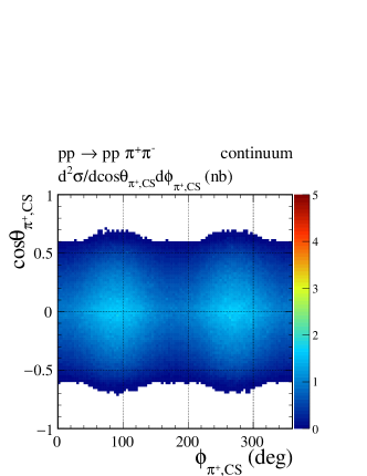
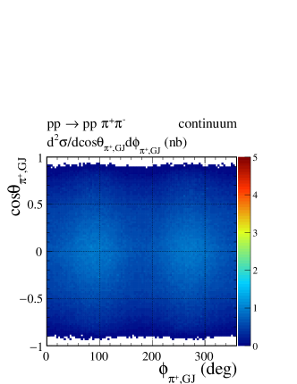
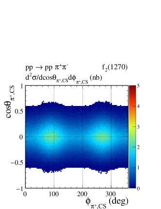
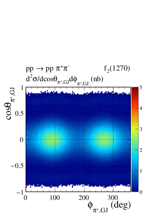
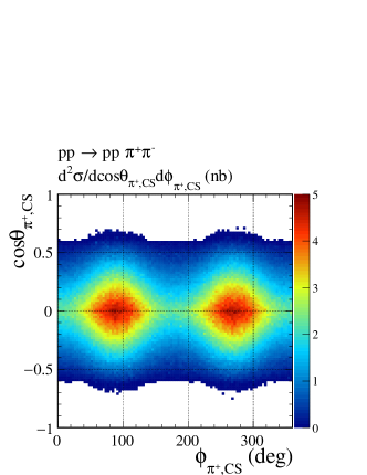
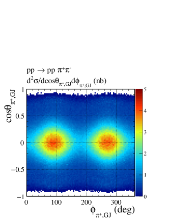
Figure 7: The distributions in ($\phi_{\pi^{+},\,{\rm CS}},\cos\theta_{\pi^{+},\,{\rm CS}}$) (the left panels) and in ($\phi_{\pi^{+},\,{\rm GJ}},\cos\theta_{\pi^{+},\,{\rm GJ}}$) (the right panels) for the $pp\to pp\pi^{+}\pi^{-}$ reaction. The calculations were done in the dipion invariant mass region $M_{\pi^{+}\pi^{-}}\in(1.0,1.5)$ GeV for $\sqrt{s}=200$ GeV and the STAR experimental cuts from Sikora:2018cyk : $|\eta_{\pi}|<0.7$, $p_{t,\pi}>0.15$ GeV, and (19). In the top panels, we show results for the $\pi^{+}\pi^{-}$ continuum term, in the center panels, for the $f_{2}(1270)$ resonance term (set A), and in the bottom panels, for both the contributions added coherently. Here we took $(g_{\mathbb{P}\mathbb{P}f_{2}}^{(2)},g_{\mathbb{P}\mathbb{P}f_{2}}^{(5)})=(-4.0,16.0)$ as discussed in the main text. The absorption effects are included here.

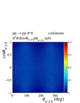
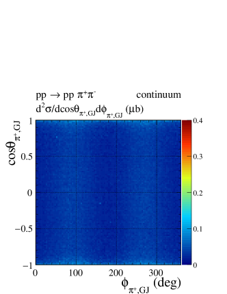
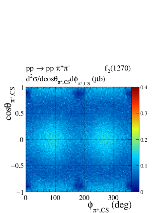
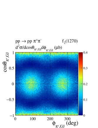
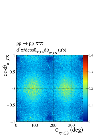
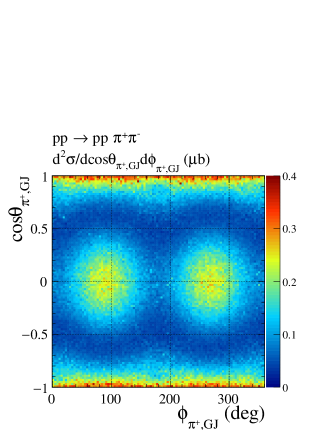
Figure 8: The same as in Fig. 7 but for $\sqrt{s}=13$ TeV and the ATLAS-ALFA experimental cuts: $|\eta_{\pi}|<2.5$, $p_{t,\pi}>0.1$ GeV, and 0.17 GeV $<|p_{y,p}|<$ 0.50 GeV. The calculations were done in the dipion invariant mass region $M_{\pi^{+}\pi^{-}}\in(1.0,1.5)$ GeV. The absorption effects are included here.

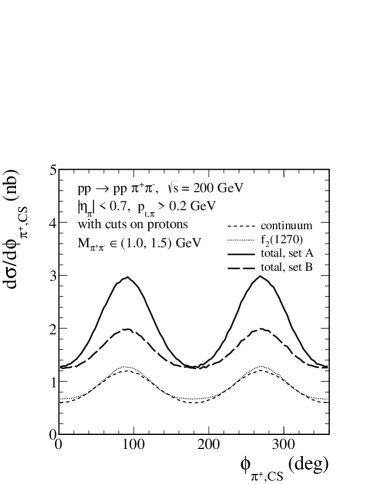
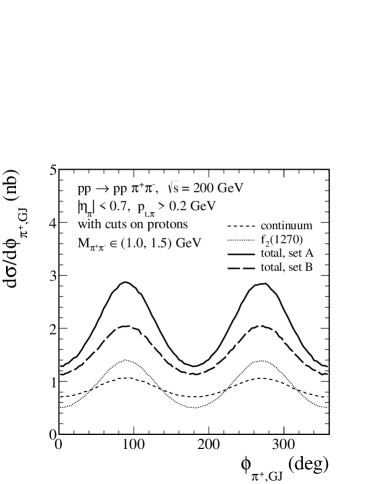
Figure 9: The angular distributions for the $pp\to pp\pi^{+}\pi^{-}$ reaction. The calculations were done for $\sqrt{s}=200$ GeV in the dipion invariant mass region $M_{\pi^{+}\pi^{-}}\in(1.0,1.5)$ GeV and for the STAR experimental cuts specified in Sikora:2018cyk . The results for the $\pi^{+}\pi^{-}$ continuum term (the short-dashed line), for the $f_{2}(1270)$ resonance term (the dotted line), and for their coherent sum (the solid and long-dashed lines corresponding to sets A and B, respectively) are presented. We have taken here A $(g_{\mathbb{P}\mathbb{P}f_{2}}^{(2)},g_{\mathbb{P}\mathbb{P}f_{2}}^{(5)})=(-4.0,16.0)$, and B $(g_{\mathbb{P}\mathbb{P}f_{2}}^{(2)},g_{\mathbb{P}\mathbb{P}f_{2}}^{(5)})=(4.0,-16.0)$ as parameter sets. The absorption effects are included here.

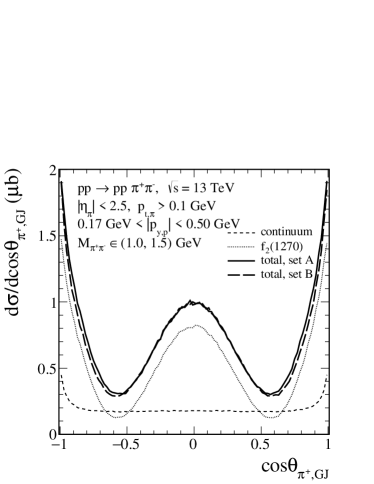
Figure 10: The same as in Fig. 9 but for the ATLAS-ALFA kinematics: $\sqrt{s}=13$ TeV, $|\eta_{\pi}|<2.5$, $p_{t,\pi}>0.1$ GeV, and 0.17 GeV $<|p_{y,p}|<$ 0.50 GeV. The calculations were done in the dipion invariant mass region $M_{\pi^{+}\pi^{-}}\in(1.0,1.5)$ GeV. The absorption effects are included here.

IV Conclusions

In the present work we have considered the possibility to extract the $\mathbb{P}\mathbb{P}f_{2}(1270)$ couplings from the analysis of pion angular distributions in the $\pi^{+}\pi^{-}$ rest system, using the Collins-Soper (CS) and the Gottfried-Jackson (GJ) frames. We have considered the tensor-pomeron model for which there are 7 possible $\mathbb{P}\mathbb{P}f_{2}(1270)$ couplings; see Eqs. (8)–(14) and Appendix A of Lebiedowicz:2016ioh . We have shown that the shape of such distributions strongly depends on the functional form of the $\mathbb{P}\mathbb{P}f_{2}(1270)$ coupling. In particular, we have shown that the azimuthal angle distributions may have different numbers of oscillations. The corresponding distributions can be approximately represented by the formula (20): $A\pm B\cos(n\,\phi_{\pi^{+},\,{\rm CS}})$, where $n=2,4$. Two-dimensional distributions in the CS system ($\phi_{\pi^{+},\,{\rm CS}},\cos\theta_{\pi^{+},\,{\rm CS}}$), ($M_{\pi^{+}\pi^{-}},\phi_{\pi^{+},\,{\rm CS}}$), ($M_{\pi^{+}\pi^{-}},\cos\theta_{\pi^{+},\,{\rm CS}}$), and respectively in the GJ system, will give even more information and could also be useful in understanding the role of experimental cuts. Can such distributions be used to fix the $\mathbb{P}\mathbb{P}f_{2}(1270)$ coupling? The answer will require dedicated experimental studies by the STAR, ALICE, ATLAS-ALFA, CMS-TOTEM, and LHCb Collaborations. This requires comparisons of our model results with precise ’exclusive’ experimental data simultaneously in several differential observables.

We have shown how to select linear combinations of the different $\mathbb{P}\mathbb{P}f_{2}(1270)$ coupling constants to get two maxima in $\phi_{\pi^{+},\,{\rm GJ}}$ (or $\phi_{\pi^{+},\,{\rm CS}}$) as observed at low energies by the COMPASS Collaboration; see Austregesilo:2013yxa ; Austregesilo:2014oxa .

In the diffractive process considered the $f_{2}(1270)$ resonance cannot be completely isolated from the continuum background as the corresponding amplitudes strongly interfere Lebiedowicz:2016ioh . We have discussed how the interference of the resonance and the continuum background may change the angular distributions $d\sigma/d\cos\theta_{\pi^{+},\,{\rm CS}}$ and $d\sigma/d\phi_{\pi^{+},\,{\rm CS}}$. The absorption effects change the overall normalization of such distributions but leave the shape essentially unchanged. This is in contrast to the $d\sigma/d\phi_{pp}$ distributions where absorption effects considerably modify the corresponding shapes; see e.g. Lebiedowicz:2015eka ; Lebiedowicz:2016zka .

In the present analysis we have concentrated on the pronounced $f_{2}(1270)$ resonance, clearly seen in the $\pi^{+}\pi^{-}$ channel. We have discussed methods how to pin down the pomeron-pomeron-$f_{2}(1270)$ coupling. The analysis presented may be extended also to other resonances seen in different final state channels. We strongly encourage experimental groups to start such analyses. We think that this will bring in a new tool for analysing exclusive diffractive processes and will provide new inspirations in searching for more exotic states such as glueballs, for instance. The exclusive diffractive processes were always claimed to be a good area to learn about the physics of glueballs. The extension of our methods to the production of glueballs, to be identified in suitable decay channels, should shed light on the pomeron-pomeron-glueball couplings. These represent very interesting quantities: the coupling of three (mainly) gluonic objects.

Appendix A Remarks on the transformation from the c.m. to the $\pi\pi$ rest system

In this section we discuss the relation between quantities in the c.m. system and the $\pi\pi$ rest system. Momenta in the c.m. system will be denoted by $p_{\rm c.m.}$, $k_{\rm c.m.}$, etc., momenta in the $\pi\pi$ rest system by $p_{\rm R}$, $k_{\rm R}$, etc. We assume that the transformation from the c.m. to the $\pi\pi$ rest system is made by a boost, that is, by a rotation free Lorentz transformation

$$\Lambda(-\mbox{\boldmath$p$}_{\textbf{34},\,\rm c.m.}) = \Bigl{(}\Lambda^{\mu}_{\;\;\;\nu}(-\mbox{\boldmath$p$}_{\textbf{34},\,\rm c.m.})\Bigr{)}$$ (23)

$$= \left(\begin{array}[]{cl}\dfrac{p^{0}_{34,\,\rm c.m.}}{M_{\pi\pi}}&\;\;\dfrac{-p^{j}_{34,\,\rm c.m.}}{M_{\pi\pi}}\\ \dfrac{-p^{i}_{34,\,\rm c.m.}}{M_{\pi\pi}}&\;\;\delta^{ij}+\Bigl{(}\dfrac{p^{0}_{34,\,\rm c.m.}}{M_{\pi\pi}}-1\Bigr{)}\dfrac{p^{i}_{34,\,\rm c.m.}p^{j}_{34,\,\rm c.m.}}{(\mbox{\boldmath$p$}_{\textbf{34},\,\rm c.m.})^{2}}\\ \end{array}\right)\,,$$

where $i,j\in\left\{1,2,3\right\}$.

We have then for any four vector $l=(l^{\mu})$

$$\Lambda(-\mbox{\boldmath$p$}_{\textbf{34},\,\rm c.m.})\,l_{\rm c.m.}=l_{\rm R}\,.$$ (24)

The reverse transformation is $\Lambda^{-1}(-\mbox{\boldmath$p$}_{\textbf{34},\,\rm c.m.})=\Lambda(\mbox{\boldmath$p$}_{\textbf{34},\,\rm c.m.})$

$$\Lambda^{-1}(-\mbox{\boldmath$p$}_{\textbf{34},\,\rm c.m.})\,l_{\rm R}=\Lambda(\mbox{\boldmath$p$}_{\textbf{34},\,\rm c.m.})\,l_{\rm R}=l_{\rm c.m.}\,.$$ (25)

In particular we get

$$\Lambda(-\mbox{\boldmath$p$}_{\textbf{34},\,\rm c.m.})\,p_{34,\,\rm c.m.}=p_{34,\,\rm R}=\left(\begin{array}[]{c}M_{\pi\pi}\\ 0\\ \end{array}\right)\,,$$ (28)

$$\Lambda(-\mbox{\boldmath$p$}_{\textbf{34},\,\rm c.m.})\,\frac{M_{\pi\pi}}{\sqrt{s}}(p_{a}+p_{b})_{\rm c.m.}=\frac{M_{\pi\pi}}{\sqrt{s}}(p_{a}+p_{b})_{\rm R}=\left(\begin{array}[]{c}p^{0}_{34,\,\rm c.m.}\\ -\mbox{\boldmath$p$}_{\textbf{34},\,\rm c.m.}\\ \end{array}\right)\,,$$ (31)

$$q_{1,\,\rm R} = \Lambda(-\mbox{\boldmath$p$}_{\textbf{34},\,\rm c.m.})\,q_{1,\,\rm c.m.}$$ (34)

$$= \left(\begin{array}[]{l}\dfrac{(p_{34}\cdot q_{1})}{M_{\pi\pi}}\\ \mbox{\boldmath$q$}_{\textbf{1},\,\rm c.m.}+\dfrac{\mbox{\boldmath$p$}_{\textbf{34},\,\rm c.m.}}{M_{\pi\pi}}\left(-q^{0}_{1,\,\rm c.m.}+(p^{0}_{34,\,\rm c.m.}-M_{\pi\pi})\dfrac{(\mbox{\boldmath$p$}_{\textbf{34},\,\rm c.m.}\cdot\mbox{\boldmath$q$}_{\textbf{1},\,\rm c.m.})}{(\mbox{\boldmath$p$}_{\textbf{34},\,\rm c.m.})^{2}}\right)\\ \end{array}\right)\,.$$

With these relations we can now express the unit vectors of the Gottfried-Jackson (GJ) system of (18) entirely by vectors defined in the $\pi\pi$ rest system. We have $p_{34}=q_{1}+q_{2}$ and therefore from (31) and (34)

$$\mbox{\boldmath$q$}_{\textbf{1},\,\rm c.m.}\times\mbox{\boldmath$q$}_{\textbf{2},\,\rm c.m.}=\mbox{\boldmath$q$}_{\textbf{1},\,\rm c.m.}\times\mbox{\boldmath$p$}_{\textbf{34},\,\rm c.m.}=-\frac{M_{\pi\pi}}{\sqrt{s}}\mbox{\boldmath$q$}_{\textbf{1},\,\rm R}\times(\mbox{\boldmath$p_{a}$}+\mbox{\boldmath$p_{b}$})_{\rm R}\,;$$ (35)

$$\begin{split}&\mbox{\boldmath$e$}_{\textbf{3},\,\rm GJ}=\frac{\mbox{\boldmath$q$}_{\textbf{1},\,\rm R}}{|\mbox{\boldmath$q$}_{\textbf{1},\,\rm R}|}\,,\\ &\mbox{\boldmath$e$}_{\textbf{2},\,\rm GJ}=-\frac{\mbox{\boldmath$q$}_{\textbf{1},\,\rm R}\times(\mbox{\boldmath$p_{a}$}+\mbox{\boldmath$p_{b}$})_{\rm R}}{|\mbox{\boldmath$q$}_{\textbf{1},\,\rm R}\times(\mbox{\boldmath$p_{a}$}+\mbox{\boldmath$p_{b}$})_{\rm R}|}\,,\\ &\mbox{\boldmath$e$}_{\textbf{1},\,\rm GJ}=\mbox{\boldmath$e$}_{\textbf{2},\,\rm GJ}\times\mbox{\boldmath$e$}_{\textbf{3},\,\rm GJ}\,.\end{split}$$ (36)

Note that for setting up this GJ system only the momentum of one of the outgoing protons in the reaction (1) has to be measured, plus, of course the momenta of $\pi^{+}$ and $\pi^{-}$ giving $p_{34}$.

- (1) C. Ewerz, M. Maniatis, and O. Nachtmann, A Model for Soft High-Energy Scattering: Tensor Pomeron and Vector Odderon, Annals Phys. 342 (2014) 31–77, arXiv:1309.3478 [hep-ph].
- (2) L. Adamczyk et al., (STAR Collaboration), Single spin asymmetry in polarized proton-proton elastic scattering at GeV, Phys. Lett. B719 (2013) 62, arXiv:1206.1928 [nucl-ex].
- (3) C. Ewerz, P. Lebiedowicz, O. Nachtmann, and A. Szczurek, Helicity in Proton-Proton Elastic Scattering and the Spin Structure of the Pomeron, Phys. Lett. B763 (2016) 382, arXiv:1606.08067 [hep-ph].
- (4) D. Britzger, C. Ewerz, S. Glazov, O. Nachtmann, and S. Schmitt, The Tensor Pomeron and Low- Deep Inelastic Scattering, arXiv:1901.08524 [hep-ph]. to be published in Phys. Rev. D.
- (5) P. Lebiedowicz, O. Nachtmann, and A. Szczurek, Exclusive central diffractive production of scalar and pseudoscalar mesons; tensorial vs. vectorial pomeron, Annals Phys. 344 (2014) 301, arXiv:1309.3913 [hep-ph].
- (6) P. Lebiedowicz, O. Nachtmann, and A. Szczurek, and Drell-Söding contributions to central exclusive production of pairs in proton-proton collisions at high energies, Phys. Rev. D91 (2015) 074023, arXiv:1412.3677 [hep-ph].
- (7) P. Lebiedowicz, O. Nachtmann, and A. Szczurek, Central exclusive diffractive production of the continuum, scalar, and tensor resonances in and scattering within the tensor Pomeron approach, Phys. Rev. D93 (2016) 054015, arXiv:1601.04537 [hep-ph].
- (8) P. Lebiedowicz, O. Nachtmann, and A. Szczurek, Central production of in collisions with single proton diffractive dissociation at the LHC, Phys. Rev. D95 no. 3, (2017) 034036, arXiv:1612.06294 [hep-ph].
- (9) P. Lebiedowicz, O. Nachtmann, and A. Szczurek, Towards a complete study of central exclusive production of pairs in proton-proton collisions within the tensor Pomeron approach, Phys. Rev. D98 (2018) 014001, arXiv:1804.04706 [hep-ph].
- (10) P. Lebiedowicz, O. Nachtmann, and A. Szczurek, Exclusive diffractive production of via the intermediate and states in proton-proton collisions within tensor Pomeron approach, Phys. Rev. D94 no. 3, (2016) 034017, arXiv:1606.05126 [hep-ph].
- (11) P. Lebiedowicz, O. Nachtmann, and A. Szczurek, Central exclusive diffractive production of pairs in proton-proton collisions at high energies, Phys. Rev. D97 (2018) 094027, arXiv:1801.03902 [hep-ph].
- (12) P. Lebiedowicz, O. Nachtmann, and A. Szczurek, Central exclusive diffractive production of via the intermediate state in proton-proton collisions, Phys. Rev. D99 no. 9, (2019) 094034, arXiv:1901.11490 [hep-ph].
- (13) P. Lebiedowicz, O. Nachtmann, and A. Szczurek, Searching for the odderon in and reactions in the resonance region at the LHC, arXiv:1911.01909 [hep-ph].
- (14) D. Barberis et al., (WA102 Collaboration), A study of pseudoscalar states produced centrally in interactions at 450 GeV/, Phys.Lett. B427 (1998) 398, arXiv:9803029 [hep-ex].
- (15) D. Barberis et al., (WA102 Collaboration), A coupled channel analysis of the centrally produced and final states in interactions at 450 GeV/, Phys.Lett. B462 (1999) 462, arXiv:9907055 [hep-ex].
- (16) D. Barberis et al., (WA102 Collaboration), Experimental evidence for a vector-like behavior of Pomeron exchange, Phys. Lett. B467 (1999) 165, arXiv:hep-ex/9909013 [hep-ex].
- (17) A. Kirk, Resonance production in central collisions at the CERN Omega Spectrometer, Phys.Lett. B489 (2000) 29, arXiv:0008053 [hep-ph].
- (18) D. Barberis et al., (WA102 Collaboration), A kinematical selection of glueball candidates in central production, Phys.Lett. B397 (1997) 339.
- (19) D. Barberis et al., (WA102 Collaboration), A study of the , , and observed in the centrally produced final states, Phys.Lett. B474 (2000) 423, arXiv:0001017 [hep-ex].
- (20) F. E. Close and A. Kirk, Glueball - filter in central hadron production, Phys.Lett. B397 (1997) 333, arXiv:hep-ph/9701222 [hep-ph].
- (21) A. Breakstone et al., (ABCDHW Collaboration), The reaction Pomeron-Pomeron and an unusual production mechanism for the , Z.Phys. C48 (1990) 569.
- (22) A. Austregesilo, (COMPASS Collaboration), A Partial-Wave Analysis of Centrally Produced Two-Pseudoscalar Final States in Reactions at COMPASS, PoS Bormio2013 (2013) 014.
- (23) A. Austregesilo, Central Production of Two-Pseudoscalar Meson Systems at the COMPASS Experiment at CERN, CERN-THESIS-2014-190.
- (24) A. Austregesilo, (COMPASS Collaboration), Light Scalar Mesons in Central Production at COMPASS, AIP Conf. Proc. 1735 (2016) 030012, arXiv:1602.03991 [hep-ex].
- (25) L. Adamczyk, W. Guryn, and J. Turnau, Central exclusive production at RHIC, Int.J.Mod.Phys. A29 no. 28, (2014) 1446010, arXiv:1410.5752 [hep-ex].
- (26) T. A. Aaltonen et al., (CDF Collaboration), Measurement of central exclusive production in collisions at and 1.96 TeV at CDF, Phys. Rev. D91 (2015) 091101, arXiv:1502.01391 [hep-ex].
- (27) V. Khachatryan et al., (CMS Collaboration), Exclusive and semi-exclusive production in proton-proton collisions at = 7 TeV, CMS-FSQ-12-004, CERN-EP-2016-261, arXiv:1706.08310 [hep-ex].
- (28) R. Sikora, (STAR Collaboration), Recent results on Central Exclusive Production with the STAR detector at RHIC, arXiv:1811.03315 [hep-ex].
- (29) (CMS Collaboration), Measurement of total and differential cross sections of central exclusive production in proton-proton collisions at 5.02 and 13 TeV, CMS-PAS-FSQ-16-006.
- (30) R. Schicker, (ALICE Collaboration), Central exclusive meson production in proton-proton collisions in ALICE at the LHC, arXiv:1912.00611 [hep-ph].
- (31) P. Lebiedowicz and A. Szczurek, Revised model of absorption corrections for the process, Phys. Rev. D92 (2015) 054001, arXiv:1504.07560 [hep-ph].
- (32) R. A. Ryutin, Central exclusive diffractive production of two-pion continuum at hadron colliders, arXiv:1910.06683 [hep-ph].
- (33) P. Lebiedowicz, R. Pasechnik, and A. Szczurek, Measurement of exclusive production of scalar meson in proton-(anti)proton collisions via decay, Phys.Lett. B701 (2011) 434, arXiv:1103.5642 [hep-ph].
- (34) L. A. Harland-Lang, V. A. Khoze, and M. G. Ryskin, Modelling exclusive meson pair production at hadron colliders, Eur.Phys.J. C74 (2014) 2848, arXiv:1312.4553 [hep-ph].
- (35) A. Bolz, C. Ewerz, M. Maniatis, O. Nachtmann, M. Sauter, and A. Schöning, Photoproduction of pairs in a model with tensor-pomeron and vector-odderon exchange, JHEP 1501 (2015) 151, arXiv:1409.8483 [hep-ph].
- (36) J. C. Collins and D. E. Soper, Angular distribution of dileptons in high-energy hadron collisions, Phys. Rev. D16 (1977) 2219.
- (37) D. E. Soper, Angular Distribution of Two Observed Hadrons in Electron-Positron Annihilation, Z. Phys. C17 (1983) 367.
- (38) K. Gottfried and J. D. Jackson, On the Connection between Production Mechanism and Decay of Resonances at High Energies, Nuovo Cim. 33 (1964) 309.
- (39) M. Goncerz, B. Rachwał, and T. Szumlak, (LHCb Collaboration), Central Exclusive Production Measurements in the LHCb, Acta Phys. Polon. B49 (2018) 1135.
- (40) R. A. Kycia, J. Chwastowski, R. Staszewski, and J. Turnau, GenEx: A simple generator structure for exclusive processes in high energy collisions, Commun. Comput. Phys. 24 no. 3, (2018) 860, arXiv:1411.6035 [hep-ph].
- (41) R. A. Kycia, J. Turnau, J. J. Chwastowski, R. Staszewski, and M. Trzebiński, The adaptive Monte Carlo toolbox for phase space integration and generation, Commun. Comput. Phys. 25 no. 5, (2019) 1547, arXiv:1711.06087 [hep-ph].
- (42) R. Kycia, P. Lebiedowicz, A. Szczurek, and J. Turnau, Triple Regge exchange mechanisms of four-pion continuum production in the reaction, Phys. Rev. D95 no. 9, (2017) 094020, arXiv:1702.07572 [hep-ph].