Star Formation Rates of Massive Molecular Clouds in the Central Molecular Zone

Abstract

We investigate star formation at very early evolutionary phases in five massive clouds in the inner 500 pc of the Galaxy, the Central Molecular Zone. Using interferometer observations of H₂O masers and ultra-compact H ii regions, we find evidence of ongoing star formation embedded in cores of 0.2 pc scales and $\gtrsim$10⁵ cm^-3 densities. Among the five clouds, Sgr C possesses a high (9%) fraction of gas mass in gravitationally bound and/or protostellar cores, and follows the dense ($\gtrsim$10⁴ cm^-3) gas star formation relation that is extrapolated from nearby clouds. The other four clouds have less than 1% of their cloud masses in gravitationally bound and/or protostellar cores, and star formation rates 10 times lower than predicted by the dense gas star formation relation. At the spatial scale of these cores, the star formation efficiency is comparable to that in Galactic disk sources. We suggest that the overall inactive star formation in these Central Molecular Zone clouds could be because there is much less gas confined in gravitationally bound cores, which may be a result of the strong turbulence in this region and/or the very early evolutionary stage of the clouds when collapse has only recently started.

1 INTRODUCTION

The classic Kennicutt-Schmidt relation (Schmidt, 1959; Kennicutt, 1998) describes a correlation between the star formation rate (SFR) per unit area and the total gas mass (including both molecular and atomic gases) in galaxies. One of its variations is a linear correlation between the SFR (traced by infrared luminosities or young stellar object counts) and the amount of dense ($\gtrsim$10⁴ cm^-3) molecular gas found in both Galactic sources and external galaxies (Gao & Solomon, 2004; Wu et al., 2005, 2010; Lada et al., 2010, 2012; Zhang et al., 2014), sometimes referred to as the dense gas star formation relation. This linear correlation is suggested to be a result of constant star formation efficiency (SFE) in molecular gas of densities $\gtrsim$10⁴ cm^-3 (Lada et al., 2012).

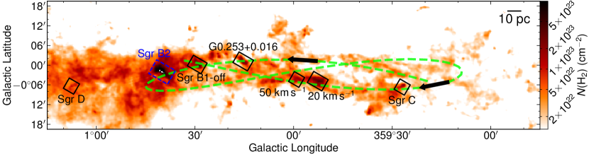
Figure 1: An overview of the CMZ and the six clouds in our observations. The background image shows column densities derived from Herschel data (Battersby et al., 2011). The black boxes mark the same areas toward the six clouds in Figure 2. Sgr B2 is not included in our observations but is discussed in Sections 4.2 & 4.3, and is marked by a blue box. The orbital model for the gas streams in the CMZ proposed by Kruijssen et al. (2015) is shown by the green dashed curve, with two black arrows indicating the direction of the proposed orbital motion.

The Central Molecular Zone (CMZ; Figure 1), the inner 500 pc of our Galaxy, does not fit into this correlation. It contains molecular gas of several times 10⁷ $M_{\odot}$ with mean densities of $\sim$10⁴ cm^-3 (Morris & Serabyn 1996; Ferrière et al. 2007; potential multiple density components from 10³ to 10⁷ cm^-3, Walmsley et al. 1986; Mills et al. 2018), but the SFR is lower by at least an order of magnitude than expected from the dense gas star formation relation, both on the scale of the entire CMZ (e.g., Yusef-Zadeh et al., 2009; An et al., 2011; Immer et al., 2012; Longmore et al., 2013a; Barnes et al., 2017) and of individual clouds (e.g., Kauffmann et al., 2013, 2017a; Barnes et al., 2017). Kauffmann et al. (2017a, b) studied star formation and dense gas content of several representative massive clouds in the CMZ, and concluded that star formation in a time scale of 1.1 Myr in some of the CMZ clouds is $\gtrsim$10 times lower than expected from the linear correlation of Lada et al. (2010).

A possible explanation for the low SFR in the CMZ clouds is that these clouds are at very early evolutionary phases and active star formation has not emerged yet (Kruijssen et al., 2014; Krumholz & Kruijssen, 2015; Krumholz et al., 2017), although this may not be able to account for individual clouds that already show signatures of late evolutionary phases (e.g., H ii regions in several clouds; Kauffmann et al., 2017a). Previous studies using infrared luminosities (e.g., Barnes et al., 2017) or free-free emission from H ii regions (e.g., Longmore et al., 2013a; Kauffmann et al., 2017a) generally characterize star formation in a time scale of a few Myr. A very young generation of star formation deeply embedded in dense gas that is invisible in infrared or free-free emission could have been missed. This young generation of star formation can be traced by masers, ultra-compact (UC) H ii regions, and hot molecular cores that are usually associated with star formation that occurred in the last $<$1 Myr.

Another compelling reason to investigate star formation at very early evolutionary phases is the evolutionary cycling—that is, the potential time delay between the star formation indicated by observations and the observed gas (Kruijssen & Longmore, 2014). The turbulent crossing time scale of the CMZ clouds is $\gtrsim$0.3 Myr (Kruijssen et al., 2014; Federrath et al., 2016; Kauffmann et al., 2013, 2017a). Over a time scale of longer than this, the feedback from star formation may have altered the environment therefore the observed gas reservoir is not directly related to the observed star formation. Such disconnection between active star formation revealed by H ii regions and a lack of dense and massive clumps has been noted for the 50 km s^-1 cloud (Kauffmann et al., 2017b). If we only consider the protostellar population formed in the last 0.3 Myr (i.e., those formed within a time scale comparable to the crossing time), then the derived SFR should be more relevant to the observed gas, although the ratio between star formation and gas is still time-dependent and evolutionary cycling matters.

To investigate star formation at very early evolutionary phases in the CMZ clouds, we conducted observations using the Submillimeter Array (SMA) at 1.3 mm and the Karl J. Jansky Very Large Array (VLA) at the $K$-band toward a sample of six massive clouds (Figures 1 & 2): the 20 km s^-1 cloud, the 50 km s^-1 cloud, G0.253+0.016, Sgr B1-off (also known as Dust Ridge clouds e/f), Sgr C, and Sgr D. This sample has been studied with the SMA at 280 GHz in Kauffmann et al. (2017a, b). Five of them have high column densities ($>$10²³ cm^-2; Figures 1 & 2) and therefore are potential sites of star formation. One cloud, Sgr D, which is associated with an H ii region in projection, has been suggested to reside outside of the CMZ (e.g., Sawada et al., 2009; Sakai et al., 2017). We include it here as a control object. In addition, Sgr B2 is one of the most active star forming regions in the Galaxy and one that we cannot overlook in the CMZ, therefore we compile published data from the literature and include it in the discussion of star formation. Throughout this paper, we adopt a distance of 8.1 kpc (the best-fit distance to Sgr A* in Gravity Collaboration et al., 2018), except for Sgr D, which we adopt 2.36 kpc (the parallax distance from Sakai et al., 2017).

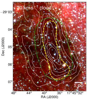
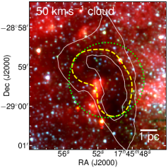
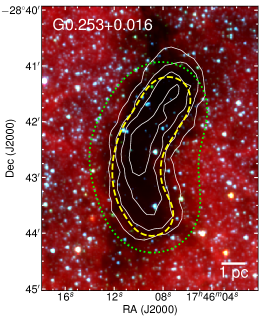
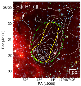
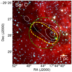
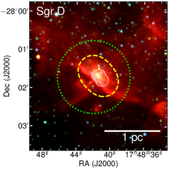
Figure 2: The six clouds in the sample. Background three-color images show Spitzer 3.6 µm (blue), 4.5 µm (green), and 8.0 µm (red) emission. Contours show column densities derived from Herschel data (Battersby et al., 2011), starting from 10²³ cm^-2 in steps of 0.5$\times$10²³ cm^-2. The yellow dashed and green dotted loops in each panel show the mosaic fields of the SMA and VLA, respectively.

In Section 2, we introduce details of the SMA and VLA observations and data reduction. In Section 3, we present the SMA 1.3 mm continuum emission, based on which we identify cores at the 0.2 pc scale and estimate virial states of the cores. We also present VLA $K$-band radio continuum emission and H₂O masers. Then in Section 4, we search for signatures of early phase star formation embedded in the cores using H₂O masers and UC H ii regions. We then estimate SFRs of the clouds in Section 4.2, and compare with the dense gas star formation relation in Section 4.3. The conclusions are in Section 5. All the scripts used in the analyses in this paper are available at https://github.com/xinglunju/CMZclouds.

Table 1: Summary of the SMA and VLA observations.

Project ID / PI	Config.	# of unflagged	Date	Targets	# of	Calibrators
		antennas			pointings	Bandpass	Flux	Gain
SMA 1.3 mm
2012B-S097 / Q. Zhang	SUBCOM	5	2013 May 21	20 km s-1, Sgr C	8+3	Q1	Titan, Neptune	Q2, Q3
	SUBCOM	5	2013 Aug 23	50 km s-1, Sgr B1-off	4+6	Q1, Q4	Neptune	Q2, Q3
2013A-S049 / X. Lu	COM	6	2013 Jul 24	20 km s-1	8	Q1, Q5	Neptune	Q2, Q3
	COM	6	2013 Jul 25	50 km s-1, Sgr C	4+3	Q1	Neptune	Q2, Q3
	COM	6	2013 Aug 01	Sgr B1-off, Sgr D	6+2	Q1	Neptune	Q2, Q3
	COM	6	2013 Aug 02	Sgr B1-off, Sgr D	6+2	Q1	MWC349A	Q2, Q3
	COM	5	2013 Aug 03	20 km s-1	8	Q1, Q5	Neptune	Q2, Q3
	COM	5	2013 Aug 09	20 km s-1	8	Q1, Q6	Neptune	Q2, Q3
2013B-S083 / X. Lu	SUBCOM	7	2014 Mar 10	G0.253+0.016, Sgr D	6+2	Q1	Titan	Q2
	SUBCOM	7	2014 Mar 21	G0.253+0.016, Sgr D	6+2	Q1	Titan	Q2
SMA 1.3 mm archival
2012A-S024 / K. G. Johnston	COM	7	2012 Jun 09	G0.253+0.016	6	Q1	Titan	Q2
VLA K-band
AZ216 / Q. Zhang	DnC	23	2013 May 11	G0.253+0.016, Sgr B1-off	3+2	Q1	Q7	Q3
	DnC	23	2013 May 12	20 km s-1, 50 km s-1	3+1	Q1	Q7	Q3
	DnC	22	2013 May 24	Sgr C, Sgr D	1+1	Q1	Q7	Q3

2 OBSERVATIONS AND DATA REDUCTION

2.1 SMA Observations

The six clouds were observed with the SMA (Ho et al., 2004) in the compact and subcompact array configurations to obtain the 1.3 mm continuum and spectral lines (expect G0.253+0.016 in the compact array configuration, for which we used the archival data). Each cloud was mosaiced with two to eight pointings to cover dense regions seen in the column density maps (see dashed loops in Figure 2). The ASIC correlator was configured to cover 217–221 GHz in the lower sideband and 229–233 GHz in the upper sideband, with a uniform channel width of 0.812 MHz (1.1 km s^-1 at 1.3 mm). Part of the SMA observations toward the 20 km s^-1 cloud has been published in Lu et al. (2015, 2017). Details of the observations are listed in Table 1.

In addition, we obtained the archival SMA 1.3 mm data in the compact array configuration toward G0.253+0.016 (PI: K. G. Johnston), which have been published in Johnston et al. (2014).

The data from the two array configurations were calibrated using the IDL superset MIR. Continuum visibility models were fit using line-free channels with MIRIAD (Sault et al., 1995). Then the two datasets were combined and imaged to produce continuum maps with CASA 4.2.0 (McMullin et al., 2007). Spectral lines were split from the continuum-subtracted visibility data and were imaged separately with a uniform channel width of 1.1 km s^-1. For all images, we used the Briggs weighting with a robustness of 0.5. We did not use multiscale CLEAN or combine with single-dish data, as in our previous work (Lu et al., 2017), because in this paper we intended to study compact cores; therefore, we do not need information on extended structures.

The achieved rms and synthesized beam sizes are summarized in Table 2. The typical synthesized beam size (angular resolution) of continuum images is 5″$\times$3″ (equivalent to 0.2 pc$\times$0.12 pc at the distance of 8.1 kpc), and the typical rms is 3 mJy beam^-1. The continuum images and selected spectral line images are publicly available athttps://doi.org/10.5281/zenodo.1436909 (catalog https://doi.org/10.5281/zenodo.1436909).

The images presented in figures throughout this paper are without primary beam corrections. These images have uniform rms levels across maps and are good for presentation, but the fluxes are attenuated toward the edge of the images. Therefore, when calculating densities and masses (e.g., in Section 3.1), we applied primary beam corrections to the images to have correct fluxes.

Table 2: Properties of the SMA/VLA images.

	Continuum				Spectral lines
Images	Bandwidth	Beam size & PA	RMS		Channel width	Beam size & PA	RMS
	(GHz)	(″$\times$″, °)	(mJy beam-1)		(km s-1)	(″$\times$″, °)	(mJy beam-1)
SMA 1.3 mm
20 km s-1	8	4.9$\times$2.8, 5.2	3		1.1	5.1$\times$2.8, 3.8	110
50 km s-1	8	5.2$\times$2.9, 0.3	3		1.1	5.5$\times$3.2, 1.5	110
G0.253+0.016	8	4.8$\times$3.3, 10.9	2		1.1	5.6$\times$3.8, $-$13.6	60
Sgr B1-off	8	5.2$\times$2.8, $-$9.6	3		1.1	5.6$\times$2.9, $-$8.4	120
Sgr C	8	5.2$\times$2.9, 5.2	3		1.1	5.4$\times$3.1, 5.0	120
Sgr D	8	6.8$\times$4.4, 26.5	4		1.1	7.2$\times$4.6, 26.1	70
VLA K-band
20 km s-1	1	3.1$\times$2.1, 8.5	0.1		0.2	3.5$\times$2.4, 5.5	5.5
50 km s-1	1	2.8$\times$2.2, $-$0.3	0.07		0.2	3.6$\times$2.4, $-$3.6	5.0
G0.253+0.016	1	2.5$\times$2.0, 67.9	0.05		0.2	2.8$\times$2.2, 67.5	4.8
Sgr B1-off	1	2.4$\times$2.0, $-$74.9	0.035		0.2	2.8$\times$2.2, $-$79.4	4.5
Sgr C	1	2.8$\times$2.1, $-$51.8	0.05		0.2	3.1$\times$2.4, $-$54.8	4.5
Sgr D	1	2.5$\times$2.2, $-$61.2	0.2		0.2	2.9$\times$2.3, $-$67.8	4.2

Note. — Beams and rms of the SMA spectral line images are measured for line-free channels of SiO 5–4 images not corrected for primary beam response, but they slightly vary between different lines. Beams and rms of the VLA spectral line images are measured for line-free channels of H₂O maser images. The rms of the SMA and VLA continuum images are measured in emission-free regions away from the emission peaks not corrected for primary beam response.

2.2 VLA Observations

The sample was observed with the NRAO Karl G. Jansky VLA in the DnC configuration, using a $K$-band setup that covers five metastable NH₃ lines from ($J$, $K$)=(1, 1) to (5, 5), an H₂O maser line at 22.235 GHz, and 1 GHz wide continuum centered at $\sim$23 GHz. Part of the observations toward the 20 km s^-1 cloud has been published in Lu et al. (2015, 2017), and details of the VLA observations can be found in Table 1.

The data were calibrated using CASA 4.3.0. In the 20 km s^-1 cloud, Sgr C, and Sgr D, bright ($>$1 Jy) H₂O masers are detected, so we performed self-calibration with the channel where the peak H₂O maser emission is found. We tried two or three rounds of phase-only self-calibration, until the image rms stopped to improve, and did a final round of phase and amplitude self-calibration. Then we applied the calibration tables to the data and produced images of the H₂O masers (see the next paragraph). We compared fluxes of the masers in the final image with those in the initial image to make sure the amplitude is consistent. The rms of channels with strong maser signals was significantly improved, and the achieved dynamic range is up to $\sim$3000. For Sgr D where strong continuum emission is detected, we also applied the calibration tables from the self-calibration of masers to the continuum data to improve the dynamic range, and verified the amplitude consistency by comparing fluxes in images with and without applying the calibration tables.

The calibrated data were imaged using CASA 4.6.0. For the continuum, we used the multiscale CLEAN algorithm (Cornwell, 2008) to improve the imaging of spatially extended structures (e.g., filaments of $>$1 pc). The resulting continuum maps are still dynamic range limited, especially for that of Sgr D, even after applying calibration tables from the self-calibration of H₂O masers. The typical achieved rms is 5 mJy beam^-1 in 0.2 km s^-1 for the H₂O maser, and 35–200 $\mu$Jy beam^-1 for the continuum depending on the target, with a beam size of 3″$\times$2″, as summarized in Table 2. The continuum and maser images are publicly available athttps://doi.org/10.5281/zenodo.1436909 (catalog https://doi.org/10.5281/zenodo.1436909).

3 RESULTS

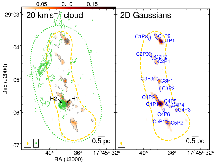
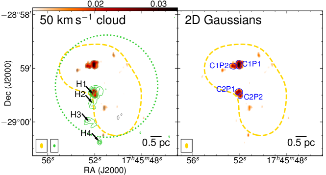
Figure 3: The SMA 1.3 mm continuum and VLA radio continuum emission in the six clouds. On the left side of each panel, both the background image and the grey contours show the SMA 1.3 mm continuum emission, with the scale bar attached to the top in the unit of Jy beam^-1. The contours start at the 5$\sigma$ level and increase in the step of 10$\sigma$, where 1$\sigma$ is 4 mJy beam^-1 for Sgr D, 2 mJy beam^-1 for G0.253+0.016, and 3 mJy beam^-1 for the other four clouds. The green contours show the VLA radio continuum emission, starting at the 5$\sigma$ level in the step of 10$\sigma$ (aside from Sgr D where the step is 20$\sigma$), where 1$\sigma$ values for each map can be found in Table 2. For both the SMA and VLA continuum emissions, dashed contours at the $-$5$\sigma$ level are plotted to show the level of imaging artifacts. (UC) H ii regions identified in Section 3.4 are marked by arrows and labeled. The dashed and dotted loops show the mosaic fields of the SMA and VLA, respectively. The synthesized beams of the SMA and VLA are shown in the bottom left corner. On the right side of each panel, the background image is identical with that on the left side, while the ellipses show the FWHM of 2D Gaussians fit to the cores.

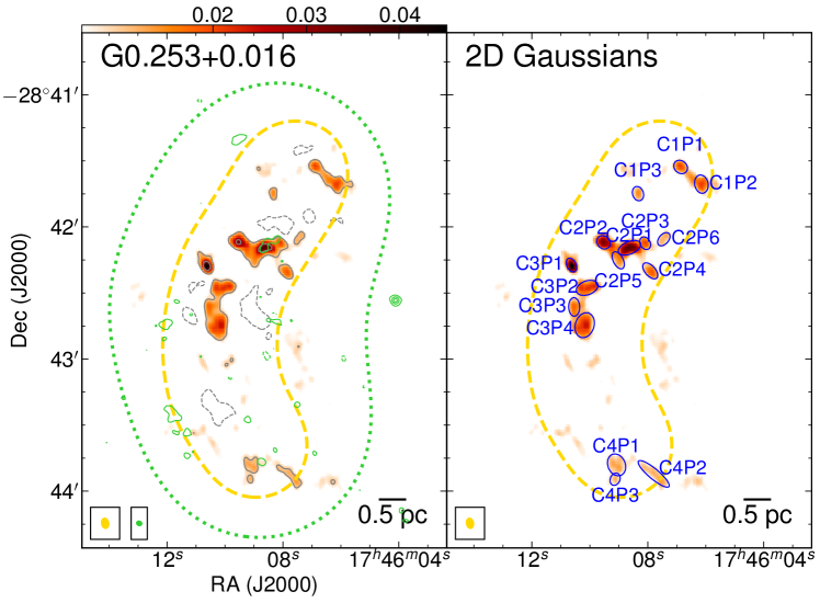
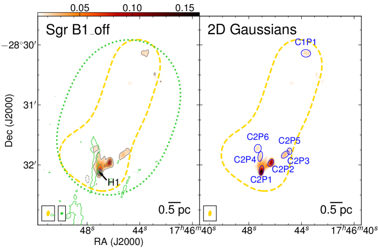
Figure 3: (Continued)

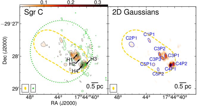
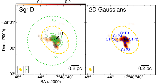
Figure 3: (Continued)

Table 3: Properties of cores.

Core ID	R.A. & Decl.	Deconvl. size & PA	$r_{c}$	Flux	$M_{\text{core}}$	$n$(H2)	$\sigma_{\text{tot}}$	$\alpha_{\text{vir}}$	SF Indicators
	(J2000)	(″$\times$″, °)	(pc)	(mJy)	($M_{\odot}$)	(105 cm-3)	(km s-1)
20 km s-1 C1P1	17:45:37.58, $-$29:03:48.83	7.2$\times$3.2, 48.8	0.09	324	483	20.2	1.27	0.37	W2, W3
C1P2	17:45:38.18, $-$29:03:40.31	11.1$\times$2.8, 28.4	0.11	96	143	3.8	1.29	1.49	W1
C1P3	17:45:39.17, $-$29:03:41.03	12.2$\times$3.3, 5.2	0.12	56	84	1.5	1.83	5.77
C2P1	17:45:38.23, $-$29:04:26.60	10.1$\times$4.1, 36.0	0.13	95	141	2.4	2.51	6.55
C2P2	17:45:38.62, $-$29:04:18.69	9.1$\times$5.0, 22.7	0.13	60	89	1.3	1.44	3.59
C2P3	17:45:39.04, $-$29:04:13.24	7.0$\times$4.0, 34.7	0.10	44	66	2.0	1.13	2.37
C3P1	17:45:37.81, $-$29:05:02.41	6.4$\times$3.1, 178.0	0.09	104	155	8.0	1.93	2.43	W5
C3P2	17:45:37.62, $-$29:05:16.65	9.0$\times$0.5, 3.1	0.04	32	47	22.4	1.39*	2.00	W8
C3P3	17:45:38.28, $-$29:04:58.59	9.0$\times$5.1, 90.8	0.13	56	84	1.2	1.47	3.99
C4P1	17:45:37.64, $-$29:05:43.65	7.8$\times$5.4, 68.0	0.13	468(459)	684	11.4	1.56	0.53	W11–W13, H1
C4P2	17:45:38.23, $-$29:05:32.72	14.0$\times$3.5, 30.5	0.14	196(195)	291	3.9	1.43*	1.12
C4P3	17:45:35.36, $-$29:05:55.53	4.1$\times$1.7, 99.0	0.05	52	78	19.2	1.27	1.25	W16
C4P4	17:45:36.25, $-$29:05:49.03	5.0$\times$2.7, 56.0	0.07	38	57	5.2	2.15	6.83	W15
C4P5	17:45:36.74, $-$29:05:45.93	$<$5.2$\times$3.1, 33.2	$<$0.08	18	26	$>$1.8	1.08	$<$4.12	W14
C4P6	17:45:37.16, $-$29:05:55.13	3.4$\times$2.6, 6.2	0.06	19	28	4.9	1.20	3.42	W17
C5P1	17:45:36.71, $-$29:06:17.50	7.1$\times$3.9, 73.4	0.10	95	142	4.4	1.21	1.25
C5P2	17:45:36.43, $-$29:06:19.55	6.6$\times$4.4, 13.1	0.11	76	113	3.3	1.06	1.22
50 km s-1 C1P1	17:45:52.08, $-$28:58:55.91	4.3$\times$3.1, 0.5	0.07	72	107	10.0	5.17	20.9	W2
C1P2	17:45:52.57, $-$28:58:57.61	4.2$\times$2.2, 81.8	0.06	46	69	11.2	5.21	27.2
G0.253+0.016 C1P1	17:46:06.87, $-$28:41:32.79	5.4$\times$3.7, 72.0	0.09	31	45	2.3	2.35	12.4
C1P2	17:46:06.15, $-$28:41:40.57	7.0$\times$5.2, 12.1	0.12	57	85	1.8	2.35	8.95
C1P3	17:46:08.34, $-$28:41:44.90	4.7$\times$3.7, 27.0	0.08	16	25	1.6	1.39	7.50
C2P1	17:46:08.63, $-$28:42:09.50	10.4$\times$3.2, 111.1	0.11	78(76)	113	2.7	2.61	7.94
C2P2	17:46:09.53, $-$28:42:07.00	5.3$\times$3.7, 74.2	0.09	42	62	3.3	1.24	2.51
C2P3	17:46:08.09, $-$28:42:07.40	4.2$\times$2.6, 55.2	0.06	22	32	4.1	1.48	5.18
C2P4	17:46:07.92, $-$28:42:19.96	7.7$\times$2.8, 48.0	0.09	38	57	2.6	2.62	12.9
C2P5	17:46:09.02, $-$28:42:15.18	7.1$\times$2.9, 32.0	0.09	20	31	1.5	1.86	11.7
C2P6	17:46:07.45, $-$28:42:05.59	$<$7.0$\times$4.4, 139.0	$<$0.11	20	29	$>$0.8	$\cdots$	$\cdots$
C3P1	17:46:10.63, $-$28:42:17.35	4.9$\times$2.5, 36.0	0.07	46	69	7.4	3.24*	12.1	W2
C3P2	17:46:10.09, $-$28:42:27.69	9.7$\times$4.2, 108.5	0.13	51	76	1.3	2.21	9.32
C3P3	17:46:10.54, $-$28:42:36.53	6.8$\times$2.7, 4.4	0.08	23	34	2.0	1.60	7.35
C3P4	17:46:10.18, $-$28:42:44.65	10.8$\times$7.6, 157.6	0.18	79	118	0.7	3.84*	25.9
C4P1	17:46:09.08, $-$28:43:48.09	9.2$\times$7.1, 27.0	0.16	46	69	0.6	1.96	10.2
C4P2	17:46:07.80, $-$28:43:52.17	17.5$\times$2.4, 51.1	0.13	64	95	1.6	1.98	6.15
C4P3	17:46:09.13, $-$28:43:54.60	4.2$\times$1.5, 132.0	0.05	15	22	6.4	2.43	15.1
Sgr B1-off C1P1	17:46:43.66, $-$28:30:08.43	9.2$\times$5.5, 84.0	0.14	71	106	1.3	3.19*	15.6
C2P1	17:46:47.05, $-$28:32:05.50	8.4$\times$3.7, 171.6	0.11	222(221)	329	8.7	0.84	0.27	W5, H1
C2P2	17:46:46.33, $-$28:31:58.00	6.1$\times$3.6, 130.0	0.09	144	215	9.5	1.84	1.68	W3
C2P3	17:46:45.23, $-$28:31:49.62	8.3$\times$3.4, 121.8	0.10	82	123	3.7	1.80	3.20
C2P4	17:46:47.14, $-$28:31:51.49	8.6$\times$3.6, 170.4	0.11	40(39)	58	1.5	2.47	13.3
C2P5	17:46:44.91, $-$28:31:46.36	4.6$\times$3.5, 31.7	0.08	50	74	5.2	$\cdots$	$\cdots$
C2P6	17:46:47.32, $-$28:31:43.63	6.7$\times$6.4, 151.0	0.13	44(41)	61	1.0	1.48	5.39
Sgr C C1P1	17:44:43.58, $-$29:27:30.71	7.3$\times$0.4, 34.0	0.03	54	80	72.8	1.22*	0.73	W2
C2P1	17:44:46.07, $-$29:27:38.18	9.5$\times$6.9, 61.0	0.16	80	119	1.0	0.97	1.46	W3
C3P1	17:44:41.27, $-$29:27:59.38	7.1$\times$2.8, 4.3	0.09	206(205)	306	15.7	1.60	0.86	W8, W9, H1, H2
C3P2	17:44:42.11, $-$29:27:56.96	6.3$\times$2.5, 22.8	0.08	122	183	13.3	1.85*	1.70	W7, W10
C3P3	17:44:41.73, $-$29:28:03.22	7.0$\times$1.4, 51.8	0.06	118	177	26.2	1.39	0.78	W11
C4P1	17:44:40.58, $-$29:28:16.28	4.2$\times$2.8, 144.0	0.07	462(457)	681	77.0	1.80	0.37	W13, H4
C4P2	17:44:40.16, $-$29:28:14.43	4.5$\times$2.9, 160.0	0.07	335(330)	492	47.6	1.70	0.48	W12, H3
C5P1	17:44:42.98, $-$29:28:15.14	4.1$\times$2.2, 99.0	0.06	42	63	10.5	2.19	5.23	W14
C5P2	17:44:42.32, $-$29:28:24.15	3.7$\times$1.7, 16.0	0.05	30	44	12.7	2.31	6.96
Sgr D C1P1	17:48:41.46, $-$28:01:39.74	13.1$\times$8.2, 3.3	0.06	616(152)	15	2.4	0.89	3.74	W3, W4, H1
C1P2	17:48:41.06, $-$28:01:40.22	7.9$\times$4.5, 30.7	0.03	276(144)	14	12.0	1.69	8.23	W5, H1
C1P3	17:48:41.35, $-$28:01:53.67	7.2$\times$2.8, 28.2	0.03	216	21	42.0	2.54	9.30	W7
C1P4	17:48:42.05, $-$28:01:39.36	6.8$\times$3.1, 100.6	0.03	168(95)	9	17.3	1.84	11.4	W4, H1
C1P5	17:48:42.92, $-$28:01:40.20	6.9$\times$4.0, 34.9	0.03	78	8	9.5	1.43*	9.53	W2

Note. — Uncertainties of the core properties are discussed in Section 3.3.

3.1 SMA Dust Emission

The SMA 1.3 mm continuum emission maps of the six clouds are shown in Figure 3. We identified compact structures with peak values above the 5$\sigma$ level and areas larger than the synthesized beams, and within FWHM of the SMA primary beams. Then we fit 2D Gaussians using the interactive tool in CASAviewer to obtain their positions, deconvolved FWHM sizes, and fluxes. To have uniform noise levels so that we can apply the same fitting criteria across the maps, we performed the fit in the images without primary beam corrections. We took the deconvolved FWHM of the 2D Gaussians as the sizes of the compact structures. The fluxes inside the deconvolved FWHM of the 2D Gaussians are half of the measured fluxes of the whole Gaussian profiles, which we took as the fluxes of the compact structures after applying the primary beam correction. In Section 3.1, we derived the mean densities inside the deconvolved FWHM sizes using these fluxes.

The dendrogram algorithm is a widely used method for source identification in radio astronomy (Rosolowsky et al., 2008). We compared our result with the outcome of dendrogram, shown in Appendix A, and found that they are generally consistent. However, dendrogram is not able to separate closely packed structures (e.g., the two emission peaks in the southwestern end of Sgr C). It also misses several compact structures that are slightly smaller than the synthesized beam size but are spatially coincident with H₂O masers and therefore are likely protostellar cores in nature (e.g., in the southern part of the 20 km s^-1 cloud). In light of this, we chose to rely on manual identification and added these structures for consideration.

In the end, we identified 58 structures, marked by ellipses in Figure 3. They are named by the indices of ‘clumps’ they belong to, plus the indices of peaks inside the clumps in decreasing order of peak intensities. Here the clumps do not have physical meanings but are for name tagging.

We stress that the identification of compact structures is unlikely to be complete. Some features, especially those in crowded environments (e.g., the C4 clump in the 20 km s^-1 cloud, the C2 clump in Sgr C), may have been missed. Nevertheless, we intended to study characteristic physical properties of dense gas in these clouds, and structures identified using this approach make up a good sample for our purpose.

At the wavelength of 1.3 mm, the continuum emission in molecular clouds is often attributed to thermal dust emission associated with dense gas (e.g., Beuther et al., 2002), but can also be free-free emission from embedded H ii regions (e.g., Motte et al., 2003). To examine potential contribution from free-free emission, we compared the 1.3 mm continuum with the radio continuum data in Section 3.4. Two compact structures, C2P1 and C2P2 in the 50 km s^-1 cloud, are associated with radio continuum emission of similar or even higher fluxes than the 1.3 mm continuum emission. As discussed in Section 3.4, the radio continuum in the 50 km s^-1 cloud arises from several known H ii regions. The 1.3 mm continuum emission of the two compact structures therefore is likely dominated by free-free emission from the H ii regions. These two structures are excluded from Table 3. A few compact structures in the 20 km s^-1 cloud, Sgr B1-off, Sgr C, and Sgr D are also found to be associated with compact radio continuum emission, which is much weaker than the 1.3 mm continuum emission.

We obtained dust emission fluxes of the compact structures after excluding the contribution from free-free emission in the 1.3 mm continuum emission. We used a flat spectral index from centimeter to 1.3 mm, assuming slightly optically thick thermal free-free emission. If there is any optically thick free-free emission from hyper-compact H ii regions, the spectral index between the frequencies of the VLA and SMA observations may be positive (rising), and the free-free contribution in the 1.3 mm continuum emission will be greater. However, hyper-compact H ii regions are rare (the only known cases in the CMZ are six hyper-compact H ii regions in Sgr B2; De Pree et al., 2015), so we did not consider optically thick free-free emission in our assumption. Then we subtracted the radio continuum fluxes inside the FWHM of the compact structures from the corresponding 1.3 mm continuum fluxes and obtained the dust emission fluxes, which are listed in parentheses in Table 3. Following the nomenclature of Zhang et al. (2009), these structures with typical radii of 0.1 pc are defined as cores. Excluding the two compact structures in the 50 km s^-1 cloud that are dominated by free-free emission, we identified 56 cores in the six clouds, as listed in Table 3.

We derived core masses following

$$M_{\text{core}}=R\frac{S_{\nu}d^{2}}{B_{\nu}(T_{\text{dust}})\kappa_{\nu}},$$ (1)

where $R$ is the gas-to-dust mass ratio, $S_{\nu}$ is the dust emission flux, $d$ is the distance, $B_{\nu}(T_{\text{dust}})$ is the Planck function at the dust temperature $T_{\text{dust}}$, and $\kappa_{\nu}$ is the dust opacity. We assumed $R$=100, and $\kappa_{\nu}$=0.899 cm² g^-1 (MRN model with thin ice mantles, after 10⁵ years of coagulation at 10⁶ cm^-3; Ossenkopf & Henning, 1994). We assumed $T_{\text{dust}}=20$ K for the cores, except for those in Sgr D where $T_{\text{dust}}$ is taken to be 25 K, which are estimated from multi-band SED fitting of Herschel data (Kauffmann et al., 2017a). The masses of the cores are listed in Table 3. With a dust emission rms of 3 mJy beam^-1, the 5$\sigma$ mass sensitivity is 22 $M_{\odot}$ per beam for the CMZ clouds.

Assuming a spherical geometry with a radius $r_{a}$ that is equivalent to half of the geometric mean of the deconvolved angular sizes of the cores, densities of molecular gas in the cores are derived with

$$\begin{split}n(\text{H}_{2})&=\frac{3M_{\text{core}}}{4\pi r_{a}^{3}d^{3}}\frac{1}{2.8m_{\text{H}}}\\ &=R\frac{S_{\nu}}{B_{\nu}(T_{\text{dust}})\kappa_{\nu}}\frac{3}{4\pi r_{a}^{3}d}\frac{1}{2.8m_{\text{H}}},\end{split}$$ (2)

where 2.8 is the molecular weight per H₂ molecule (Kauffmann et al., 2008) and $m_{\text{H}}$ is the mass of a hydrogen atom.

We caution that these cores are defined in terms of their spatial scales, but they are more massive than dense cores in nearby molecular clouds at the same spatial scale (e.g., Alves et al., 2007), and their densities are an order of magnitude higher ($\gtrsim$10⁵ cm^-3 vs. $\sim$10⁴ cm^-3). They may each form a cluster of stars instead of a single star or a multiple star system as assumed for those dense cores in nearby clouds. With higher angular resolutions, they may be further resolved into objects that map to individual protostars (e.g., Ginsburg et al., 2018).

Sgr B1-off is included in the SMA sample of Walker et al. (2018) with a similar observation setup. They identified two cores e1 and e2, corresponding to C2P1 and C2P2 in this cloud in Figure 3 and Table 3. The masses we derived are 40% to 50% smaller than their results, because we only considered fluxes inside the deconvolved FWHM sizes therefore the measured fluxes are smaller. They also estimated densities of these cores to be 10⁵–10⁶ cm^-3, much higher than those of dense cores in nearby clouds.

3.2 Virial States of the Cores

We studied virial states of the cores in these clouds. The virial parameter is defined as (Bertoldi & McKee, 1992)

$$\alpha_{\text{vir}}=\frac{5\sigma_{\text{tot}}^{2}r_{a}d}{\text{G}M_{\text{core}}},$$ (3)

in which $r_{a}$ is the angular radius of the core as defined above, and $\sigma_{\text{tot}}$ is the total one-dimensional line width including both thermal and non-thermal components. The properties can be found in Table 3.

The total line width $\sigma_{\text{tot}}$ was measured with the N₂H⁺ 3–2 line (Kauffmann et al., 2017a), which has a critical density of $\gtrsim$10⁶ cm^-3 at a temperature of $\gtrsim$50 K (Shirley, 2015). In the starless core candidates where gas temperatures are low (see Section 4.1.4), N₂H⁺ may be chemically biased toward denser regions where CO is frozen out onto dust grains, therefore it may preferentially trace smaller line widths from smaller spatial scales (Caselli et al., 2002). When N₂H⁺ is not detected, the CH₃OH line in our SMA 1.3 mm line data (not combined with single-dish data) is used, which has been shown to best spatially correlated with the dust emission among the 1.3 mm molecular lines (Lu et al., 2017). However, CH₃OH is likely influenced by shocks, so we only used it as a second choice. Two cores, C2P6 in G0.253+0.016 and C2P5 in Sgr B1-off, are not detected in N₂H⁺ or CH₃OH lines, therefore their virial parameters cannot be determined. We fit a single Gaussian to the mean spectrum of each core, shown in Appendix C, to obtain the intrinsic line width $\sigma_{v}$ that is deconvolved from the channel width. When both the N₂H⁺ and CH₃OH lines are detected, the line widths measured from them are usually consistent within a factor of 1.5.

Our VLA observations cover five VLA NH₃ lines, but we did not use them to measure line widths of the cores for three reasons. First, for the lower NH₃ transitions, ($J$, $K$)=(1, 1), (2, 2), and (3, 3), the hyperfine components tend to be blended together and strong absorption features are frequently seen toward the cores. Second, for the higher NH₃ transitions, ($J$, $K$)=(4, 4) and (5, 5), the signal-to-noise ratio is much lower (e.g., Figure 15 of Lu et al., 2017). Third, the critical densities of the NH₃ lines are of the order 10³ cm^-3 at a temperature of $\gtrsim$50 K (Shirley, 2015), therefore may not be as good as N₂H⁺ for tracing of gas in the cores. Nonetheless, we attempted to fit the NH₃ spectra when they are optically thin and absorption is not significant (e.g., toward C1P1 in the 20 km s^-1 cloud), and the measured line widths agree with those based on N₂H⁺ within a factor of 1.5.

We assume a gas temperature $T_{\text{gas}}$ of 100 K. This is the typical temperature for cores at 0.2 pc scales based on non-LTE modeling of NH₃ (2, 2) and (4, 4) lines (Lu et al., 2017), and it generally agrees with those in previous observations (Ao et al., 2013; Ginsburg et al., 2016; Krieger et al., 2017). Then we derive the line width $\sigma_{\text{tot}}$:

$$\sigma_{\text{tot}}=\sqrt{\sigma_{v}^{2}-\frac{k_{B}T_{\text{gas}}}{\mu_{m}m_{p}}+\frac{k_{B}T_{\text{gas}}}{\mu_{p}m_{p}}},$$ (4)

in which the mean molecule weight $\mu_{p}$ is 2.33, assuming 90% H and 10% He, and $\mu_{m}$ is 29 or 32 (i.e., the molecule weight of N₂H⁺ or CH₃OH, depending on which line is used to measure the linewidth).

The derived virial parameters $\alpha_{\text{vir}}$ are listed in Table 3. Out of the 54 cores whose virial parameters can be determined, 17 have $\alpha_{\text{vir}}\leq 2$. These cores are likely gravitationally bound and unstable to collapse.

Table 4: Summary of uncertainties in derived core properties.

Core properties	Related equations	Considered quantities and random errors	Uncertainties
Mass ($M_{\text{core}}$)	Equation 1	$\kappa_{\nu}$ (28%), $S_{\nu}$ (15%), $d$ (1.2%), $R$ (50%)	59%
Density ($n$(H2))	Equation 2	$\kappa_{\nu}$ (28%), $S_{\nu}$ (15%), $d$ (1.2%), $R$ (50%), $r_{a}$ (10%)	66%
Virial parameter ($\alpha_{\text{vir}}$)	Equation 3	$\kappa_{\nu}$ (28%), $S_{\nu}$ (15%), $d$ (1.2%), $R$ (50%), $r_{a}$ (10%), $\sigma_{\text{tot}}$ (50%)	120%

3.3 Uncertainties of Core Properties

We reported uncertainties in the derived masses, densities, line widths, and virial parameters of the cores. The uncertainties are summarized in Table 4.

The derived core masses depend on the dust opacity, the gas-to-dust mass ratio, dust temperatures, dust emission fluxes, and distances. We followed Sanhueza et al. (2017) to adopt uncertainties of 28% and 15% for the dust opacity and measured dust emission fluxes at 1.3 mm. The uncertainty in the distance to Sgr A* is small (0.4%; Gravity Collaboration et al., 2018). However, given that the clouds may be on an orbit of radius$\sim$100 pc around Sgr A* (Molinari et al., 2011; Kruijssen et al., 2015), we adopt an uncertainty of $\pm$100 pc (1.2%) for the distance.

The gas-to-dust mass ratio has a large uncertainty. The value of 100 adopted for Equation 1 is characteristic for nearby clouds, although values up to 150 have been suggested (Draine, 2011). On the other hand, the value for Galactic Center regions may be as low as $\sim$50 (Giannetti et al., 2017). Therefore, the uncertainty in the gas-to-dust ratio is adopted to be 50%.

The dust temperature may have a large systematic error for the cores that are internally heated by protostars. It could reach 50 K around hot molecular cores at the radius of 0.1 pc (Longmore et al., 2011), in which case the derived core masses using Equation 1 would decrease by a factor of 3. This only affects cores with significant internal heating (potentially those with star formation indicators in Table 3), and may not be an issue for cores without signatures of star formation. Further discussion about the impact of the dust temperature is in Section 4.1.4.

We propagated uncertainties (random errors) in the dust opacity, the gas-to-dust ratio, dust emission fluxes, and the distance, but excluded the systematic error in the dust temperature, and obtained an uncertainty of 59% for the masses. For cores with significant internal heating therefore potentially higher dust temperatures (e.g., assuming $T_{\text{dust}}=50$ K), the derived masses could systematically decrease by a factor of 3.

The derived densities of the cores depend on the angular sizes and all the quantities that determine the masses. The measured angular sizes usually have uncertainties of 10%. We propagated these random errors but excluded the systematic error in the dust temperature, and obtained an uncertainty of 66% for the densities. Similar to the masses, for cores with significant internal heating with an assumed $T_{\text{dust}}=50$ K, the densities could systematically decrease by a factor of 3.

The fitting errors of the line widths, as shown in Appendix C, are usually $\sim$4%–50% depending on the signal-to-noise ratios. However, there are several other uncertainties in the line widths. First, the line widths measured using N₂H⁺ may be overestimated, when the lines are optically thick and the hyperfine structure of N₂H⁺ is considered (Caselli et al., 2002). Second, absorption features are seen in several N₂H⁺ spectra, probably due to missing flux of interferometers (see Appendix C), which may lead to underestimated line widths. A third issue is the choice of the component to be fit when there are multiple velocity components, especially in the case of G0.253+0.016 (Figure 16) where several components of similar brightnesses are seen in the cores, making it ambiguous which component should be considered. In general, we adopted an uncertainty of 50% for all the line widths.

Finally, the random errors of the masses, the line widths, and the angular sizes all propagate into that of the derived virial parameters. We estimated a large uncertainty of 120% (or a factor of 2.2) for the virial parameters without considering the systematic error in the dust temperature, and an even larger uncertainty (a factor of $>$4) for cores with significant internal heating whose masses may be systematically overestimated by a factor of 3. In addition to the uncertainties in the derived virial parameters, there are several factors that may affect the critical virial parameter. First, the magnetic field at 1 pc scales in G0.253+0.016 is suggested to be $\sim$5 mG with large uncertainties (Pillai et al., 2015), and it is unclear whether at 0.1 pc the magnetic field is similar. If so, the support against gravitational collapse from the magnetic field would be significant—for example, assuming $B=5$ mG, the critical virial parameter would be as low as $<$1, and most of the cores would be gravitationally unbound. Second, we have ignored rotation of the cores in the plane of the sky, which may be able to support them against collapse and make the critical virial parameter smaller.

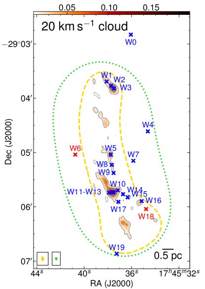
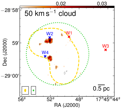
Figure 4: VLA H₂O masers in the six clouds. The background images and contours show the SMA 1.3 mm continuum emission, and the dashed and dotted loops show the mosaic field of the SMA and VLA, which are identical to those in Figure 3. H₂O masers are marked by crosses, among which red ones are those with AGB star counterparts.

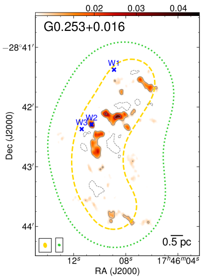
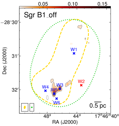
Figure 4: (Continued)

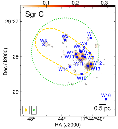
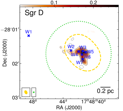
Figure 4: (Continued)

Table 5: Properties of H ii regions.

H ii region ID	R.A. & Decl.	$F_{\nu}$	$\log_{\text{10}}N_{\text{c}}$	Spectral type	ZAMS mass	References & Alternative identifiers
	(J2000)	(mJy)	(s-1)		($M_{\odot}$)
20 km s-1 H1	17:45:37.59, $-$29:05:43.60	1.5	46.00	B0.5	12	Lu et al. 2017
H2	17:45:38.00, $-$29:05:45.37	148.3	48.00	O9	20	Ho et al. 1985, Sgr A-G
50 km s-1 H1	17:45:52.23, $-$28:59:27.78	481.9	48.51	O7.5	26	Mills et al. 2011, Sgr A-A
H2	17:45:52.23, $-$28:59:37.97	129.1	47.94	O9	20	Mills et al. 2011, Sgr A-B
H3	17:45:52.65, $-$28:59:59.00	165.7	48.05	O8.5	21	Mills et al. 2011, Sgr A-C
H4	17:45:51.59, $-$29:00:22.40	111.0	47.88	O9	19	Mills et al. 2011, Sgr A-D
Sgr B1-off H1	17:46:47.10, $-$28:32:07.09	0.5	45.53	B1-B0.5	11	$\cdots$
Sgr C H1	17:44:41.20, $-$29:27:55.39	2.3	46.19	B0.5	13	$\cdots$
H2	17:44:40.92, $-$29:28:05.00	0.7	45.68	B1-B0.5	11	$\cdots$
H3	17:44:40.19, $-$29:28:15.20	5.0	46.53	B0.5	14	Forster & Caswell 2000, 359.44$-$0.10 A
H4	17:44:40.51, $-$29:28:16.99	14.9	47.00	B0	15	Forster & Caswell 2000
Sgr D H1	17:48:41.46, $-$28:01:40.90	1025.8	47.77	O9	19	Liszt 1992

3.4 VLA Radio Continuum Emission

Radio continuum emission at 23 GHz obtained by the VLA is displayed as green contours in Figure 3. There are several known H ii regions: one in the 20 km s^-1 cloud (Ho et al., 1985), four in the 50 km s^-1 cloud (Goss et al., 1985; Mills et al., 2011), and one in Sgr D (Liszt, 1992). Our observations confirmed radio continuum emission from them. We also detected several fainter compact sources that are associated with dust emission, which may be embedded UC H ii regions. Among them, the nature of the radio continuum in G0.253+0.016 has been discussed in Rodríguez & Zapata (2013) and Mills et al. (2015); one UC H ii region in Sgr C has been studied in Forster & Caswell (2000) and Kendrew et al. (2013); the UC H ii region in the 20 km s^-1 cloud has been reported in Lu et al. (2017). In addition, we found one compact radio continuum source in Sgr B1-off that is associated with a core, and several in Sgr C that have likely dust emission counterparts. Their nature will be discussed in Section 4.1.2. The detections are named with the letter ‘H’ plus a number by decreasing declinations in each cloud, and are marked in Figure 3. In general, their morphologies are not ellipse-like, so we did not fit 2D Gaussians to them, but measured their fluxes above the 3$\sigma$ level contour and listed the results in Table 5.

Filamentary radio continuum emission of $>$1 pc is seen in the 20 km s^-1 cloud and Sgr B1-off. Such structure in the CMZ has been suggested to have non-thermal origins (Ho et al., 1985; Lu et al., 2003; Zhao et al., 2016). As these are not related to recent star formation, we do not consider them further in this paper. Several compact radio continuum emission peaks without dust emission counterparts are also found (e.g., in Sgr C). They may be associated with more evolved H ii regions at late evolutionary phases, therefore are not considered either.

3.5 VLA H₂O Masers

In our previous work (Lu et al., 2015), we reported the detection of 18 H₂O masers in the 20 km s^-1 cloud. Here we searched for H₂O masers in all the six clouds in our sample. All point sources with peak intensities above the 8$\sigma$ level were identified, where 1$\sigma$ is $\sim$5 mJy beam^-1 in 0.2 km s^-1 velocity bin (see Table 2), but we excluded those found in dynamic-range limited channels, where the rms is significantly higher than the theoretical sensitivity, as these are likely sidelobes of strong sources. Multiple velocity components along the same line of sight were counted as a single maser. In addition, several strong masers were found outside the FWHM of the VLA primary beams. For example, in the 20 km s^-1 cloud, we found two masers close to or outside of the VLA primary beam boundaries in addition to the 18 masers reported in Lu et al. (2015). Such masers are also seen in the 50 km s^-1 cloud, Sgr C, and Sgr D. We took them into account if their peak intensities are above the 10$\sigma$ level. A total of 56 H₂O masers were identified in the six clouds.

We fit 2D Gaussians to the integrated intensity maps of the masers to determine their positions and integrated fluxes. The results are listed in Table 6, while the positions are marked in Figure 4 and the complete spectra shown in Appendix B. The masers are named by decreasing declinations in each cloud. Note that in the 20 km s^-1 cloud, we started with ‘W0’ that is outside of the VLA primary beams, in order to be consistent with the catalog in Lu et al. (2015), while in the other clouds we started with ‘W1’.

The coordinates and fluxes of the masers in the 20 km s^-1 cloud are slightly different from those reported in Lu et al. (2015), but are still within the pointing or flux calibration uncertainties (position differences $<$0.3″, flux differences $<$10%). This is likely because we applied the self-calibration solutions which slightly changed the phase and amplitude of the data.

While a good spatial correlation between H₂O masers and dust emission is generally found in Figure 4, it is interesting to note that several H₂O masers in G0.253+0.016 (e.g., W1 and W3) and Sgr B1-off (e.g., W1) do not seem to be associated with any dust emission. They may be unrelated to star formation and will be further discussed in Section 4.1.1.

4 Discussion

4.1 Signatures of Embedded Star Formation

We discuss signatures of star formation associated with the cores, and compare densities and virial states of the protostellar and starless core candidates.

Table 6: Properties of H₂O masers.

Maser ID	R.A. & Decl.	$v_{\text{peak}}$	$F_{\text{peak}}$	$F_{\text{integrated}}$	$L_{\text{H${}_{2}$O}}$	Cores/clumps	Other masers
	(J2000)	(km s-1)	(mJy per channel)	(mJy$\cdot$km s-1)	(10-7 $L_{\odot}$)
20 km s-1 W0	17:45:36.06, $-$29:02:49.73	$-$29.7	493	1090	16.6	$\cdots$
W1	17:45:38.10, $-$29:03:41.58	14.8	713	491	7.5	C1P2
W2	17:45:37.73, $-$29:03:46.18	27.8	240	946	14.4	C1P1
W3	17:45:37.49, $-$29:03:49.02	28.0	1568	4320	65.7	C1P1
W4	17:45:34.63, $-$29:04:36.62	2.4	686	852	12.9	$\cdots$
W5	17:45:37.76, $-$29:05:02.28	18.6	15377	7153	108.7	C3P1
W6	17:45:40.75, $-$29:05:02.29	12.7	317	418	6.4	AGB star
W7	17:45:35.85, $-$29:05:09.13	51.0	274	242	3.7	$\cdots$
W8	17:45:37.68, $-$29:05:13.68	46.2	38	49	0.7	C3P2
W9	17:45:37.52, $-$29:05:22.75	$-$40.0	50	100	1.5	C3P2
W10	17:45:37.16, $-$29:05:42.07	10.8	124	337	5.1	C4
W11	17:45:37.62, $-$29:05:44.24	4.4	919	3738	56.8	C4P1
W12	17:45:37.53, $-$29:05:44.11	9.3	192	411	6.2	C4P1
W13	17:45:37.92, $-$29:05:45.05	26.4	49	153	2.3	C4P1
W14	17:45:36.72, $-$29:05:46.23	$-$24.6	204	327	5.0	C4P5
W15	17:45:36.33, $-$29:05:49.82	13.1	1454	2762	42.0	C4P4
W16	17:45:35.15, $-$29:05:53.92	$-$4.4	64	94	1.4	C4P3
W17	17:45:37.10, $-$29:05:54.75	$-$3.8	222	360	5.5	C4P6
W18	17:45:34.78, $-$29:06:02.90	20.7	56	95	1.4	AGB star
W19	17:45:37.25, $-$29:06:52.03	$-$46.3	186	349	5.3	$\cdots$
50 km s-1 W1	17:45:49.41, $-$28:58:48.72	$-$3.9	844	1432	21.8	AGB star
W2	17:45:52.10, $-$28:58:50.06	37.6	94	263	4.0	C1P1
W3	17:45:44.31, $-$28:59:12.59	77.6	589	2790	42.4	AGB star
W4	17:45:52.73, $-$28:59:24.40	156.0	64	17	0.3	$\cdots$
G0.253+0.016 W1	17:46:08.90, $-$28:41:22.44	70.8	43	36	0.5	$\cdots$
W2	17:46:10.62, $-$28:42:17.44	39.0	262	541	8.2	C3P1
W3	17:46:11.38, $-$28:42:22.13	28.4	267	372	5.6	$\cdots$
Sgr B1-off W1	17:46:44.39, $-$28:30:55.28	111.4	50	73	1.1	$\cdots$
W2	17:46:43.41, $-$28:31:51.90	59.8	70	188	2.8	AGB star
W3	17:46:46.29, $-$28:31:58.28	27.9	57	21	0.3	C2P2
W4	17:46:48.23, $-$28:32:01.68	31.7	869	945	14.4	$\cdots$
W5	17:46:47.05, $-$28:32:06.97	30.5	360	364	5.5	C2P1	class ii CH3OH
W6	17:46:46.73, $-$28:32:15.69	$-$42.2	59	24	0.4	$\cdots$
Sgr C W1	17:44:40.21, $-$29:27:28.09	$-$52.8	302	469	7.1	$\cdots$
W2	17:44:43.56, $-$29:27:31.71	$-$47.7	551	587	8.9	C1P1
W3	17:44:46.37, $-$29:27:39.35	2.2	31	40	0.6	C2P1
W4	17:44:41.11, $-$29:27:44.26	3.9	48	301	4.6	$\cdots$
W5	17:44:41.59, $-$29:27:49.73	$-$53.8	44	43	0.7	C3
W6	17:44:41.50, $-$29:27:51.88	$-$55.3	94	96	1.5	C3
W7	17:44:42.11, $-$29:27:55.62	$-$53.0	5341	9037	137.4	C3P2
W8	17:44:41.29, $-$29:27:58.65	$-$56.0	798	2495	37.9	C3P1
W9	17:44:40.98, $-$29:28:00.78	$-$50.9	88	105	1.6	C3P1
W10	17:44:42.01, $-$29:28:00.84	$-$53.0	180	373	5.7	C3P2
W11	17:44:41.53, $-$29:28:06.22	$-$51.3	3764	2760	42.0	C3P3
W12	17:44:40.17, $-$29:28:12.68	$-$58.7	24754	42370	644.0	C4P2	class ii CH3OH
W13	17:44:40.60, $-$29:28:16.28	$-$57.8	7263	12700	193.0	C4P1	OH (1665 MHz), class ii CH3OH
W14	17:44:42.90, $-$29:28:17.04	$-$67.1	376	596	9.0	C5P1
W15	17:44:41.40, $-$29:28:29.67	$-$61.6	8179	8152	123.9	$\cdots$
W16	17:44:38.22, $-$29:29:12.61	$-$0.5	2075	8360	127.1	$\cdots$
Sgr D W1	17:48:48.55, $-$28.01.10.88	$-$13.3	7191	11450	14.8	$\cdots$	class ii CH3OH
W2	17:48:42.96, $-$28.01.37.12	$-$22.8	90	110	0.1	C1P5
W3	17:48:41.39, $-$28.01.38.25	$-$9.3	1885	5144	6.6	C1P1
W4	17:48:41.95, $-$28.01.38.69	$-$21.3	27	40	0.05	C1P4
W5	17:48:41.02, $-$28.01.39.97	$-$24.1	30	86	0.1	C1P2
W6	17:48:41.51, $-$28.01.44.00	3.1	5550	7302	9.4	C1P1
W7	17:48:41.42, $-$28.01.52.17	$-$24.9	301	576	0.7	C1P3

4.1.1 H₂O Masers

H₂O masers have been detected in both low-mass ($\leq$2 $M_{\odot}$) and high-mass ($\geq$8 $M_{\odot}$) star forming regions (Furuya et al., 2003; Szymczak et al., 2005; Urquhart et al., 2011) and are suggested to be associated with protostellar outflows (Elitzur et al., 1989; Codella et al., 2004). However, they may also be detectable toward the atmosphere of AGB stars. We compare our maser detections with the AGB star catalogs of Lindqvist et al. (1992), Sevenster et al. (1997), Sjouwerman et al. (1998, 2002), and Messineo et al. (2002), which are based on detections of OH/SiO masers, and with the catalog of Robitaille et al. (2008), which is based on infrared color criteria. Five of the H₂O masers have AGB star counterparts and are marked as red crosses in Figure 4: W6 and W18 in the 20 km s^-1 cloud, W1 and W3 in the 50 km s^-1 cloud, and W2 in Sgr B1-off. We thus excluded them in the following analysis. It is also possible that the AGB star catalogs are incomplete, therefore there may be more contamination from uncataloged AGB stars.

Another possibility is that the masers are created by pc-scale shocks, similar to the case of wide-spread class i CH₃OH masers found in the CMZ (Yusef-Zadeh et al., 2013). However, as we have argued in Lu et al. (2015), this is unlikely for most H₂O masers we detected, given their strong spatial correlation with the cores and their largely scattered velocities. For the eight H₂O masers not associated with detectable dust emission in the 50 km s^-1 cloud (W4), G0.253+0.016 (W1, W3), Sgr B1-off (W1, W4, W6), and Sgr C (W4, W15), however, this is a viable scenario. Alternatively, these masers may be associated with low-mass protostellar cores that are missed by our observations (e.g., below the 5$\sigma$ mass sensitivity of 22 $M_{\odot}$) or uncataloged AGB stars.

There are also six H₂O masers detected outside of the SMA mosaic fields and not associated with known AGB stars or other types of masers, including W0, W4, W7, and W19 in the 20 km s^-1 cloud, and W1 and W16 in Sgr C (but excluding W1 in Sgr D that is associated with a class ii CH₃OH maser, see Section 4.1.3), therefore their association with dust emission is unknown and their nature cannot be determined.

Thus, we conclude that most (37 out of 56, a percentage of 66%) of the detected H₂O masers are likely associated with star formation activities. It is unclear whether they trace low-mass or high-mass star formation. If we adopt the empirical correlation between the luminosities of H₂O masers and young stellar objects (e.g., Urquhart et al., 2011), then the more luminous H₂O masers ($\gtrsim$10^-6 $L_{\odot}$) would be associated with high-mass young stellar objects. As listed in Table 6, there are 19 such masers in our observations, and we note that some of them are associated with UC H ii regions or class ii CH₃OH masers, which signify high-mass star formation (see the next two sections). However, the scatter in the correlation of Urquhart et al. (2011) is large, and due to the time variability of H₂O masers, their luminosities can change by several orders of magnitude over several years (Felli et al., 2007). We cannot rule out the possibility that some of the fainter masers are associated with high-mass star formation, or that some of the luminous H₂O masers trace low-mass star formation.

4.1.2 H ii Regions

H ii regions are created by high-mass protostars of O or early-B types (Churchwell, 2002). As shown in Section 3.4, we confirm the existence of H ii regions in the 20 km s^-1 cloud, the 50 km s^-1 cloud, and Sgr D using the VLA radio continuum emission. In addition, several potential UC H ii regions of $<$0.1 pc scales are identified in the 20 km s^-1 cloud, Sgr B1-off, and Sgr C, and marked in Figure 3. We do not know their spectral indices, therefore are unable to verify whether the radio continuum emission represents a thermal free-free component. However, the close spatial correlations with compact dust emission suggest that they are more likely to be UC H ii regions embedded in cores. Note that in G0.253+0.016 we detect radio continuum emission towards the core C2P1, but this emission has been suggested to be unrelated to star formation (Mills et al., 2011, labeled as C3 in their Figure 2). C2P1 is gravitationally unbound according to our virial analysis in Section 3.2 and is unlikely to form stars. Therefore, this emission is not identified as an UC H ii region.

The ionizing photon fluxes of H ii regions $N_{\text{c}}$ are estimated from their radio continuum emission, assuming optically thin free-free emission and an electron temperature of 10⁴ K, following Mezger et al. (1974). Then assuming that each of the H ii regions is powered by a single star, we determine spectral types of the ionizing sources by comparing to the fluxes of ZAMS stars in Panagia (1973) and Davies et al. (2011), and estimate their stellar masses. The results are listed in Table 5.

4.1.3 Other Types of Masers from Literature

Early evolutionary phases of star formation in these clouds are also revealed by OH masers and CH₃OH masers. OH masers have also been detected toward AGB stars, as discussed in Section 4.1.1. Meanwhile, radiatively excited class ii CH₃OH masers have been suggested to uniquely trace high-mass star formation (Menten, 1991; Ellingsen, 2006; Breen et al., 2013).

We compare our results with the OH masers from catalogs in Karlsson et al. (2003) and Cotton & Yusef-Zadeh (2016). Among the four ground-state OH maser lines, the sole detection of the one at 1720 MHz, without accompanying main OH lines (at 1665/1667 MHz) or other maser species, usually traces supernova remnants (Wardle & Yusef-Zadeh, 2002). Similarly, the sole detection of the 1612 MHz OH maser is usually indicative of AGB stars, as discussed in Section 4.1.1. After excluding the supernova remnant or AGB star candidates, only one OH maser at 1665 MHz from Cotton & Yusef-Zadeh (2016) is found to be spatially coincident with the H₂O maser W13 and the core C4P1 in Sgr C.

The class ii CH₃OH maser catalog is taken from Caswell et al. (2010). Four masers are found, in Sgr B1-off towards W5/C2P1, in Sgr C toward W12/C4P2 and W13/C4P1, and in Sgr D towards W1. Their H₂O maser counterparts are bright ($\gtrsim$10^-6 $L_{\odot}$), consistent with being associated with high-mass star formation (Section 4.1.1).

Therefore, we conclude that our H₂O maser observations recover all previously detected star formation sites traced by OH and class ii CH₃OH masers. Nevertheless, the detection of class ii CH₃OH masers helps to confirm high-mass star formation. We listed all these detections in the last column of Table 6.

4.1.4 Densities and Virial States of Protostellar and Starless Cores

We classify the cores in a straightforward way as ‘protostellar’, which are associated with H₂O masers and/or (UC) H ii regions, and ‘starless’, where none of the star formation indicators is detected. Excluding Sgr D, we find 21 protostellar core candidates and 28 starless core candidates in the five CMZ clouds, as indicated in Table 3. With our classification, the starless core sample may be contaminated (e.g., some of the objects may already harbor protostars), while the protostellar core sample is precise (i.e., all the cores in this sample are likely forming stars, minus potential contamination by AGB stars) but is likely incomplete.

One property that may be able to modulate star formation in these cores is the density $n$(H₂). A wide variety of recent papers (Kruijssen et al., 2014; Rathborne et al., 2014; Krumholz & Kruijssen, 2015; Federrath et al., 2016; Krumholz et al., 2017; Ginsburg et al., 2018) have predicted or measured a density threshold for star formation in the CMZ of 10⁵–10⁷ cm^-3, which is much higher than the threshold in the Galactic disk clouds, $\sim$10⁴ cm^-3 (Lada et al., 2012). The other property significantly affecting star formation is the virial parameter $\alpha_{\text{vir}}$ (see Section 3.2), which determines the gravitational boundness of the cores. In Figure 5a, we plot these two properties of the protostellar and starless core candidates.

It is clear from Figure 5a that the protostellar core candidates tend to have higher densities and smaller virial parameters than the starless core candidates. We run a Kolmogorov-Smirnov (K-S) test to quantify how different the two samples are in terms of densities and virial parameters. Usually when the p-value is much smaller than 0.05, the difference between the two samples is significant, and when the $p$-value is much larger than 0.05, the difference is not significant and we cannot rule out the possibility that the two samples are drawn from the same distribution. The $p$-values from the K-S test of the densities or virial parameters of the two samples are $<$4$\times$10^-4, suggesting the difference between the two samples is statistically significant.

However, we do not find a clear density or virial parameter threshold between the protostellar and starless core candidates. The lowest density found in protostellar core candidates is 1.0$\times$10⁵ cm^-3, which is one order of magnitude lower than the highest density found in starless core candidates, 12.7$\times$10⁵ cm^-3. On the other hand, 7 out of the 21 protostellar core candidates have virial parameters $>$2, while small virial parameters of 1.1–1.3 are found in three starless core candidates. In Figure 5a, we show these criteria as shaded regions.

If we consider the densities and virial parameters jointly, then the cores having both virial parameters $<$6 (or a physically more meaningful threshold of $<$2) and densities above 4.5$\times$10⁵ cm^-3 are all protostellar candidates. Likewise, the core having both virial parameters $>$2 and densities below 4.5$\times$10⁵ cm^-3 are all starless candidates (except C4P5 in the 20 km s^-1 cloud, which is protostellar but spatially unresolved, so its density is a lower limit and its virial parameter is an upper limit). However, this does not suggest a clear criterion for separating the two samples, given the exceptions discussed below.

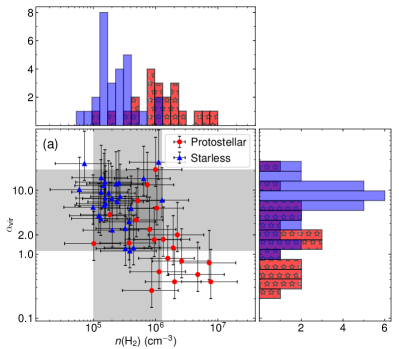
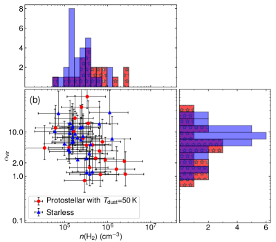
Figure 5: Densities and virial parameters of the protostellar and starless core candidates in the five clouds. Horizontal error bars show uncertainties in densities of 66%, while vertical error bars show uncertainties in virial parameters of 120% (factor 2.2). (a) The vertical shaded area spans densities of 1.0$\times$10⁵ cm^-3 to 12.7$\times$10⁵ cm^-3, representing the sufficient and the necessary density criteria for protostellar cores, respectively. Similarly, the horizontal shaded area spans between virial parameters of 20.9 and 1.12, representing the sufficient and the necessary virial parameter criteria for protostellar cores. (b) Same as the first panel but the densities and virial parameters of the protostellar core candidates are derived assuming a dust temperature of 50 K.

One protostellar core candidates, C2P1 in Sgr C, has a density of 1.0$\times$10⁵ cm^-3 that is 10 times lower than the median density of the protostellar core candidates and than most of the starless core candidates, even though its virial parameter is $<$2 suggesting that it is gravitationally bound and unstable to collapse. Its small density indicates that it is not as compact as the other protostellar cores, which can happen if it is at an earlier evolutionary phase than the others and collapse has just started, or if it only harbors lower mass protostars.

As stated above, there are seven protostellar core candidates with virial parameters $>$2. If outflows already exist in these cores, the line widths may be broadened therefore the virial parameters may be overestimated. Another possibility is that they further fragment into multiple substructures, each of which is gravitationally bound but as a whole they are not.

The starless core candidates, which may be contaminated with star forming cores, tend to have lower densities and larger virial parameters than the protostellar core candidates in Figure 5a. In particular, all the cores in G0.253+0.016 show large virial parameters and may be unbound. In fact, it is a question whether or not these substructures should be called ‘cores’, because if they are indeed unbound, they will be transient objects and likely disperse in a dynamical time scale.

One potential bias of the analysis here is that dust temperatures in the protostellar core candidates may be higher than the assumed 20 K because of internal heating, in which case the masses and the densities would be overestimated (see Section 3.3). Assuming a higher dust temperature of 50 K for the protostellar core candidates, the densities will be 3 times smaller while the virial parameters will be 3 times larger. As shown in Figure 5b, in this case the difference between the protostellar and starless core candidates is not significant, with $p$-values of $>$0.05 in the K-S test of densities or virial parameters between the two samples.

Another potential bias is that the low-/intermediate-mass star formation in the CMZ clouds is largely unknown, which may be taking place at lower densities. Our SMA dust continuum observations are not sensitive to low-mass protostellar cores below 22 $M_{\odot}$ (corresponding to a density of 0.7$\times$10⁵ cm^-3 assuming a typical radius of 0.1 pc). Although we detect several H₂O masers of lower luminosities (several times 10^-8 $L_{\odot}$) that are usually found toward low-mass young stellar objects (Furuya et al., 2003), they are insufficient to account for the expected low-mass star formation. Assuming a stellar initial mass function (IMF) from Kroupa (2001), about 100 low-mass ($\leq$2 $M_{\odot}$) stars will form in company with each high-mass ($\geq$8 $M_{\odot}$) star. Therefore, a large fraction of the low-mass star formation activity is not revealed by our H₂O maser observations. Future interferometer observations with high angular resolution and sensitivity that is able to resolve low-mass protostellar cores will help to address the issue of low-mass star formation in the CMZ.

Table 7: SFRs of the five clouds in our sample plus Sgr B2 from the literature.

Cloud	Mass	Bound Mass	Bound Mass Fraction	Masses of embedded high-mass protostars	$M_{\text{cluster}}$	SFR
	(104 $M_{\odot}$)	(102 $M_{\odot}$)	(%)	($M_{\odot}$)	($M_{\odot}$)	(10-3 $M_{\odot}$ yr-1)
20 km s-1	32.0	22.5	0.7	12(H1), 8(W1), 9(W2), 13(W3), 14(W5), 12(W15)	603$\pm$193	2.0$\pm$0.6
50 km s-1	6.1	1.1	0.2	$\cdots$	$<$91	$<$0.3
G0.253+0.016	8.8	0.7	0.08	8(W2)	91$\pm$82	0.3$\pm$0.3
Sgr B1-off	13.7	5.4	0.4	11(H1)	91$\pm$82	0.3$\pm$0.3
Sgr C	2.4	21.0	9	13(H1), 11(H2), 14(H3), 15(H4), 8(W2), 15(W7), 12(W11), 8(W14)	803$\pm$223	2.7$\pm$0.7
Sgr B2	140	450	3.2	271 high-mass protostars (Ginsburg et al., 2018)	(2.6$\pm$0.1)$\times$104	86$\pm$3

4.2 SFRs of the Clouds

We attempt to estimate SFRs of the CMZ clouds based on the H₂O masers and UC H ii regions, which characterize star formation in deeply embedded phases. In this analysis, we exclude the more evolved H ii regions that are not embedded in cores (e.g., H2 in the 20 km s^-1 cloud and H1–H4 in the 50 km s^-1 cloud). We expect the resulting SFRs are more closely related to the observed gas than the SFRs estimated in longer time scales based on H ii regions or infrared luminosities, although evolutionary cycling between gas and stars still causes the ratio between both to evolve with time (Kruijssen & Longmore, 2014).

4.2.1 Derivation of the SFRs

First, we define the characteristic time scale. The typical lifetime of the UC H ii region phase is $\sim$0.3 Myr (Davies et al., 2011). The lifetime of the evolutionary phase traced by the H₂O masers is estimated to be $\sim$0.3 Myr (Breen et al., 2010). In general, we adopt a time scale of 0.3 Myr for the overall star formation activities traced by H₂O masers and UC H ii regions.

Second, we estimate the stellar mass that will be formed based on the observed star formation tracers. We assume a canonical multiple-power-law IMF following Kroupa (2001, Equation (2)), with stellar masses between 0.01 $M_{\odot}$ and 150 $M_{\odot}$.

We estimate how massive clusters should be given the observed numbers of high-mass protostars. The numbers of high-mass protostars are estimated by counting UC H ii regions and luminous H₂O masers ($\gtrsim$10^-6 $L_{\odot}$) associated with cores. When both UC H ii regions and H₂O masers are detected, we count them as one. This approach alleviates the problem of Poisson noise associated with the detection of H₂O masers. However, it still suffers from several uncertainties. As discussed in Section 4.1.1, using luminous H₂O masers as indicators of high-mass star formation is highly uncertain, and the multiplicity of protostars is also an issue.

In Appendix D, we obtain a relation between cluster masses $M_{\text{cluster}}$ and numbers of high-mass protostars (see Figure 20b) by running Monte-Carlo simulations. The fractional uncertainty in $M_{\text{cluster}}$ decreases when more high-mass protostars are detected (e.g., 86% for one detection and 25% for 10 detections).

Stellar masses of the five clouds estimated using this relation are listed in Table 7. Then divided by the characteristic time scale of 3$\times$10⁵ yr, we obtain the SFRs of the clouds as listed in Table 7 and plotted as blue dots in Figure 6. Note that the uncertainties in the SFRs of G0.253+0.016 and Sgr B1-off are as large as the derived SFRs themselves, therefore the SFRs of these two clouds should be treated as having an upper limit of 0.6$\times$10^-3 $M_{\odot}$ yr^-1.

To validate our approach, we apply it to the whole CMZ, using the H₂O maser survey of Walsh et al. (2014). This survey is a follow up of the HOPS survey (Walsh et al., 2011) that covers Galactic longitudes between 290° and 30° and Galactic latitudes between $-$0$\fdg$5 and 0$\fdg$5, and achieves a point source sensitivity of $<$0.2 Jy per 0.42 km s^-1 channel for most of the data. We only consider H₂O masers with peak fluxes $\geq$0.6 Jy, corresponding to luminosities of $\gtrsim$10^-6 $L_{\odot}$ at the distance of 8.1 kpc, and only count masers within $|l|<1$°. We find 112 such masers from the catalog of Walsh et al. (2014), among which 49 are in Sgr B2. This number should be a lower limit given the issues in detection rate and multiplicity, although the sample may be contaminated by AGB stars. Assuming each of them is associated with a high-mass protostar, we use Equation D2, which agrees well with our simulations in Appendix D. The total stellar mass to be formed is estimated to be 1.1$\times$10⁴ $M_{\odot}$, then dividing by the time scale of 0.3 Myr, we obtain a SFR of 0.04 $M_{\odot}$ yr^-1. This is lower by a factor of 1.5–3 than those estimated from infrared luminosities or free-free emission over the same area (0.06–0.12 $M_{\odot}$ yr^-1; Longmore et al., 2013a; Barnes et al., 2017), which is reasonable given the limitations of our mass measurements.

4.2.2 Comparing with SFRs in Previous Studies

We compare the derived SFRs of the clouds with results in previous studies. Kauffmann et al. (2017a) has estimated SFRs of these clouds based on (both compact and UC) H ii regions and class ii CH₃OH masers, which characterize star formation in a time scale of 1.1 Myr. Their results are marked as crosses in Figure 6a, and typical uncertainty in their estimate of SFRs is a factor of 2. The most significant difference is that we find $>$10 times lower SFR for the 50 km s^-1 cloud ($<$0.3$\times$10^-3 $M_{\odot}$ yr^-1 vs. 3.2$\times$10^-3 $M_{\odot}$ yr^-1). Kauffmann et al. (2017a) took the four H ii regions in this cloud into account. Kauffmann et al. (2017b) noted the disconnection between the active star formation traced by the four H ii regions and a lack of massive clumps in this cloud. Our result suggests inactive star formation in the 50 km s^-1 cloud in the last 0.3 Myr (one weak H₂O maser, no signatures of high-mass star formation), which is consistent with the observed dearth of cores.

The SFR of Sgr C we derive is a factor of 3.4 higher than Kauffmann et al. (2017a): (2.7$\pm$0.7)$\times$10^-3 $M_{\odot}$ yr^-1 vs. 0.8$\times$10^-3 $M_{\odot}$ yr^-1. Given the large uncertainties in our estimate, this difference is not considered to be significant.

For the other three clouds, including the 20 km s^-1 cloud, G0.253+0.016, and Sgr B1-off, the SFRs in this work and in Kauffmann et al. (2017a) generally agree within a factor of 3, and are $\sim$10 times lower than expected by the linear correlation in Lada et al. (2010).

In addition, Barnes et al. (2017) estimated embedded stellar population of G0.253+0.016 and Sgr B1-off (named as Brick and clouds e & f, respectively, in their Tables 4 & 5) using infrared luminosities, and found $>$10 times higher stellar masses, which are upper limits, as the infrared luminosities have non-negligible contributions from other sources (e.g., external radiation, the diffuse infrared field at the Galactic center).

4.2.3 The SFR of Sgr B2

We estimate the SFR of Sgr B2 using data from the literature. The star formation at early evolutionary phases in Sgr B2 was recently studied by Ginsburg et al. (2018), who detected 271 compact continuum emission sources at 3 mm using ALMA, which are argued to be a mix of hyper-compact H ii regions and (high-mass) young stellar objects. Assuming that these 271 compact sources represent similar evolutionary phases as our H₂O maser and UC H ii sample, we estimate a total stellar mass of (2.6$\pm$0.1)$\times$10⁴ $M_{\odot}$ using Equation D2, and obtain a SFR of 0.086$\pm$0.003 $M_{\odot}$ yr^-1 in a time scale of 0.3 Myr.

Our result is 40% larger than the result of 0.062 $M_{\odot}$ yr^-1 reported in Ginsburg et al. (2018). The difference comes from both the stellar masses and the assumed time scales. Ginsburg et al. (2018) obtained a stellar mass of 3.3$\times$10⁴ $M_{\odot}$ when only considering sources not associated with H ii regions, which is 30% larger than our result, mostly because of different stellar masses attributed to each source. This indicates an additional uncertainty of 30% for the stellar masses in Sgr B2 from source classification. Ginsburg et al. (2018) also used a time scale of 0.74 Myr that is based on the dynamical model of Kruijssen et al. (2015), which is longer than our assumption of 0.3 Myr. Our result is also a factor of 2.4 larger than the result of 0.036 $M_{\odot}$ yr^-1 in Kauffmann et al. (2017a), which is based on the detection of 49 compact H ii regions in a time scale of 1.1 Myr.

Overall, we do not find significantly different SFRs for Sgr B2 from different approaches, and the discrepancy mostly comes from different assumed time scales. We summarize our estimate in Table 7.

4.2.4 Comparing with the Orbital Model of the CMZ

We compare our results with the orbital model of Kruijssen et al. (2015). This model suggests that all major clouds in the CMZ are subject to the gravitational potential around the Galactic Center and move in several gas streams (see the green curve in Figure 1). It also suggests that star formation in clouds could be triggered by tidal compression during a close passage to the bottom of the gravitational potential well near Sgr A*.

In the model of Kruijssen et al. (2015), G0.253+0.016, Sgr B1-off, and Sgr B2 are moving along one gas stream and have passed the pericenter to Sgr A*. Sgr C, the 20 km s^-1 cloud, and the 50 km s^-1 cloud are in the other gas stream, with Sgr C in the upstream, the 20 km s^-1 cloud approaching the pericenter, and the 50 km s^-1 cloud having passed the pericenter. As discussed previously and shown in Table 7, we find signatures of increasing SFRs from G0.253+0.016 to Sgr B1-off to Sgr B2, which agree with the proposed monotonic increase of the star formation activity along the direction of motion after passing by Sgr A* in this gas stream (Longmore et al., 2013b; Kruijssen et al., 2015). However, we do not find a similar trend for Sgr C, the 20 km s^-1 cloud, and the 50 km s^-1 cloud. The derived SFRs of Sgr C and the 20 km s^-1 cloud are similar given the uncertainties, and are higher than that of the 50 km s^-1 cloud. This may suggest that star formation in these clouds is not triggered by tidal compression when passing by the pericenter, but may be owing to self-gravity or impact of other sources (e.g., supernova remnants: Lu et al. 2003; Mills et al. 2011; H ii regions: Kendrew et al. 2013).

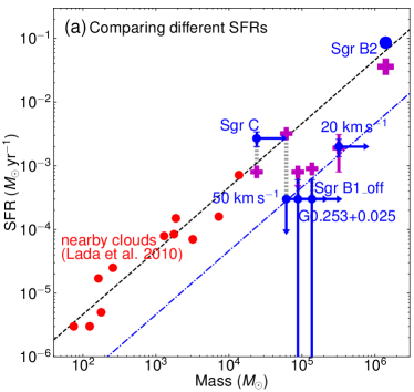
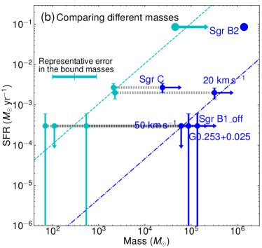
Figure 6: SFRs and masses of dense gas in the five CMZ clouds and in a sample of nearby clouds from Lada et al. (2010). Data of Sgr B2 compiled from the literature are also shown. (a) The blue dots mark the masses and SFRs of the five CMZ clouds in our observations plus Sgr B2. Errorbars, when presented, represent the errors listed in Table 7, and arrows suggest lower or upper limits. Each blue dot is connected to a magenta cross through a vertical line, which shows the SFR derived in Kauffmann et al. (2017a). The black dashed diagonal line marks the linear correlation in Lada et al. (2010), with red dots showing masses and SFRs of the nearby clouds based on which the correlation is derived. The blue dash-dotted diagonal line marks the expected relation when the SFR is 10 times lower. (b) The blue dots, errorbars, and the blue diagonal line are identical to those in (a). In addition, each blue dot is connected to a cyan dot through a horizontal line, which marks the gravitationally bound masses in Table 7. The horizontal cyan error bar represents the uncertainty in the gravitationally bound masses. The cyan dashed diagonal line is a linear fit to the cyan dots of the five CMZ clouds in our observations, with a slope of 10^-6 yr^-1. The big cyan dot for Sgr B2 denotes a gravitationally bound mass of 4.5$\times$10⁴ $M_{\odot}$, which is a lower limit.

4.3 Comparing with the Dense Gas Star Formation Relation

A quantitative comparison between star formation in these five CMZ clouds and that defined by the dense gas star formation relation has been done in Kauffmann et al. (2017a). Here we use the updated SFRs based on the H₂O masers and UC H ii regions to carry out this analysis. As discussed in Section 4.2, these SFRs characterize embedded star formation at very early evolutionary phases therefore are more closely related to the observed gas.

The cloud masses are taken from Kauffmann et al. (2017a), which are estimated using Herschel multi-wavelength data. The mean H₂ densities of these clouds are $\gtrsim$10⁴ cm^-3 (Kauffmann et al., 2017a), therefore the dense gas fraction as defined in Lada et al. (2010) is 100%—that is, all the gas in these clouds are supposed to be ‘dense’ and will collapse and form stars (but see Mills et al. 2018 for potential multiple density components in the 20 km s^-1 cloud, the 50 km s^-1 cloud, and G0.253+0.016, where $\sim$85% of the gas has a density of $<$10⁴ cm^-3). We then take the cloud masses to directly compare with the SFRs in the clouds.

The cloud masses and the SFRs of the five CMZ clouds (taken from Table 7) are plotted in Figure 6a. Given their masses, the SFR in Sgr C agrees with the linear correlation in Lada et al. (2010), while the SFRs in the other four clouds are $\sim$10 times lower than expected, around a linear relation with a slope of 5$\times$10^-9 yr^-1.

The linear relation between SFRs and gas masses can be written as (Lada et al., 2010)

$$\text{SFR}=\frac{\epsilon}{\tau_{\text{SF}}}\text{Mass},$$ (5)

in which $\epsilon$ is the SFE (the integrated efficiency of converting gas to stars) in the gas under consideration, and $\tau_{\text{SF}}$ is the time scale of star formation. Then over a time scale of 0.3 Myr, the SFE of the four clouds (the 20 km s^-1 cloud, the 50 km s^-1 cloud, G0.253+0.016, and Sgr B1-off) is 0.15%. This is significantly lower than those found in Galactic disk clouds, which are usually a few percent (Lada et al., 2010; Louvet et al., 2014).

In Section 4.1.4 we classify a sample of starless core candidates with large virial parameters, which may not form stars. Especially for G0.253+0.016, most of the cloud mass seems to be quiescent and irrelevant to high-mass star formation (Rathborne et al., 2014). It might make more sense to compare the masses in gravitationally bound cores, instead of those of the whole clouds, with the SFRs.

We attempt to estimate the gravitationally bound masses of the clouds by summing up masses of the protostellar core candidates and the prestellar core candidates that are gravitationally bound ($\alpha_{\text{vir}}$$\leq$2, see Table 3). In the following, we consider two systematic errors that significantly affect the estimate of the gravitationally bound masses and show that the uncertainty in the derived masses is a factor of 3.

First, the core identification in Section 3.1 is very likely incomplete, therefore the derived gravitationally bound masses are likely underestimated. To quantify how much mass may be missed, we estimate upper limits of the core masses in the 20 km s^-1 cloud and Sgr C by taking the total dust emission in the SMA maps into account. Most of the identified cores in these two clouds are protostellar and/or gravitationally bound, therefore we likely miss gravitationally bound gas in the core identification. We do not use the other three clouds for this estimate, because the cores in them are mostly unbound and the majority of the gas is clearly not involved in star formation. Then we derive masses using the total dust emission fluxes in the 20 km s^-1 cloud and Sgr C, which are upper limits to the gravitationally bound masses. These masses are 3 times higher than the derived bound masses.

Second, the derived masses are likely affected by the systematic error in the dust temperature owing to internal heating, since we take all the protostellar core candidates into account. As discussed in Section 3.3, the masses of cores with significant internal heating may be overestimated by a factor of 3.

We list the derived gravitationally bound masses in Table 7. In particular, Sgr C shows a high fraction of gravitationally bound mass (9%), while the other four clouds all have much smaller fractions ($<$1%). The derived gravitationally bound mass of Sgr C is similar to that of the 20 km s^-1 cloud. This has been noted in Kauffmann et al. (2017a) as a shallower mass-size slope in Sgr C than the other four clouds. It may explain the similar SFRs of Sgr C and the 20 km s^-1 cloud despite the fact that the cloud mass of Sgr C is only 7.5% of that of the 20 km s^-1 cloud.

Then we plot the gravitationally bound masses against the SFRs in Figure 6b. The five clouds can be fit by a linear function, with a slope of 10^-6 yr^-1, which indicates a gas consumption time of 1 Myr in these gravitationally bound cores. The linear relation is expected from a constant SFE. Following Equation 5, we obtain a SFE of 30% for the gas in the gravitationally bound/protostellar cores over a time scale of 0.3 Myr. Given the systematic errors in the derived gravitationally bound masses as discussed previously, the SFE may be as low as 10% and as high as 90%. This SFE is comparable to the value of 30%–40% for dense cores in nearby clouds (Alves et al., 2007; Könyves et al., 2015).

In addition, we include Sgr B2 in the analysis, while the data are compiled from the literature. The SFR at early evolutionary phases of 0.086$\pm$0.003 $M_{\odot}$ yr^-1 is based on the work of Ginsburg et al. (2018) (see Section 4.2.3). The cloud mass of Sgr B2 is taken to be 1.4$\times$10⁶ $M_{\odot}$ (Ginsburg et al., 2018, scaled to the distance of 8.1 kpc). The gravitationally bound mass is difficult to characterize and similar analysis to ours has not yet been published. As an approximate we use the total gas mass of the four protoclusters (Sgr B2 NE, N, M, and S), 4.5$\times$10⁴ $M_{\odot}$ (Schmiedeke et al., 2016, scaled to the distance of 8.1 kpc), which should be a lower limit given that the gas associated with the distributed protostellar population in Sgr B2 (Ginsburg et al., 2018) is not included. About 200 among the 271 compact sources found by Ginsburg et al. (2018) are not associated with any of the four protoclusters, therefore the total bound gas mass might be as much as four times larger than the mass in the four protoclusters if we assume the gas mass to be proportional to the number of compact sources. This results in a lower limit for the bound mass fraction of 3.3% for Sgr B2 that is potentially several times larger.

Comparing Sgr B2 with other clouds in Figure 6, we note that its SFR agrees with the star formation dense gas relation in Lada et al. (2010), similar to the case of Sgr C. Its bound gas mass fraction, with a lower limit of 3.3%, is also similar to Sgr C but 5–40 times larger than those of the other four clouds. When only considering the mass in the bound gas, Sgr B2 falls closely around the linear relation by fitting the five clouds in our sample, as shown in Figure 6b.

These results may suggest that star formation at the core scale in these CMZ clouds is not different from that in Galactic disk clouds in terms of the core to star-formation efficiency, but at the cloud scale, except for Sgr B2 and Sgr C, the star formation is $\sim$10 times less efficient because less than 1% of gas is confined in gravitationally bound regions. This small fraction of gravitationally bound gas in the clouds may be because of the strong turbulence in these clouds (Oka et al., 2001; Shetty et al., 2012; Kruijssen & Longmore, 2013) as indicated by the large line widths in the cores (Appendix C), or because the clouds have only recently condensed, as expected if the CMZ as a whole is undergoing episodic cycles of star formation activity (Kruijssen et al., 2014; Krumholz & Kruijssen, 2015; Krumholz et al., 2017).

5 CONCLUSIONS

We use the SMA 1.3 mm continuum and the VLA $K$-band continuum and H₂O maser observations to study star formation in five massive molecular clouds in the CMZ and one cloud that is likely outside of the CMZ. The main results are as follows.

• A total of 56 cores at the 0.2 pc scale are resolved by the SMA continuum emission in the six clouds. Their virial parameters are derived using line widths measured with the SMA N₂H⁺ or CH₃OH lines.

• In the five CMZ clouds, signatures of embedded star formation at very early evolutionary phases, as traced by H₂O masers and compact free-free emission from UC H ii regions, are found toward the cores, based on which we classify the cores as protostellar or starless. The protostellar core candidates tend to have higher densities and smaller virial parameters than the starless core candidates (Figure 5).

• Based on the detection of bright H₂O masers (with luminosities $\gtrsim$10^-6 $L_{\odot}$) and UC H ii regions, SFRs within a time scale of 0.3 Myr of the five CMZ clouds are estimated. We also include Sgr B2 in the analysis after compiling data from previous studies. The observed increasing SFRs from G0.253+0.016 to Sgr B1-off to Sgr B2 are expected by the CMZ orbital model of Kruijssen et al. (2015), but the SFRs of the other three clouds do not show a monotonic change that is predicted by this model.

• Excluding Sgr B2 and Sgr C, SFRs of the other four CMZ clouds are $\sim$10 times lower than expected from the dense gas star formation relation extrapolated from nearby clouds in Lada et al. (2010) (Figure 6a). If the masses in protostellar and/or gravitationally bound cores are used instead, these clouds can be better fit with a linear function, with a SFE of 30% over a time scale of 0.3 Myr (Figure 6b). Among the six CMZ clouds (five in our sample plus Sgr B2 from the literature), Sgr B2 and Sgr C stand out with larger fractions of mass in gravitationally bound regions and higher SFRs per unit cloud mass.

• We confirm that star formation in four of the CMZ clouds is inactive with respect to the prediction of the dense gas star formation relation, even after taking star formation at very early evolutionary phases into account. This is likely related to their low gravitationally bound gas fractions of $<$1%, which may be because of high turbulent energy densities in the CMZ and/or because they are dynamically young and have not had the time to populate their high-density component.

Appendix A Identification of substructures using Dendrogram

We identified compact structures (‘leaves’) in the SMA 1.3 mm continuum emission maps using the dendrogram algorithm (Rosolowsky et al., 2008) implemented with astrodendro. We adopted a minimum intensity of 4$\sigma$ where the $\sigma$ values can be found in Table 2, below which the emission will not be considered, and a minimum significance of 1$\sigma$, which characterizes the significance a local maxima has to reach to be considered as an independent structure. With this setup, the identified structures will have peak intensities above the 5$\sigma$ level. We additionally specified that the number of pixels above the 5$\sigma$ level in one structure must be larger than the pixel number within the FWHM of one synthesized beam. The results are presented in Figure 7, where the identified structures are marked by blue contours.

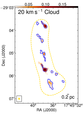
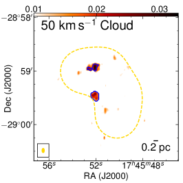
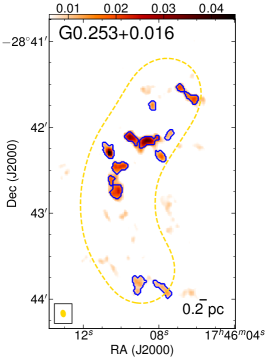
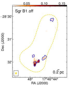
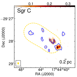
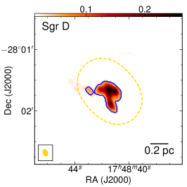
Figure 7: Result of the dendrogram analysis. Background images and dashed loops show the SMA 1.3 mm continuum and the SMA mosaic field, which are identical to those in Figure 3. Blue contours mark leaves identified using astrodendro.

This procedure occasionally misses obvious structures. For example, in the 20 km s^-1 cloud several emission peaks are spatially coincident with H₂O masers therefore should be protostellar core candidates (see Figure 4), but are not identified because their areas are slightly smaller than the beam size. Another example is that in Sgr C two adjacent bright structures in the southwestern end are identified as one because of their small projected spatial separation, but they should be two independent cores given that they are each associated with a UC H ii region and a H₂O maser (see Figures 3 & 4). Therefore, in Section 3.1 we used the outcome of astrodendro as a reference but manually added or removed structures in consideration of the above situations.

Appendix B H₂O maser spectra

We present the spectra of all the detected H₂O masers in the six clouds in Figures 8–13. The x-axis is $V_{\text{lsr}}$ in unit of km s^-1, while the y-axis is flux density in unit of mJy. Positions of the masers are marked in the maps in Figure 4. The labels of H₂O masers with OH/IR star counterparts are marked by red.

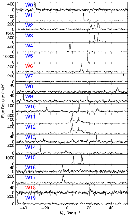
Figure 8: H₂O maser spectra in the 20 km s^-1 cloud detected by the VLA.

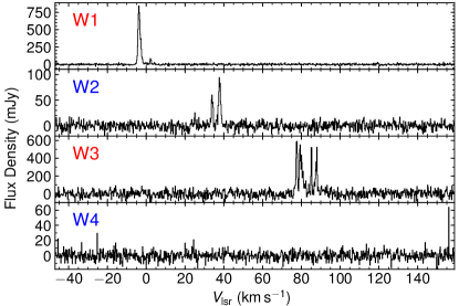
Figure 9: H₂O maser spectra in the 50 km s^-1 cloud detected by the VLA.

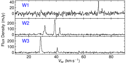
Figure 10: H₂O maser spectra in G0.253+0.016 detected by the VLA.

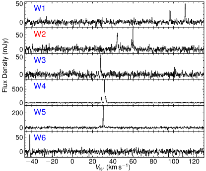
Figure 11: H₂O maser spectra in Sgr B1-off detected by the VLA.

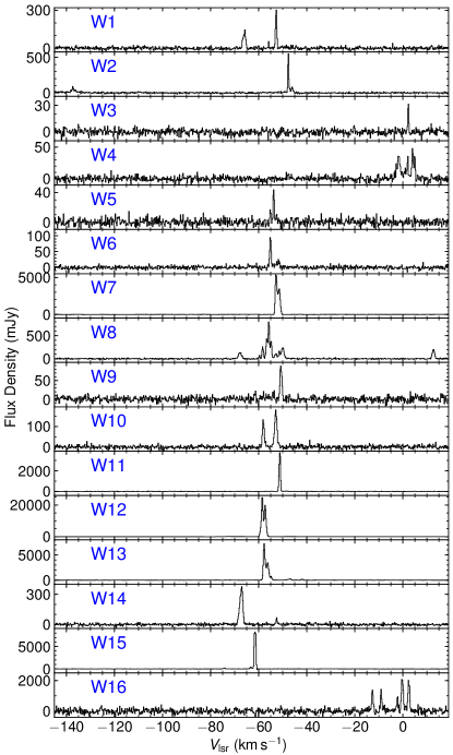
Figure 12: H₂O maser spectra in Sgr C detected by the VLA.

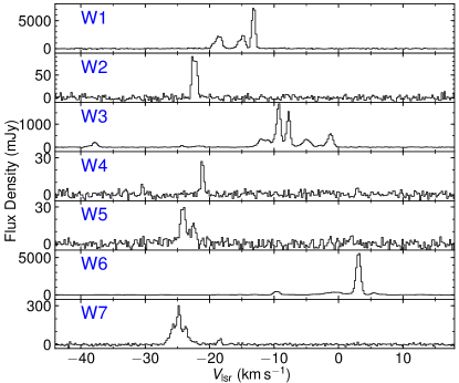
Figure 13: H₂O maser spectra in Sgr D detected by the VLA.

Appendix C Line widths in cores

We extract the mean spectra of N₂H⁺ 3–2 (Kauffmann et al., 2017a), or if it is not detected, those of CH₃OH 4₂₂–3₁₂ in our SMA data, toward the identified cores. Then for each spectrum, a single Gaussian is fit to obtain the line width. The results are shown in Figures 14–19.

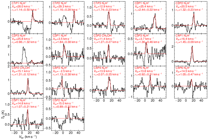
Figure 14: The SMA N₂H⁺ or CH₃OH spectra and best-fit models of cores in the 20 km s^-1 cloud. The best-fit centroid velocities ($V_{\text{lsr}}$) and line widths ($\sigma_{v}$, deconvolved from channel width) are noted in each panel.

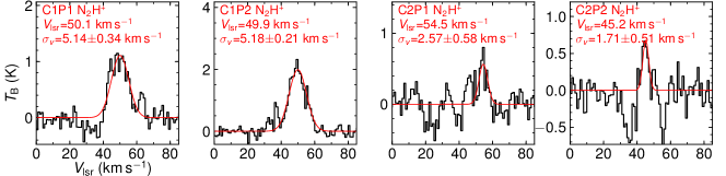
Figure 15: The SMA N₂H⁺ spectra and best-fit models of cores in the 50 km s^-1 cloud. The best-fit line widths (deconvolved from channel width) are noted in each panel.

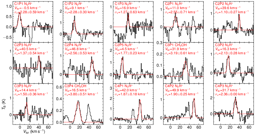
Figure 16: The SMA N₂H⁺ or CH₃OH spectra and best-fit models of cores in G0.253+0.016. The best-fit line widths (deconvolved from channel width) are noted in each panel.

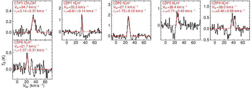
Figure 17: The SMA N₂H⁺ or CH₃OH spectra and best-fit models of cores in Sgr B1-off. The best-fit line widths (deconvolved from channel width) are noted in each panel.

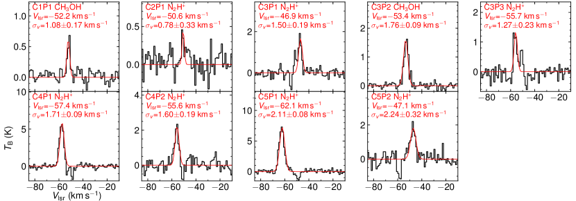
Figure 18: The SMA N₂H⁺ or CH₃OH spectra and best-fit models of cores in Sgr C. The best-fit line widths (deconvolved from channel width) are noted in each panel.

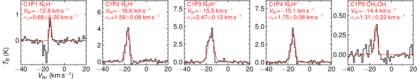
Figure 19: The SMA N₂H⁺ or CH₃OH spectra and best-fit models of cores in Sgr D. The best-fit line widths (deconvolved from channel width) are noted in each panel.

Appendix D Estimate of Cluster Masses through Monte-Carlo Simulations

In order to quantify the uncertainties in cluster masses stemming from the random sampling of stellar masses following the IMF as a probability distribution function, we run Monte-Carlo simulations to generate cluster masses, and find the relation between them and the number of high-mass ($\geq$8 $M_{\odot}$) stars in the cluster. The scripts to run these simulations are available at https://github.com/xinglunju/CMZclouds/tree/master/Mcluster.

Following the Bayes theorem, the posterior probability of cluster masses $M_{\text{cluster}}$ given that there are $N$ high-mass stars in the cluster is

$$\text{prob}(M_{\text{cluster}}|N)=\frac{\text{prob}(M_{\text{cluster}})\text{prob}(N|M_{\text{cluster}})}{\text{prob}(N)},$$ (D1)

in which $\text{prob}(M_{\text{cluster}})$ is the prior probability of $M_{\text{cluster}}$, $\text{prob}(N|M_{\text{cluster}})$ is the likelihood of having $N$ high-mass stars given a cluster mass of $M_{\text{cluster}}$, and $\text{prob}(N)$ is the evidence and usually treated as a normalizing factor.

We adopt a flat log-prior probability $\text{prob}(M_{\text{cluster}})$ in a range of $[10,2000]$ $M_{\odot}$, outside of which $\text{prob}(M_{\text{cluster}})$ is set to 0. To obtain the likelihood $\text{prob}(N|M_{\text{cluster}})$, we run Monte-Carlo simulations to generate stellar masses following the IMF (Equations 1 & 2 of Kroupa, 2001, with stellar masses between 0.01 $M_{\odot}$ and 150 $M_{\odot}$) as a probability distribution function until the total mass reaches $M_{\text{cluster}}$, and count the number of high-mass stars produced in this process. For each $M_{\text{cluster}}$, we run the simulation 10,000 times, and divide the number of the runs producing $N$ high-mass stars by 10,000 to get the likelihood $\text{prob}(N|M_{\text{cluster}})$. Finally, the posterior probability $\text{prob}(M_{\text{cluster}}|N)$ is proportional to $\text{prob}(N|M_{\text{cluster}})$, and is shown in Figure 20a.

The resulting posterior probability functions $\text{prob}(M_{\text{cluster}}|N)$ are skewed to the right side compared to a lognormal distribution. To better estimate peak locations, we fit Weibull distribution functions (Weibull, 1951) to $\text{prob}(M_{\text{cluster}}|N)$, shown in Figure 20a. We use the modes (peak locations) of the Weibull functions (therefore the most likely) as the final estimate of cluster masses, and the rms of the simulated data to approximate the uncertainties in the estimated masses.

In Figure 20b, we plot the cluster masses estimated above given $N$ high-mass stars in the cluster. The result agrees well with the analytical form directly derived from the IMF,

$$M_{\text{cluster}}=95.8\times N~{}\mbox{$M_{\odot}$},$$ (D2)

which is plotted as a dashed curve in Figure 20b. The simulations are able to give an estimate of uncertainties stemming from the random sampling of stellar masses following the IMF as a probability distribution function. In Section 4.2, we rely on the data points in Figure 20b to estimate cluster masses.

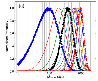
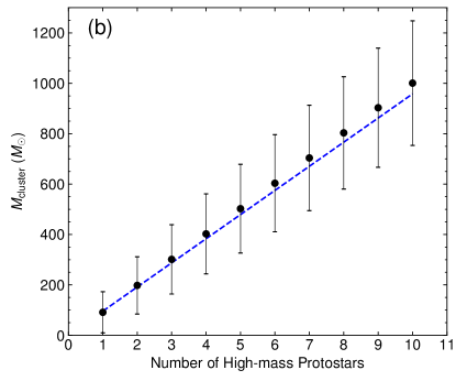
Figure 20: (a) Normalized probabilities of cluster masses given 1 to 10 high-mass stars produced in the cluster. Data points are results from simulations and solid curves are best-fit Weibull functions. For clarify of presentation, only data points of simulations with $N=1,4,7,10$ are plotted. (b) Expected cluster masses given the detection of a certain number of high-mass protostars. Vertical errorbars show the uncertainties in cluster masses.

References

- Alves et al. (2007) Alves, J., Lombardi, M., & Lada, C. J. 2007, A&A, 462, L17, doi: 10.1051/0004-6361:20066389
- An et al. (2011) An, D., Ramírez, S. V., Sellgren, K., et al. 2011, ApJ, 736, 133, doi: 10.1088/0004-637X/736/2/133
- Ao et al. (2013) Ao, Y., Henkel, C., Menten, K. M., et al. 2013, A&A, 550, A135, doi: 10.1051/0004-6361/201220096
- Astropy Collaboration et al. (2013) Astropy Collaboration, Robitaille, T. P., Tollerud, E. J., et al. 2013, A&A, 558, A33, doi: 10.1051/0004-6361/201322068
- Barnes et al. (2017) Barnes, A. T., Longmore, S. N., Battersby, C., et al. 2017, MNRAS, 469, 2263, doi: 10.1093/mnras/stx941
- Battersby et al. (2011) Battersby, C., Bally, J., Ginsburg, A., et al. 2011, A&A, 535, A128, doi: 10.1051/0004-6361/201116559
- Bertoldi & McKee (1992) Bertoldi, F., & McKee, C. F. 1992, ApJ, 395, 140, doi: 10.1086/171638
- Beuther et al. (2002) Beuther, H., Schilke, P., Menten, K. M., et al. 2002, ApJ, 566, 945, doi: 10.1086/338334
- Breen et al. (2010) Breen, S. L., Ellingsen, S. P., Caswell, J. L., & Lewis, B. E. 2010, MNRAS, 401, 2219, doi: 10.1111/j.1365-2966.2009.15831.x
- Breen et al. (2013) Breen, S. L., Ellingsen, S. P., Contreras, Y., et al. 2013, MNRAS, 435, 524, doi: 10.1093/mnras/stt1315
- Caselli et al. (2002) Caselli, P., Walmsley, C. M., Zucconi, A., et al. 2002, ApJ, 565, 331, doi: 10.1086/324301
- Caswell et al. (2010) Caswell, J. L., Fuller, G. A., Green, J. A., et al. 2010, MNRAS, 404, 1029, doi: 10.1111/j.1365-2966.2010.16339.x
- Churchwell (2002) Churchwell, E. 2002, ARA&A, 40, 27, doi: 10.1146/annurev.astro.40.060401.093845
- Codella et al. (2004) Codella, C., Lorenzani, A., Gallego, A. T., Cesaroni, R., & Moscadelli, L. 2004, A&A, 417, 615, doi: 10.1051/0004-6361:20035608
- Cornwell (2008) Cornwell, T. J. 2008, IEEE Journal of Selected Topics in Signal Processing, 2, 793, doi: 10.1109/JSTSP.2008.2006388
- Cotton & Yusef-Zadeh (2016) Cotton, W. D., & Yusef-Zadeh, F. 2016, ApJS, 227, 10, doi: 10.3847/0067-0049/227/1/10
- Davies et al. (2011) Davies, B., Hoare, M. G., Lumsden, S. L., et al. 2011, MNRAS, 416, 972, doi: 10.1111/j.1365-2966.2011.19095.x
- De Pree et al. (2015) De Pree, C. G., Peters, T., Mac Low, M. M., et al. 2015, ApJ, 815, 123, doi: 10.1088/0004-637X/815/2/123
- Draine (2011) Draine, B. T. 2011, Physics of the Interstellar and Intergalactic Medium (Princeton, NJ: Princeton University Press)
- Elitzur et al. (1989) Elitzur, M., Hollenbach, D. J., & McKee, C. F. 1989, ApJ, 346, 983, doi: 10.1086/168080
- Ellingsen (2006) Ellingsen, S. P. 2006, ApJ, 638, 241, doi: 10.1086/498673
- Federrath et al. (2016) Federrath, C., Rathborne, J. M., Longmore, S. N., et al. 2016, ApJ, 832, 143, doi: 10.3847/0004-637X/832/2/143
- Felli et al. (2007) Felli, M., Brand, J., Cesaroni, R., et al. 2007, A&A, 476, 373, doi: 10.1051/0004-6361:20077804
- Ferrière et al. (2007) Ferrière, K., Gillard, W., & Jean, P. 2007, A&A, 467, 611, doi: 10.1051/0004-6361:20066992
- Forster & Caswell (2000) Forster, J. R., & Caswell, J. L. 2000, ApJ, 530, 371, doi: 10.1086/308347
- Furuya et al. (2003) Furuya, R. S., Kitamura, Y., Wootten, A., Claussen, M. J., & Kawabe, R. 2003, ApJS, 144, 71, doi: 10.1086/342749
- Gao & Solomon (2004) Gao, Y., & Solomon, P. M. 2004, ApJ, 606, 271, doi: 10.1086/382999
- Giannetti et al. (2017) Giannetti, A., Leurini, S., König, C., et al. 2017, A&A, 606, L12, doi: 10.1051/0004-6361/201731728
- Ginsburg et al. (2016) Ginsburg, A., Henkel, C., Ao, Y., et al. 2016, A&A, 586, A50, doi: 10.1051/0004-6361/201526100
- Ginsburg et al. (2018) Ginsburg, A., Bally, J., Barnes, A., et al. 2018, ApJ, 853, 171, doi: 10.3847/1538-4357/aaa6d4
- Goss et al. (1985) Goss, W. M., Schwarz, U. J., van Gorkom, J. H., & Ekers, R. D. 1985, MNRAS, 215, 69P, doi: 10.1093/mnras/215.1.69P
- Gravity Collaboration et al. (2018) Gravity Collaboration, Abuter, R., Amorim, A., et al. 2018, A&A, 615, L15, doi: 10.1051/0004-6361/201833718
- Ho et al. (1985) Ho, P. T. P., Jackson, J. M., Barrett, A. H., & Armstrong, J. T. 1985, ApJ, 288, 575, doi: 10.1086/162823
- Ho et al. (2004) Ho, P. T. P., Moran, J. M., & Lo, K. Y. 2004, ApJ, 616, L1, doi: 10.1086/423245
- Immer et al. (2012) Immer, K., Schuller, F., Omont, A., & Menten, K. M. 2012, A&A, 537, A121, doi: 10.1051/0004-6361/201117857
- Johnston et al. (2014) Johnston, K. G., Beuther, H., Linz, H., et al. 2014, A&A, 568, A56, doi: 10.1051/0004-6361/201423943
- Karlsson et al. (2003) Karlsson, R., Sjouwerman, L. O., Sandqvist, A., & Whiteoak, J. B. 2003, A&A, 403, 1011, doi: 10.1051/0004-6361:20030309
- Kauffmann et al. (2008) Kauffmann, J., Bertoldi, F., Bourke, T. L., Evans, II, N. J., & Lee, C. W. 2008, A&A, 487, 993, doi: 10.1051/0004-6361:200809481
- Kauffmann et al. (2013) Kauffmann, J., Pillai, T., & Zhang, Q. 2013, ApJ, 765, L35, doi: 10.1088/2041-8205/765/2/L35
- Kauffmann et al. (2017a) Kauffmann, J., Pillai, T., Zhang, Q., et al. 2017a, A&A, 603, A89, doi: 10.1051/0004-6361/201628088
- Kauffmann et al. (2017b) —. 2017b, A&A, 603, A90, doi: 10.1051/0004-6361/201628089
- Kendrew et al. (2013) Kendrew, S., Ginsburg, A., Johnston, K., et al. 2013, ApJ, 775, L50, doi: 10.1088/2041-8205/775/2/L50
- Kennicutt (1998) Kennicutt, Jr., R. C. 1998, ApJ, 498, 541, doi: 10.1086/305588
- Könyves et al. (2015) Könyves, V., André, P., Men’shchikov, A., et al. 2015, A&A, 584, A91, doi: 10.1051/0004-6361/201525861
- Krieger et al. (2017) Krieger, N., Ott, J., Beuther, H., et al. 2017, ApJ, 850, 77, doi: 10.3847/1538-4357/aa951c
- Kroupa (2001) Kroupa, P. 2001, MNRAS, 322, 231, doi: 10.1046/j.1365-8711.2001.04022.x
- Kruijssen et al. (2015) Kruijssen, J. M. D., Dale, J. E., & Longmore, S. N. 2015, MNRAS, 447, 1059, doi: 10.1093/mnras/stu2526
- Kruijssen & Longmore (2013) Kruijssen, J. M. D., & Longmore, S. N. 2013, MNRAS, 435, 2598, doi: 10.1093/mnras/stt1634
- Kruijssen & Longmore (2014) —. 2014, MNRAS, 439, 3239, doi: 10.1093/mnras/stu098
- Kruijssen et al. (2014) Kruijssen, J. M. D., Longmore, S. N., Elmegreen, B. G., et al. 2014, MNRAS, 440, 3370, doi: 10.1093/mnras/stu494
- Krumholz & Kruijssen (2015) Krumholz, M. R., & Kruijssen, J. M. D. 2015, MNRAS, 453, 739, doi: 10.1093/mnras/stv1670
- Krumholz et al. (2017) Krumholz, M. R., Kruijssen, J. M. D., & Crocker, R. M. 2017, MNRAS, 466, 1213, doi: 10.1093/mnras/stw3195
- Lada et al. (2012) Lada, C. J., Forbrich, J., Lombardi, M., & Alves, J. F. 2012, ApJ, 745, 190, doi: 10.1088/0004-637X/745/2/190
- Lada et al. (2010) Lada, C. J., Lombardi, M., & Alves, J. F. 2010, ApJ, 724, 687, doi: 10.1088/0004-637X/724/1/687
- Lindqvist et al. (1992) Lindqvist, M., Winnberg, A., Habing, H. J., & Matthews, H. E. 1992, A&AS, 92, 43
- Liszt (1992) Liszt, H. S. 1992, ApJS, 82, 495, doi: 10.1086/191727
- Longmore et al. (2011) Longmore, S. N., Pillai, T., Keto, E., Zhang, Q., & Qiu, K. 2011, ApJ, 726, 97, doi: 10.1088/0004-637X/726/2/97
- Longmore et al. (2013a) Longmore, S. N., Bally, J., Testi, L., et al. 2013a, MNRAS, 429, 987, doi: 10.1093/mnras/sts376
- Longmore et al. (2013b) Longmore, S. N., Kruijssen, J. M. D., Bally, J., et al. 2013b, MNRAS, 433, L15, doi: 10.1093/mnrasl/slt048
- Louvet et al. (2014) Louvet, F., Motte, F., Hennebelle, P., et al. 2014, A&A, 570, A15, doi: 10.1051/0004-6361/201423603
- Lu et al. (2003) Lu, F. J., Wang, Q. D., & Lang, C. C. 2003, AJ, 126, 319, doi: 10.1086/375754
- Lu et al. (2015) Lu, X., Zhang, Q., Kauffmann, J., et al. 2015, ApJ, 814, L18, doi: 10.1088/2041-8205/814/2/L18
- Lu et al. (2017) —. 2017, ApJ, 839, 1, doi: 10.3847/1538-4357/aa67f7
- McMullin et al. (2007) McMullin, J. P., Waters, B., Schiebel, D., Young, W., & Golap, K. 2007, in ASP Conf. Ser., Vol. 376, Astronomical Data Analysis Software and Systems XVI, ed. R. A. Shaw, F. Hill, & D. J. Bell (San Francisco, CA: ASP), 127
- Menten (1991) Menten, K. 1991, in ASP Conf. Ser., Vol. 16, Atoms, Ions and Molecules: New Results in Spectral Line Astrophysics, ed. A. D. Haschick & P. T. P. Ho (San Francisco: ASP), 119
- Messineo et al. (2002) Messineo, M., Habing, H. J., Sjouwerman, L. O., Omont, A., & Menten, K. M. 2002, A&A, 393, 115, doi: 10.1051/0004-6361:20021017
- Mezger et al. (1974) Mezger, P. G., Smith, L. F., & Churchwell, E. 1974, A&A, 32, 269
- Mills et al. (2011) Mills, E., Morris, M. R., Lang, C. C., et al. 2011, ApJ, 735, 84, doi: 10.1088/0004-637X/735/2/84
- Mills et al. (2015) Mills, E. A. C., Butterfield, N., Ludovici, D. A., et al. 2015, ApJ, 805, 72, doi: 10.1088/0004-637X/805/1/72
- Mills et al. (2018) Mills, E. A. C., Ginsburg, A., Immer, K., et al. 2018, ApJ, 868, 7, doi: 10.3847/1538-4357/aae581
- Molinari et al. (2011) Molinari, S., Bally, J., Noriega-Crespo, A., et al. 2011, ApJ, 735, L33, doi: 10.1088/2041-8205/735/2/L33
- Morris & Serabyn (1996) Morris, M., & Serabyn, E. 1996, ARA&A, 34, 645, doi: 10.1146/annurev.astro.34.1.645
- Motte et al. (2003) Motte, F., Schilke, P., & Lis, D. C. 2003, ApJ, 582, 277, doi: 10.1086/344538
- Oka et al. (2001) Oka, T., Hasegawa, T., Sato, F., et al. 2001, ApJ, 562, 348, doi: 10.1086/322976
- Ossenkopf & Henning (1994) Ossenkopf, V., & Henning, T. 1994, A&A, 291, 943
- Panagia (1973) Panagia, N. 1973, AJ, 78, 929, doi: 10.1086/111498
- Pillai et al. (2015) Pillai, T., Kauffmann, J., Tan, J. C., et al. 2015, ApJ, 799, 74, doi: 10.1088/0004-637X/799/1/74
- Rathborne et al. (2014) Rathborne, J. M., Longmore, S. N., Jackson, J. M., et al. 2014, ApJ, 795, L25, doi: 10.1088/2041-8205/795/2/L25
- Robitaille & Bressert (2012) Robitaille, T., & Bressert, E. 2012, APLpy: Astronomical Plotting Library in Python, Astrophysics Source Code Library. http://ascl.net/1208.017
- Robitaille et al. (2008) Robitaille, T. P., Meade, M. R., Babler, B. L., et al. 2008, AJ, 136, 2413, doi: 10.1088/0004-6256/136/6/2413
- Rodríguez & Zapata (2013) Rodríguez, L. F., & Zapata, L. A. 2013, ApJ, 767, L13, doi: 10.1088/2041-8205/767/1/L13
- Rosolowsky et al. (2008) Rosolowsky, E. W., Pineda, J. E., Kauffmann, J., & Goodman, A. A. 2008, ApJ, 679, 1338, doi: 10.1086/587685
- Sakai et al. (2017) Sakai, D., Oyama, T., Nagayama, T., Honma, M., & Kobayashi, H. 2017, PASJ, 69, 64, doi: 10.1093/pasj/psx039
- Sanhueza et al. (2017) Sanhueza, P., Jackson, J. M., Zhang, Q., et al. 2017, ApJ, 841, 97, doi: 10.3847/1538-4357/aa6ff8
- Sault et al. (1995) Sault, R. J., Teuben, P. J., & Wright, M. C. H. 1995, in ASP Conf. Ser., Vol. 77, Astronomical Data Analysis Software and Systems IV, ed. R. A. Shaw, H. E. Payne, & J. J. E. Hayes (San Francisco, CA: ASP), 433
- Sawada et al. (2009) Sawada, M., Tsujimoto, M., Koyama, K., et al. 2009, PASJ, 61, S209, doi: 10.1093/pasj/61.sp1.S209
- Schmidt (1959) Schmidt, M. 1959, ApJ, 129, 243, doi: 10.1086/146614
- Schmiedeke et al. (2016) Schmiedeke, A., Schilke, P., Möller, T., et al. 2016, A&A, 588, A143, doi: 10.1051/0004-6361/201527311
- Sevenster et al. (1997) Sevenster, M. N., Chapman, J. M., Habing, H. J., Killeen, N. E. B., & Lindqvist, M. 1997, A&AS, 122, 79, doi: 10.1051/aas:1997294
- Shetty et al. (2012) Shetty, R., Beaumont, C. N., Burton, M. G., Kelly, B. C., & Klessen, R. S. 2012, MNRAS, 425, 720, doi: 10.1111/j.1365-2966.2012.21588.x
- Shirley (2015) Shirley, Y. L. 2015, PASP, 127, 299, doi: 10.1086/680342
- Sjouwerman et al. (2002) Sjouwerman, L. O., Lindqvist, M., van Langevelde, H. J., & Diamond, P. J. 2002, A&A, 391, 967, doi: 10.1051/0004-6361:20020983
- Sjouwerman et al. (1998) Sjouwerman, L. O., van Langevelde, H. J., Winnberg, A., & Habing, H. J. 1998, A&AS, 128, 35, doi: 10.1051/aas:1998127
- Szymczak et al. (2005) Szymczak, M., Pillai, T., & Menten, K. M. 2005, A&A, 434, 613, doi: 10.1051/0004-6361:20042437
- Urquhart et al. (2011) Urquhart, J. S., Morgan, L. K., Figura, C. C., et al. 2011, MNRAS, 418, 1689, doi: 10.1111/j.1365-2966.2011.19594.x
- Walker et al. (2018) Walker, D. L., Longmore, S. N., Zhang, Q., et al. 2018, MNRAS, 474, 2373, doi: 10.1093/mnras/stx2898
- Walmsley et al. (1986) Walmsley, C. M., Guesten, R., Angerhofer, P., Churchwell, E., & Mundy, L. 1986, A&A, 155, 129
- Walsh et al. (2014) Walsh, A. J., Purcell, C. R., Longmore, S. N., et al. 2014, MNRAS, 442, 2240, doi: 10.1093/mnras/stu989
- Walsh et al. (2011) Walsh, A. J., Breen, S. L., Britton, T., et al. 2011, MNRAS, 416, 1764, doi: 10.1111/j.1365-2966.2011.19115.x
- Wardle & Yusef-Zadeh (2002) Wardle, M., & Yusef-Zadeh, F. 2002, Science, 296, 2350, doi: 10.1126/science.1068168
- Weibull (1951) Weibull, W. 1951, Journal of Applied Mechanics, 18, 293
- Wu et al. (2005) Wu, J., Evans, II, N. J., Gao, Y., et al. 2005, ApJ, 635, L173, doi: 10.1086/499623
- Wu et al. (2010) Wu, J., Evans, II, N. J., Shirley, Y. L., & Knez, C. 2010, ApJS, 188, 313, doi: 10.1088/0067-0049/188/2/313
- Yusef-Zadeh et al. (2013) Yusef-Zadeh, F., Cotton, W., Viti, S., Wardle, M., & Royster, M. 2013, ApJ, 764, L19, doi: 10.1088/2041-8205/764/2/L19
- Yusef-Zadeh et al. (2009) Yusef-Zadeh, F., Hewitt, J. W., Arendt, R. G., et al. 2009, ApJ, 702, 178, doi: 10.1088/0004-637X/702/1/178
- Zhang et al. (2009) Zhang, Q., Wang, Y., Pillai, T., & Rathborne, J. 2009, ApJ, 696, 268, doi: 10.1088/0004-637X/696/1/268
- Zhang et al. (2014) Zhang, Z.-Y., Gao, Y., Henkel, C., et al. 2014, ApJ, 784, L31, doi: 10.1088/2041-8205/784/2/L31
- Zhao et al. (2016) Zhao, J.-H., Morris, M. R., & Goss, W. M. 2016, ApJ, 817, 171, doi: 10.3847/0004-637X/817/2/171