The EMC ratios of ${}^{4}He$, ${}^{3}He$ and ${}^{3}H$ nuclei in the $k_{t}$ factorization framework using the Kimber-Martin-Ryskin unintegrated parton distribution functions

Abstract

The unintegrated parton distribution functions (UPDFs) of ${}^{3}H$, ${}^{3}He$ and ${}^{4}He$ nuclei are generated to calculate their structure functions (SFs) in the $k_{t}$-factorization approach. The Kimber-Martin-Ryskin (KMR) formalisn is applied to evaluate the double-scale UPDFs of these nuclei from their single-scale parton distribution functions (PDFs), which can be obtained from the constituent quark exchange model (CQEM). Afterwards, these SFs are used to calculate the European Muon Collaboration (EMC) ratios of these nuclei. The resulting EMC ratios are then compared with the available experimental data and good agreement with data is achieved. In comparison with our previous EMC ratios, in which the conventional PDFs were used in the calculations, the accord of the present outcomes with experiment at the small $x$ region becomes impressive. Therefore, it can be concluded that the $k_{t}$ dependence of partons can reproduce the general form of the shadowing effect at the small $x$ values in above nuclei.

I Introduction

The traditional parton distribution functions (PDFs), $a(x,\mu^{2})$ ($a$=$xq$ and $xg$), depend on the Bjorken variable $x$ (the longitudinal momentum fraction of the parent hadron) and the squared scattering factorization scale $\mu^{2}$. Conventionally, they are called the integrated PDFs, since the integration over transverse momentum $k_{t}$ up to the scale $k_{t}$ = $\mu$ is performed on them. Therefore, they are not explicitly depend on the scale $k_{t}$. Additionally, these functions are obtained from the global analysis of deep inelastic and related hard scattering data, and satisfy the standard Dokshitzer-Gribov-Lipatov-Altarelli-Parisi (DGLAP) evolution equations Gribov ; Lipatov ; Altarelli1 ; Dokshitzer .

However, recently, it is observed that unintegrated parton distribution functions (UPDFs), $f_{a}(x,k_{t}^{2},\mu^{2})$, are necessary to consider for less inclusive processes, which are sensitive to the values of transverse momentum of partons. These distributions depend not only on the factorization scale $\mu$, but also on the transverse momentum $k_{t}$. Therefore, they are dependent on two hard scales, $k_{t}$ and $\mu$. Application of the UPDFs to the nuclei, which was investigated by Martin group Oliveira1 , have demonstrated that it can significantly affect the nucleus structure function (SF) at the small $x$ region. In addition, very recently, we illustrate that especially at the small Bjorken values ($x\ll 0.1$), the UPDFs have an enormous effect on the SF and European Muon collaboration Aubert1 (EMC) ratio of ${}^{6}Li$ nucleus Hadian4 which is known as shadowing effect Frankfurt1 ; Frankfurt2 . Due to dependency of the UPDFs on the extra hard scale $k_{t}$, compared with the usual PDFs, we potentially have to deal with the much more complicated Ciafaloni-Catani-Fiorani-Marchesini (CCFM) evolution equations Ciafaloni ; Catani ; Catani2 ; Marchesini ; Marchesini2 .

Working with the CCFM equations, of course, confront two major problems. First, practically, these equations are used only in the Monte Carlo event generators Marchesini3 ; Marchesini4 ; Jung ; Jung2 ; Jung3 , and so solving them is a mathematically complicated task. Second, these kind of equations are incapable to generate a complete quark version and can be exclusively used for the gluon contributions Ciafaloni ; Catani ; Catani2 ; Marchesini ; Marchesini2 . Therefore, to overcome these obstacles, Kimber, Martin and Ryskin (KMR) introduced the more efficient $k_{t}$-factorization framework Kimber1 ; Kimber2 ; kimber3 . The KMR approach was constructed around the standard LO DGLAP evolution equations, along with a modification due to the angular ordering condition (AOC), which is the essential dynamical property of the CCFM formalism. This prescription was successfully applied by us to investigate different hard scattering processes in the various studies; e.g. see the references Modarres2 ; Modarres3 ; Modarres4 ; Modarres5 ; Modarres6 ; Modarres7 ; Modarres8 ; Modarres9 ; Modarres10 ; Modarres11 ; Olanj1 ; Hosseinkhani1 . In the section 3, we briefly introduce this approach as a method to generate the double-scale UPDFs from the conventional single-scale PDFs.

To generate the UPDFs by using the KMR procedure, the integrated PDFs are required as inputs. So, we use the constituent quark exchange model (CQEM) to obtain the PDFs of ${}^{4}{He}$, ${}^{3}He$ and ${}^{3}H$ nuclei at the hadronic scale $\mu_{0}^{2}$ = 0.34 $GeV^{2}$ Hadian3 ; Rasti ; Zolfagharpour . These resulting PDFs at the initial scale $\mu_{0}^{2}$, are then evolved to any required higher energy scale $Q^{2}$ by using the standard DGLAP evolution equations Botje . We will discuss about this process in the section 2.

So, in what follows, first in the section 2, based on the CQEM, the PDFs of ${}^{4}{He}$, ${}^{3}He$ and ${}^{3}H$ will be calculated. The sections 3 contains a brief introduction to the KMR formalism and the formulation of SF ($F_{2}(x,Q^{2})$) in the $k_{t}$ factorization framework. Finally, results, discussions and conclusion are presented in the section 4.

II The PDF$s$ of the ${}^{4}{He}$, ${}^{3}He$ and ${}^{3}H$ nuclei in the CQEM

In this section, we tend to obtain the point-like valence quark, sea quark and gluon distributions of ${}^{4}{He}$, ${}^{3}He$ and ${}^{3}H$ nuclei. To reach our purpose, the CQEM, which indeed consists of two more basic schemes, is applied. These two primary approaches are the quark exchange framework (QEF) Jaffe1 ; Hoodbhoy1 and the constituent quark model (CQM) Feynman ; Close ; Roberts . The QEF was first suggested by Hoodbhoy and Jaffe to calculate the valence quark momentum distributions of $A=3$ iso-scalar system Jaffe1 ; Hoodbhoy1 , and afterwards, was successfully reformulated by us for the ${}^{6}Li$ and ${}^{4}He$ nuclei Hadian3 ; Hadian1 ; Hadian2 . However, this approach is unable to generate the other partonic degrees of freedom, i.e., the sea quarks and the gluons. To consider these extra distributions, the CQM, which was first introduced by Feynman Feynman ; Close ; Roberts , is incorporated in the QEF. This combination, like our previous works (e.g. references Hadian2 ; Hadian3 ; Rasti ; Hadian4 ), is denominate the CQEM (=QEF $\oplus$ CQM).

The up and down constituent quark momentum distributions of ${}^{3}He$ and ${}^{3}H$ nuclei, which were calculated by using the QEF in the reference Zolfagharpour , can be written as follows:

$$\rho_{\mathcal{U}}^{{}^{3}He}(k)=\rho_{\mathcal{D}}^{{}^{3}H}(k)=\Big{[}{{{2}A(k)+{2\over 9}B(k)-{16\over 27}C(k)+{28\over 27}D(k)}\Big{]}{\Big{[}1+{9\over 8}\mathcal{I}\Big{]}}}^{-1},$$ (1)

$$\rho_{\mathcal{D}}^{{}^{3}He}(k)=\rho_{\mathcal{U}}^{{}^{3}H}(k)=\Big{[}{{A(k)+{1\over 9}B(k)-{20\over 27}C(k)+{26\over 27}D(k)}\Big{]}{\Big{[}1+{9\over 8}\mathcal{I}\Big{]}}}^{-1},$$ (2)

where $\rho_{\mathcal{U}}$ and $\rho_{\mathcal{D}}$ represent the up and down constituent quark momentum distributions, respectively. For the ${}^{4}He$ iso-scalar nucleus, the up and down momentum distributions are equal, and these distributions, which were computed in the reference Hadian3 , can be presented as follows:

$$\rho_{\mathcal{U}}^{{}^{4}He}(k)=\rho_{\mathcal{D}}^{{}^{4}He}(k)=\Big{[}{{{6}A(k)+{2}B(k)+{4\over 3}C(k)+{2\over 3}D(k)}\Big{]}{\Big{[}1+{9\over 4}\mathcal{I}\Big{]}}}^{-1}.$$ (3)

In the above equations, the coefficients $A,B,C,D,$ and the overlap integral $\mathcal{I}$ are defined as follows:

$$A(k)=\Big{(}{3b^{2}\over 2\pi}\Big{)}^{3\over 2}exp{\Big{[}-{3\over 2}b^{2}{k^{2}}\Big{]}},$$ (4)

$${\quad}B(k)=\Big{(}{27b^{2}\over 8\pi}\Big{)}^{3\over 2}exp{\Big{[}-{3\over 2}b^{2}{k^{2}}\Big{]}}\mathcal{I},$$ (5)

$${\quad}{\quad}C(k)=\Big{(}{27b^{2}\over 7\pi}\Big{)}^{3\over 2}exp{\Big{[}-{12\over 7}b^{2}{k^{2}}\Big{]}}\mathcal{I},$$ (6)

$${\quad}D(k)=\Big{(}{27b^{2}\over 4\pi}\Big{)}^{3\over 2}exp{\Big{[}-{3}b^{2}{k^{2}}\Big{]}}\mathcal{I}.$$ (7)

$$\mathcal{I}=8\pi^{2}\int^{\infty}_{0}{x^{2}dx}\int^{\infty}_{0}{y^{2}dy}\int^{1}_{-1}d(cos{\theta}){exp{\Big{[}-{{{3}x^{2}}\over{4b^{2}}}\Big{]}}}{\mid{\chi(x,y,cos{\theta})}\mid}^{2},$$ (8)

where $\chi$ is the nuclear wave function and parameter $b$ is the nucleon’s radius. Note that the basic expressions in this section are based on the naive harmonic oscillator model for the constituent quarks. In the present study, we intend to concentrate only on the pure quark-exchange effect, dynamically. Therefore, to reduce the number of variables, we suppose the same nucleon’s radius, $b$ = 0.8 $fm$, for the ${}^{4}He$, ${}^{3}He$ and ${}^{3}H$ nuclei, with corresponding overlap integral $\mathcal{I}$. The thorough discussions about calculating the above momentum distributions for the ${}^{4}He$ and ${}^{3}He$ nuclei in the QEF, were given in the references Hadian3 and Zolfagharpour , respectively. Now, the constituent quark distributions in the nucleons of the nucleus $\mathcal{A}_{i}$, at each $Q^{2}$, can be related to the above momentum distributions, as follows ($j$ = $p$, $n$ ($a$ = ${\mathcal{U}}$, ${\mathcal{D}}$) for the proton (up quark) and neutron (down quark), respectively) Jaffe1 :

$$f^{j}_{a}(x,Q^{2};\mathcal{A}_{i})=\int{{{\rho^{j}_{a}(\vec{k};\mathcal{A}_{i})}}\delta\Big{(}{x-{k_{+}\over M}}\Big{)}d{\vec{k}}},$$ (9)

the reason for the $Q^{2}$ dependence of the right hand side of the equation (9) will be explained below. The light-cone momentum of the constituent quark in the target rest frame is used and $k^{0}$ is considered as a function of ${|\vec{k}|}$ ${({k^{0}=[{({{\vec{k}^{2}}+m_{a}^{2}}})}^{1\over 2}-{\epsilon}_{0}^{a}})$. The two free parameters, i.e., ${m_{a}}$ and ${\epsilon}_{0}^{a}$, are the quark masses and their binding energies, respectively. We can determine these free parameters such that the best fit to the valence quark distribution functions of Martin $et$ $al.$, i.e., MSTW 2008 Stirling ; Stirling2 ; Stirling3 , is achieved, at $Q^{2}=0.34$ $GeV^{2}$. By doing so, for the ${}^{4}He$, the pair of ($m_{a}$, $\epsilon_{0}^{a}$) is chosen as (320, 120 MeV) ($a$ = ${\mathcal{U}}$, ${\mathcal{D}}$), and for the ${}^{3}He$, the pairs of ($m_{\mathcal{U}}$, $\epsilon_{0}^{\mathcal{U}}$) and ($m_{\mathcal{D}}$, $\epsilon_{0}^{\mathcal{D}}$) are taken as (300, 130 MeV) and (325, 115 MeV) (they will be interchanged for ${}^{3}H$), respectively. After doing the angular integration, the equation (9) leads to the following constituent quark distributions:

$$f^{a}_{j}(x,Q^{2};\mathcal{A}_{i})={{2\pi M}}\int^{\infty}_{k^{a}_{min}}{{{\rho^{a}_{j}(\vec{k};\mathcal{A}_{i})}}kdk},$$ (10)

with,

$$k^{a}_{min}(x)={({{xM}+{\epsilon^{a}_{0}})^{2}}-m^{2}_{a}\over{2({xM}+{\epsilon^{a}_{0}})}},$$ (11)

where $M$ indicates the nucleon mass. Because of the above fitting the right hand side of the equations (9) and (10) become $Q^{2}$ dependent.

By determination of the constituent distributions of ${}^{4}He$, ${}^{3}He$ and ${}^{3}H$ nuclei via the QEF, it’s the time to present a brief description of the CQM to complete our discussion about the CQEM. In the CQM, it is supposed that the constituent quarks are not fundamental objects, but instead consist of point-like partons Feynman ; Close ; Roberts . Therefore, their structure functions can be expressed by a set of functions, $\phi_{ab}(x)$, which define the number of partons of type $b$ inside the constituent of type $a$ with the fraction $x$ of its total momentum. The various types and functional forms of the constituent quarks structure functions are extracted from three natural assumptions, namely: (i) the determination of the point-like partons by QCD, (ii) the Regge behavior for x $\rightarrow$ 0 as well as the duality idea, and, (iii) the isospin and the charge conjugate invariant. For different kinds of partons, the following definitions of the structure functions have been proposed: in the case of valence quarks,

$$\phi_{\mathcal{P}q_{v}}\Big{(}{x\over z},\mu_{0}^{2}\Big{)}={{\Gamma(A+{1\over 2})}\over{\Gamma({1\over 2})\Gamma(A)}}{{\Big{(}{1-{x\over z}\Big{)}}^{A-1}}\over\sqrt{x\over z}},$$ (12)

for the sea quarks,

$$\phi_{\mathcal{P}q_{s}}\Big{(}{x\over z},\mu_{0}^{2}\Big{)}={C\over{x\over z}}{{\Big{(}{1-{x\over z}\Big{)}}^{D-1}}},$$ (13)

and finally, for the gluons,

$$\phi_{\mathcal{P}g}\Big{(}{x\over z},\mu_{0}^{2}\Big{)}={G\over{x\over z}}{{\Big{(}{1-{x\over z}\Big{)}}^{B-1}}}.$$ (14)

The momentum carried by the second moments of the parton distributions are known experimentally at high $Q^{2}$. Their values at the low scale $Q_{0}^{2}$ could be obtained by performing a next-to-leading-order evolution downward. These procedure is used to extract the value of the constants $A,B,G$ and the ratio $C$/$D$. For example, at the hadronic scale ${Q_{0}}^{2}$ = 0.34 $GeV^{2}$, 53.5 of the nucleon momentum is carried by the valence quarks, 35.7 by the gluons and the remaining momentum are belong to the sea quarks. So, in this scale, the mentioned parameters take the following values: $A=0.435$, $B=0.378$, $C=0.05$, $D=2.778$ and $G=0.135$. More information and detailed discussion about the above structure functions for different kinds of partons, and the procedures of evaluating these constants can be found in the references Altarelli ; Scopetta1 ; Manohar ; Vento ; Rasti ; Yazdanpanah2 . Ultimately, the main equation of the CQM can be written as follows:

$$q(x,\mu_{0}^{2})=\int^{1}_{x}{dz\over z}\Big{[}{\mathcal{U}(z,\mu_{0}^{2})\phi_{\mathcal{U}q}\Big{(}{x\over z},\mu_{0}^{2}\Big{)}+\mathcal{D}(z,\mu_{0}^{2})\phi_{\mathcal{D}q}\Big{(}{x\over z},\mu_{0}^{2}\Big{)}}\Big{]},$$ (15)

where $q$ denotes the various point-like partons, i.e., valence quarks ($u_{v}$, $d_{v}$), sea quarks ($u_{s}$, $d_{s}$, $s$), sea anti-quarks ($\bar{u}_{s}$, $\bar{d}_{s}$, $\bar{s}$) and gluons ($g$). The $\mathcal{U}$ and $\mathcal{D}$ indicate the distributions of up and down constituent quarks, respectively. Actually, these quantities are the same as the functions $f_{j}^{a}$ ($a=\mathcal{U}$, $\mathcal{D}$) of the equation (10), and for simplicity, since then, we replace the $f_{j}^{\mathcal{U}}$ and $f_{j}^{\mathcal{D}}$ labels by $\mathcal{U}$ and $\mathcal{D}$, respectively. The $\mu_{0}^{2}$ = 0.34 $GeV^{2}$ is the initial hadronic scale at which the CQM is defined. In the CQM, the sea quark and anti-quark distributions are independent of iso-spin flavor. Therefore, in the following, the label $q_{s}$ represents both sea quark and anti-quark distributions. It should be noted that, the structure functions $\phi_{\mathcal{U}d}\Big{(}{x\over z},\mu_{0}^{2}\Big{)}$ and $\phi_{\mathcal{D}u}\Big{(}{x\over z},\mu_{0}^{2}\Big{)}$ in the equation (15) are zero, because in the constituent quark of type $\mathcal{U}$, there is no point-like valence quark of type $d$ and vice versa (see the reference Altarelli about the origin of this assumption). In addition, for the ${}^{4}{He}$ nucleus, the constituent up and down quark distributions are equal, because unlike the ${}^{3}He$ and ${}^{3}H$ cases, it is an iso-scalar system.

Therefore, eventually, the single-scale PDFs of ${}^{4}He$, ${}^{3}He$ and ${}^{3}H$ nuclei at the hadronic scale $\mu_{0}^{2}$ can be specified in the CQEM as follows:
(i) for the ${}^{4}He$ nucleus,

$$u_{v}^{{}^{4}He}(x,\mu_{0}^{2})=d_{v}^{{}^{4}He}(x,\mu_{0}^{2})=\int^{1}_{x}{dz\over z}{\mathcal{U}^{{}^{4}He}(z,\mu_{0}^{2})\phi_{\mathcal{U}q_{v}}\Big{(}{x\over z},\mu_{0}^{2}\Big{)}},$$ (16)

$$q_{s}^{{}^{4}He}(x,\mu_{0}^{2})=2\int^{1}_{x}{dz\over z}{\mathcal{U}^{{}^{4}He}(z,\mu_{0}^{2})\phi_{\mathcal{U}q_{s}}\Big{(}{x\over z},\mu_{0}^{2}\Big{)}},$$ (17)

$$g^{{}^{4}He}(x,\mu_{0}^{2})=2\int^{1}_{x}{dz\over z}{\mathcal{U}^{{}^{4}He}(z,\mu_{0}^{2})\phi_{\mathcal{U}g}\Big{(}{x\over z},\mu_{0}^{2}\Big{)}},$$ (18)

where

$$\mathcal{U}^{{}^{4}He}(z,\mu_{0}^{2})={{2\pi M}}\int^{\infty}_{k_{min}}{{{\rho_{\mathcal{U}}^{{}^{4}He}(k)}}kdk},$$ (19)

(ii) for the ${}^{3}He$ and ${}^{3}H$ nuclei,

$$u_{v}^{{}^{3}He}(x,\mu_{0}^{2})=d_{v}^{{}^{3}H}(x,\mu_{0}^{2})=\int^{1}_{x}{dz\over z}{\mathcal{U}^{{}^{3}He}(z,\mu_{0}^{2})\phi_{\mathcal{U}u_{v}}\Big{(}{x\over z},\mu_{0}^{2}\Big{)}},$$ (20)

$$d_{v}^{{}^{3}He}(x,\mu_{0}^{2})=u_{v}^{{}^{3}H}(x,\mu_{0}^{2})=\int^{1}_{x}{dz\over z}{\mathcal{D}^{{}^{3}He}(z,\mu_{0}^{2})\phi_{\mathcal{D}d_{v}}\Big{(}{x\over z},\mu_{0}^{2}\Big{)}},$$ (21)

$$q_{s}^{{}^{3}He}(x,\mu_{0}^{2})=q_{s}^{{}^{3}H}(x,\mu_{0}^{2})=\int^{1}_{x}{dz\over z}\Big{[}{\mathcal{U}^{{}^{3}He}(z,\mu_{0}^{2})\phi_{\mathcal{U}q_{s}}\Big{(}{x\over z},\mu_{0}^{2}\Big{)}}+{\mathcal{D}^{{}^{3}He}(z,\mu_{0}^{2})\phi_{\mathcal{D}q_{s}}\Big{(}{x\over z},\mu_{0}^{2}\Big{)}}\Big{]},$$ (22)

$$g^{{}^{3}He}(x,\mu_{0}^{2})=g^{{}^{3}H}(x,\mu_{0}^{2})=\int^{1}_{x}{dz\over z}\Big{[}{\mathcal{U}^{{}^{3}He}(z,\mu_{0}^{2})\phi_{\mathcal{U}g}\Big{(}{x\over z},\mu_{0}^{2}\Big{)}}+{\mathcal{D}^{{}^{3}He}(z,\mu_{0}^{2})\phi_{\mathcal{D}g}\Big{(}{x\over z},\mu_{0}^{2}\Big{)}}\Big{]},$$ (23)

where

$$\mathcal{U}^{{}^{3}He}(z,\mu_{0}^{2})={{2\pi M}}\int^{\infty}_{k_{min}}{{{\rho_{\mathcal{U}}^{{}^{3}He}(k)}}kdk},$$ (24)

and

$$\mathcal{D}^{{}^{3}He}(z,\mu_{0}^{2})={{2\pi M}}\int^{\infty}_{k_{min}}{{{\rho_{\mathcal{D}}^{{}^{3}He}(k)}}kdk}.$$ (25)

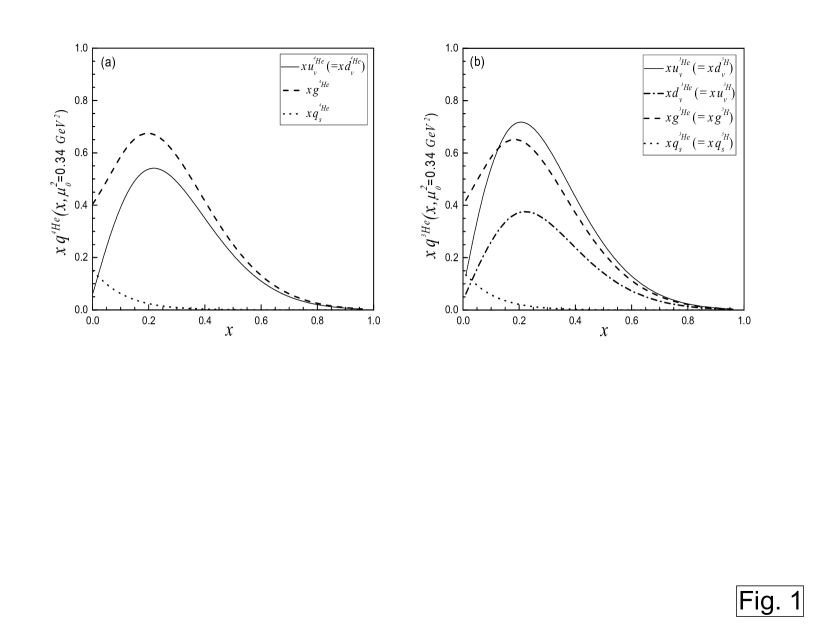
Figure 1: Panel (a): PDFs of ${}^{4}He$ nucleus versus $x$, for $(m_{a},\epsilon_{0}^{a})$ pair of (320, 120 $MeV$) ($a$ = ${\mathcal{U}}$, ${\mathcal{D}}$) and $b$ = 0.8 $fm$ at the hadronic scale, $\mu_{0}^{2}$ = 0.34 $GeV^{2}$. The dash curve represents the gluon distribution, while the solid and dotted curves indicate the valence and sea quark distributions, respectively. Panel (b): PDFs of ${}^{3}He$ nucleus versus $x$, for ($m_{\mathcal{U}}$, $\epsilon_{0}^{\mathcal{U}}$) and ($m_{\mathcal{D}}$, $\epsilon_{0}^{\mathcal{D}}$) pairs of (300, 130 MeV) and (325, 115 MeV), respectively, and $b$ = 0.8 $fm$ at the hadronic scale, $\mu_{0}^{2}$ = 0.34 $GeV^{2}$. The solid and dotted-dash curves are the valence up (down) and down (up) quark distributions of ${}^{3}He$ (${}^{3}H$) nucleus, respectively, while the dotted and dash curves indicate the sea quark and gluon distributions, respectively.

These resulted PDFs for the ${}^{4}He$ and ${}^{3}He$ nuclei, at the hadronic scale $\mu_{0}^{2}$ = 0.34 $GeV^{2}$, are shown in the panels (a) and (b) of figure 1, respectively.

Now, by using the standard DGLAP equations, the above PDFs which are obtained from the CQEM at the initial scale $\mu_{0}^{2}$, can be evolved to any higher energy scale $Q^{2}$ Botje . However, these conventional PDFs are not $k_{t}$-dependent distributions. So, to consider the transverse momentum explicitly, in the next section the KMR approach will be introduced to generate the double-scale UPDFs from these single-scale PDFs.

III The KMR formalism and the UPDF$s$ and SF calculations

It is well known that there are problems at small $x$ region m1 ; m2 ; m3 ; m4 . So one should use the general formalism such as CCFM which the transverse momentum of partons play the crucial role or the reggeon theory such as pameron model. However it was shown that the $k_{t}$-factorization formalism is capable to consider the precise kinematics of the process and an important part of the virtual loop corrections, via the survival probability factor $T$ (see below). On the other hand, if we work with integrated partons, we have to include the NLO (and sometimes the NNLO) contributions to account for these effects. These differences appear to cause a discrepancy between the integrated and unintegrated frameworks Kimber2 ; Kimber1 ; kimber3 .

A brief description of the KMR formalism as well as the SF formula in the $k_{t}$-factorization framework, is presented in the following subsections (A and B), respectively.

III.1 The KMR formalism

In this subsection, we briefly discuss about the KMR scheme to extract the UPDFs from the resulted integrated PDFs of the previous section, as inputs. The KMR formalism was first proposed by Kimber, Martin and Ryskin Kimber2 ; Kimber1 ; kimber3 . From the two scheme discussed in the reference Kimber2 we use the second approach which directly relates the UPDFs to the conventional PDFs. This formalism was also separately discussed in the reference kimber3 . Based on this scheme, the $LO$ DGLAP equations can be modified by separating the real and virtual contributions of the evolution, and the two-scale UPDFs, $f_{a}(x,k_{t}^{2},\mu^{2})$ ($a$ = $q$ or $g$), can be defined as follows:

$$f_{a}(x,k_{t}^{2},\mu^{2})=T_{a}(k_{t}^{2},\mu^{2})\sum\limits_{b=q,g}\Big{[}{\alpha_{s}(k_{t}^{2})\over{2\pi}}\int^{1-\Delta}_{x}dzP_{ab}^{(LO)}(z)b\Big{(}{x\over z},k_{t}^{2}\Big{)}\Big{]},$$ (26)

where $P_{ab}^{(LO)}$ represent the $LO$ splitting functions, which account for the probability of a parton of type $a$ with momentum fraction $x^{\prime\prime}$, $a(x^{\prime\prime},Q^{2})$, emerging from a parent parton of type $b$ with a larger momentum fraction $x^{\prime}$, $b(x^{\prime},Q^{2})$, through $z=x^{\prime\prime}/x^{\prime}$. The survival probability factor, i.e., Sudakov form factor $T_{a}$, which gives the probability that parton $a$ with transverse momentum $k_{t}$ remains untouched in the evolution up to the factorization scale $\mu$, is defined via the following equation:

$$T_{a}(k_{t}^{2},\mu^{2})=exp\Big{(}-\int^{\mu^{2}}_{k_{t}^{2}}{\alpha_{s}(k^{2})\over{2\pi}}{dk^{2}\over k^{2}}\sum\limits_{b=q,g}\int^{1-\Delta}_{0}{dz^{\prime}}P_{ab}^{(LO)}(z^{\prime})\Big{)},$$ (27)

The infrared cut-off, $\Delta$ = $1-z_{max}$ = $k_{t}/(\mu+k_{t}$), is determined by imposing the AOC on the last step of the evolution, and protects the $1/(1-z)$ singularity in the splitting functions arising from the soft gluon emission. In the KMR formulation, the key idea is that the dependence on the second scale $\mu$ of the UPDFs appears only at the last step of the evolution. By completing the procedures of producing the UPDFs from the KMR scheme, the UPDFs of the ${}^{4}He$, ${}^{3}He$ and ${}^{3}H$ nuclei can be evaluated by using their conventional PDFs (which were determined in the previous section), as inputs.

III.2 The SF in the $k_{t}$-factorization framework

Here it is briefly described the different steps to calculate the SF ($F_{2}(x,Q^{2})$) in the $k_{t}$-factorization framework, by using the KMR UPDFs as inputs. We explicitly investigate the separate contributions of gluons and (direct) quarks to the SF expression Kimber2 ; Kimber1 ; kimber3 .

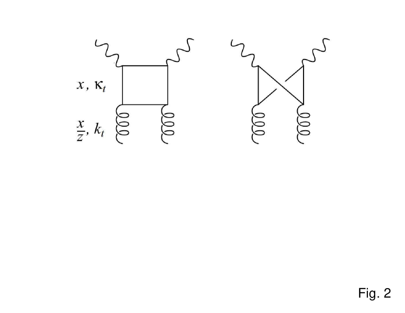
Figure 2: The quark box and crossed-box diagrams which demonstrate the contribution of the unintegrated gluon distributions, $f_{g}$($x$/$z$, $k_{t}^{2}$, $\mu^{2}$), to the structure function, $F_{2}$.

The unintegrated gluons can contribute to $F_{2}$ via an intermediate quark. As shown in the figure 2, both the quark box and crossed-box diagrams must be regarded as the gluon portions. The variable $z$ denotes the fraction of the gluon’s momentum that is transferred to the exchanged struck quark. The parameters $k_{t}$ and $\kappa_{t}$ indicate the transverse momentum of the parent gluons and daughter quarks, respectively. In the $k_{t}$-factorization framework, the unintegrated gluon contributions to $F_{2}$ can be obtained via the following equation Kimber1 ; Kimber2 ; kimber3 ; Kwiecinski ; Askew ; Stasto :

$$F_{2}^{g\rightarrow q\bar{q}}(x ,Q^{2})=\sum_{q}\>e_{q}^{2}{Q^{2}\over 4\pi}\int{dk_{t}^{2}\over{k_{t}^{4}}}\int_{0}^{1}d\beta\int d^{2}\kappa_{t}\>\alpha_{s}(\mu^{2})\>f_{g}\Big{(}{x\over z},k_{t}^{2},\mu^{2}\Big{)}\Theta\Big{(}1-{x\over z}\Big{)}$$

$$\times\Big{\{}[\beta^{2}+{(1-\beta)}^{2}]\>\Big{(}{\bm{\kappa}_{t}\over D_{1}}-{{\bm{\kappa}_{t}-\bm{k}_{t}}\over D_{2}}\Big{)}^{2}\>+\>[m_{q}^{2}+4Q^{2}\beta^{2}(1-\beta)^{2}]\Big{(}{1\over D_{1}}-{1\over D_{2}}\Big{)}^{2}\Big{\}}.$$ (28)

The variable $\beta$ is defined as the light-cone fraction of the photon’s momentum carried by the internal quark line. In addition, the denominator factors are defined as follows:

$$D_{1}=\kappa_{t}^{2}+\beta(1-\beta)Q^{2}+m_{q}^{2}$$

$$D_{2}=(\bm{\kappa}_{t}-\bm{k}_{t})^{2}+\beta(1-\beta)Q^{2}+m_{q}^{2}.$$ (29)

In the equation (III.2), the summation goes over various quark flavors $q$ with different masses $m_{q}$ which can appear in the box. In the present study, we consider three lightest flavor of quarks ($n_{f}$ = 3), i.e., $u$, $d$ and $s$, whose masses are neglected with a good approximation. So, $n_{f}$ = 3 throughout of our calculations. Additionally, the variable $z$ is defined as follows:

$${1\over z}=1\>+\>{{\kappa_{t}^{2}+m_{q}^{2}}\over{(1-\beta)Q^{2}}}\>+\>{{k_{t}^{2}+\kappa_{t}^{2}-2\>\bm{\kappa}_{t}\>.\>\bm{k}_{t}+m_{q}^{2}}\over{\beta Q^{2}}}.$$ (30)

which is the ratio of the Bjorken variable $x$ and the fraction of the proton momentum carried by the gluon. As in the reference Kwiecinski , the scale $\mu$, which controls the unintegrated gluon distribution and the QCD coupling constant $\alpha_{s}$, is chosen as follows:

$$\mu^{2}=k_{t}^{2}+\kappa_{t}^{2}+m_{q}^{2}.$$ (31)

The equation (III.2) gives the contributions of unintegrated gluons to $F_{2}$ in the perturbative region, $k_{t}$ $>$ $k_{0}$, where the UPDFs are defined. The smallest cutoff, $k_{0}$, we can choose, is the initial scale of order 1 $GeV$, at which the $k_{t}$-factorization scheme is defined Askew . For the contribution from the nonpertubative region, $k_{t}$ $<$ $k_{0}$, it can be approximated

$$\int_{0}^{k_{0}^{2}}{dk_{t}^{2}\over k_{t}^{2}}\>f_{g}(x,k_{t}^{2},\mu^{2})\>\Big{[}{\textit{remainder\>\>of\>\>equation}\>\>(\ref{25})\over k_{t}^{2}}\Big{]}\simeq\>xg(x,k_{0}^{2})\>T_{g}(k_{0},\mu)\>\Big{[}\quad\Big{]}_{k_{t}=a},$$ (32)

where $a$ is belong to the interval (0, $k_{0}$). The dependence on the choice of $a$ is numerically unimportant to the nonperturbative contribution Kimber1 ; Kimber2 ; kimber3 .

Now, the contributions of unintegrated quarks must be added to $F_{2}$. If an initial quark with Bjorken scale $x$/$z$ and perturbative transverse momentum $k_{t}$ $>$ $k_{0}$, splits to a radiated gluon and a quark with smaller Bjorken scale $x$ and transverse momentum $\kappa_{t}$, this final quark can then couple to the photon and contributes to $F_{2}$, as follows:

$$F_{2}^{q(perturbative)}(x,Q^{2})=\sum_{q=u,d,s}\>e_{q}^{2}\>\int_{k_{0}^{2}}^{Q^{2}}\> {d\kappa_{t}^{2}\over\kappa_{t}^{2}}\>{\alpha_{s}(\kappa_{t}^{2})\over{2\pi}}\int_{k_{0}^{2}}^{\kappa_{t}^{2}}\>{dk_{t}^{2}\over k_{t}^{2}}\int_{x}^{Q/{(Q+k_{t})}}\>dz$$

$$\times\Big{[}f_{q}\Big{(}{x\over z},k_{t}^{2},Q^{2}\Big{)}\>+\>f_{\bar{q}}\>\Big{(}{x\over z},k_{t}^{2},Q^{2}\Big{)}\Big{]}P_{qq}(z),$$ (33)

where during the quark evolution, AOC is imposed on the upper limit of the $z$ integration. Again, one must consider the nonperturbative contributions for the $k_{t}$ $<$ $k_{0}$,

$$F_{2}^{q(nonperturbative)}(x,Q^{2})=\sum_{q}e_{q}^{2}\>\Big{(}xq(x,k_{0}^{2})\>+\>x\bar{q}(x,k_{0}^{2})\Big{)}\>T_{q}(k_{0},Q),$$ (34)

which physically can be assumed as a quark or anti-quark, which does not experience real splitting in the perturbative region, and interacts unchanged, with the photon at the scale $Q$. So, a Sudakov-like factor, $T_{q}(k_{0},Q)$, is written to indicate the probability of evolution from $k_{0}$ to $Q$ without radiation.

Finally, by summing both gluon and quark contributions, one can obtain the overall SF in the $k_{t}$-factorization framework. Subsequently, the EMC ratio, which is defined as the ratio of the SF of the bound nucleon to that of the free nucleon, can be evaluated as follows Jaffe1 :

$$\mathcal{R}_{EMC}={F_{2}^{T}(x)\over{F^{T^{\star}}_{2}(x)}},$$ (35)

where $T$ stands for the target, averaged over nuclear spin and iso-spin and $T^{\star}$ is a hypothetical target with exactly the same quantum numbers but with no parton exchange Jaffe1 . So, if the overlap integral $\mathcal{I}$ is omitted in the momentum distribution formula, i.e., the equations (1)-(3), we can compute the SF of free nucleons. The effects of nuclear Fermi motion are neglected from both $T$ and $T^{\star}$. We utilize the KMR UPDFs to calculate the SFs, and the EMC ratios of ${}^{4}He$, ${}^{3}He$ and ${}^{3}H$ nuclei in the $k_{t}$ factorization approach, which will be presented in the next section.

IV Results, discussions, and conclusions

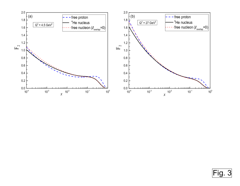
Figure 3: The comparison of the SFs of the ${}^{4}He$ nucleus in the KMR approach (the full curves) with those of the free proton using the MSTW-2008 data sets as inputs (the dash curves), at the energy scales 4.5 $GeV^{2}$ (panel (a)), and 27 $GeV^{2}$ (panel (b)). the dotted curves indicate our hypothetical free nucleon (by setting the overlap integral $\mathcal{I}$ equal to zero in the momentum density formula of ${}^{4}He$ nucleus) SFs in the KMR approach. All SFs are calculated with considering the three lightest quark flavors ($u$, $d$, $s$).

The overall SF, $F_{2}$, of ${}^{4}He$ nucleus in the $k_{t}$-factorization framework, using the KMR UPDFs, at the energy scales $Q^{2}$ = 4.5 and 27 $GeV^{2}$ are plotted in the panels (a) and (b) of Figure 3, respectively (the full curves). As expected, by increasing the scale $Q^{2}$ from 4.5 to 27 $GeV^{2}$, a considerable rise in $F_{2}$ at the smaller values of $x$ occurs. The dash curves in each panel, are the SFs of the free proton in the $k_{t}$-factorization framework, in which to generate the KMR UPDFs, the MSTW 2008 PDF sets are used as inputs. The SF of a hypothetical ${}^{4}He$ target, without any quark exchange between its nucleons (by ignoring the overlap integral $\mathcal{I}$ in the momentum density equation), i.e., the hypothetical free nucleon, in the $k_{t}$-factorization framework using the KMR UPDFs, are also exhibited in this figure for comparison (the dotted curves). The three lightest flavors of quarks, i.e., $u$, $d$ and $s$, are considered in calculation of these SFs. According to the equation (35), the EMC ratio in the $k_{t}$-factorization formalism at each energy scale, can be evaluated by regarding the ratio of the full curve (${}^{4}He$ SF) to the dotted curve (the hypothetical free nucleon SF). It is observed that the SFs of our hypothetical free nucleon are in overall good agreement with the SF of the free proton. Especially at the small $x$ region, as one should expect, the SFs of free nucleon (the dotted curves) and free proton (the dash curves) are approximately equal, since in this area, $u$ = $d$ = $\bar{u}$ = $\bar{d}$ and the proton and neutron SFs must be the same. The similar conclusions have been made for the ${}^{6}Li$ nucleus in our recent work, i.e., the reference Hadian4 .

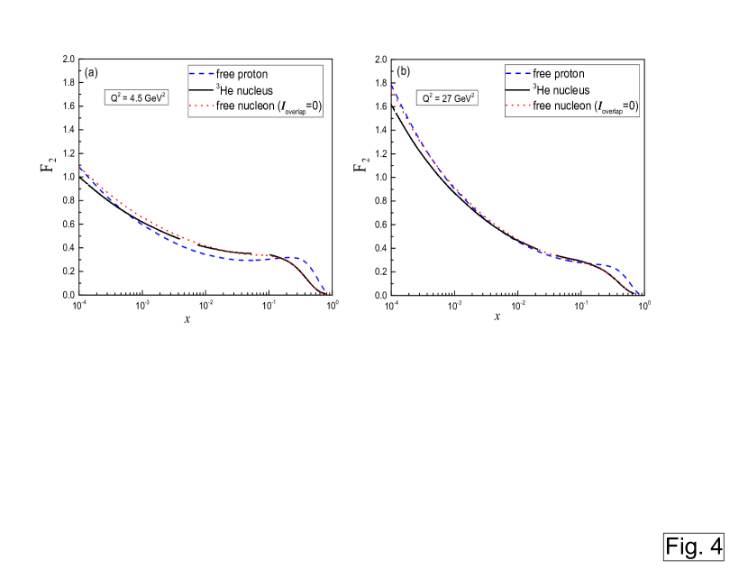
Figure 4: The same as the figure 3, but for the ${}^{3}He$ nucleus.

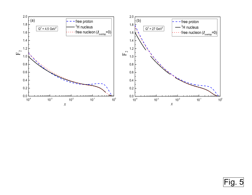
Figure 5: The same as the figure 3, but for the ${}^{3}H$ nucleus.

Figures 4 and 5 are the same as figure 3, but for the ${}^{3}He$ and ${}^{3}H$ nuclei, respectively. Similar to the figure 3, the SFs of free nucleon (the dotted curves) and free proton (the dash curves) are again approximately equal at the small $x$. Also, to obtain the EMC ratio in the $k_{t}$-factorization framework for these nuclei, one should again consider the ratio of the full curves to the dotted curves in each panel. In addition, as we increase the $Q^{2}$ value to 27 $GeV^{2}$, again, the overall SFs become greater.

The resulting EMC ratios of ${}^{4}He$, ${}^{3}He$ and ${}^{3}H$ nuclei in the $k_{t}$-factorization framework, using the KMR UPDFs, are plotted in the figures 6, 7 and 8, respectively. For each of these nuclei, the ratio is calculated at the energy scales $Q^{2}$ = 4.5 and 27 $GeV^{2}$. Due to neglecting the Fermi motion, the EMC ratios monotonically decrease and the growth in the EMC ratios at the large $x$ values do not occur. Therefore, the EMC ratios are illustrated for the $x\leq 0.7$ region. In the figure 6, the experimental measurements are from the JLab Seely ; Malace (filled circles), NMC New ; Malace (filled triangles), and SLAC Gomez ; Malace (filled squares), while in the figures 7 and 8, the filled circles and the filled squares are the experimental data from JLab Seely ; Malace and HERMES Malace ; Airapetisn , respectively. To compare the theoretical and experimental ${}^{4}He$ EMC ratios more clearly at the small $x$, the experimental NMC data are illustrated in the distinct diagrams with logarithmic scale, i.e., panels (b) and (d) of the figure 6. The dash curves in the panels (a) and (b) of the figure 6, are given from our prior work Hadian3 , in which the $k_{t}$ dependence of parton distribution functions were neglected in the ${}^{4}He$ EMC calculations. Obviously, at the small $x$ region, the present ${}^{4}He$ EMC results are extremely improved with respect to our previous outcomes Hadian3 . However, when the Bjorken scale $x$ is increased, the differences between the full and dash curves decrease, which show that the $k_{t}$-factorization scheme has an important effect on the EMC calculations at the small $x$ values Hadian4 ; Frankfurt1 ; Frankfurt2 , i.e., shadowing region. Therefore, the inclusion of $k_{t}$-dependent PDFs in the EMC calculation, can reproduce the general form of shadowing effect Hadian4 ; Frankfurt1 ; Frankfurt2 . The similar behavior is seen in the EMC curves of ${}^{3}He$ and ${}^{3}H$ nuclei (see the figures 7 and 8, respectively) as well as the EMC ratio of ${}^{6}Li$ nucleus (see the figure 10 of reference Hadian4 ). In addition, for all three nuclei which discussed here, the EMC curves at the energy scales 4.5 and 27 $GeV^{2}$ have approximately the same behavior (see also the EMC ratio of ${}^{6}Li$ nucleus in the figure 10 of reference Hadian4 ). This similarity is expected, because the EMC ratio are not $Q^{2}$ dependent, significantly (e.g. see the reference Gomez ).

The comparisons of EMC ratios of ${}^{6}Li$ (the dash-dotted curves), ${}^{4}He$ (the dash curves), ${}^{3}He$ (the dotted curves) and ${}^{3}H$ (the full curves) nuclei in the KMR approach at the energy scales 4.5 and 27 $GeV^{2}$ are displayed in the left and right panels of figure 9, respectively. The ${}^{6}Li$ EMC ratios are plotted from the reference Hadian4 . As expected, the EMC curves of ${}^{3}He$ and ${}^{3}H$ mirror nuclei are very close together, because of iso-spin symmetry assumption. However, by increasing the number of nucleons in the nucleus, the probabilities of quark exchanges among the nucleons are increased, which make the $\mathcal{R}_{EMC}$ to have greater deviation from unity.

In conclusion, the CQEM and the KMR UPDFs were used to obtain the EMC ratios of ${}^{4}He$, ${}^{3}He$ and ${}^{3}H$ nuclei in the $k_{t}$-factorization framework. To calculate the double-scale UPDFs, we needed the conventional single-scale PDFs for each nucleon as inputs. Therefore, the CQEM was employed to elicit the PDFs of these nuclei at the hadronic scale 0.34 $GeV^{2}$. Then, the resulted PDFs were evolved by the DGLAP evolution equations to the higher energy scales. Subsequently, by using the KMR UPDFs, the SFs of these nuclei in the $k_{t}$-factorization scheme were calculated at the energy scales $Q^{2}$ = 4.5 $GeV^{2}$ and 27 $GeV^{2}$. Subsequently, we compared the resulted SFs with the corresponding SF of free proton. Eventually, after computing the EMC ratios of ${}^{4}He$, ${}^{3}He$ and ${}^{3}H$ nuclei, they were compared with the experimental data. It was seen that the outcome EMC ratios astonishingly were consistent with the various experimental data. Especially, the $k_{t}$-factorization approach extremely improved the EMC ratios of mentioned nuclei at the shadowing region. Therefore, similar to our previous work Hadian4 , the reduction of EMC effect at the small $x$ region, which traditionally is known as the ”shadowing phenomena” Frankfurt1 ; Frankfurt2 , can be successfully explained in the $k_{t}$-factorization framework by using the KMR UPDFs.

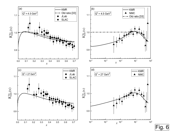
Figure 6: The EMC ratio of ${}^{4}He$ nucleus in the $k_{t}$-factoization framework by using the KMR UPDFs as inputs (the full curves), at the energy scales 4.5 $GeV^{2}$ (panels (a) and (b)), and 27 $GeV^{2}$ (panels (c) and (d)). The circles, the triangles, and the squares are from JLab Seely ; Malace , NMC New ; Malace , and SLAC Gomez ; Malace experimental data, respectively. the dotted-dash curves in the panels (a) and (b), are given from reference Hadian3 at $b$ = 0.8 $fm$ and $Q^{2}$ = 0.34 $GeV^{2}$, in which the contributions of UPDFs are not accounted in the ${}^{4}He$ EMC calculations.

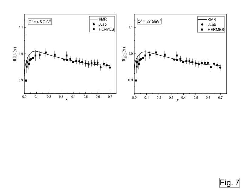
Figure 7: The EMC ratio of ${}^{3}He$ nucleus in the $k_{t}$-factoization framework by using the KMR UPDFs as inputs (the full curves), at the energy scales 4.5 $GeV^{2}$ (left panel), and 27 $GeV^{2}$ (right panel). The filled circles and the filled squares are the experimental data from JLab Seely ; Malace and HERMES Malace ; Airapetisn , respectively.

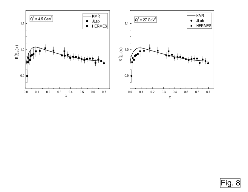
Figure 8: The same as the figure 7, but for the ${}^{3}H$ nucleus.

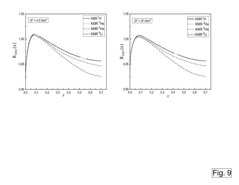
Figure 9: The comparisons of EMC ratios of ${}^{6}Li$ (the dash-dotted curves), ${}^{4}He$ (the dash curves), ${}^{3}He$ (the dotted curves) and ${}^{3}H$ (the full curves) nuclei in the KMR approach at the energy scales 4.5 $GeV^{2}$ (left panel) and 27 $GeV^{2}$ (right panel). The ${}^{6}Li$ EMC ratios are given from the reference Hadian4 .

References

- (1) V. N. Gribov and L. N. Lipatov, Yad. Fiz. 15 (1972) 781.
- (2) L. N. Lipatov, Sov. J. Nucl. Phys. 20 (1975) 94.
- (3) G. Altarelli and G. Parisi, Nucl. Phys. B 126 (1977) 298.
- (4) Y. L. Dokshitzer, Sov. Phys. JETP 46 (1977) 641.
- (5) E.G. de Oliveira, A.D. Martin, F.S. Navarra, M.G. Ryskin, J. High Energy Phys. 09 (2013) 158.
- (6) J.J. Aubert, et al., Phys. Lett. B 105 (1983) 403.
- (7) M. Modarres, A. Hadian, Phys. Rev. D 98 (2018) 076001.
- (8) L. L. Frankfurt and M. I. Strikman, Phys. Rep., 160 (1988) 235.
- (9) L. L. Frankfurt, V. Guzey,and M. I. Strikman, Phys. Rep., 512 (2012) 255.
- (10) M. Ciafaloni, Nucl. Phys. B 296 (1988) 49.
- (11) S. Catani, F. Fiorani, and G. Marchesini, Phys. Lett. B 234 (1990) 339.
- (12) S. Catani, F. Fiorani, and G. Marchesini, Nucl. Phys. B 336 (1990) 18.
- (13) G. Marchesini, Proceedings of the Workshop QCD at 200 TeV, Erice, Italy, edited by L. Cifarelli and Yu. L. Dokshitzer (Plenum, New York, 1992), p. 183.
- (14) G. Marchesini, Nucl. Phys. B 445 (1995) 49.
- (15) G. Marchesini, B. Webber, Nucl. Phys. B 349 (1991) 617.
- (16) G. Marchesini, B. Webber, Nucl. Phys. B 386 (1992) 215.
- (17) H. Jung, Nucl. Phys. B 79 (1999) 429.
- (18) H. Jung, G.P. Salam, Eur. Phys. J. C 19 (2001) 351.
- (19) H. Jung, J. Phys. G: Nucl. Part. Phys. 28 (2002) 971.
- (20) M. A. Kimber, Ph.D. thesis, University of Durham, 2001.
- (21) M. A. Kimber, A. D. Martin, and M. G. Ryskin, Phys. Rev. D 63, (2001) 114027.
- (22) M.A. Kimber , A.D. Martin, and M.G. Ryskin, Eur. Phys. J. C 12 (2000) 655.
- (23) M. Modarres and H. Hosseinkhani, Nucl. Phys. A 815, (2009) 40.
- (24) M. Modarres and H. Hosseinkhani, Few-Body Syst. 47, (2010) 237.
- (25) H. Hosseinkhani and M. Modarres, Phys. Lett. B 694, (2011) 355.
- (26) H. Hosseinkhani and M. Modarres, Phys. Lett. B 708, (2012) 75.
- (27) M. Modarres, H. Hosseinkhani, and N. Olanj, Nucl. Phys. A 902, (2013) 21.
- (28) M. Modarres, H. Hosseinkhani, N. Olanj, and M. R. Masouminia, Eur. Phys. J. C 75, (2015) 556.
- (29) M. Modarres, et al., Phys. Rev. D 94, (2016) 074035.
- (30) M. Modarres, et al., Nucl. Phys. B 926 (2018) 406.
- (31) M. Modarres, et al., Phys. Lett. B 772 (2017) 534.
- (32) M. Modarres, et al., Nucl. Phys. B 922 (2017) 94.
- (33) M. Modarres, H. Hosseinkhani, and N. Olanj, Phys. Rev. D 89, (2014) 034015.
- (34) M. Modarres, M. R. Masouminia, H. Hosseinkhani, and N. Olanj, Nucl. Phys. A 945, (2016) 168.
- (35) M. Modarres, A. Hadian, Eur. Phys. J. A (2018) to be published.
- (36) M. Modarres, M. Rasti, M. M. Yazdanpanah, Few-Body Syst. 55 (2014) 85.
- (37) M. Modarres, F. Zolfagharpour, Nucl. Phys. A 765 (2006) 112.
- (38) M. Botje, Comput. Phys. Commun. 182 (2011) 490, arXiv:1005.1481.
- (39) P. Hoodbhoy, R.L. Jaffe, Phys. Rev. D 35 (1987) 113.
- (40) P. Hoodbhoy, Nucl. Phys. A 465 (1987) 113.
- (41) R.P. Feynman, Photon Hadron Interactions, Benjamin, New York (1972).
- (42) F.E. Close, An Introduction to Quarks and Partons, Academic Press, London (1989).
- (43) R.G. Roberts, The Structure of the Proton, Cambridge University Press, New York (1993).
- (44) M. Modarres, A. Hadian, Nucl. Phys. A 966 (2017) 342.
- (45) M. Modarres, A. Hadian, Int. J. Mod. Phys. E 24 (2015) 1550037.
- (46) A. D. Martin, W. J. Stirling, R. S. Thorne, and G. Watt, Eur. Phys. J. C 63, (2009) 189.
- (47) A. D. Martin, W. J. Stirling, R. S. Thorne, and G. Watt, Eur. Phys. J. C 64, (2009) 653.
- (48) A. D. Martin, W. J. Stirling, R. S. Thorne, and G. Watt, Eur. Phys. J. C 70, (2010) 51.
- (49) G. Altarelli, N. Cabibbo, L. Maiani, R. Petronzio, Nucl. Phys. B 69 (1974) 531.
- (50) A. Manohar, H. Georgi, Nucl. Phys. B 234 (1984) 189.
- (51) S. Scopetta, V. Vento, M. Traini, Phys. Lett. B 421 (1998) 64.
- (52) M. Traini, V. Vento, A. Mair, A. Zambarda, Nucl. Phys. A 614 (1997) 472.
- (53) M. M. Yazdanpanah, M. Modarres, M. Rasti, Few-Body Syst. 48 (2010) 19.
- (54) S. Catani and F. Hautmann, Nucl.Phys.B, 427 (1994) 475.
- (55) A. Donnachie, H.G. Dosch, P.V. Landshoff and O. Nachtman, Pomeron physics and QCD, Cambridge University press, Cambridge (2002).
- (56) A. Donnachie and P.V. Landshoff, Eur.Phys.J., 77 (2017) 524.
- (57) Andersson et al, Eur.Phys.J.C, 25 (2002) 77.
- (58) J. Kwiecinski, A. D. Martin, and A. M. Stasto, Phys. Rev. D, 56 (1997) 3991.
- (59) A. J. Askew, J. Kwiecinski, A. D. Martin, and P. J. Sutton, Phys. Rev. D 47, (1993) 3775.
- (60) J. Kwiecinski, A. D. Martin, and A. M. Stasto, Acta Phys. Pol. B 28, (1997) 2577.
- (61) J. Seely, A. Daniel, D. Gaskell, J. Arrington et al., Phys. Rev. Lett. 103 (2009) 202301.
- (62) S. Malace, D. Gaskell, D.W. Higinbotham, I.C. Cloet, Int. J. Mod. Phys. E 23 (2014) 1430013.
- (63) New Muon Collaboration Collaboration (P. Amaudruz et al.), Nucl. Phys. B 441 (1995) 3.
- (64) J. Gomez, R. Arnold, P. E. Bosted, C. Chang et al., Phys. Rev. D 49 (1994) 4348.
- (65) A. Airapetisn et al., Phys. Lett. B 567 (2003) 339.